Changing Model Behavior at Test-Time Using Reinforcement Learning

1 Introduction

Machine learning models are often used at test-time subject to constraints and trade-offs not present at training-time. A computer vision model operating on an embedded device may need to perform real-time inference; a translation model operating on a cell phone may wish to bound its average compute time in order to be power-efficient. In these cases, there is often a tension between satisfying the constraint and achieving acceptable model performance. These constraints need not be restricted to speed and accuracy, but can reflect preferences for model simplicity or other desiderata.

One way to deal with constraints is to build them into models explicitly at training time. This has two major disadvantages: First, it requires manually designing and retraining a new model for each use case. Second, it doesn’t permit adjusting constraints at test-time in an input-dependent way.

In this work, we describe a method to change model behavior at test-time on a per-input basis. This method involves two components: The first is a model that we call a Composer. A Composer adaptively constructs computation graphs from sub-modules on a per-input basis using a controller trained with reinforcement learning to examine intermediate activations. The second is the notion of Policy Preferences, which allow test-time modifications of the controller policy.

This technique has several benefits: First, it allows for dynamically adjusting for constraints at inference time with a single trained model. Second, the Composer model can ‘smartly’ adjust for constraints in the way that is best for model performance (e.g. it can decide to use less computation on simpler inputs). Finally, it provides some interpretability, since we can see which examples used which resources at test-time.

The rest of this paper is structured as follows: In Section 2 we describe the Composer model, in Section 3 we describe Policy Preferences, and in Section 4 we present experimental results.

2 The Composer Model

The Composer Model (depicted in Figure 1) consists of a set of modules and a controller network. The modules are neural networks and are organized into ‘metalayers’. At each metalayer in the network, the controller selects which module will be applied to the activations from the previous metalayer (see also Eigen et al. (2013); Bengio et al. (2015); Andreas et al. (2016); Shazeer et al. (2017); Fernando et al. (2017); Denoyer & Gallinari (2014)).

Specifically, let the $i$th metalayer of the network be denoted $f_{i}$, with $f_{0}$ a special book-keeping layer, called the ‘stem’. For $i>0$, the $i$th metalayer is composed of $m_{i}$ functions, $f_{i,1},\ldots,f_{i,m_{i}}$ that represent the individual modules in the metalayer. Note that these modules can differ in terms of architecture, number of parameters, or other characteristics. There are $n$ metalayers, so the depth of the network is $n+1$ (including the stem). Once a selection of modules is made, it defines a neural network, which is trained with SGD.

The controller is composed of $n$ functions, $g_{1},\ldots g_{n}$ each of which output a policy distribution over the $m$ modules in the corresponding metalayer. In equations:

$$\vspace{-1cm}a_{0} =f_{0}(x)$$ (1)

$$p_{i} =g_{i}(a_{i-1},c_{i-1})$$ (2)

$$c_{i} \sim\text{Categorical}(p_{i})$$ (3)

$$a_{i} =f_{i,c_{i}}(a_{i-1})$$ (4)

$$p(y|x,c_{1:n}) =\text{softmax}(a_{n})\vspace{-1cm}$$ (5)

where $x$ is the input, $y$ is the ground truth labeling associated with $x$, $a_{i}$ are the network activations after the $i$th metalayer, $p_{i}$ are the parameters of the probability distribution output by the controller at step $i$, $c_{i}$ is the module choice made by sampling from the controller’s distribution at step $i$, $c_{1:n}$ denotes $c_{1},\ldots,c_{n}$, and $p_{1:n}$ similarly denotes $p_{1},\ldots,p_{n}$.

The controller can be implemented as an RNN by making the controller functions share weights and a hidden state. We train the controller to optimize the reward $\log p(y|x,c_{1:n})$ using REINFORCE (Williams, 1992). For details, see Appendix A.

Figure 1: A diagram of the Composer model. This Composer has 3 metalayers each consisting of 2 modules. Circles denote stochastic nodes; squares denote deterministic nodes.

3 Policy Preferences

We can augment the reward function of the controller to express preferences we have about its policy over computation graphs. Implemented naively, this does not allow for test-time modification of the preferences. Instead, we add a cost $C(p_{1:n},c_{1:n},\gamma)$ to the reward for the controller, where $\gamma$ is a preference value that can be changed on either a per-input or per-mini-batch basis.

Crucially, $\gamma$ is given as an input to the controller. At train-time, we sample $\gamma\sim\Gamma$, where $\Gamma$ is a distribution over preferences. Because of this, the controller learns at training time to modify its policy for different settings of $\gamma$. At test time, $\gamma$ can be changed to correspond to changing preferences. The specific dependence of $C$ on the action and the preference can vary: $\gamma$ need not be a single scalar value.

Below we describe two instances of Policy Preferences applied to the Composer model. Policy Preferences could also be applied in a more general reinforcement learning setting.

3.1 Glimpse Preferences

For a variety of reasons we might want to express test-time preferences about model resource consumption (see also Graves (2016); Figurnov et al. (2016)). One environment where this might be relevant is when the model is allowed to take glimpses of the input that vary both in costliness and usefulness. If taking larger glimpses requires using more parameters, we can achieve this by setting

$$C_{1}(p_{1:n},c_{1:n},\gamma)=-\gamma\sum_{i=1}^{n}\beta_{i,c_{i}}.$$ (6)

where $\beta_{i}\in\mathbb{R}^{m}$ is the vector of parameter counts for each module in the $i$th metalayer and $\beta_{i,c_{i}}$ is the parameter count for the module chosen at the $i$th metalayer. $C_{1}$ is applied per-element here.

3.2 Entropy Preferences

Because the modules and the controller are trained jointly, there is some risk that the controller will give all of its probability mass to the module that happens to have been trained the most so far. To counteract this tendency we can use another cost

$$C_{2}(p_{1:n},c_{1:n},\gamma)=-\gamma\sum_{i=1}^{n}\left|\left|\frac{1}{N}\sum_{j=1}^{N}p_{i}^{(j)}\right|\right|_{2}^{2}.$$ (7)

where $N$ is the number of examples in a batch and $p_{i}^{(j)}\in\mathbb{R}^{m}$ is the vector of module probabilities produced by the controller at metalayer $i$ for batch element $j$. Note that this reward is maximized when the controller utilizes all modules equally within a batch. $C_{2}$ is applied per-batch.

One could simply augment the controller reward with a similar bonus and anneal the bonus to zero during training, but our method has at least two advantages: First, if load balancing between specialized modules must be done at test time, using Policy Preferences allows it to be done in a ‘smart’ way. Second, this method removes the need to search for and follow an annealing schedule - one can stop training at any time and set the test-time batch-entropy-preference to 0.

4 Experimental Results

We test the claim that one can dynamically adjust the amount of computation at inference time with a single trained model using a Composer and Policy Preferences. We introduce a modified version of MNIST called Wide-MNIST to accomplish this: Images in Wide-MNIST have shape $28\times 56$, with a digit appearing in either the left half or the right half of the image. Each image is labeled with one of 20 classes (10 for ‘left’ digits and 10 for ‘right’ digits). We train a Composer model with two modules - a large module that glimpses the whole input and a small module that glimpses only the left side. The Composer is trained using both entropy preferences and glimpse preferences. See Figure 2 for results, which support the above claim. See Appendix B for qualitative experiments.

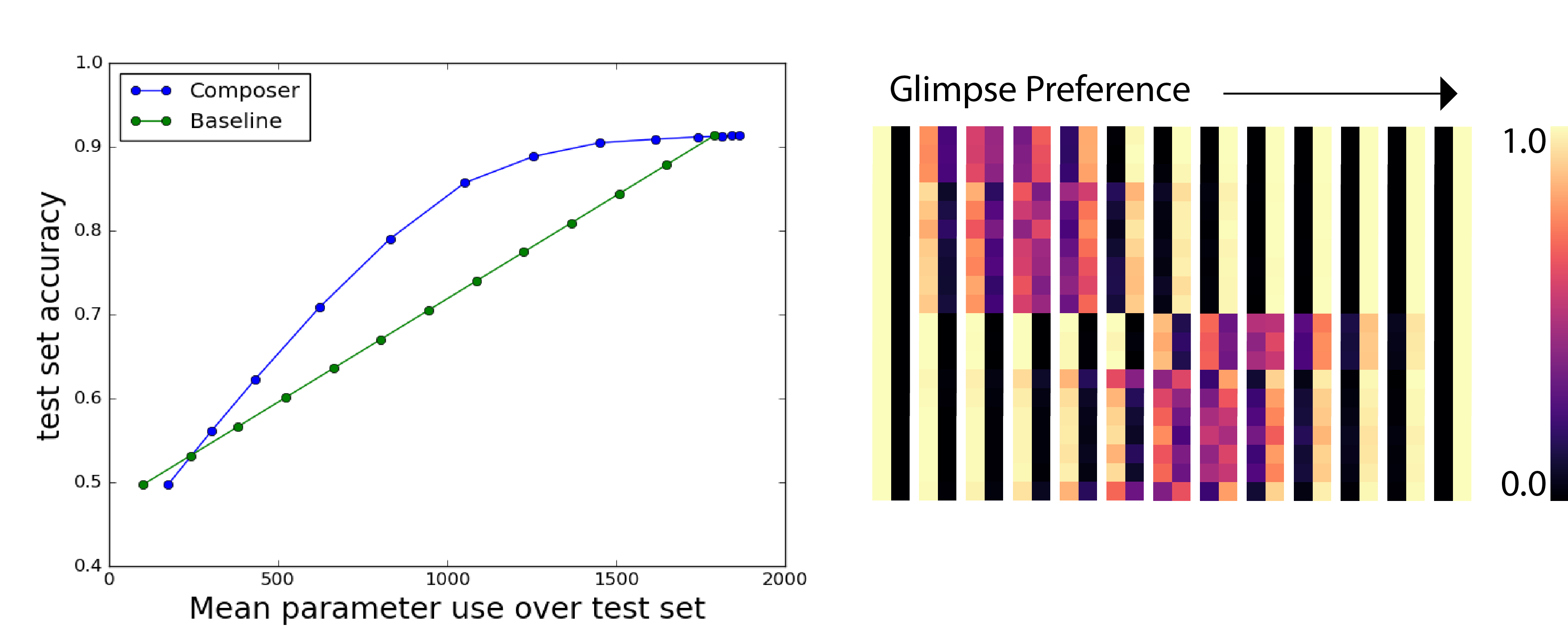
Figure 2: Changing the glimpse preference at test time for a model trained on the Wide-MNIST data-set. Note that all data points on the curve labeled ‘Composer’ come from a single trained model. (Left): The Composer model consists of a small module that only glimpses the left side of the input and a large model that glimpses the whole input, but uses more parameters to do so. It is evaluated at a variety of glimpse preference values, resulting in a variety of average-parameter-use values. A baseline model is created by randomly choosing between the large module and the small module some varying fraction of the time, in order to induce different average-parameter-use values. The gap between the Composer curve and the baseline curve represents the extent to which the controller has ‘smartly’ adapted its module use based on the input example. (Right): Heat-maps denote probabilities assigned by the controller to each module, for each of the 20 labels, averaged over the whole test set. The left column corresponds to the small module and the right column to the large module. The top 10 rows correspond to ‘right’ digits and the bottom 10 rows correspond to ‘left’ digits. As the glimpse preference is decreased, the controller first chooses to use the small module for ‘left’ digits, since this doesn’t cause much loss in classification accuracy. Only when the glimpse preference gets very low does the controller assign ‘right’ digits to the small module.

5 Acknowledgements

We thank Kevin Swersky, Hugo Larochelle, and Sam Schoenholz for helpful discussions.

Appendix A Policy Gradient Details

For simplicity let $c=c_{1:n}$ and $p=p_{1:n}$. Then, we use REINFORCE/policy gradients to optimize the objective

$$\textbf{E}_{c}\left[\log p(y|x,c)\right]$$ (8)

Jensen’s inequality tells us that this is a lower bound on what we truly seek to optimize, $\log p(y|x)$

$$\log p(y|x)=\log\textbf{E}_{c}\left[p(y|x,c)\right]\geq\textbf{E}_{c}\left[\log p(y|x,c)\right].$$

To maximize this expectation we perform gradient ascent. The gradient of this quantity with respect to the model parameters $\theta$ is

$$\textbf{E}_{c}\left[\nabla_{\theta}\log p(y|x,c)+\log p(y|x,c)\nabla_{\theta}\log p(c|x)\right].$$ (9)

To implement the policy preference cost functions we can modify our reward to include $C(p,c,\gamma)$. In this case our objective becomes

$$\textbf{E}_{c}\left[\log p(y|x,c)+C(p,c,\gamma)\right]$$ (10)

and the gradient becomes

$$\textbf{E}_{c}\left[\nabla_{\theta}(\log p(y|x,c)+C(p,c,\gamma))+(\log p(y|x,c)+C(p,c,\gamma))\nabla_{\theta}\log p(c|x)\right].$$ (11)

Appendix B Qualitative Experiments

This section contains various qualitative explorations of Composer models trained with and without Policy Preferences.

B.1 Module Specialization

On MNIST, modules often specialize to digit values of of 8, 5, and 3 or 4, 7, and 9, which are the most frequently confused groups of digits. See Figure 3 for an example of this behavior.

Figure 3: Modules choices in the first metalayer of a random minibatch for a Composer with 3 modules at each metalayer. The number of parameters in each module increases from top to bottom, with the second module having twice as many parameters as the first, and the third module having three times as many. This Composer was trained using a Policy Preference penalizing the parameter count of the chosen module. Each row corresponds to a module, and the module size increases from top to bottom. The bottom module seems to act as a 4,7,9 disambiguator.

Tests on CIFAR-10 yielded similar results: See Figure 4.

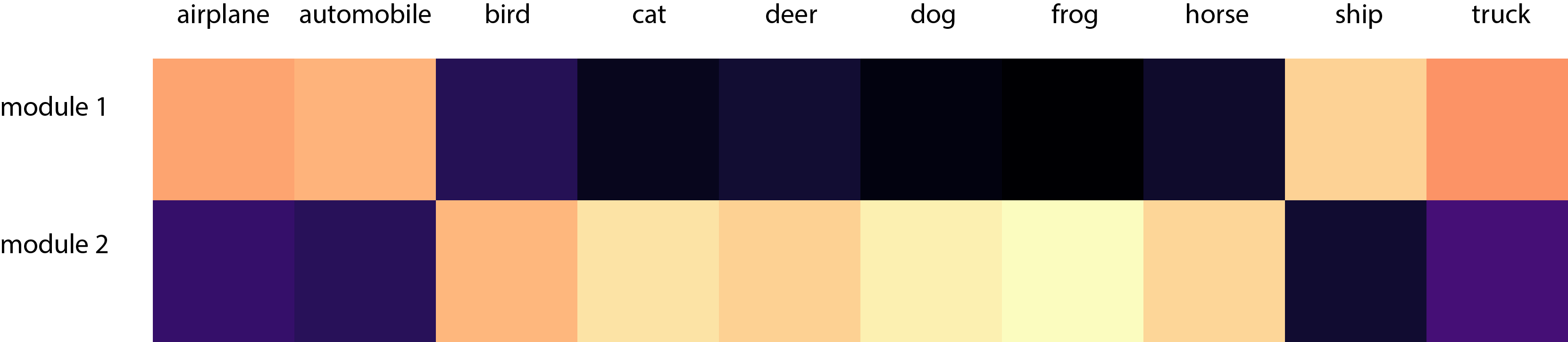
Figure 4: A heatmap demonstrating the probability the controller assigned to using each module in the first metalayer, for each class in CIFAR-10. Note that the controller has divided up the data into essentially two groups - man-made things and natural things.

B.2 Entropy Preferences

We also conducted an ablation experiment demonstrating that the batch entropy preference results in better module utilization. See Figure 5 for results. In addition, we show the result of modifying the test-time entropy preference of a model that has been trained with a standard entropy penalty (Figure 6). This could be useful in a variety of contexts (e.g. language modeling).

Figure 5: The effect of the batch entropy preference on module selection frequency for a Composer with 1 metalayer and 4 modules trained on MNIST. These are module selection heatmaps similar to those in the above figures. (Left) With the entropy preference, modules are utilized more equally. After 100k steps, the mutual information between module choices and class labels for this run is 0.9 nats. (Right) With a normal entropy penalty, some modules ‘get ahead’ and others never catch up. After 100k steps, the mutual information for this run is only 0.43 nats. This test was conducted with a constant, zero-variance value for the preference, so in this case the non-batch entropy preference is equivalent to the standard entropy penalty (which involves a sum of separate entropy penalties - one per example).

Figure 6: Modifying the test-time entropy preference of a model trained using an ‘unbatched’ entropy penalty.

References

- Andreas et al. (2016) Jacob Andreas, Marcus Rohrbach, Trevor Darrell, and Dan Klein. Learning to compose neural networks for question answering. CoRR, abs/1601.01705, 2016. URL http://arxiv.org/abs/1601.01705.
- Bengio et al. (2015) Emmanuel Bengio, Pierre-Luc Bacon, Joelle Pineau, and Doina Precup. Conditional computation in neural networks for faster models. arXiv preprint arXiv:1511.06297, 2015.
- Denoyer & Gallinari (2014) Ludovic Denoyer and Patrick Gallinari. Deep sequential neural network. arXiv preprint arXiv:1410.0510, 2014.
- Eigen et al. (2013) David Eigen, Marc’Aurelio Ranzato, and Ilya Sutskever. Learning factored representations in a deep mixture of experts. arXiv preprint arXiv:1312.4314, 2013.
- Fernando et al. (2017) Chrisantha Fernando, Dylan Banarse, Charles Blundell, Yori Zwols, David Ha, Andrei A. Rusu, Alexander Pritzel, and Daan Wierstra. Pathnet: Evolution channels gradient descent in super neural networks. CoRR, abs/1701.08734, 2017. URL http://arxiv.org/abs/1701.08734.
- Figurnov et al. (2016) Michael Figurnov, Maxwell D. Collins, Yukun Zhu, Li Zhang, Jonathan Huang, Dmitry P. Vetrov, and Ruslan Salakhutdinov. Spatially adaptive computation time for residual networks. CoRR, abs/1612.02297, 2016. URL http://arxiv.org/abs/1612.02297.
- Graves (2016) Alex Graves. Adaptive computation time for recurrent neural networks. CoRR, abs/1603.08983, 2016. URL http://arxiv.org/abs/1603.08983.
- Shazeer et al. (2017) Noam Shazeer, Azalia Mirhoseini, Krzysztof Maziarz, Andy Davis, Quoc V. Le, Geoffrey E. Hinton, and Jeff Dean. Outrageously large neural networks: The sparsely-gated mixture-of-experts layer. CoRR, abs/1701.06538, 2017. URL http://arxiv.org/abs/1701.06538.
- Williams (1992) Ronald J Williams. Simple statistical gradient-following algorithms for connectionist reinforcement learning. Machine learning, 8(3-4):229–256, 1992.