Nikhef 2017-010

Electroweak stability and non-minimal coupling

Marieke Postma and Jorinde van de Vis

Nikhef,
Science Park 105,
1098 XG Amsterdam, The Netherlands

ABSTRACT

The measured values of the Higgs and top quark mass indicate that the electroweak vacuum is metastable if there is no new physics below the Planck scale. This is at odds with a period of high scale inflation. A non-minimal coupling between the Higgs field and the Ricci scalar can stabilize the vacuum as it generates a large effective Higgs mass during inflation. We consider the effect of this coupling during preheating, when Higgs modes can be produced very efficiently due to the oscillating Ricci scalar. We compute their effect on the effective potential and the energy density. The Higgs excitations are defined with respect to the adiabatic vacuum. We study the adiabaticity conditions and find that the dependence of our results on the choice of the order of the adiabatic vacuum increases with time. For large enough coupling particle production is so efficient that the Higgs decays to the true vacuum before this is an issue. However, for smaller values of the Higgs-curvature coupling no definite statements can be made as the vacuum dependence is large.

1 Introduction

No evidence for physics beyond the Standard Model (SM) has been found so far at the Large Hadron Collider or any other experiment. This opens up the possibility of the desert scenario, in which the SM is valid up to Planck scale energies. If true, our universe might be metastable. Indeed, with the particle content of the SM, the Higgs quartic coupling $\lambda$ runs to negative values at large energy scales, and the Higgs potential develops a second minimum in addition to the electroweak minimum. For the best fit values of the top quark and Higgs mass the quartic Higgs coupling becomes zero $\lambda(\mu_{\rm cr})=0$ at a scale $\mu_{\rm cr}\sim 10^{11}$ GeV, although stability of the SM up to the Planck scale is only excluded at the 2-3$\sigma$ level [1, 2, 3, 4, 5, 6, 7]. In this paper we will take the instability of the Higgs potential at face value, and consider its cosmological consequences.

The presence of the global minimum at large field values poses no danger at present as the metastable vacuum can only decay via a slow tunnelling process, and has a lifetime that is much longer than the age of the universe. Within a cosmological context the longevity of our vacuum is no longer assured. If the Hubble scale $H$ during inflation is comparable or larger than the maximum of the Higgs potential, then vacuum decay is no longer suppressed as the Higgs field can quantum fluctuate over the potential barrier [8, 9, 10, 11, 12]. This is a concern for large field inflationary models such as chaotic inflation and Starobinsky type inflation. It was pointed out that stability during inflation can be ensured if one includes a (positive) non-minimal coupling $\xi$ between the Ricci scalar and the Higgs field $\mathcal{L}\supset\frac{1}{2}m_{\rm P}^{2}R(1-2\xi\Phi^{\dagger}\Phi)$ [13, 14, 15], as this induces an effective stabilizing Higgs mass. The vacuum is stable during inflation if $\xi\gtrsim 3/8$, but even smaller couplings $\xi\gtrsim 0.01$ are admissible depending on post-inflationary evolution [14]. The non-minimal coupling to gravity is allowed by all symmetries, in fact such a term will be generated by loop effects, although it is not clear whether it will have the right sign and size.

This is not the end of the story though. After inflation, as the inflaton starts oscillating at the bottom of its potential, the effective Higgs mass induced by the non-minimal coupling oscillates between positive and negative values, which can give rise to efficient production of Higgs quanta in a non-perturbative process called preheating [16, 17, 18, 19, 20, 21, 22]. The produced Higgs quanta contribute to the effective Higgs mass and the energy momentum tensor — this is similar to temperature corrections in a thermal bath, although the Higgs spectrum is highly non-thermal — and both effects can affect vacuum stability [23]. Preheating is efficient if

$$q_{0}\equiv\frac{3}{4}\left(\xi-\frac{1}{6}\right)\frac{\chi_{0}^{2}}{m_{\rm P}^{2}}\gtrsim\mathcal{O}(5),$$ (1)

with $\chi_{0}$ the inflaton field value at the end of inflation. In this case particle production is explosive, and within a few inflaton oscillations the produced quanta will completely dominate the Higgs mass. As this all happens at high scales $H>\mu_{\rm cr}$ the quantum contribution to the effective mass is negative and destabilizes the vacuum [23, 24, 25, 26, 27].

For smaller $q_{0}$-values results are less clear, and there is no consensus in the literature on the fate of our vacuum, mainly because different criteria for stability are used [23, 24, 25, 26, 27]. Even though in this case particle production is not efficient enough initially to destabilize the vacuum, this may still happen eventually as the classical potential red shifts away faster than the quantum corrections due to Higgs production. If the Higgs mass is dominated by the production term only after the Hubble scale has dropped below the critical value $H<\mu_{\rm cr}$, the quantum contribution to the effective mass is positive around the maximum of the potential, and thus will only raise the barrier separating the true and false vacuum. Nevertheless, tunnelling to the true vacuum may be enhanced by the non-zero energy density. Although a full calculation is needed to assert this effect, we expect decay to be fast when the energy density becomes of the order of the maximum of the potential. For small $q_{0}$ we will use this as our criterion for stability.

Arguably the most interesting part of parameter space is $q_{0}\lesssim 1$. From a naturalness point of view order one couplings $\xi$ are favored, and for both chaotic and Starobinksy type inflation models $\chi_{0}\sim 1$, which implies $q_{0}=\mathcal{O}(1)$. One of the main points of this paper is that exactly for these $q_{0}$-values the effective Higgs mass and especially the energy density will depend sensitively on the choice of vacuum, and no definite statements about stability can be made.

The Higgs mass, which gets a one-loop correction proportional to the Higgs two-point Green function, as well as the energy density can be split in a divergent vacuum piece, which is absorbed in counterterms and leads to the running of the couplings, and a finite piece due to Higgs excitations on top of the vacuum. Different choices of vacuum can be viewed as different renormalization schemes, as they lead to different renormalization conditions defining the physical couplings. In a cosmological setting where the background energy density in the inflaton field is changing with time, the vacuum choice is not well-defined. Usually, the zeroth order adiabatic vacuum is chosen. In the asymptotic regions where the system is (nearly) time-independent — at initial times during slow roll inflation and at final times after inflaton decay — it reduces to the usual in/out vacua. Moreover, if the background is slowly changing with time the production of high momentum modes is exponentially suppressed, supporting the vacuum interpretation [28].

The high momentum modes are adiabatic during at least part of the inflaton oscillation, and these moments in time can be used to evaluate the Green function. The problem with the current set-up is that smaller momentum modes $k<k_{n}$ violate the $n$th order adiabaticity condition and are never adiabatic. Since $k_{n}$ increases with time, the contribution of these non-adiabatic modes to the Higgs mass and energy density increases with time until they fully dominate the result. A direct way to monitor the vacuum dependence is to compare quantities calculated using the zeroth and second order adiabatic vacuum.

Of course, the electroweak vacuum is either stable or unstable, this cannot depend on the choice of vacuum. However, the problem is in defining the renormalized couplings in the theory — which is necessary to find a critical coupling below which the vacuum is stable — as different vacuum choices correspond to different counterterms. As usual this freedom can be fixed by measuring the couplings. However, this measurement has to be done during preheating, since different adiabatic vacua only give different results during preheating and not in the adiabatic initial and final states. Moreover, even if such a measurement was in principle possible, one would also need to use non-adiabatic methods to calculate the Green function for the results to be useful.

This paper is organized as follows. In the next section we introduce the Lagrangian and derive the equations of motion for the inflaton and Higgs field. In section 3 we then discuss the one-loop corrections to the effective potential and energy density, which are defined via an adiabatic renormalization scheme. Semi-analytic approximations of the effective Higgs mass and energy density are given in section 4, as well as a comparison with the numerical results. In section 5 we study the adiabaticity conditions and compute the vacuum dependence of the quantities of interest. In section 6 we formulate our criteria for vacuum stability, discuss relevant time scales and corroborate our analytic results with numerical calculations. We end with concluding remarks.

Notation.

We use a metric that is mostly positive $(-,+,+,+)$, and we set the reduced Planck mass to unity $m_{\rm P}^{2}=(8\pi G_{N})^{-1}=1$.

The relevant equations depend on the combination $(\xi-1/6)$, for which we introduce the shorthand notation

$$\hat{\xi}\equiv\left(\xi-\frac{1}{6}\right).$$ (2)

Time is measured in number of inflaton oscillations $T$. The frequency of the Higgs perturbations is periodic with frequency $\delta T=\frac{1}{2}$. To indicate a particular time during an oscillation, we use the notation $T{\hat{=}}\frac{1}{4}$, meaning $T=\frac{1}{4}$ mod $\frac{1}{2}$.

The inflaton background is an oscillating function with a time-dependent amplitude $A(T)$. The initial conditions for the inflaton field amplitude and scale factor at $T=0$ are denoted by $A(0)=A_{0}$ and $a(0)=a_{0}$. We will also need the amplitude and scale factor at $T=1/4$, which are denoted by $A(\frac{1}{4})=A_{1/4}$ and $a(\frac{1}{4})=a_{1/4}$. Finally, after a few oscillations the amplitude and scale factor are well approximated by $A(T)=A_{T}/T$ and $a(T)=a_{T}T^{2/3}$, with normalization constants $A_{T}$ and $a_{T}$. The values for all of them are taken from the numerical solution of the classical background. For future reference we list them here

$$\{A_{0},\,a_{0}\}=\{1/2,\,1\},\quad\{A_{1/4},\,a_{1/4}\}\approx\{0.1,\,1.3\},\quad\{A_{T},\,a_{T}\}\approx\{0.25,\,1.7\}.$$ (3)

2 Classical action

We study a Higgs field that is non-minimally coupled to the Ricci scalar. We are interested in the behavior during preheating, the period just after the end of inflation when the inflaton is oscillating in its potential, and the inflaton field still dominates the energy density. The Lagrangian is given by

$$\frac{\mathcal{L}}{\sqrt{-g}}=\frac{1}{2}\left(1-2\xi\Phi^{\dagger}\Phi\right)R+\mathcal{L}_{\rm SM}+\mathcal{L}_{\rm inf},$$ (4)

with $\Phi$ the SM Higgs doublet.

2.1 Inflaton background

For the inflaton we take a quadratic potential

$$\frac{\mathcal{L}_{\rm inf}}{\sqrt{-g}}=-\frac{1}{2}(\partial\chi)^{2}-\frac{1}{2}m_{\chi}^{2}\chi^{2}.$$ (5)

This is a good approximation for many inflationary models soon after the end of inflation, as for small field values $\chi\ll 1$ the potential is generically dominated by the quadratic term. However, since most of the Higgs fluctuations are produced during the first few inflaton oscillations, where deviations from the quadratic potential can be significant, for example in Starobinksy inflation, more precise calculations may require a model dependent inflaton potential.

The inflaton dominates the energy density in the universe. The Hubble constant and Ricci scalar can then be expressed in terms of the inflaton field:

$$3H^{2}\simeq\frac{1}{2}\dot{\chi}^{2}+\frac{1}{2}m_{\chi}^{2}\chi^{2},\qquad R=6\left(\dot{H}+2H^{2}\right)\simeq-\dot{\chi}^{2}+2m_{\chi}^{2}\chi^{2}.$$ (6)

The equation of motion for the inflaton is:

$$\ddot{\chi}+3H\dot{\chi}+m_{\chi}^{2}\chi=0.$$ (7)

We choose initial conditions at time $t_{0}=2\pi/m_{\chi}$ for the inflaton field and scale factor

$$A_{0}\equiv\chi(t_{0})=\frac{1}{2},\quad\dot{\chi}(t_{0})=0,\quad a(t_{0})=1.$$ (8)

We take $m_{\chi}=10^{-5}$ for the inflaton mass, which is the right order of magnitude for both chaotic inflation with a quadratic potential and Starobinsky inflation; in both models $\chi\sim 1$ at the end of inflation, in agreement with (8).

After a few oscillations the inflaton background is very well approximated by a periodic cosine function with a decreasing amplitude

$$\chi\approx\frac{A_{T}\cos(2\pi T)}{T},$$ (9)

with amplitude $A_{T}\approx 0.25$, which is determined by a fit to the numerical solution. The number of inflaton oscillations $T$ is approximated by

$$T\approx\frac{m_{\chi}t}{(2\pi)}-1.$$ (10)

After the first few oscillations the inflaton starts to behave as a cold dark matter fluid, i.e., averaged over an oscillation the inflaton has zero pressure and the energy density red shifts as $\rho_{\chi}\propto a^{-3}$. The scale factor grows as $a\propto t^{2/3}$, which can be written as

$$a\simeq a_{T}T^{2/3},$$ (11)

with $a_{T}\approx 1.7$. At late times the Ricci scalar and Hubble constant evolve as

$$R=\frac{A_{T}^{2}m_{\chi}^{2}(1+3\cos(4\pi T))}{2T^{2}}+\mathcal{O}(T^{-3}),\qquad H^{2}=\frac{A_{T}^{2}m_{\chi}^{2}}{6T^{2}}+\mathcal{O}(T^{-3}).$$ (12)

2.2 Mode equation for the Higgs field

The relevant part of the Lagrangian for the production of Higgs modes is

$$\frac{\mathcal{L}}{\sqrt{-g}}=\frac{1}{2}\left(1-2\xi|\Phi|^{2}\right)R-|D_{\mu}\Phi|^{2}-V+...$$ (13)

with the Higgs potential

$$V=-\mu^{2}|\Phi|^{2}+\lambda|\Phi|^{4}.$$ (14)

During preheating the Higgs mass $\mu^{2}$ is very small compared to the effective mass generated by the coupling to $R$, and will be neglected in our computations. We concentrate on the production of the radial Higgs field, and neglect all other SM particles. In unitary gauge $\Phi^{\dagger}\Phi=\Phi_{R}^{2}/2$, with $\Phi_{R}$ a real scalar that can be split in a background field plus fluctuations:

$$\Phi_{R}(\vec{x},t)=\phi(t)+\varphi(\vec{x},t).$$ (15)

We are interested in the regime of small Higgs field values $\xi\phi^{2}\ll 1$, then to leading order the results are the same in the Einstein and Jordan frame. This allows to treat gravity as a classical background. The FRW metric for a homogeneous isotropic universe is

$${\rm d}s^{2}=-{\rm d}t^{2}+a^{2}(t){\rm d}\vec{x}^{2}=a^{2}(\tau)\left(-{\rm d}\tau^{2}+{\rm d}\vec{x}^{2}\right).$$ (16)

The conformal time $\tau$ is defined via ${\rm d}\tau={\rm d}t/a(t)$. Derivatives with respect to coordinate time $t$ are denoted by an overdot and derivatives with respect to conformal time by a prime.

Using conformal time and defining ‘conformal’ fields

$$\bar{\phi}=a\phi,\quad\bar{\varphi}=a\varphi,\quad\bar{V}=a^{4}V,$$ (17)

the action for the fluctuations becomes (where we neglected the quartic self-interaction term)

$$S \supset\frac{1}{2}\int{\rm d}^{3}x{\rm d}ta^{3}\left[\dot{\varphi}^{2}+\frac{(\nabla\varphi)^{2}}{a^{2}}-\xi R\varphi^{2}-V_{\phi\phi}\varphi^{2}\right]$$

$$=\frac{1}{2}\int{\rm d}^{3}x{\rm d}\tau\left[\left(\partial_{\tau}\bar{\varphi}\right)^{2}+(\nabla\bar{\varphi})^{2}-M^{2}\bar{\varphi}^{2}-2\frac{a^{\prime}}{a}\bar{\varphi}\partial_{\tau}\bar{\varphi}+\left(\frac{a^{\prime}}{a}\right)^{2}\bar{\varphi}^{2}-\frac{1}{6}a^{2}R\bar{\varphi}^{2}\right]$$

$$=\frac{1}{2}\int{\rm d}^{3}x{\rm d}\tau\left[\left(\partial_{\tau}\bar{\varphi}\right)^{2}+(\nabla\bar{\varphi})^{2}-M^{2}\bar{\varphi}^{2}\right],$$ (18)

with the background dependent, and thus time-dependent, effective mass term

$$M^{2}=a^{2}\left(\left(\xi-\frac{1}{6}\right)R(t)+V_{\phi\phi}\right).$$ (19)

In the second step we switched to conformal time and fields. To get the final expression we integrated by parts and further used that $(a^{\prime}/a)=aH$, $R=6(\dot{H}+2H^{2})$, and $\partial_{\tau}(a^{\prime}/a)=(aH)^{2}+a^{2}\dot{H}$. The system is now equivalent to that of a harmonic oscillator with a time dependent frequency in Minkowski space, and we can apply the usual flat space methods. The field $\bar{\varphi}$ can be expanded in mode functions

$$\bar{\varphi}=\int\frac{{\rm d}^{3}\vec{k}}{(2\pi)^{3}}\left(a_{\vec{k}}U_{k}(t){\rm e}^{i\vec{k}.\vec{x}}+a^{\dagger}_{\vec{k}}U^{*}_{k}(t){\rm e}^{-i\vec{k}.\vec{x}}\right),$$ (20)

that satisfy the mode equation:

$$U_{k}^{\prime\prime}+\omega_{k}^{2}U_{k}=0,\quad\omega_{k}^{2}=k^{2}+M^{2}.$$ (21)

The term $a^{2}V_{\phi\phi}=\bar{V}_{\bar{\phi}\bar{\phi}}=3\lambda\bar{\phi}^{2}$ in the effective mass (19) will be neglected, because it only becomes important once the classical Higgs field is close to the value at the maximum. For smaller field values, it does not play an important role. In order to find out whether the classical field obtains values as big as the value at the maximum, we thus do not need the effect of the $3\lambda\bar{\phi}^{2}$-term. Our approximation becomes unreliable for larger field values, but that is not the regime that we are interested in.

3 Quantum effective action

In the previous section we outlined the behavior of the classical inflaton field, which dominates the energy density, and gave the classical mode equations for the Higgs fluctuations. In this section we will discuss the one-loop corrections to the effective action and mode equation for the Higgs field, and the contribution of the Higgs modes to the energy density.

In non-equilibrium systems we are mostly interested in expectation values, which can be calculated using the CTP formalism [29, 30, 31, 32, 33]. The effective action and energy density only depend on the equal-time Green function, which we define with appropriate boundary conditions. More details can be found for example in [34, 35, 36, 37].

3.1 Green Function

We start off by defining the Higgs Green function, which will enter the quantum corrected effective potential. As follows from the action for the fluctuations (18), the rescaled Green function $\bar{G}(\tau,x;\tau^{\prime},x^{\prime})\equiv\langle T\bar{\varphi}(x,\tau)\bar{\varphi}(x^{\prime},\tau^{\prime})\rangle$ satisfies the Green function equation

$$\left[\partial_{\tau}^{2}-\nabla^{2}+M^{2}\right]\bar{G}(\tau,x;\tau^{\prime},x^{\prime})=-i\delta(\tau,x;\tau^{\prime},x^{\prime}).$$ (22)

Now we Fourier transform $\bar{G}(\tau,x;\tau^{\prime},x^{\prime})=\int\frac{{\rm d}^{3}k}{(2\pi)^{3}}\bar{G}_{k}(\tau,\tau^{\prime}){\rm e}^{i\vec{k}.(\vec{x}-\vec{x}^{\prime})}$, and make the Ansatz

$$\bar{G}_{k}(\tau,\tau^{\prime})=c\left[U_{k}(\tau)U_{k}^{*}(\tau^{\prime})\Theta(\tau-\tau^{\prime})+U_{k}^{*}(\tau)U_{k}(\tau^{\prime})\Theta(\tau^{\prime}-\tau)\right],$$ (23)

with $\Theta(\tau-\tau^{\prime})$ the Heaviside step function. Substituting this into (22), and using the mode equation (21), we find

$$c=-\frac{i}{\mathcal{W}_{k}},\quad{\rm with}\quad\mathcal{W}_{k}=U_{k}^{\prime}(\tau)U_{k}^{*}(\tau)-U_{k}^{*^{\prime}}(\tau)U_{k}(\tau).$$ (24)

The Wronskian is time-independent, $\partial_{\tau}\mathcal{W}_{k}=0$, and is fixed by the initial conditions:

$$U_{k}(0)=u_{k},\quad U_{k}^{\prime}(0)=-i\omega_{k,0}U_{k}(0),\quad\mathcal{W}_{k}=-2i\omega_{k,0}|u_{k}|^{2},$$ (25)

with $\omega_{k,0}=\omega_{k}(\tau_{0})$. We will take $u_{k}=1$. Note that different normalizations are used in the literature (e.g. $u_{k}=1/\sqrt{2\omega_{k,0}}$ [23, 24, 36]); however, in all cases the ratio $U_{k}(\tau_{0})/U^{\prime}_{k}(\tau_{0})$ is the same, which assures that the normalization drops out of the final result, and is thus arbitrary. The effective potential only depends on the equal-time Green function. In terms of the mode functions [36, 37]:

$$\bar{G}(\tau)=\langle\bar{\varphi}(\tau)^{2}\rangle=-\int\frac{{\rm d}^{3}k}{(2\pi)^{3}}\frac{i}{\mathcal{W}_{k}}|U_{k}|^{2}=\int\frac{{\rm d}^{3}k}{(2\pi)^{3}}\frac{1}{2\omega_{k,0}}|U_{k}|^{2}.$$ (26)

In the rest of this paper we are only interested in the equal-time Green function, and for notational convenience the explicit time-dependence of $\bar{G}$ is often dropped.

3.2 Energy density

The fluctuations $U_{k}$ give a contribution to the energy-momentum tensor. The energy density can be split into a classical part (dominated by the inflaton contribution) and a quantum part. We are interested in the energy density of the Higgs fluctuations in the Einstein frame. There are two equivalent ways to derive this: either work in the Jordan frame and treat the Ricci scalar as a classical background source, or perform a conformal transformation to the Einstein frame and derive the energy density in that frame. We use the former method, but we stress that both methods give exactly the same result in the small field limit $\xi\phi^{2}\ll 1$. The action for the Higgs fluctuations was given in (18). In terms of the mode functions the (conformal) energy density derived from this action is

$$\bar{\rho} =\int\frac{d^{3}k}{(2\pi)^{3}}\bar{\rho}_{k}=\int\frac{d^{3}k}{(2\pi)^{3}}\frac{1}{4\omega_{k,0}}\left\{|U^{\prime}_{k}|^{2}+\omega_{k}^{2}|U_{k}|^{2}\right\}.$$ (27)

3.3 Adiabatic Renormalization of $\bar{G}$ and $\bar{\rho}$

The (equal-time) Green function $\bar{G}$ and the energy density $\bar{\rho}$ are UV-divergent and need to be regularized. A convenient method for renormalization in an expanding universe is the method of adiabatic renormalization [28, 38, 39, 40]. The renormalized quantities are defined by subtracting the $n$th order adiabatic approximation of the quantity of interest from the divergent expression. The quantity of interest is thus defined with respect to the $n$th order adiabatic vacuum. This renormalization procedure is particularly easy to implement, and widely used in preheating studies, and thus also in the Higgs studies [23, 24, 25, 26, 27]. The downside of this method is that the renormalization conditions for the couplings and fields in the theory are only implicitly defined, making it harder to define the renormalized couplings [41]. In fact, although for the non-interacting scalar theory adiabatic subtraction is equivalent to redefining the constants of the original action [40], new counterterms are needed in the interacting non-equilibrium theory [41, 42].

The Higgs mode functions behave adiabatically if the frequency satisfies the adiabaticity conditions

$$\epsilon_{n}\equiv\left|\frac{\partial_{\tau}^{n}\omega_{k}}{\omega_{k}^{n+1}}\right|\ll 1.$$ (28)

Usually only the first two conditions $n=1,2$ are considered, but we will show that it is important to look at the full tower. In the adiabatic limit, the solution to the mode equation (21) can be approximated by the WKB-solution:

$$v_{k}=\sqrt{\frac{\omega_{k,0}}{W_{k}}}\,{\rm e}^{-i\int^{\tau}W_{k}(\tau^{\prime})d\tau^{\prime}},$$ (29)

where $W_{k}$ satisfies the non-linear equation

$$W_{k}^{2}(\tau)=\omega_{k}^{2}(\tau)-\frac{1}{2}\left(\frac{W^{\prime\prime}_{k}}{W_{k}}-\frac{3}{2}\frac{{W^{\prime}_{k}}^{2}}{W_{k}^{2}}\right).$$ (30)

In a slowly varying spacetime, this can be solved iteratively. The zeroth and second order WKB-solutions are given by:

$$\left(W_{k}^{(0)}\right)^{2} =\omega_{k}^{2},$$

$$\left(W_{k}^{(2)}\right)^{2} =\omega_{k}^{2}-\frac{1}{2}\left(\frac{\omega^{\prime\prime}_{k}}{\omega_{k}}-\frac{3}{2}\frac{\omega_{k}^{\prime 2}}{\omega_{k}^{2}}\right).$$ (31)

In general, the difference between the $n$th and $(n\!+\!2)$th frequency $W_{k}^{(n)}$ is of the order of the adiabaticity parameters $\epsilon_{n+1}$ and $\epsilon_{n+2}$. Expanding the Higgs field in the adiabatic mode functions

$$\bar{\varphi}=\int\frac{{\rm d}^{3}\vec{k}}{(2\pi)^{3}}\left(a_{{\vec{k}},{\rm ad}}^{(n)}v^{(n)}_{k}(t){\rm e}^{i\vec{k}.\vec{x}}+a_{{\vec{k}},{\rm ad}}^{(n)\,\dagger}v^{(n)*}_{k}(t){\rm e}^{-i\vec{k}.\vec{x}}\right)$$ (32)

defines the adiabatic vacuum via $a_{{\vec{k}},{\rm ad}}^{(n)}|0^{(n)}\rangle=0$ [28]. All orders of the adiabatic vacuum reduce to the usual in/out vacua in the static asymptotic regions. Since the high momentum modes behave adiabatically, as the $k^{2}$-term is the dominant term in $\omega_{k}$, the production of high momentum modes is suppressed, as is expected in the vacuum.

Since large momentum modes are increasingly adiabatic, the exact mode functions approach the WKB solution in the UV limit. It follows that the divergences in $\bar{G}$ and $\bar{\rho}$ can be cancelled by subtracting from the Green function and the energy density the corresponding expression in the WKB-approximation:

$$\bar{G}^{(n)}_{\rm ren}=\bar{G}-\bar{G}^{(n)}_{\rm ad},\qquad\bar{\rho}^{(n)}_{\rm ren}=\bar{\rho}-\bar{\rho}^{(n)}_{\rm ad},$$ (33)

which gives

$$\bar{G}^{(n)}_{\rm ren}=\int\frac{d^{3}k}{(2\pi)^{3}}\frac{1}{2\omega_{k,0}}\left(|U_{k}|^{2}-|v^{(n)}_{k}|^{2}\right)=\int\frac{d^{3}k}{(2\pi)^{3}}\left(\frac{1}{2\omega_{k,0}}|U_{k}|^{2}-\frac{1}{2W^{(n)}_{k}}\right),$$ (34)

and

$$\bar{\rho}^{(n)}_{\rm ren}=\int\frac{d^{3}k}{(2\pi)^{3}}\biggl{[}\frac{1}{4\omega_{k,0}}\left\{|U^{\prime}_{k}|^{2}+\omega_{k}^{2}|U_{k}|^{2}\right\}-\frac{1}{4}\biggl{\{}\left(\frac{1}{4}\frac{(W_{k}^{(n)^{\prime}})^{2}}{(W^{(n)}_{k})^{3}}+W^{(n)}_{k}\right)+\frac{\omega_{k}^{2}}{W^{(n)}_{k}}\biggr{\}}\biggr{]}.$$ (35)

For the Green function the adiabatic subtraction term $\bar{G}^{(n)}_{\rm ad}$ removes all divergences for $n\geq 0$. Since the degree of divergence is higher for the energy density it seems that one has to go to higher order $n\geq 2$ to also remove the log-divergence. However, since $\bar{\rho}^{(2m+2)}-\bar{\rho}^{(0)}$ is finite for $m\geq 0$, the UV-behavior is the same for all orders; this implies that the zeroth order adiabatic vacuum works just as well for regularizing the integral.

In a time-dependent background the adiabatic vacuum $|0^{(n)}\rangle$ is not an eigenstate of the Hamiltonian, and it does not minimize the energy density in adiabatic mode $v_{k}$ at a given time $\tau_{p}$ [43]:

$$\bar{\rho}^{(n)}_{k,\,{\rm ad}}(\tau_{p})=\frac{1}{4}\left(\frac{1}{4}\frac{(W_{k}^{(n)^{\prime}})^{2}}{(W^{(n)}_{k})^{3}}+W^{(n)}_{k}+\frac{\omega_{k}^{2}}{W^{(n)}_{k}}\right)=\frac{1}{2}\omega_{k}(\tau_{p})+\mathcal{O}\left(\epsilon_{1},...,\epsilon_{m}\right)$$ (36)

Only when the adiabaticity conditions $\epsilon_{n}\ll 1$ are satisfied, the adiabatic energy density is slightly higher than the minimum value $\rho_{k}(\tau_{p})|_{\rm min}=\frac{1}{2}\omega_{k}(\tau_{p})$. Thus for the k-modes that violate the adiabaticity condition the adiabatic vacuum is not a good vacuum.

In many previous works on preheating in the Higgs system the adiabatic particle number density was used as a measure for the efficiency of preheating. The zeroth order adiabatic particle number density can be defined as $n_{k}^{(0)}=\rho_{k}^{(0)}/\omega_{k}$. This approach thus has the same issues with the choice of vacuum.

The WKB-approximation cannot be used for negative frequencies. The renormalized Green function and energy density are only defined at times for which $W_{k}^{2}>0$ and the lower bound $t_{-}$ of the integral in the WKB-solution at time $t$ should be chosen such that $W_{k}^{2}>0$ between $t_{-}$ and $t$. To formally extend the Green function and energy density in the tachyonic regions one can take absolute values of the various terms in $\bar{G}_{\rm ad},\,\bar{\rho}_{\rm ad}$; this is also what is (implicitly) done in the definition of adiabatic particle number used in previous studies [23, 24, 25, 26, 27].

3.4 Effective potential

To find the one-loop effective potential we use the tadpole method [34, 35, 36, 37]. The equation of motion for the conformal background field can be found by requiring the tadpole to vanish: $\langle\bar{\phi}\rangle=0$. This gives

$$\bar{\phi}^{\prime\prime}+a^{2}(\xi-\frac{1}{6})R\bar{\phi}+\bar{V}_{\bar{\phi}}+\frac{1}{2}\partial_{\bar{\phi}}(\bar{m}_{\bar{\phi}}^{2})\bar{G}(\tau)+...=0,$$ (37)

where ${G}(\tau)$ is the equal-time Green function of the conformal Higgs field. Since the Higgs is the only field that is produced directly during preheating, we neglect contributions to the equation of motion of the other fields, as denoted by the ellipses. Further, for the Higgs potential (14) one has $\bar{V}_{\bar{\phi}}\simeq\lambda\bar{\phi}^{3}$ and $\partial_{\bar{\phi}}(\bar{m}_{\bar{\varphi}^{2}})=\bar{V}_{\bar{\phi}\bar{\varphi}\bar{\varphi}}$. In a (nearly) static background, integrating the equation of motion gives the usual Coleman-Weinberg correction to the effective potential [44]. Including explicit counterterms this gives

$$\bar{V}_{\rm eff}=\frac{1}{2}a^{2}\left(\xi+\delta\xi-\frac{1}{6}\right)R\bar{\phi}^{2}+\frac{(\lambda+\delta\lambda)\bar{\phi}^{4}}{4}+3\lambda\bar{\phi}^{2}\bar{G}(\tau)+....$$ (38)

Now we split the Green function in a vacuum part plus a part due to excitations on top of the adiabatic vacuum $\bar{G}=\bar{G}^{(n)}_{\rm ad}+\bar{G}^{(n)}_{\rm ren}$, according to the adiabatic renormalization scheme (34). The divergent vacuum part can be absorbed in the counterterms, together with the vacuum contribution of all other SM particles. In a static universe, defining appropriate renormalization conditions this gives the standard results for the renormalized couplings. In an adiabatically expanding universe this procedure can still be used at each moment in time since time derivatives only give small corrections. Although very easy to implement, the disadvantage of the adiabatic renormalization scheme is that it is hard to translate it into the explicit counterterms in the Lagrangian (38) . The effective potential can be renormalization group (RG) improved to give

$$\bar{V}_{\rm eff}=\frac{1}{2}a^{2}\left(\xi(\mu)-\frac{1}{6}\right)R\bar{\phi}^{2}+\frac{\lambda(\mu)\bar{\phi}^{4}}{4}+3\lambda(\mu)\bar{\phi}^{2}\bar{G}^{\rm ren}(\tau).$$ (39)

with $\lambda(\mu),\,\xi(\mu)$ the running couplings. In an expanding universe the renormalization scale can be taken as the mass of the top quark $m_{t}\sim\phi$, or if higher, the Hubble scale

$$\mu\sim{\rm max}(H,\phi).$$ (40)

The RGE for the quartic coupling and all other SM couplings are the usual SM RGEs (see e.g.[2]), the RGE for the non-minimal coupling can be found in [45]. The boundary conditions are set by the measurement of the Higgs mass at the electroweak scale, and the value of $\xi$ at the inflationary scale that can be extracted from the CMB. The term proportional to $\bar{G}^{(n)}_{\rm ren}(\tau)$ is the contribution to the effective potential due to Higgs quanta above the $n$th order adiabatic vacuum; this is analogous to how the effective potential receives thermal corrections in a plasma.

Different choices of vacuum, such as the zeroth and second order WKB vacuum (31), correspond to different counterterms, and as a result the physical couplings are defined via different renormalization conditions. Since the different order vacua all coincide in the static asymptotic regions, the renormalization conditions only differ during preheating. As a result, to fully fix the theory one has to measure the couplings during this period. If preheating is efficient, the vacuum dependence of the result is relatively small and this is not a big problem. However, as we will see, if preheating is less efficient the vacuum dependence in the Green function and energy density grows with time, i.e. the differences $\bar{G}^{(0)}-\bar{G}^{(n)}$ and $\bar{\rho}^{(0)}-\bar{\rho}^{(n)}$ grow with time. Therefore, the ambiguity in the finite pieces of the counterterms, and thus in the definition of the physical couplings via a renormalization condition grows, and it becomes harder to extract a reliable critical coupling for stability. Note that the physics is independent of our choice of vacuum, the electroweak vacuum is either stable or not. The problem lies in the lack of a measurement of the couplings during preheating, and secondly in the application of equilibrium methods to a system that is not adiabatic.

We can read off the one-loop effective mass, which consists of the tree-level term (19) plus quantum correction due to the production of Higgs quanta:

$$M_{\rm eff}^{2}\simeq a^{2}\left(\xi(\mu)-\frac{1}{6}\right)R+6\lambda\bar{G}^{\rm bg}(\tau)=a^{2}\hat{\xi}(\mu)R+6\lambda\bar{G}^{\rm bg}(\tau)$$ (41)

where we neglected the subdominant tree-level contribution from the quartic Higgs coupling, and used the notation (2).

If the mass squared is positive at small field values — either because the tree-level mass dominates, or because the quartic coupling is positive and the quantum correction to the mass is positive — the potential has a barrier separating the true and false vacua. The maximum of the potential is

$$\bar{V}_{\rm max}=\frac{1}{4}\frac{M_{\rm eff}^{4}}{|\lambda|},$$ (42)

with $|\lambda|\sim 10^{-2}$. Here we assumed $H>\mu_{\rm cr}\sim 10^{11}$GeV (the critical scale where the quartic coupling becomes zero $\lambda(\mu_{\rm cr})=0$), in which the coupling $\lambda(H)$ is negative and field independent near the maximum. For a smaller Hubble constant, there will be corrections as the coupling $\lambda(\phi)$ is field dependent, but these corrections are small in the regime that we are interested in.

Along the same lines one can define the energy density of the Higgs quanta on top of the adiabatic vacuum as $\rho^{(n)}_{\rm ren}$ as defined in (35), where the couplings can be taken as the running couplings.

4 Higgs effective mass and energy density

In this section we will discuss the numerical results for the Higgs effective mass and energy density, and develop a semi-analytical understanding. More details on the numerical implementation are given in section 6.3.1. The results are for the zeroth order adiabatic vacuum. In the next section we look at the vacuum dependence, and discuss the difference with the higher order vacua.

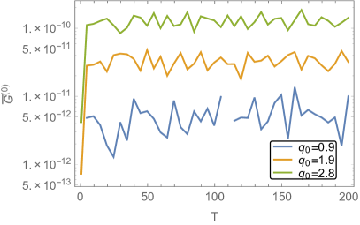
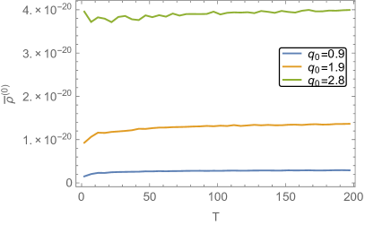
(a) Left graph: $\bar{G}^{(0)}$ as a function of time during the first 200 oscillations of the inflaton field. Right graph: $\bar{\rho}^{0}$ during the first 100 oscillations. $\bar{G}^{(0)}$ and $\bar{\rho}^{(0)}$ are plotted for $q_{0}=0.9$ (blue), $q_{0}=1.9$ (orange) and $q_{0}=2.8$ (green). The quantities are sampled with $\delta T=5$, for values of $T$ where the vacuum dependence is minimal.

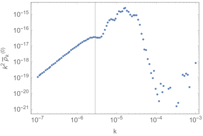
(b) $k^{2}\bar{\rho}_{k}^{(0)}$ as a function of $k$ at $T=3.5$ for $q_{0}=0.9$ (left graph) and $q_{0}=3.7$ (right graph). The vertical line indicates the value of $k_{\text{tach}}$.

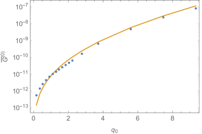
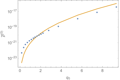
(c) Left graph: comparison between the numerically computed values of $\bar{G}^{(0)}$ (blue) and estimate (50) (orange) as a function of $q_{0}$. $\bar{G}^{(0)}$ was computed after 1.5 oscillations, except for the two largest values of $q_{0}$, where it was computed after 3 oscillations. Right graph: comparison between the numerically computed values of $\bar{\rho}^{(0)}$ (blue) and estimate (53) (orange) as a function of $q_{0}$. $\bar{\rho}^{(0)}$ was computed after 3.5 oscillations.

Figure 1:

4.1 Green function

For small enough comoving momentum $k$ the frequency squared $\omega_{k}^{2}$ of the Higgs modes oscillates between positive and negative values. Modes for which the frequency squared is negative are produced in a process called tachyonic preheating [19, 20]. Modes for which the frequency is non-adiabatic are produced in a process called parametric resonance [16, 17, 18]. Most quanta are produced in the first few oscillations.

We will estimate the contribution of the tachyonic and non-adiabatic modes to the Green function, guided by the numerical results. The first step is to write the mode equation (21) in the form of the Mathieu equation. To do so we approximate the inflaton field and its derivative during the first oscillation as

$$\chi\approx A(T)\cos(2\pi T),\quad\partial_{T}\chi\approx A(T)\partial_{T}\cos(2\pi T),$$ (43)

that is, we neglect the time-dependence of the amplitude in taking the derivative. If furthermore the time-derivative of the mode function is approximated by $\partial^{2}_{\tau}U_{k}\approx(am_{\chi}/(2\pi))^{2}\partial^{2}_{T}U_{k}$, the mode equation (21) can be written in the form of a Mathieu equation:

$$\partial^{2}_{z}U_{k}+\left(\mathcal{A}_{k}-2q\cos(2z)\right)U_{k}=0,$$ (44)

with

$$\mathcal{A}_{k}(T)=\frac{k^{2}}{a^{2}m_{\chi}^{2}}+\frac{1}{2}\hat{\xi}A^{2},\quad q(T)=\frac{3}{4}\hat{\xi}A^{2},\quad 2z=4\pi T-\pi.$$ (45)

Note that the amplitude $A$, scale factor $a$, and thus the parameters $\mathcal{A}_{k},\,q$ are time-dependent in the expanding universe. We define the efficiency parameter as the $q$-value at the initial time

$$q_{0}\equiv q(0)=\frac{3}{4}\hat{\xi}A_{0}^{2}.$$ (46)

Let’s look at tachyonic preheating first. The small momentum modes are tachyonic $\omega_{k}^{2}<0$ during part of the inflaton oscillation. The frequency is most negative at times $T\approx T_{p}=\frac{1}{4}+\frac{1}{2}p$, with $p$ integer. It was estimated in [20] that during the $p$th burst of tachyonic particle production, the tachyonic mode functions grow approximately as:

$$|U_{k}(T_{p})|^{2}\sim\left(\frac{2\omega_{k,0}}{\omega_{k}}\right){\rm e}^{4x\sqrt{q_{p}}},$$ (47)

with $x$ an order one constant. Since $q$ decreases with time, the production is dominated by the first few times the frequency becomes tachyonic. Consider then the first burst of particle production at $T_{p=0}=1/4$. Modes with $k\lesssim k_{\rm tach}$ are tachyonic at that time, with

$$k_{\rm tach}=\frac{2}{\sqrt{3}}a_{1/4}m_{\chi}\sqrt{q_{1/4}},$$ (48)

where we introduced the shorthand $q_{1/4}=q(T=1/4)$ and analogous notation for other time-dependent quantities. The first burst of production gives a contribution to the Green function (34)

$$\bar{G}^{(0)}(1/4) \sim\int^{k_{\rm tach}}\frac{{\rm d}^{3}k}{(2\pi)^{3}2\omega_{k,0}}|U_{k}(1/4)|^{2}\sim\frac{1}{2\pi^{2}}\int^{k_{\rm tach}}{\rm d}k\,k{\rm e}^{4x\sqrt{q_{1/4}}}\sim\frac{1}{2\pi^{2}}k^{2}_{\rm tach}{\rm e}^{4x\sqrt{q_{1/4}}}.$$ (49)

Here we used that the integral is dominated by the modes with $k\sim k_{\rm tach}$, for which the approximation $\omega_{k}\sim k$ is valid. Particle production in the subsequent tachyonic intervals is subdominant. It follows that $\bar{G}^{(n)}$ approaches its asymptotic value after about one inflaton oscillation, and remains constant after that. The above approximation for the Green function is thus valid at large times as well. Relating $q_{1/4}=(A_{1/4}/A_{0})^{2}q_{0}$, the contribution of the tachyonic modes to the Green function can be approximated by:

$$\bar{G}^{(0)}(T)\sim\frac{1}{2\pi^{2}}k^{2}_{\rm tach}{\rm e}^{4x\sqrt{q_{1/4}}}\sim 5\times 10^{-13}q_{0}{\rm e}^{c\sqrt{q_{0}}},$$ (50)

where in the 2nd step we used $m_{\chi}=10^{-5}$ and (3), and defined $c=4x\sqrt{q_{4}/q_{0}}$.

We fit the growth factor $c$ to the numerical results

$$c\approx 3.5.$$ (51)

The left panel of figure 1(c) shows a comparison between the numerically computed values of $\bar{G}^{(0)}$ and approximation (50). The approximation agrees with the numerical result within a factor of two over the whole range $q_{0}=0.15-9.3$, corresponding to $\xi=1-50$. The left panel of figure 1(a) shows the large time behavior of the Green function in the zeroth order adiabatic vacuum. The graphs show that $\bar{G}^{(0)}$ remains approximately constant after the initial amplification, confirming our assumption that production is completely dominated by the first few oscillations.

4.2 Energy density

Analogously to the Green function, the energy density is produced in the first few oscillations and remains constant afterwards, as confirmed by the numerical results shown in Figure 1(a).

The contribution of the tachyonic modes to (35) is estimated as

$$\bar{\rho}^{(0)}(T) \sim\frac{1}{8\pi^{2}}\int^{k_{\rm tach}}kdk\,\left\{|U^{\prime}_{k}|^{2}+\omega_{k}^{2}|U_{k}|^{2}\right\}\Big{|}_{T=\frac{1}{4}}\sim\frac{1}{4\pi^{2}}\int^{k_{\rm tach}}k^{3}dk\,|U_{k}(1/4)|^{2}$$

$$\sim\frac{1}{4\pi^{2}}k_{\rm tach}^{4}{\rm e}^{c\sqrt{q_{0}}}.$$ (52)

In the 2nd step we used that the modes $k\sim k_{\rm tach}$ dominate the integral, analogously to the approximation made in the Green function. Moreover, we assumed equipartition and used $|U^{\prime}_{k}|^{2}\sim k^{2}|U_{k}|^{2}$, which agrees with the numerical results.

Numerically, we fit

$$\bar{\rho}^{(0)}\sim 2.8\times 10^{-23}q_{0}^{2}{\rm e}^{c\sqrt{q_{0}}},$$ (53)

which is about a factor $15$ larger than the contribution from the tachyonic modes (52). The growth factor $c$ is given by (51). This indicates that the energy density and Green function are dominated by the same mode functions.

In the right panel of figure 1(c) a comparison between the numerically computed values of $\bar{\rho}^{(0)}$ after $3.5$ inflaton oscillations and approximation (53) is shown. For $q_{0}>2$ the estimate and numerical result agree within a factor of two, but for smaller $q_{0}$ estimate (53) underestimates the numerical result by a larger margin.

There are several effects that can explain the factor 15 difference between the analytic and numerical result. First of all, the approximation $\omega_{k}\approx k$ could be slightly off. Secondly, the assumption that the production of modes after the first oscillation is negligible does not completely hold for larger $q_{0}$. Furthermore, we did not take into account the contribution of non-tachyonic modes. Figure 1(b) shows $k^{2}\bar{\rho}_{k}^{(0)}$ as a function of $k$ at $T=3.5$. As expected, the resonance is most efficient for the larger value of $q_{0}$. The right graph shows that for $q_{0}=3.7$ the distribution is peaked at a $k_{*}$ that is slightly larger than $k_{\text{tach}}$. The left graph shows that for $q_{0}=0.9$ the difference between $k_{\text{tach}}$ and the most dominant mode $k_{*}$ is approximately a factor 5. This implies that there is a significant contribution of modes that are non-adiabatic, but never tachyonic. This leads to the conclusion that for $q_{0}\lesssim 1$, parametric resonance as described in [17] plays a role that is more important than tachyonic resonance.

These three effects should in principle also apply to our estimate of $\bar{G}^{(0)}$. However, we did not need any multiplicative factor for our fit of $\bar{G}^{(0)}$, which suggests that the effects cancel in this case.

5 Adiabaticity and vacuum dependence

The adiabatic vacuum is a good vacuum for high-momentum modes, for which the adiabaticity parameters defined in (28) are small at least during part of the inflaton oscillation. However, for smaller momenta, adiabaticity is violated at all times. If these momenta give a significant contribution to the Green function and/or energy density, this introduces a large vacuum dependence, which manifests itself in that different orders of adiabatic vacuum give different results for $\bar{G}$ and $\bar{\rho}$.

The adiabatic vacua are all equivalent in the asymptotic time regions where $\omega_{k}$ is (approximately) constant, but can differ significantly during preheating. Since different choices of vacua correspond to different subtractions in $\bar{G}$ and $\bar{\rho}$, see equations (34, 35), they correspond to different counterterms and renormalization conditions. There is thus an uncertainty in the values of the renormalized couplings, which can only be fixed (in theory) by a measurement during preheating. Moreover, even if such a measurement was in principle possible, one would also need to use non-adiabatic methods to calculate the Green function for the results to be useful. Note that the physics is independent of our choice of vacuum, the electroweak vacuum is either stable or not. The problem lies in our theoretical description of this process.

In this section we will discuss the adiabaticity condition and the vacuum dependence of the Green function and energy density, which are both input to determine the stability of the vacuum, as laid out in section 6.1.

5.1 Adiabaticity conditions

After a few oscillations the inflaton background is very well approximated by expression (9). The frequency for the Higgs modes (21) becomes

$$\omega_{k}^{2}\simeq k^{2}+\frac{1}{2}A_{T}^{2}a_{T}^{2}m_{\chi}^{2}\hat{\xi}T^{-2/3}\left(1+3\cos(4\pi T)\right)+\mathcal{O}(T^{-5/3}).$$ (54)

The frequency is periodic with $\delta T=1/2$. In the rest of this section we will use the notation $T{\hat{=}}1/4$ to denote $T=1/4$ mod $1/2$.

Modes with $k<k_{n}$ violate the $n$th-order adiabaticity condition $\epsilon_{n}>1$, which involves $n$ derivatives of the frequency. Keeping only the leading term at large $T$ this gives the estimate

$$k_{n}\sim a_{T}m_{\chi}\left(4\times 2^{(n-2)}\left(\frac{A_{T}}{A_{0}}\right)^{2}q_{0}\right)^{\frac{1}{(n+2)}}T^{\frac{2(n-1)}{3(n+2)}}\times\left\{\begin{array}[]{ll}|\sin(4\pi T)|^{\frac{1}{(n+2)}},&n\;{\rm odd},\\ |\cos(4\pi T)|^{\frac{1}{(n+2)}},&n\;{\rm even},\end{array}\right.$$ (55)

with $A_{T}/A_{0}\approx 0.2$, see (3). Since even orders are proportional to a cosine, and odd orders to a sine, $k_{n}$ cannot be minimized simultaneously for all $n$. At every moment during the inflaton oscillations there are modes that violate some of the adiabaticity conditions. The momentum cutoff $k_{n}$ grows, and as time goes by more modes become non-adiabatic. At early times all $k_{n}$ are similar for $q_{0}=1-10$, but the larger the order $n$ the faster $k_{n}$ grows with time. Explicitly, parametrizing $k_{n}\propto T^{\alpha}$ this gives $\alpha=\{0,1/6,4/15,1/3\}$ for $n=\{1,2,3,4\}$.

The left top plot in fig. 2(a) shows the exact critical $k_{n}$ for which $\epsilon_{n}=1$ (using (9) as the inflaton background) for $n=1,..,4$ during a time interval $\delta T=1/2$; this is compared with our approximation (55) . The approximation is good (it becomes more accurate with larger $T$), except for parts close to the critical points $T{\hat{=}}3/8,1/2,5/8$ where either the sine or the cosine goes to zero.

For the above estimate we only included the classical contribution to the effective mass (41). Taking into account the quantum correction, even if larger than the tree-level term, will have negligible effect. As discussed in the previous subsection $\bar{G}$ is nearly constant at late times, and the time-derivative of $\omega_{k}$ is still given by the time-derivative of the tree-level term. Further, for the $q_{0}$ values of interest $k_{n}^{2}>M_{\rm eff}^{2}$, and one can use the approximation $\omega_{k}\sim k$; the backreaction will not change this either.

If we compare the non-adiabatic modes with the tachyonic modes (48), we see that $k_{\rm tach}<k_{n}$. The tachyonic modes give a an exponentially enhanced contribution to the Green function and energy density, signifying particle production. The larger the enhancement, i.e., the larger $q_{0}$, the smaller the effect of the different adiabatic subtractions. However, since $k_{n}$ grows with time, at sufficiently late times the vacuum dependence of $\bar{G}$ and $\bar{\rho}$ always become substantial. This is what we will discuss next.

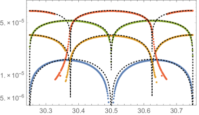
(a) Vacuum dependence. The top left plot shows $k_{n}$ for which $\epsilon_{n}=1$ during a time interval $\delta T=1/2$. The blue, orange, green and red line corresponds to $n=1,2,3,4$ respectively, and the black dotted lines the analytical approximation (55). The right plot shows $\Delta\bar{G}^{(n)}$; the blue, orange and green points correspond to $n=2,4,6$. Only points with ${\rm Im}(\Delta\bar{G}^{(n)})<0.01{\rm Re}(\Delta\bar{G}^{(n)})$ are shown. The black dotted lines correspond to the approximation (58).

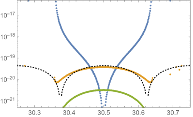
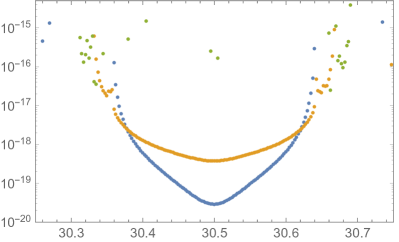
(b) The left plot shows $(2\pi)^{2}\Delta\bar{\rho}^{(2)}_{i}$, blue, orange, and green lines are for $i=1,2,3$ respectively, and the black dotted lines correspond to (61, 61). The right plot shows $\delta\rho^{(n)}$; the blue, orange and green points correspond to $n=2,4,6$. Only points with ${\rm Im}(\bar{\rho}^{(n)})>0.01{\rm Re}(\Delta\bar{\rho}^{(n)})$ are shown. All plots are for $\hat{\xi}=10$.

Figure 2:

5.2 Green function

We now approximate the vacuum dependence of the Green function. The adiabatic frequency is very schematically of the form

$$\left(W_{k}^{(2m)}\right)^{2}=\omega_{k}^{2}+f^{(2m)}(\epsilon_{1},\epsilon_{2},...,\epsilon_{2m}),$$ (56)

that is, $f^{(2m)}$ contains terms up to $2m$ derivatives of the frequency $\omega_{k}$. The highest derivative term dominates, and thus $W^{(2m)}>W^{(2m-2)}$ for modes $k<k_{2m}$ for which $\epsilon_{2m}>1$. Consider the difference between the Green functions of the zeroth and $n$th order adiabatic vacuum. This is approximately

$$\Delta\bar{G}^{(2m)} \equiv\bar{G}^{(2m)}-\bar{G}^{(0)}=\int\frac{d^{3}k}{(2\pi)^{3}}\left(\frac{1}{2W_{k}^{(0)}}-\frac{1}{2W_{k}^{(2m)}}\right)\approx\frac{1}{4\pi^{2}}\int^{k_{2m}}{\rm d}k\,\frac{k^{2}}{W^{(0)}_{k}}$$

$$\sim\frac{1}{8\pi^{2}}k_{2m}^{2}$$ (57)

In the last step we used that $W^{(0)}_{k}=\omega_{k}\sim k$, which is a good approximation for the modes that dominate the integral. Comparing with the exact result, we can fit the constant of proportionality

$$\Delta\bar{G}^{(2)}\approx\frac{1}{8\sqrt{2}\pi^{2}}k_{2}^{2},\quad\Delta\bar{G}^{(4)}\approx\frac{1}{16\pi^{2}}k_{4}^{2},\quad\Delta\bar{G}^{(6)}\approx\frac{1}{16\sqrt{2}\pi^{2}}k_{6}^{2}.$$ (58)

The top right plot in figure 2(a) shows the exact $\Delta\bar{G}^{(n)}$ for $n=2,4,6$ and our approximation (58) over a time interval $\delta T=1/2$. We only show points for which the imaginary part of $\Delta\bar{G}^{(n)}$ is less than 1%. That is, the modes that dominate the integral are all non-tachyonic $W^{(n)}_{k}>0$ and the adiabatic vacuum is defined for them, but we allow that a fraction of the smaller $k$-modes (that give a subdominant contribution) are tachyonic. The vacuum dependence of the Green function grows with time and for larger adiabatic order. However, one cannot take the order to infinity and claim that the vacuum dependence is arbitrarily large, as for larger $n$ the frequency is tachyonic $(W_{k}^{(n)})^{2}<0$ for more $k$-modes and the Green function becomes increasingly less well-defined. Indeed, the plot already shows that for $n=6$ the imaginary part of the Green function exceeds 1% during most of the time interval, also at times where lower order vacua and $\bar{G}^{(2)},\bar{G}^{(4)}$ are still well defined.

The second observation is that the vacuum dependence $\Delta\bar{G}^{(n)}$ is minimized for $T{\hat{=}}1/8,3/8$, in accordance with our estimate (55) as $k_{2m}$ vanishes here. It seems that zooming in on this time instant the vacuum dependence can be made arbitrarily small. However, this is not the case, as in this limit more and more $k$-modes become tachyonic, and at some point the Green function is no longer well defined. This still puts a lower bound on the vacuum dependence. Moreover, at these time instants the frequencies are still non-adiabatic (only the even adiabaticity parameters vanish), and this vanishing is more a coincidence rather than a consequence of adiabaticity. Indeed, as we will see next, the vacuum dependence of the energy density is minimized at different time instants, and one cannot make both of them arbitrarily small at the same time.

5.3 Energy density

Define the vacuum dependence of the energy density via

$$\Delta\bar{\rho}^{(n)}\equiv\bar{\rho}^{(n)}-\bar{\rho}^{(0)},$$ (59)

i.e. we compare the zeroth and $n$th order adiabatic vacuum. To find an analytic approximation it is useful to look at the different terms in $\bar{\rho}_{\rm ad}$ separately

$$\bar{\rho}^{(n)}_{\rm ad} =-\frac{1}{4}\int\frac{d^{3}k}{(2\pi)^{3}}\biggl{\{}\frac{1}{4}\frac{(W_{k}^{(n)^{\prime}})^{2}}{(W^{(n)}_{k})^{3}}+\left(W^{(n)}_{k}+\frac{k^{2}}{W^{(n)}_{k}}\right)+\frac{\hat{\xi}a^{2}R}{W^{(n)}_{k}}\biggr{\}}$$

$$=\bar{\rho}^{(n)}_{1}+\bar{\rho}^{(n)}_{2}+\bar{\rho}^{(n)}_{3}.$$ (60)

For definiteness, concentrate on the $n=2$ vacuum; the results can be generalized to higher order vacua. The term $\Delta\bar{\rho}_{3}$ is subdominant for $T\gtrsim\sqrt{q_{0}}$ and is neglected. The term $\Delta\bar{\rho}_{2}$ is dominated by the modes $k\sim k_{2}$ for which $W^{(0)}\sim W^{(2)}$, and can be estimated by

$$|\Delta\bar{\rho}^{(2)}_{2}|\sim\frac{1}{4\pi^{2}}\int^{k_{2}}{\rm d}k\,k^{2}\times\frac{k}{2}\sim\frac{1}{64\pi^{2}}k_{2}^{4},$$ (61)

where the factor $1/2$ is matched to the numerical solution. The term $\Delta\bar{\rho}_{1}$ is also dominated by modes $k\sim k_{2}$, as the integrand is peaked for these momenta. We estimate

$$|\Delta\bar{\rho}^{(2)}_{1}|\approx\frac{1}{32\pi^{2}}\int^{k_{2}}k^{2}{\rm d}k\,\frac{(W_{k}^{(2)^{\prime}})^{2}}{(W^{(2)}_{k})^{3}}\sim\frac{(W_{k}^{(2)^{\prime}})^{2}\big{|}_{k\sim k_{2}}}{32\pi^{2}(3/2)^{3/2}}\sim\frac{1}{256\sqrt{6}}\frac{k_{3}^{10}}{k_{2}^{6}},$$ (62)

where once again the numerical factors are matched to the numerical solution. It should not surprise that $k_{3}$ enters this estimate, as this term involves an extra time derivative and thus depends on the 3rd adiabaticity parameter.

The different contributions to $\Delta\bar{\rho}^{(2)}$ and the analytical approximation (61, 62) are shown in the bottom left plot in Fig. 2(b). The total vacuum dependence of $\Delta\bar{\rho}^{(n)}$ is shown in the bottom right plot for $n=2,4,6$. Just as for the Green function, only the time instants are shown where the imaginary contribution is less than 1%.

Both approximations agree well with the numerical result away from the critical points $T{\hat{=}}3/8,1/2,5/8$. However, in these limits increasingly more modes become tachyonic, and the energy density is at some point not well defined. The vacuum dependence grows with the order of the vacuum $n$, but just as for the Green function case one cannot take arbitrary large $n$ as these vacua are tachyonic and not defined during most of the time (some of the scattered points, mostly for $\Delta\bar{\rho}^{(6)}$, are a numerical artefact as the integrand behaves wildly for these points).

$\Delta\bar{\rho}^{(n)}$ is minimized for $T{\hat{=}}1/2$ and blows up at the other critical points $T{\hat{=}}3/8,5/8$.

In the following we will use $\bar{G}^{(2)}$ and $\bar{\rho}^{(2)}$ as a an estimate for the vacuum dependence. Away from the critical points to a good approximation

$$\Delta\bar{G}^{(2)}\sim\frac{1}{8\sqrt{2}\pi^{2}}k_{2}^{2},\quad\Delta\bar{\rho}^{(2)}\sim{\rm max}\left[\frac{1}{64\pi^{2}}k_{2}^{4},\,\frac{1}{256\sqrt{6}}\frac{k_{3}^{10}}{k_{2}^{6}}\right].$$ (63)

6 Vacuum stability

In this section we discuss the implications of our results for the vacuum stability. In the next subsection we first discuss the criteria for stability. In 6.2 we analytically determine all the relevant time scales, which (where possible) we compare with the numerical results in 6.3.

6.1 Criteria for stability

The qualitative form of the potential depends sensitively on the Hubble scale. If the Hubble scale is larger than the critical scale $H>\mu_{\rm cr}\sim 10^{11}$GeV it follows from (40) that $\lambda(\mu)<0$ for all Higgs field values $\phi<H$. This is the case at early times, for a sufficiently small number of inflaton oscillations. Using (12) the critical time is given by

$$T_{\rm crit}\sim 25\left(\frac{A_{0}}{0.5}\right)\left(\frac{m_{\chi}}{10^{-5}}\right)\left(\frac{4.2\times 10^{-8}}{\mu_{\rm cr}}\right).$$ (64)

with $A_{0}$ the initial inflaton amplitude. There are then two possibilities for the vacuum to decay.

• The quantum corrections to the effective mass (41) dominate before $T_{\rm crit}$.

  As we have seen the Green function is nearly constant after a few oscillations. As a consequence, if the coupling is negative, the quantum correction to the effective Higgs mass is then always negative. If it exceeds the (oscillating) tree-level contribution the vacuum is destabilized, since there is no barrier. The vacuum can only remain stable if the following criterion is satisfied

  $${\rm\bf condition}\;\;{\bf 1}:\qquad 6\lambda\bar{G}^{\rm ren}(\tau)\lesssim a^{2}\hat{\xi}R_{\text{max}},\quad{\rm for}\;\;T<T_{\rm crit},$$ (65)

  with $R_{\rm max}$ the maximum value of the Ricci scalar during an inflaton oscillation.

• The energy density becomes larger than the potential barrier separating the electroweak and true vacuum.

  If the tree level term dominates the effective mass the potential is an oscillating function with a barrier separating the two vacua. If the quantum correction to the effective mass comes to dominate at late times $T>T_{\rm crit}$, this only enhances the barrier, as the quantum correction to the effective mass is positive at $\phi<\mu_{\rm cr}$.

  The tunnelling process is expected to be enhanced if the energy density in the Higgs modes exceeds the height of barrier, potentially leading to rapid decay. In addition to the first criterion, we thus have a second criterion for vacuum stability:

  $${\rm\bf condition}\;\;{\bf 2}:\hskip 28.45274pt\bar{\rho}^{\rm ren}<\bar{V}_{\text{max}},\hskip 71.13188pt$$ (66)

  with $\bar{V}_{\rm max}$ given in (42).

In the literature, many different criteria for stability are used [23, 24, 25, 26, 27]. Even though the details may differ, all agree that for large non-minimal coupling $q_{0}\gtrsim\mathcal{O}(5)$ particle production is efficient and the electroweak vacuum is destabilized within a couple of inflaton oscillations, since the stability condition (65) is violated.

For smaller couplings particle production is initially not efficient enough to destabilize the vacuum. As the classical background red shift faster than the quantum correction, the energy density may become larger than the effective barrier of the potential at late times, and (66) is violated. However, as we will see, the vacuum dependence of the energy density grows with time, and this makes it hard to make definite statements for small $q_{0}\sim\mathcal{O}(1)$.

6.2 Time scales

In this section we discuss the relevant time scales, starting with some effects we have neglected (inflaton and Higgs decay), and ending with estimates for when the Green function and energy density become large, when the vacuum dependence becomes important, and when the stability criteria are violated.

6.2.1 Inflaton decay

Even though the inflaton decay rate is model dependent, we can make some general statements.

The inflaton oscillates until decay. If it decays via very efficient preheating (into a field other than the Higgs field), the total number of oscillations are $T\lesssim 10^{3}-10^{4}$ [17]. Perturbative decay is slower. The inflaton cannot be coupled too strongly to other fields, as otherwise loop corrections would spoil the flatness of the potential. This gives a bound $T\gtrsim 10^{6}$ corresponding to a maximum reheating temperature $T_{R}\lesssim 10^{12}$GeV; but the number of oscillations can be much larger, for example if the coupling is of gravitational strength and $\Gamma_{\chi}\sim m_{\chi}^{3}/m_{\rm P}^{2}$, decay happens after $T\sim 10^{9}$ oscillations, with a maximum reheating temperature $T_{R}\lesssim 7\times 10^{10}$GeV.

After inflaton decay the universe is dominated by a relativistic fluid, and $R\approx 0$. The classical contribution to the Higgs mass vanishes. However, already before complete decay, there are temperature corrections to both the Higgs mass and the energy density, just like the non-thermal preheating corrections discussed in this paper. The net effect is that the thermal corrections generically stabilize the vacuum — see [8, 14] for the exact bounds. For non-perturbative decay, there is an intermediate non-thermal stage before thermal equilibrium is reached; during this stage the Ricci scalar is non-vanishing. Although a dedicated study will be needed to determine the exact bounds in this case, it is likely that perturbative inflaton decay also helps to stabilize the vacuum.

In the next subsections we will discuss the critical $q_{0}$ value below which the electroweak vacuum is stable, assuming inflaton decay is late and only happens after all relevant time-scales. Since inflaton decay generically stabilizes the electroweak vacuum, fast decay can only raise the critical $q_{0}$ value.

6.2.2 Higgs decay

In coordinate time the Higgs decays when $\Gamma\sim H$, provided decay is kinematically allowed. Translated to conformal time, the condition for decay is

$$aH\sim\alpha M_{\rm eff},$$ (67)

with $\alpha=y^{2}/(4\pi)$ and $y$ a yukawa/gauge coupling. For the top quark and gauge couplings $\alpha\sim(1-5)\times 10^{-2}$ at scales $\mu_{\rm cr}$, and for the bottom quark, tau and Higgs self coupling $\alpha\sim 10^{-4}-10^{-5}$. The fermion/gauge boson mass in conformal time, the equivalent of $M_{\rm eff}$ for the Higgs field (41), only has a contribution from the Higgs fluctuations $M_{y}\sim y^{2}\bar{G}$. Averaged over one oscillation $H^{2}\sim R\sim A^{2}m_{\chi}^{2}/a^{3}$, as follows from (12).

Consider first the case that the tree-level term dominates the Higgs mass $M_{\rm eff}$. The Higgs is much heavier than the SM particles, and decay into top quarks and gauge bosons is kinematically possible. Decay only happens for $\sqrt{\xi}\alpha>1$, so only for large couplings $\xi\gtrsim 10^{4}$.

In the opposite limit that quantum corrections dominate the Higgs mass, decay is kinematically allowed if $M_{\rm eff}>2M_{y}$. Since both the mass of the Higgs and the mass of the decay products scale with $\sqrt{\bar{G}}$, decay into top quark and EW gauge bosons is impossible. Decay into lighter fields is still allowed, in particular decay into b-quarks, tau-leptons and Higgs will dominate. The Higgs decays when

$$\frac{\lambda\bar{G}}{a^{2}\xi R}\gtrsim\frac{1}{\alpha^{2}\xi}\gtrsim\frac{10^{8}}{\xi},$$ (68)

where we used $\alpha\lesssim 10^{-4}$ in the last step.

Perturbative Higgs decay only happens at late times for the $\xi$ couplings of interest, and can be neglected for our purposes.

6.2.3 Large Green function corrections

At late times the maximum value of the classical mass during an oscillation can be approximated by

$$M_{\rm eff}^{2}|_{\rm class}=a^{2}\hat{\xi}R|_{\rm max}=2A_{T}^{2}a_{T}^{2}m_{\chi}^{2}\hat{\xi}T^{-\frac{2}{3}}+\mathcal{O}(T^{-\frac{5}{2}}),$$ (69)

where we used (12). The quantum contribution to the mass $M_{\rm eff}^{2}|_{\rm quant}=6|\lambda|\bar{G}$ becomes of the same order as the classical contribution at time

$$T_{\rm G}\approx 5\times 10^{5}\left(\frac{10^{-2}}{\lambda}\right)^{3/2}{\rm e}^{-\frac{3}{2}c\sqrt{q_{0}}},$$ (70)

where we used (50), and $c$ is given in (51). We find $T_{G}\approx\{4\times 10^{3},\,7\times 10^{2},\,13,\,0.2\}$ for $q_{0}=\{1,\,2,\,5,\,10\}$. Preheating is efficient and the vacuum is destabilized if the quantum correction dominates already when $H>\mu_{\rm cr}$, see our first stability condition (65). This requires $T_{G}<T_{\rm crit}$, with $T_{\rm crit}$ given in (64):

$$T_{\rm G}\lesssim T_{\rm crit}\quad\Rightarrow\quad q_{0}\gtrsim q_{0}^{\rm crit}=4.5\;\;({\rm or}\;\xi\gtrsim 24).$$ (71)

This is reasonably close to the value $q_{0}^{\text{crit}}\approx 3.7$ that we find numerically.

6.2.4 Large energy density

For $T>T_{\rm crit}$ the potential always has a barrier; decay may still be possible if the energy density exceeds the maximum of the potential, see our second stability condition (66). The interesting parameter region is $q_{0}<q_{0}^{\rm crit}$. In that case the energy density becomes large at a time

$$T_{\rho}\sim 2\times 10^{3}{\rm e}^{-\frac{3}{4}c\sqrt{q_{0}}}\left(\frac{10^{-2}}{|\lambda|}\right)^{3/4},$$ (72)

where we used approximation (53). The energy density becomes large before the quantum correction to the Green function becomes large, that is $T_{\rho}<T_{G}$, and the above time-scale was derived using the tree-level potential. Taking $|\lambda|=10^{-2}$, $T_{\rho}\approx\{2\times 10^{2},\,55,\,6,\,0.8\}$ for $q_{0}=\{1,\,2,\,5,\,10\}$.

6.2.5 Vacuum dependence large

We focus on the difference between the 0th and 2nd order adiabatic vacuum, as a measure of the vacuum dependence of the results. The vacuum dependence becomes of the same order as the Green function itself if

$$\frac{\Delta\bar{G}^{(2)}}{\bar{G}^{(0)}}>1\quad\Rightarrow\quad T>T_{\Delta G}=6\times 10^{-3}q_{0}^{3/2}{\rm e}^{3c\sqrt{q_{0}}},$$ (73)

where we took $\cos(4\pi T)\sim 1$. This gives $T_{\Delta G}=\{80,\,10^{5},\,10^{8}\}$ for $q_{0}=\{1,\,2,\,5\}$. $T_{\Delta G}<1$ for $q_{0}<1$. The Green function enters the first stability criterion (65) for effective preheating, which is valid if the vacuum decays within the first $~{}25$ oscillations and $q_{0}>q_{0}^{\rm crit}=4.5$. It follows from (73) that the vacuum dependence of the results is small in this case.

If we compute the energy density at the instants where the vacuum dependence is minimized $T\hat{=}\frac{1}{2}$, we have $\Delta\bar{\rho}^{(2)}=\frac{1}{64\pi^{2}}k_{2}^{4}$ and the vacuum dependence of the energy density becomes sizeable when

$$\frac{\Delta\bar{\rho}^{(2)}}{\bar{\rho}^{(0)}}>1\quad\Rightarrow\quad T>T_{\Delta\rho}=0.21e^{\frac{3}{2}c\sqrt{q_{0}}}q_{0}^{2}.$$ (74)

This gives $T_{\Delta\rho}\approx\{40,\,10^{3},\,3\times 10^{5}\}$ for $q_{0}=\{1,\,2,\,5\}$. The energy density enters the second stability criterion (66) for $q_{0}<q_{0}^{\rm crit}$. Demanding that

$$T_{\rho}<T_{\Delta\rho}\quad\Rightarrow\quad q_{0}\gtrsim 1.3\quad({\rm or}\;\xi\gtrsim 7).$$ (75)

However, $V_{\rm max}$, $\bar{\rho}$ and $\Delta\bar{\rho}$ are all oscillating functions. We can not expect that an interpolation between the points where the vacuum dependence of $\bar{\rho}$ is minimized gives a proper description of $\bar{\rho}$ during the whole oscillation, or of the oscillation averaged $\bar{\rho}$. For an accurate determination of the tunneling rate to the true vacuum, information at other time instants may be needed.

Moving slightly away from $T\hat{=}\frac{1}{2}$, the vacuum dependence is given by $\Delta\bar{\rho}^{2}=\frac{1}{256\sqrt{6}}\frac{k_{3}^{10}}{k_{2}^{6}}$ and $T_{\Delta\rho}$ becomes much smaller. Taking $T\hat{=}\frac{1}{2}+0.05$ as an example, we get:

$$\frac{\Delta\bar{\rho}^{(2)}}{\bar{\rho}^{(0)}}>1\quad\Rightarrow\quad T>T_{\Delta\rho}=0.27e^{\frac{3}{5}c\sqrt{q_{0}}}q_{0}^{9/10},$$ (76)

which gives $T_{\Delta\rho}\approx\{2,\,10,\,10^{2}\}$ for $q_{0}=\{1,\,2,\,5\}$. Demanding again that $T_{\rho}<T_{\Delta\rho}$ gives the stronger bound

$$T_{\rho}<T_{\Delta\rho}\quad\Rightarrow\quad q_{0}\gtrsim 2.8\quad({\rm or}\;\xi\gtrsim 15).$$ (77)

Numerically we find $q_{0}\sim 0.9$ (or $\xi\sim 5$) when we look at the vacuum dependence at $T\hat{=}\frac{1}{2}$, and $q_{0}\sim 2.2$ (or $\xi\sim 12$) for $T\hat{=}\frac{1}{2}+0.05$.

6.3 Numerical results

In this section we present the results of our numerical calculation, which serves as a check for the analytical results discussed in the previous sections. We focus on the calculation of the Higgs Green function and energy density, and in particular on their vacuum dependence by calculating them in both the zeroth and second order vacuum (31).

6.3.1 Numerical implementation

Since our aim is not so much on getting the most accurate results, but rather on investigating the vacuum dependence, we have made some simplifying assumptions to speed up the numerics.

First of all, we neglect the Higgs mass term and quartic Higgs coupling. The electroweak scale mass is negligible during preheating. The quartic coupling only becomes important near the maximum of the potential, but can be neglected for smaller field values. Since we are only interested in the question whether the EW vacuum is destabilized, and not in the exact dynamics of the Higgs after crossing the barrier, we can neglect this interaction. This is supported by numerical simulations in the literature (see e.g. [24]).

Secondly, we neglect backreaction. It can be checked that the backreaction on the inflaton equation of motion of the produced particles is small. The backreaction for the Higgs mode equation becomes important once the barrier disappears and $M^{2}_{\rm eff}$ becomes negative (41). At this point the vacuum is already destabilized.

Thirdly, we neglect the interaction of the Higgs with all other SM particles and also other inflaton interactions (which should be there for complete decay of the inflaton). As will be discussed in 6.2, Higgs decay happens on large time-scales and can be neglected; inflaton decay is model dependent, but is expected to only increase stability.

Since the inflaton background is formulated in coordinate time (7), we solve for the Higgs modes in coordinate time as well. The mode functions satisfy the differential equation:

$$\ddot{U}_{k}+H\dot{U}_{k}+\frac{\omega_{k}^{2}}{a^{2}}U_{k}=0,\qquad\omega_{k}^{2}=k^{2}+a^{2}(\xi-\frac{1}{6})R.$$ (78)

As suggested in [36], we write the mode functions as

$$U_{k}=e^{-i\omega_{k,0}\tau}(1+h_{k}),\qquad h_{k}(t_{0})=\dot{h}_{k}(t_{0})=0.$$ (79)

These $h_{k}$-functions satisfy the mode equation:

$$\ddot{h}_{k}+\left(H-\frac{2i\omega_{k,0}}{a}\right)\dot{h}_{k}=-\left(\xi-\frac{1}{6}\right)\left(R-\frac{a^{2}(t_{0})}{a^{2}}R(t_{0})\right)(1+h_{k}).$$ (80)

The mode equations are solved numerically in Mathematica. The $h_{k}$-modes are numerically more stable for large $k$ than the $U_{k}$-modes.

We are interested in the quantities $\bar{\rho}^{(n)}$ and $\bar{G}^{(n)}$, which are obtained by integrating over $U_{k}$-modes. In order to keep the computation time manageable, the integral is replaced by a sum. Typically we compute $U_{k}$ and $\dot{U}_{k}$ for 100 values of $k$ lying on a logarithmic scale between $10^{-7}$ and $10^{-3}$. The mode functions do not vary significantly with $k$ for $k$ as small as $10^{-7}$. Furthermore, the contribution for small $k$ is suppressed by the factor $k^{2}$ from the Jacobian, so our lower boundary is effectively zero. The contribution of the large $k$ modes decreases exponentially beyond a certain cutoff (much smaller than $k=10^{-3}$), due to the adiabatic renormalization, and these modes can be neglected.

Since we use the adiabatic approximation for renormalization, our expressions for $\bar{\rho}$ and $\bar{G}$ are only properly defined when $W_{k}^{2}(t)>0$. In order to have a continuous graph, we either interpolate between values of $T$ for which $W_{k}^{2}(t)>0$ when we focus on large time scales, or, when we focus on shorter time scales, we take the absolute value of the renormalization terms in equation (34). We sample

6.3.2 Results

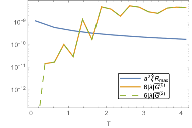
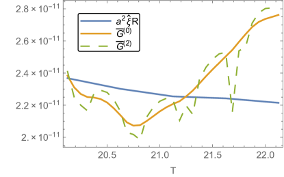
(a) Left: $q_{0}=9.3$. Tree-level contribution $a^{2}\hat{\xi}R$ (blue) and one-loop contribution $6|\lambda|\bar{G}$ (orange and green) to the effective Higgs mass for the first few oscillations. The $a^{2}\hat{\xi}R$-term oscillates in reality, but in this graph we show an interpolation between the maxima. The solid orange line shows the result for $\bar{G}$ in the zeroth order adiabatic vacuum, the dashed green line shows the second order result. In order to have a continuous plot, we take the absolute value of the renormalization terms in equation (34). $\bar{G}$ is sampled with $\delta T=1/4$ Right: $q_{0}=3.7$. (Interpolation between the maxima of) tree-level contribution $a^{2}\hat{\xi}R$ (blue) and one-loop contribution $6|\lambda|\bar{G}$ (orange and green) to the effective Higgs mass at $T\approx 21$. The solid orange line shows the result for $\bar{G}$ in the zeroth order adiabatic vacuum, the dashed green line shows the second order result. In order to have a continuous plot, we take the absolute value of the renormalization terms in equation (34). $\bar{G}$ is sampled with $\delta T=1/16$.

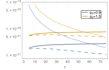
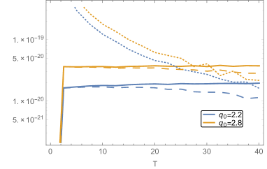
(b) Interpolation of the maxima of $\bar{\rho}$ and $\bar{V}_{\text{max}}$ as a function of time. The solid line shows $\bar{\rho}^{(0)}$, the dashed line shows $\bar{\rho}^{(2)}$, the dotted line shows $\bar{V}_{\text{max}}$ in the zeroth order vacuum (the second order result looks identical). Left: $q_{0}=0.9$ (blue) and $q_{0}=1.5$ (orange). $\bar{\rho}$ and $\bar{V}_{\text{max}}$ are sampled with $\delta T=5$, starting at $T=0$, such that the vacuum dependence is minimized. Right: $q_{0}=2.2$ (blue) and $q_{0}=2.8$ (orange). $\bar{\rho}$ and $\bar{V}_{\text{max}}$ are sampled with $\delta T=2.5$, starting at $T=0.05$.

Figure 3:

Large $q_{0}$, immediate decay of the Higgs

Preheating is efficient for $q_{0}\gg 1$, or equivalently $\xi\gg 1$, and leads to decay of the electroweak vacuum. We show the results for $q_{0}=9.3$ ($\xi=50$) in figure 3(a). We plotted both the oscillating tree-level contribution to the effective Higgs mass and the negative one-loop contribution. Within one inflaton oscillation the latter dominates and the first criterion for stability (65) is violated: the potential does not have a maximum anymore and the Higgs will inevitably roll down to the true minimum. It should be noted that once that happens, our results are inaccurate, since it is no longer justified to neglect the quartic term from the potential. We tested for vacuum dependence, by calculating the quantum correction in both the zeroth and second order adiabatic vacuum (31). Only during the first half of the first oscillation we can see a difference between the zeroth and second order adiabatic renormalization, but the final result is nearly vacuum independent, as expected from equation (73).

Large-$T$ behavior of $\bar{G}$ and $\bar{\rho}$.

For smaller values of $q_{0}$, preheating is less efficient, and the initial production of Higgs modes is not enough to let the Higgs decay within the first few oscillations.

As was shown in figure 1(a), the Green function and energy density remain approximately constant after the initial amplification. Due to the different scaling of the classical and one-loop contribution, the first stability criterion might still be violated before $H$ becomes smaller than the instability scale $\mu_{\text{cr}}$ even if $q_{0}$ was not large enough to lead to immediate Higgs decay.

Figure 3(a) shows the tree level and one-loop mass entering the first stability criterion (65) at $T\approx 21$ for $q_{0}=3.7$ ($\xi=20$). The graph shows that the one-loop contribution indeed becomes larger than the tree-level contribution, resulting in decay of the Higgs. The difference between $\bar{G}$ in the two vacua is approximately 50 times smaller than $\bar{G}$ itself. Since the Hubble constant becomes smaller than $\mu_{\text{cr}}$ around $T=25$, the first criterion for stability will not be violated for values of $q_{0}\lesssim 3.7$. This value of $q_{0}$ is reasonably close to the estimated value of $q_{0}^{\text{crit}}=4.5$.

Comparison of $\bar{V}_{\text{max}}$ and $\bar{\rho}$ for $q_{0}<3.7$.

For $q_{0}<3.7$, the Green function contribution does not become dominant before $T=25$, so we need to look at the second stability criterion (66) to determine the fate of the Higgs.

The left plot of figure 3(b) shows a comparison between $\bar{\rho}^{(0)}$, $\bar{\rho}^{(2)}$ and $\bar{V}_{\text{max}}$ for $q_{0}=0.9,1.5$ ($\xi=5,8$) for values $T\hat{=}\frac{1}{2}$ where the vacuum dependence is minimized. The computation of $\bar{V}_{\text{max}}$ is done in the zeroth order vacuum, but the vacuum dependence of $\bar{V}_{\text{max}}$ is in any case subdominant. For $q_{0}=1.5$, $\bar{\rho}$ becomes comparable to $\bar{V}_{\text{max}}$ when the vacuum dependence is still rather small, implying that there is a possibility of vacuum decay (remember though that $\bar{\rho}$ oscillates). For $q_{0}=0.9$, $\Delta\bar{\rho}^{(2)}$ becomes comparable to $\bar{\rho}^{0}$ at the same time when $\bar{\rho}^{(0)}=\bar{V}_{\text{max}}$. As a consequence, we can not determine whether the Higgs decays. Our critical value of $q_{0}$ agrees reasonably well with the estimated value of $q_{0}\approx 1.3$. We conclude that for $q_{0}\lesssim 0.9$ (or $\xi\lesssim 12$) we can not draw vacuum-independent conclusions about the stability of the Higgs.

The right graph of figure 3(b) gives an even stricter bound on the value of $q_{0}$ for which vacuum-independent statements can be made. $\bar{\rho}$ and $\bar{V}_{\text{max}}$ are determined at $T\hat{=}\frac{1}{2}+0.05$. We then find that no vacuum dependent statements can be made for $q_{0}\lesssim 2.2$.

7 Conclusion

In this work we studied the stability of the Higgs field during preheating in the presence of a non-minimal coupling between the Higgs field and the Ricci scalar. After inflation the inflaton oscillates in its potential and the effective Higgs mass squared oscillates between positive and negative values. Higgs modes with momentum $k$ such that $\omega_{k}^{2}<0$ during part of the inflaton oscillation are produced in a process called tachyonic preheating; in addition non-adiabatic modes are produced n a process called parametric resonance. The produced Higgs modes contribute to the effective potential and the energy density.

Vacuum decay can now occur in two ways. First, if preheating is very efficient it leads to explosive particle production and within a few oscillations the effective Higgs mass is dominated by the one-loop corrections. At early times the Hubble exceeds the critical renormalization scale and the Higgs coupling is negative $\lambda(\mu\sim H)<0$, and consequently the effective Higgs mass is negative. The Higgs will inevitably roll down to the true minimum. Secondly, if preheating is less efficient, the one-loop contribution may still dominate at late times as the background term red shifts away faster. At late times and for smaller Hubble scale, the effective potential will always have a barrier separating the true and false vacuum. However, the energy density may become comparable or larger than the maximum of the potential, making tunnelling to the true vacuum likely.

Particle production is dominated by the initial times, where the Higgs mass becomes most negative. This allows to approximate the Green function and energy density by the contribution during the first oscillation, as it remains (nearly) constant afterwards. We presented the semi-analytic approximations in section 4. We compared the analytical estimate of the propagator and energy density with the numerical values for values of the efficiency parameter $q_{0}$ between $0.16$ and $9.3$ ($\xi$ between 1 and 50) and found an agreement up to a factor of 2 for most values of $q_{0}$.

The results are defined with respect to the $n$th order adiabatic vacuum. The adiabatic vacuum is a good vacuum for high momentum modes, for which the adiabaticity parameters defined in (28) are small at least during part of the inflaton oscillation. However, for smaller momenta, adiabaticity is always violated. We found that the contribution of the non-adiabatic momenta to the Green function and/or energy density grows with time, and thus the vacuum dependence grows with time. Since different choices of vacua correspond to different renormalization conditions, there is thus an uncertainty in the values of the renormalized couplings — and in the definition of the critical coupling for vacuum stability — which can only be fixed (in theory) by a measurement during preheating.

Our main results are that for $q_{0}\gtrsim 3.7$ preheating is efficient and the vacuum decays at early times when $H>\mu_{\rm cr}$. This is in agreement with results in the literature [23, 24, 25, 26, 27]. Since decay is rapid, vacuum effects are negligible in this case.

For $0.9.\lesssim q_{0}\lesssim 3.7$ the Higgs potential always has a barrier, but the energy density becomes of the order of the barrier height before the results are swamped by uncertainties due to the vacuum choice.

For $q_{0}\lesssim 0.9$ however, no definite statements can be made. This bound becomes stricter if we compare $\bar{\rho}$ and $\bar{V}_{\text{max}}$ at time instants where the vacuum dependence of $\bar{\rho}$ is not minimized. When the energy density becomes large enough for the vacuum to be in peril, the vacuum dependence is already large (the difference in energy density for different vacua is larger than the energy density itself calculated in the zeroth order vacuum). As a consequence there is a large uncertainty in the definition of the effective couplings, and thus any attempt to determine a critical coupling for stability is hampered by that. Note that this is arguably the most interesting part of parameter space, as order one couplings and initial conditions such as in chaotic or Starobinsky inflation lead to $q_{0}=\mathcal{O}(1)$.

References

- [1] F. Bezrukov, M. Y. .Kalmykov, B. A. Kniehl and M. Shaposhnikov, JHEP 1210, 140 (2012) [arXiv:1205.2893 [hep-ph]].
- [2] G. Degrassi, S. Di Vita, J. Elias-Miro, J. R. Espinosa, G. F. Giudice, G. Isidori and A. Strumia, JHEP 1208, 098 (2012) [arXiv:1205.6497 [hep-ph]].
- [3] V. Branchina and E. Messina, Phys. Rev. Lett. 111, 241801 (2013) [arXiv:1307.5193 [hep-ph]].
- [4] V. Branchina and E. Messina, arXiv:1507.08812 [hep-ph].
- [5] A. Kobakhidze and A. Spencer-Smith, arXiv:1404.4709 [hep-ph].
- [6] A. Spencer-Smith, arXiv:1405.1975 [hep-ph].
- [7] A. V. Bednyakov, B. A. Kniehl, A. F. Pikelner and O. L. Veretin, arXiv:1507.08833 [hep-ph].
- [8] J. R. Espinosa, G. F. Giudice and A. Riotto, JCAP 0805 (2008) 002 doi:10.1088/1475-7516/2008/05/002 [arXiv:0710.2484 [hep-ph]].
- [9] K. Enqvist, T. Meriniemi and S. Nurmi, JCAP 1407 (2014) 025 doi:10.1088/1475-7516/2014/07/025 [arXiv:1404.3699 [hep-ph]].
- [10] M. Fairbairn and R. Hogan, Phys. Rev. Lett. 112 (2014) 201801 doi:10.1103/PhysRevLett.112.201801 [arXiv:1403.6786 [hep-ph]].
- [11] A. Kobakhidze and A. Spencer-Smith, Phys. Lett. B 722 (2013) 130 doi:10.1016/j.physletb.2013.04.013 [arXiv:1301.2846 [hep-ph]].
- [12] A. Hook, J. Kearney, B. Shakya and K. M. Zurek, JHEP 1501 (2015) 061 doi:10.1007/JHEP01(2015)061 [arXiv:1404.5953 [hep-ph]].
- [13] M. Herranen, T. Markkanen, S. Nurmi and A. Rajantie, Phys. Rev. Lett. 113 (2014) no.21, 211102 doi:10.1103/PhysRevLett.113.211102 [arXiv:1407.3141 [hep-ph]].
- [14] J. R. Espinosa, G. F. Giudice, E. Morgante, A. Riotto, L. Senatore, A. Strumia and N. Tetradis, JHEP 1509 (2015) 174 doi:10.1007/JHEP09(2015)174 [arXiv:1505.04825 [hep-ph]].
- [15] K. Kamada, Phys. Lett. B 742 (2015) 126 doi:10.1016/j.physletb.2015.01.024 [arXiv:1409.5078 [hep-ph]].
- [16] L. Kofman, A. D. Linde and A. A. Starobinsky, Phys. Rev. Lett. 73 (1994) 3195 doi:10.1103/PhysRevLett.73.3195 [hep-th/9405187].
- [17] L. Kofman, A. D. Linde and A. A. Starobinsky, Phys. Rev. D 56 (1997) 3258 doi:10.1103/PhysRevD.56.3258 [hep-ph/9704452].
- [18] Y. Shtanov, J. H. Traschen and R. H. Brandenberger, Phys. Rev. D 51 (1995) 5438 doi:10.1103/PhysRevD.51.5438 [hep-ph/9407247].
- [19] G. N. Felder, J. Garcia-Bellido, P. B. Greene, L. Kofman, A. D. Linde and I. Tkachev, Phys. Rev. Lett. 87 (2001) 011601 doi:10.1103/PhysRevLett.87.011601 [hep-ph/0012142].
- [20] J. F. Dufaux, G. N. Felder, L. Kofman, M. Peloso and D. Podolsky, JCAP 0607 (2006) 006 doi:10.1088/1475-7516/2006/07/006 [hep-ph/0602144].
- [21] S. Tsujikawa, K. i. Maeda and T. Torii, Phys. Rev. D 60 (1999) 063515 doi:10.1103/PhysRevD.60.063515 [hep-ph/9901306].
- [22] B. A. Bassett and S. Liberati, Phys. Rev. D 58 (1998) 021302 Erratum: [Phys. Rev. D 60 (1999) 049902] doi:10.1103/PhysRevD.60.049902, 10.1103/PhysRevD.58.021302 [hep-ph/9709417].
- [23] M. Herranen, T. Markkanen, S. Nurmi and A. Rajantie, Phys. Rev. Lett. 115 (2015) 241301 doi:10.1103/PhysRevLett.115.241301 [arXiv:1506.04065 [hep-ph]].
- [24] Y. Ema, K. Mukaida and K. Nakayama, JCAP 1610 (2016) no.10, 043 doi:10.1088/1475-7516/2016/10/043 [arXiv:1602.00483 [hep-ph]].
- [25] K. Kohri and H. Matsui, Phys. Rev. D 94 (2016) no.10, 103509 doi:10.1103/PhysRevD.94.103509 [arXiv:1602.02100 [hep-ph]].
- [26] K. Kohri and H. Matsui, arXiv:1607.08133 [hep-ph].
- [27] K. Enqvist, M. Karciauskas, O. Lebedev, S. Rusak and M. Zatta, JCAP 1611 (2016) 025 doi:10.1088/1475-7516/2016/11/025 [arXiv:1608.08848 [hep-ph]].
- [28] N. D. Birrell and P. C. W. Davies, doi:10.1017/CBO9780511622632
- [29] L. V. Keldysh, Zh. Eksp. Teor. Fiz. 47 (1964) 1515 [Sov. Phys. JETP 20 (1965) 1018].
- [30] J. S. Schwinger, J. Math. Phys. 2 (1961) 407. doi:10.1063/1.1703727.
- [31] R. D. Jordan, Phys. Rev. D 33 (1986) 444. doi:10.1103/PhysRevD.33.444
- [32] E. Calzetta and B. L. Hu, Phys. Rev. D 35 (1987) 495. doi:10.1103/PhysRevD.35.495
- [33] E. Calzetta and B. L. Hu, Phys. Rev. D 37 (1988) 2878. doi:10.1103/PhysRevD.37.2878
- [34] A. Ringwald, Z. Phys. C 34 (1987) 481. doi:10.1007/BF01679866
- [35] A. Ringwald, Annals Phys. 177 (1987) 129. doi:10.1016/S0003-4916(87)80027-1
- [36] J. Baacke, K. Heitmann and C. Patzold, Phys. Rev. D 56 (1997) 6556 doi:10.1103/PhysRevD.56.6556 [hep-ph/9706274].
- [37] J. Baacke, K. Heitmann and C. Patzold, Phys. Rev. D 55 (1997) 2320 doi:10.1103/PhysRevD.55.2320 [hep-th/9608006].
- [38] L. Parker and S. A. Fulling, Phys. Rev. D 9 (1974) 341. doi:10.1103/PhysRevD.9.341
- [39] S. A. Fulling, L. Parker and B. L. Hu, Phys. Rev. D 10 (1974) 3905. doi:10.1103/PhysRevD.10.3905
- [40] T. S. Bunch, J. Phys. A 13 (1980) 1297. doi:10.1088/0305-4470/13/4/022
- [41] T. Markkanen and A. Tranberg, JCAP 1308 (2013) 045 doi:10.1088/1475-7516/2013/08/045 [arXiv:1303.0180 [hep-th]].
- [42] J. P. Paz and F. D. Mazzitelli, Phys. Rev. D 37 (1988) 2170. doi:10.1103/PhysRevD.37.2170
- [43] V. Mukhanov and S. Winitzki,
- [44] S. R. Coleman and E. J. Weinberg, Phys. Rev. D 7 (1973) 1888. doi:10.1103/PhysRevD.7.1888
- [45] I. G. Moss, arXiv:1509.03554 [hep-th].