Information Management for Decentralized Energy Storages under Market Uncertainties

Abstract

In this paper, we propose a model of decentralized energy storages, who serve as instruments to shift energy supply intertemporally. From storages’ perspective, we investigate their optimal buying or selling decisions under market uncertainty. The goal of this paper is to understand the economic value of future market information, as energy storages mitigate market uncertainty by forward-looking strategies.

At a system level, we evaluate different information management policies to coordinate storages’ actions and improve their aggregate profitability: (1) providing a publicly available market forecasting channel; (2) encouraging decentralized storages to share their private forecasts with each other; (3) releasing additional market information to a targeted subset of storages exclusively. We highlight the perils of too much market information provision and advice on exclusiveness of market forecast channel.

Keywords: Energy storages, energy forecasting, Cournot competition, game with incomplete information.

1 Introduction

Energy storages serve as instruments for energy supply shift by storing excess renewable energy for the future. As the power industry transitions from a regulated towards a more competitive market environment, storage devices have incentives to be charged when prices are low (corresponding to low residual demand), and discharges when prices are higher (peak demand). The economic feasibility of such delicate operations requires optimal utilization of decentralized storage devices, wherein storage devices pursue their own objective (e.g., maximize profits or minimize costs) (Sarker et al. 2015). Tesla Powerwall is among the most renowned examples of such applications (Motors 2016).

The application scenarios we focus on in this paper are when energy storages are integrated with renewable energy (e.g., wind and solar power) generation. For example, energy supply shift is necessary when the peak in solar power supply is during the daytime whereas the peak demand is during the night. In this case, energy storages are placed near the wind and solar power production sites to smooth generation output before connecting to aggregator and feeding to the grid (Grothoff 2015). However, a fundamental problem in this integration is so called “merit order effect”: The supply of renewable energy has negligible marginal costs and in turn reduces the spot equilibrium price (Acemoglu et al. 2015). For example, since the price of power is expected to be lower during periods with high wind than in periods with low wind, the intermittency of renewable energy generation leads to market variability and uncertainty, i.e., energy prices fluctuates dynamically over time.

Facing these challenges, energy storages have to employ market forecasts to improve buying and selling decisions. The goal of this paper is to understand the economic value of future market information, as energy storages mitigate market uncertainty by forward-looking strategies. In particular, we address the following research questions:

• From storages’ perspective, what are the optimal decentralized buying or selling quantities, when the energy prices are both uncertain and variable over time?

• At a system level, what is a good information management policy, to coordinate storages’ actions and improve their profitability?

To be specific, we provide a stylized model of optimal storage planning under private market price forecasting. Decentralized decision makers have to consider their optimal strategies in a competitive environment with strategic interactions. In terms of information management, we consider the following possible policy interventions: (1) providing a publicly available market forecasting channel; (2) encouraging decentralized storages to share their private forecasts with each other; (3) release additional market information to a targeted subset of storages exclusively.

The rest of this paper is organized as follows. Section 2 reviews relevant literature. Section 3 introduces our model setup. In Section 4, we carry out the analysis for two basic (simplified) models. In Section 5, we describe several policy intervention solutions. In Section 6, we extend the basic models in several directions. Section 7 concludes this paper with a discussion of the future research directions.

2 Literature Review

Our work contributes to the literature on oligopoly energy market. The Cournot setup is a good approximation to some energy markets, e.g., California’s electricity industry as has been demonstrated in (Borenstein and Bushnell 1999). Similar empirical work has been done in New Zealand’s electricity markets (Scott and Read 1996). This paper is partly inspired by Acemoglu et al. (2015), wherein they also consider a competitive energy market with highly asymmetric information structures. While they seek to mitigate uncertainty and economic inefficiency via contractual designs, we aim the same target with informational interventions. We also focus on energy storages wherein they consider energy producers.

In terms of energy storage modeling, our model extends a similar work presented in Contreras-Ocana et al. (2015), wherein they assume complete information and deterministic demand function. The fundamental inefficiency of such an energy market is driven by highly volatile local market conditions (e.g. electricity prices), for instance, due to intermittency in the renewable energy supply. For this reason, there is a growing literature on the use of an energy storage system to improve integration of the renewable energy (Dicorato et al. 2012; Shu and Jirutitijaroen 2014). With this motivation (while abstracting away from the physical characteristics of the renewables), our model is closely related to this literature by incorporating both intertemporal variability and uncertainty (exogenous market price shocks). Given such an environment, storages will be foresighted and joint storage planning and forecasting have been reported consequently (Li et al. 2016; Haessig et al. 2015). While this literature is mostly simulation-based, our model admits tractable analysis and interpretable structural results.

Beyond discussions on distributed storage planning and control, we put emphasis on information management at a system level. In a deregulated environment, it is natural to consider that the competing storages do not observe each other’s private information (private energy price forecast). Therefore, the storages have to estimate each other’s private forecast and conjecture on how each other’s action depends on its forecast. This strategic interaction poses technical challenge, which is new to the energy literature. A similar problem is studied in Kamalinia et al. (2014) in a different context (generation capacity expansion), wherein no structural results are available. Li and Shahidehpour (2005) and Langary et al. (2014) touch upon this topic in the context of generating companies’ supply function equilibrium but resort to simulation. Furthermore, the private forecast in our model is sequentially revealed at every periods, while the private information in aforementioned literature is static (viewed as generation companies’ attribute or type).

Finally, there is a long stream of literature in economics and operations research in terms of information management in such a decentralized setting. We consider a class of equilibria wherein each agent’s action depends linearly on its forecast and forms Bayes’ estimator for others’ forecasts. The uniqueness of this equilibrium prediction is guaranteed by Radner (1962). The value of a public forecast in coordinating agents’ actions is pioneered in Morris and Shin (2002). The incentives for information sharing are studied in Gal-Or (1985). A recent work has demonstrated the power of targeted information release Zhou and Chen (2016). We systematically examine those ideas in the context of distributed energy storage market.

3 Model

Market structure. Consider $n$ storages who purchase and sell substitutable energy through a common market. The storages, indexed by a set $I=\{1,2,\cdots,n\}$, are homogeneous ex ante and engage in a Cournot competition. Let $d_{i}^{[t]}$ denote the energy purchased (when $d_{i}^{[t]}<0$) or sold (when $d_{i}^{[t]}>0$) by the $i^{th}$ storage at time $t$, and the aggregate storage quantity is denoted by $D^{[t]}=\sum_{i=1}^{i=n}d_{i}^{[t]}$. We model the demand side by assuming that the actual market clearing price $P^{[t]}(D^{[t]})$ is linear in $D^{[t]}$, i.e.,

$$P^{[t]}(D^{[t]})=\beta^{[t]}-\gamma^{[t]}D^{[t]}+\eta^{[t]},\forall t\in T,$$ (1)

where a random variable $\eta^{[t]}$ captures the market uncertainty. $\beta^{[t]}>0$ corresponds to market potential, which also captures market variability since $\beta^{[t]}$ is changing over time. $\gamma^{[t]}>0$ (price elasticity) captures the fact that the market price decreases when the aggregate energy sold $D^{[t]}$ increases, as the market supply of energy increases.

To model storages’ strategic interactions, our demand side setup corresponds to a scenario wherein storages are not price-takers but enjoy market power. This is supported by empirical evidence that energy prices vary in response to loads generation, especially when the storages are of sufficient scale (Sioshansi et al. 2009). Even if the storages are small-scaled, economics literature suggests that infinitesimal agents also act as if they are expecting the price-supply relationship (Osborne 2005). Similar assumptions on storages’ market power and price-anticipatory behavior are not uncommon in the literature (Sioshansi 2010). Finally, with the integration of renewables and consequently the “merit order effect”, the supply of renewable energy can drastically impact the spot equilibrium price considering its negligible marginal costs.

We assume that the market uncertainty follows an autoregressive process such that

$$\eta^{[t+1]}=\delta\eta^{[t]}+\epsilon_{t},\forall t\in T,\eta^{[1]}\sim N(0,\alpha^{-1}).$$ (2)

The parameter $\alpha$ is the initial information precision concerning the market uncertainty a priori. Standard assumptions for autoregressive process require that $\left|\delta\right|<1$, where $\epsilon_{t}$ is exogenous shock $\epsilon_{t}\sim N(0,\zeta^{-1})$. We choose this stochastic process as it is among the simplest ones which capture intertemporal correlation while remaining realistic.

Storage model. Storages are agents who can buy energy at a certain time period and sell it at another. The net energy purchased and sold across time is required to be zero for every storage, i.e., $\sum_{t\in T}d_{i}^{[t]}=0$, $\forall i\in I$. As we seek to emphasize the interaction between storages, we also abstract away from other operational constraints such as energy and/or power limits; Instead, they are modeled by a cost function associated with each storage. The battery degradation, efficiency, and/or energy transaction costs of storage $i$ are represented by the cost function $c_{i}(\cdot)$. This treatment is similar to that in Contreras-Ocana et al. (2015).

We assume that $c_{i}(d)=\varepsilon^{[t]}\cdot d^{2}$ in the basic models. More realistically, $c_{i}(d)$ will be a power function $\varepsilon^{[t]}\cdot d^{x}$ wherein $x\in(1,2)$, as it is known that as the depth of discharge increases, the costs of utilizing storage increase faster than linear. We can show that most of our results remain robust when the cost function $c_{i}(d)$ is generalized within this region. We choose $x=2$ for a clear presentation of results. We also generalize the basic model to consider heterogeneous cost functions in the extensions. To summarize this discussion, the payoff of storage $i$ can be expressed as

$$\pi_{i}\left(d_{i}^{[t]},t\in T\right)=\sum_{t\in T}\left[P^{[t]}(D^{[t]})\cdot d_{i}^{[t]}-\varepsilon^{[t]}\cdot\left(d_{i}^{[t]}\right)^{2}\right].$$ (3)

Information structure and sequence of events. Storage $i$ has a private forecast channel for the market condition. At the beginning of period $t$, storage $i$ receives a private forecast $x_{i}^{[t]}$ with precision $\rho$, i.e., $x_{i}^{[t]}=\eta^{[t]}+\xi_{i}^{[t]}$, where $\xi_{i}^{[t]}\sim$ $N(0,\rho^{-1})$, for $\forall i\in I$. The realizations of the forecasts are private, while their precision is common knowledge. In this paper, we use “forecast” and “information” interchangeably depending on the context.

At time $t$, the sequence of events proceeds as follows: (1) The storages observe (the realizations of) their private forecasts; (2) Each storage decides the purchase or selling quantities based on their information, anticipating the rational decisions of the other storages; (3) The actual market price is realized and the market is cleared for period $t$.

Table 1: Summary of nomenclature.

$I$	The set of energy storages. $|I|=n$.
$J$	The set of targeted information release recipient. $|J|=m$.
$T$	The set of time periods. $|T|=L$.
$X_{i}^{[t]}$	Information set of storage $i$ in period $t$.
$A$	Equilibrium base storage quantity.
$C$	Equilibrium response factors with respect to private forecasts.
$B$	Equilibrium response factor towards the public forecast.
$d_{i}^{[t]}$	The amount of energy purchased or sold by the $i^{th}$ storage at time $t$.
$D^{[t]}$	The aggregate storage quantity $D^{[t]}=\sum_{i=1}^{i=n}d_{i}^{[t]}$.
$P^{[t]}$	Market clearing energy price at time $t$.
$x_{i}^{[t]}$	Private forecast received by storage $i$ regarding market uncertainty.
$x_{0}^{[t]}$	Public forecast.
$\eta^{[t]}$	Market price uncertainty at time $t$.
$\beta^{[t]}$	Market potential.
$\gamma^{[t]}$	Energy price elasticity.
$\alpha$	Information precision for market uncertainty a priori.
$\delta$	Autoregression parameter for market uncertainty.
$\epsilon_{t}$	Exogeneous price shock at time $t$.
$\zeta$	Precision of $\epsilon_{t}$.
$\varepsilon^{[t]}$	Quadratic energy storage cost coefficient.
$\rho$	Precision of the private forecast $x_{i}^{[t]}$.
$\pi_{i}$	Storage $i$’s payoff function.
$\sigma$	Precision of the public forecast $\xi_{0}^{[t]}$.
$\xi_{i}^{[t]}$	Noise of the private information channel by storage $i$.
$\xi_{0}^{[t]}$	Noise of the public information channel.

4 Model Analysis

4.1 Centralized Energy Storage Model

We begin by considering a single storage and thus dropping the subscript in this section. The optimal storage quantities are obtained by solving

$$\max_{d^{[t]},t\in T}\sum_{t\in T}\mathbb{E}\left[\left.\begin{array}[]{c}P^{[t]}\cdot d^{[t]}\\ -\varepsilon^{[t]}\cdot\left(d^{[t]}\right)^{2}\end{array}\right|X^{[t]}\right],$$

subject to

$$\mathbb{E}\left[\left.\sum_{t\in T}d^{[t]}\right|X^{[t]}\right]=0,$$ (4)

for any sample path generated by $\{X^{[t]}\}^{\prime}s$, wherein $X^{[t]}=\left\{x^{[1]},\eta^{[1]},...,\eta^{[t-1]},x^{[t]}\right\}$ indicates the corresponding information set. For clarity of presentation, we solve for an optimal $d^{[t]}$ in an arbitrary period $t$. In addition, we drop the superscript for $\gamma$ and $\varepsilon$ to focus on the intertemporal variability solely in market price.

Notice that in period $t$, $d^{[t+1]},...,d^{[L]}$ will be anticipated future optimal quantities based on the current information set $X^{[t]}$, whereas $d^{[1]},...,d^{[t-1]}$ will be previous decisions realized to the storage. To avoid confusion, we denote their solutions by a general $\mathbb{E}_{t}d^{[\tau]}$, $\tau=1,...,L$. Under this notation, $\mathbb{E}_{t}d^{[\tau]}$, $\tau=1,...,t-1$ will be known data, $\mathbb{E}_{t}d^{[t]}$ is the decision to be made in period $t$, and $\mathbb{E}_{t}d^{[\tau]}$, $\tau=t+1,...,L$ will be the anticipated future optimal quantities. It should be emphasized that $\mathbb{E}_{t}d^{[\tau]}$ may not be the same as the actual decision made in a future period $\tau$, for $\tau=t+1,...,L$. The timeline in this model is shown in Figure 1.

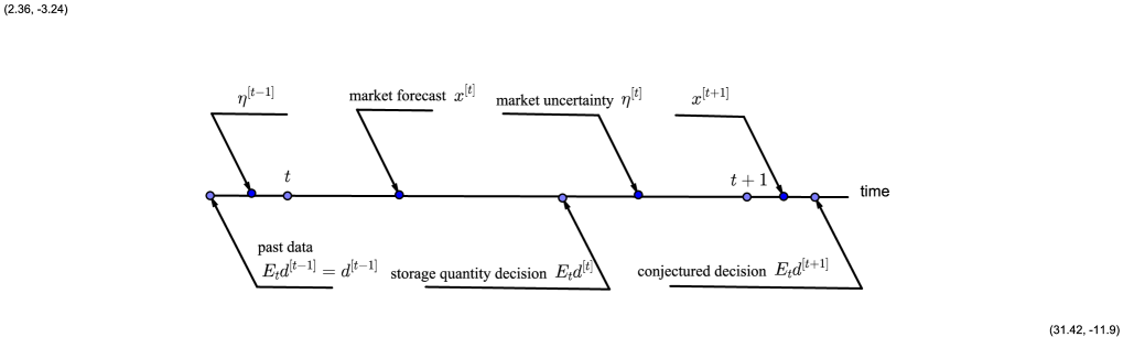
Figure 1: Timeline of the centralized storage model.

By the Principal of Optimality, in period $t$, we use the following induced sub-problem to find $\mathbb{E}_{t}d^{[t]}$ (optimal solution of $d^{[t]}$):

$$\max_{d^{[t]},d^{[t+1]},...,d^{[L]}}\sum_{\tau=t}^{\tau=L}\mathbb{E}\left[\left.\left(\beta^{[\tau]}-\gamma d^{[\tau]}+\eta^{[\tau]}\right)d^{[\tau]}-\varepsilon\cdot\left(d^{[\tau]}\right)^{2}\right|X^{[t]}\right],$$

subject to

$$\mathbb{E}\left[\left.\sum_{\tau=t}^{\tau=L}d^{[\tau]}\right|X^{[t]}\right]=-\sum_{\tau=1}^{\tau=t-1}d^{[\tau]}.$$ (5)

Proposition 1.

The optimal storage quantity in period $t$ is denoted by

$$\mathbb{E}_{t}d^{[t]} = \underset{\text{base storage quantity}}{\underbrace{\frac{\beta^{[t]}-\frac{\sum_{\tau=t}^{\tau=L}\beta^{[\tau]}}{L-t+1}}{2\left(\varepsilon+\gamma\right)}-\frac{\sum_{\tau=1}^{\tau=t-1}d^{[\tau]}}{L-t+1}}}$$ (7)

$$+\underset{\text{response factor}}{\underbrace{\frac{\left(1-\frac{\sum_{\tau=t}^{\tau=L}\delta^{\tau-t}}{L-t+1}\right)}{2\left(\varepsilon+\gamma\right)}}}\cdot\mathbb{E}\left[\left.\eta^{[t]}\right|X^{[t]}\right],$$

for $t=1,2,...,L-1$, wherein $\mathbb{E}\left[\left.\eta^{[t]}\right|X^{[t]}\right]=\frac{\rho}{\rho+\zeta}x^{[t]}+\frac{\zeta\delta}{\rho+\zeta}\eta^{[t-1]}$, for $t=2,...,L$, and $\mathbb{E}\left[\left.\eta^{[1]}\right|X^{[1]}\right]=\frac{\rho}{\rho+\alpha}x^{[1]}$. In the final period, $\mathbb{E}_{L}d^{[L]}=-\sum_{\tau=1}^{\tau=L-1}d^{[\tau]}$.

In this proposition, we are able to derive the optimal storage quantities in closed form, comprising of two parts: The first part is the base storage quantity, and the second part is the response factor multiplied by an estimation of the market price uncertainty. The base storage quantity decreases in $\varepsilon$ (cost coefficients with respect to the depth of discharge) and $\gamma$ ( energy price elasticity). The market price uncertainty is estimated by a convex combination of a current forecast and a last-period observation: $\mathbb{E}\left[\left.\eta^{[t]}\right|X^{[t]}\right]=\frac{\rho}{\rho+\zeta}x^{[t]}+\frac{\zeta\delta}{\rho+\zeta}\eta^{[t-1]}$. The weighting factors are proportional to their relative precision levels $\rho$ and $\zeta$. In additional, the last-period observation weights more when the intertemporal correlation is stronger ($\delta$ is higher).

From this proposition, we can clearly see that the optimal storage quantities depend on both variability (captured by market potential coefficient $\beta^{[t]}$) and uncertainty (captured by $\eta^{[t]}$) in market price. The base storage quantity demonstrates a downward distortion to the per-stage optimal storage quantity $\frac{\beta^{[t]}}{2\left(\varepsilon+\gamma\right)}$: The component $\frac{\sum_{\tau=t}^{\tau=L}\frac{\beta^{[\tau]}}{L-t+1}}{2\left(\varepsilon+\gamma\right)}$ is the average per-stage optimal storage quantity across all future periods, and the component $\frac{\sum_{\tau=1}^{\tau=t-1}d^{[\tau]}}{L-t+1}$ is subtracted to compensate the existing energy storage level built up in the past. The downward distortion ensures that the overall storage quantities offset each other, i.e., $\mathbb{E}\left[\left.\sum_{t\in T}d^{[t]}\right|X^{[t]}\right]=0$.

4.2 Decentralized Two-Period Model

In this section, we recover the superscript for $\gamma$ and $\varepsilon$. We also recover the subscript for $x_{i}^{[t]}$ since the storages observe heterogeneous information. To characterize the equilibrium outcome under such highly asymmetric information structure, we first introduce our solution concept.

Equilibrium concept. Storage $i$ chooses a storage quantity $d_{i}^{[1]}$ to maximize $\mathbb{E}[\pi_{i}|x_{i}^{[1]}]$, by forming an expectation of the other producers’ production levels $\mathbb{E}(d_{j}^{[1]}|x_{i}^{[1]})$, for $\forall j\neq i$. $d_{i}^{[2]}$ is determined thereafter, due to the constraint $d_{i}^{[1]}+d_{i}^{[2]}=0$, $\forall i\in I$. We focus exclusively on the linear symmetric Bayesian-Nash equilibrium, i.e., $d_{i}^{[1]}=A+Cx_{i}^{[1]},$ for some constants $A$ and $C$. We can interpret $A$ as the base storage quantity; $C$ as the response factors with respect to the forecast $x_{i}^{[1]}$, respectively.

Proposition 2.

For a two-period model under private market forecasting, the storage quantity in the linear symmetric Bayesian-Nash equilibrium is $d_{i}^{[1]}=A+Cx_{i}^{[1]}$ for every storage, wherein

$$A=\frac{\beta^{[1]}-\beta^{[2]}}{2\left(\varepsilon^{[1]}+\varepsilon^{[2]}\right)+(n+1)\left(\gamma^{[1]}+\gamma^{[2]}\right)},$$

$$C=\frac{(1-\delta)\rho}{\left[\begin{array}[]{c}(n-1)\left(\gamma^{[1]}+\gamma^{[2]}\right)\rho+\\ 2\left(\varepsilon^{[1]}+\varepsilon^{[2]}+\gamma^{[1]}+\gamma^{[2]}\right)(\alpha+\rho)\end{array}\right]}.$$

In period $t=1$, the base storage quantity $A$ is positive (selling energy) if and only if $\beta^{[1]}>\beta^{[2]}$, i.e., the energy price decreases at $t=2$. Conversely, the storage buys energy ($A<0$) when it can be sold at a higher price at $t=2$ ($\beta^{[1]}<\beta^{[2]}$). Consistent with our results in the single storage model, the base selling quantity decreases in $\sum_{t\in T}\varepsilon^{[t]}$ (cost coefficients with respect to the depth of discharge), and in $\sum_{t\in T}\gamma^{[t]}$ (aggregate energy price elasticity). Furthermore, when $A>0$, it decreases in the number of storages. This is because that the market competition is more intense as the number of Cournot competitors increases, and consequently, the price of energy decreases. The converse is true when $A<0$.

The reaction to private forecast $C$ is more aggressive when its precision $\rho$ increases, as a storage relies more on an accurate market forecast. The reactions to forecasts are less aggressive when the intertemporal correlation $\delta$ increases. In the extreme case where $\delta=1$, the storage does not respond to forecasts. Intuitively, this is because that any action (either buy or sell) in response to a market forecasts at $t=1$ will be offset by a reverse operation (under the energy balance constraints $\sum_{t\in T}d_{i}^{[t]}=0$) at $t=2$ when the market condition remains the same.

Proposition 3.

When there are a large number of storages, every storage’s equilibrium payoff converges asymptotically to

$$\lim_{n\rightarrow\infty}\mathbb{E}[\pi_{i}]\rightarrow\sum_{t=1,2}\left(\varepsilon^{[t]}+\gamma^{[t]}\right)\left[\begin{array}[]{c}\left(\frac{\beta^{[1]}-\beta^{[2]}}{\gamma^{[1]}+\gamma^{[2]}}\right)^{2}+\\ \left(\frac{1-\delta}{\gamma^{[1]}+\gamma^{[2]}}\right)^{2}\rho^{-1}\end{array}\right]\cdot n^{-2}.$$ (8)

When there are a large number of storages, $\lim_{n\rightarrow\infty}\mathbb{E}[\pi_{i}]$ decreases in $\rho$. This result demonstrates the negative economic value of a private forecast, and is interpreted as competition effect. Although storages’ private forecasts are independent, they lead to similar reaction to a market price shock. When the number of storages is large, the purchase or selling quantity responses are exaggerated and the over-precision in forecasts can lead to even lower payoffs. The inverse-square decay with respect to the number of storages demonstrates the impact of competition intensity.

We complement the analysis with the following numerical example, wherein $\beta^{[1]}-\beta^{[2]}=1$, $\varepsilon^{[1]}=\varepsilon^{[2]}=\gamma^{[1]}=\gamma^{[2]}=1$, and the payoff is calculated with a finite number of storages. We summarize the results in Figure 2. A storage’s payoff decreases in the autoregressive parameter $\delta$. As a storage’s reactions to forecasts are less responsive when the intertemporal correlation ($\delta$) increases, the economic value of market information also decreases. For a similar reason, a storage’s payoff also decreases in market uncertainty parameter $\alpha$, as the storage’s reactions to forecasts are also less responsive in this case. In addition, the inverse-square decay with respect to the number of storages confirms our result in the asymptotic analysis. Finally, a storage’s payoff first increases then decreases in its private information precision. When private information is scarce, the economic value of private information increases in its precision as it mitigate uncertainty. However, when the information precision further increases, the competition effect dominates and the payoff decreases.

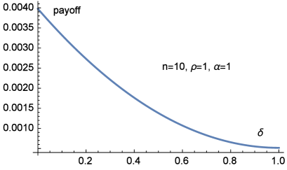
(a) Impact of autoregression parameter $\delta$.

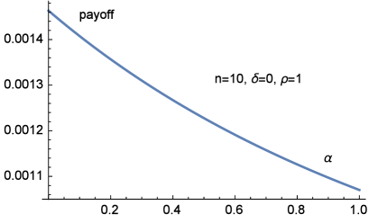
(b) Impact of market uncertainty parameter $\alpha$.

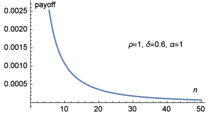
(c) Impact of the number of storages $n$.

(d) Impact of private information precision $\rho$.

Figure 2: Sensitivity analysis of individual storage’s payoff with respect to model primitives.

5 Operational Policy Analysis

5.1 Public Forecast Provision

Suppose that instead of private forecasts, all the storages receive a public forecast $x_{0}^{[t]}=\eta^{[t]}+\xi_{0}^{[t]}$, where $\xi_{0}^{[t]}\sim$ $N(0,\sigma^{-1})$. In this section, we analyze the possibility for a public forecast to coordinate storages’ actions. This can be potentially provided by the aggregator. Following a similar analysis as in the private forecasting model, we assume that $d_{i}^{[1]}=A+Bx_{0}^{[1]}$, where $B$ is the response factor towards the public forecast.

Proposition 4.

For a two-period model under public market forecasting, each storage’s equilibrium storage quantity in the linear symmetric Bayesian-Nash equilibrium is $d_{i}^{[1]}=A+Bx_{0}^{[1]}$, wherein

$$A=\frac{\beta^{[1]}-\beta^{[2]}}{2\left(\varepsilon^{[1]}+\varepsilon^{[2]}\right)+(n+1)\left(\gamma^{[1]}+\gamma^{[2]}\right)},$$

$$B=\frac{(1-\delta)\sigma/(\alpha+\sigma)}{2\left(\varepsilon^{[1]}+\varepsilon^{[2]}\right)+(n+1)\left(\gamma^{[1]}+\gamma^{[2]}\right)}.$$

The equilibrium payoff

$$\lim_{n\rightarrow\infty}\mathbb{E}[\pi_{i}]\rightarrow\sum_{t=1,2}\left(\varepsilon^{[t]}+\gamma^{[t]}\right)\left[\begin{array}[]{c}\left(\frac{\beta^{[1]}-\beta^{[2]}}{\gamma^{[1]}+\gamma^{[2]}}\right)^{2}\\ +\left(\frac{1-\delta}{\gamma^{[1]}+\gamma^{[2]}}\right)^{2}\cdot\frac{\sigma}{\left(\alpha+\sigma\right)^{2}}\end{array}\right]\cdot n^{-2}.$$

Similar to the private forecasting model, the reaction to public forecast $B$ is more aggressive when its precision $\sigma$ increases. $\lim_{n\rightarrow\infty}\mathbb{E}[\pi_{i}]$ is pseudo-concave in the public forecast precision $\sigma$, and thus reaches global maximum when $\sigma=\alpha$. Notice that, when $\sigma>\alpha$, $\lim_{n\rightarrow\infty}\mathbb{E}[\pi_{i}]$ decreases in $\sigma$, which demonstrate the negative economic value of a public forecast. We interpret this as congestion effect: Intuitively, when $\sigma>\alpha$, over-reaction to a public forecast leads to either too much purchase quantity (when forecast is favorable) or too much selling quantity (unfavorable forecast) from all storages. The public forecast becomes a herding signal. It is beneficial to maintain certain exclusiveness of a public forecast. For given information provision, a storage’s payoff suffers inverse-square decay in the number of storages, as the economic value of a public forecast is diluted when more storages respond to it.

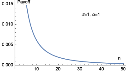
(a) Impact of number of storages $n$.

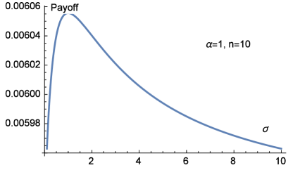
(b) Impact of public information precision $\sigma$.

Figure 3: Sensitivity analysis of individual storage’s payoff under public information provision.

We complement the analysis with the following numerical example summarized in Figure 3, wherein $\beta^{[1]}-\beta^{[2]}=1$, $\varepsilon^{[1]}=\varepsilon^{[2]}=\gamma^{[1]}=\gamma^{[2]}=1$, and the payoff is calculated with a finite number of storages. Again, a storage’s payoff decreases to the inverse-square of the number of storages as shown in the analytical result. A storage’s payoff first increases (due to positive economic value) then decreases (due to the congestion effect) in the precision of the public market forecast.

5.2 Encourage Information Sharing

Suppose that the storages pool their private forecasts $x_{i}^{[1]}$ together. In this case, it can be checked that it is equivalent for them to observe a public forecast $x_{0}^{[1]}$ with precision $\sigma=n\rho$:

$$\mathbb{E}[\eta^{[1]}|x_{1}^{[1]},...,x_{n}^{[1]}]=\frac{\rho}{\alpha+n\rho}\sum_{i\in I}x_{i}^{[1]},\mathbb{E}[\eta^{[1]}|x_{0}^{[1]}]=\frac{\sigma}{\alpha+\sigma}x_{0}^{[1]},$$

and it can be checked that these two estimators are stochastically equivalent, i.e., both $N(0,\frac{n\rho}{(\alpha+n\rho)^{2}})$.

Therefore, we can calculate the corresponding payoffs under pooling private forecasts:

$$\lim_{n\rightarrow\infty}\mathbb{E}[\pi_{i};\sigma = n\rho]\rightarrow\sum_{t=1,2}\left(\varepsilon^{[t]}+\gamma^{[t]}\right)\cdot\left[\begin{array}[]{c}\left(\frac{\beta^{[1]}-\beta^{[2]}}{\gamma^{[1]}+\gamma^{[2]}}\right)^{2}\\ +\left(\frac{1-\delta}{\gamma^{[1]}+\gamma^{[2]}}\right)^{2}\cdot\left(n\rho\right)^{-1}\end{array}\right]\cdot n^{-2}$$

$$< \sum_{t=1,2}\left(\varepsilon^{[t]}+\gamma^{[t]}\right)\left[\left(\frac{\beta^{[1]}-\beta^{[2]}}{\gamma^{[1]}+\gamma^{[2]}}\right)^{2}+\left(\frac{1-\delta}{\gamma^{[1]}+\gamma^{[2]}}\right)^{2}\rho^{-1}\right]\cdot n^{-2}.$$

By comparing this payoff with that under private forecasts, we find that the economic value of forecast under information sharing is (to an order of magnitude in the number of storages) lower than that under private forecasts. There will be no incentive for the storage to share information with each others. From this analysis, we find that communication among the storages fails to achieve a coordinated effort to increase market efficiency. To maintain the exclusiveness of their private forecasts, the decentralized storages should not be encouraged to share market information in this regime. This result is confirmed by a numerical analysis summarized in Figure 4 when there are a large number of storages. However, when the number of storages is small, it is possible that every storage is better off by information sharing. This regime is possible when each private forecast is extremely fuzzy, and pooling them together can amplify the market signal.

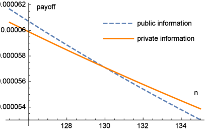
(a) Small number of energy storages.

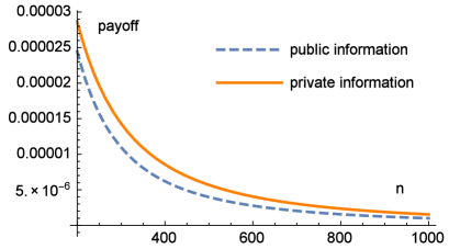
(b) Large number of energy storages.

Figure 4: Individual payoff comparison with and without information sharing.

5.3 Targeted Information Release

Now that we know the exclusiveness of a market forecast is important, we analyze an alternative policy intervention through public information channel. Suppose that the aggregator/government offers a public forecast only to a subset of storages $J$ ($|J|=m\leq n$). For informed storages (ones who receive the public forecast), their $d_{i}^{[1]}=A+Bx_{0}^{[1]}$, $\forall i$ $\in J$. For uninformed storages, their $d_{i}^{[1]}=C$, $\forall i$ $\in I-J$. $A$, $B$ and $C$ are all unknown constant coefficients.

Proposition 5.

For a two-period model under targeted information release, storages’ equilibrium storage quantities in the linear Bayesian-Nash equilibrium are $d_{i}^{[1]}=A+Bx_{0}^{[1]}$, $\forall i$ $\in J$, and $d_{i}^{[1]}=C$, $\forall i$ $\in I-J$, wherein

$$A=C=\frac{\beta^{[1]}-\beta^{[2]}}{2\left(\varepsilon^{[1]}+\varepsilon^{[2]}\right)+(n+1)\left(\gamma^{[1]}+\gamma^{[2]}\right)},$$

$$B=\frac{(1-\delta)\sigma/(\alpha+\sigma)}{2\left(\varepsilon^{[1]}+\varepsilon^{[2]}\right)+(m+1)\left(\gamma^{[1]}+\gamma^{[2]}\right)}.$$

The storages’ aggregate payoff $\sum_{i\in I}\mathbb{E}[\pi_{i}]$ is maximized when the population of information recipient

$$m=1+\frac{2\left(\varepsilon^{[1]}+\varepsilon^{[2]}\right)}{\gamma^{[1]}+\gamma^{[2]}}.$$ (10)

In this case, the storages’ payoffs are stratified, due to their asymmetrical informational status. The fact that an interior solution (of $m$) exists suggests a trade-off between the economic value of a public forecast in coordinating the storages’ actions, and the congestion effect due to the lack of exclusiveness of such information dissemination.

6 Model Generalizations

6.1 Multi-Period Model

In this section, we demonstrate that the model can be extended in multiple directions. A multi-period version of this problem has to be solved recursively using backward induction while unfolding the information set throughout the process. Instead, we analyze a relaxed problem. In this case, equilibrium characterization requires solving the following optimization problems:

$$\max_{d_{i}^{[t]},t\in T}\sum_{t\in T}\mathbb{E}\left[\left.\begin{array}[]{c}P^{[t]}(D^{[t]})\cdot d_{i}^{[t]}\\ -\varepsilon^{[t]}\cdot\left(d_{i}^{[t]}\right)^{2}\end{array}\right|X_{i}^{[t]}\right],$$

subject to

$$\mathbb{E}\left[\sum_{t\in T}d_{i}^{[t]}\right]=0.$$ (11)

$X_{i}^{[t]}=\left\{x_{0}^{[1]},x_{i}^{[1]},\eta^{[1]},...,\eta^{[t-1]},x_{0}^{[t]},x_{i}^{[t]}\right\}$ indicates the corresponding information set. Notice that we simultaneous incorporate private forecasts $\{x_{i}^{[t]}\}$’s and a public forecast $x_{0}^{[t]}$. The storage quantity will be $d_{i}^{[t]}=A^{[t]}+B^{[t]}x_{0}^{[t]}+C^{[t]}x_{i}^{[t]}$ for some unknown coefficients $A^{[t]}$, $B^{[t]}$ and $C^{[t]}$. This is a relaxation because an exact solution requires that $\mathbb{E}\left[\left.\sum_{t\in T}\left(d_{i}^{[t]}\right)^{\ast}\right|X_{i}^{[t]}\right]=0$, for any sample path generated by $\{X_{i}^{[t]}\}^{\prime}s$.

Proposition 6.

For a multi-period model under both private and public market forecasting, the storage quantities in the linear symmetric Bayesian-Nash equilibrium can be approximated by $d_{i}^{[t]}=A^{[t]}+B^{[t]}x_{0}^{[t]}+C^{[t]}x_{i}^{[t]}$, wherein

$$A^{[t]}=\frac{\beta^{[t]}-\lambda}{2\varepsilon^{[t]}+(n+1)\gamma^{[t]}},$$

$$C^{[t]}=\frac{\rho}{\left[2\left(\varepsilon^{[t]}+\gamma^{[t]}\right)(\alpha+\sigma+\rho)+(n-1)\gamma^{[t]}\rho\right]},$$

$$B^{[t]}=\frac{\sigma-(n-1)\gamma^{[t]}\sigma C}{\left[(n+1)\gamma^{[t]}+2\varepsilon^{[t]}\right](\alpha+\sigma+\rho)},$$

and the Lagrangian multiplier

$$\lambda=\frac{\sum_{t\in T}\beta^{[t]}\prod\limits_{\tau\neq t}\left[2\varepsilon^{[\tau]}+(n+1)\gamma^{[\tau]}\right]}{\sum_{t\in T}\prod\limits_{\tau\neq t}\left[2\varepsilon^{[\tau]}+(n+1)\gamma^{[\tau]}\right]}.$$ (12)

.

The downside of this analysis is that we can not guarantee that $\mathbb{E}\left[\left.\sum_{t\in T}\left(d_{i}^{[t]}\right)^{\ast}\right|X_{i}^{[t]}\right]=0$. Essentially, the storages reduce the baseline quantity $A^{[t]}$ by their time-average so that the aggregate buy/sell quantities sum up to zero in the statistical sense. This approximation of the storages’ actions ignores the intertemporal correlation of uncertainties. Future research is needed for an exact analysis of the full-fledged model.

6.2 Heterogeneous Storages

We model storages with heterogeneous physical attributes and information status by assuming that the costs of utilizing storage $c_{i}(d)=\varepsilon_{i}^{[t]}\cdot d^{2}$, and storage $i$ receives a private forecast $x_{i}^{[t]}$ with precision $\rho_{i}$. To illustrate the major points, we extend the two-period model.

Proposition 7.

For a two-period model under both private and public market forecasting, the heterogeneous storage quantities in the linear Bayesian-Nash equilibrium take the form of $d_{i}^{[1]}=A_{i}+B_{i}x_{0}^{[1]}+C_{i}x_{i}^{[1]}$, wherein $A_{i}$, $B_{i}$, and $C_{i}$ are given in the Appendix.

As in the basic model with homogeneous storages, each storage holds their own forecast but with varying precision:

$$\mathbb{E}[\eta^{[1]}|x_{0}^{[1]},x_{i}^{[1]}]=\frac{\sigma}{\alpha+\sigma+\rho}x_{0}^{[1]}+\frac{\rho_{i}}{\alpha+\sigma+\rho_{i}}x_{i}^{[1]}.$$ (13)

The interesting new feature in this extension is that each storage ($i$) needs to guess another storage’s ($j$) quantity decision via its own information set:

$$\mathbb{E}[d_{j}^{[1]}|x_{0}^{[1]},x_{i}^{[1]}]=A_{j}+B_{j}x_{0}^{[1]}+C_{j}\mathbb{E}[x_{j}^{[1]}|x_{0}^{[1]},x_{i}^{[1]}].$$ (14)

To obtain a correct conjecture, storage $i$ needs to estimate storage $j$’s private forecast:

$$\mathbb{E}[x_{j}^{[1]}|x_{0}^{[1]},x_{i}^{[1]}]=\mathbb{E}[\eta^{[1]}+\xi_{j}^{[1]}|x_{0}^{[1]},x_{i}^{[1]}]=\mathbb{E}[\eta^{[1]}|x_{0}^{[1]},x_{i}^{[1]}].$$ (15)

Following a similar procedure as in the basic homogeneous model, we can obtain the coefficients summarized in the Appendix. The dependency of the value of both public and private forecasts on their precisions $\sigma$ and $\rho_{i}$ is highly nonlinear. Due to the complicated payoff functional forms of this general model, we start with the homogeneous model for a clear presentation of results. It can be checked that some of our findings and intuitions remain robust under this generalization. For example, the base storage quantity $A$ is positive (selling energy) if and only if $\beta^{[1]}>\beta^{[2]}$, i.e., the energy price decreases at $t=2$. The value of a private forecast ($C_{i}^{2}\mathbb{E}[x_{i}^{[1]}]^{2}$) is proportional to $\left[\frac{(1-\delta)}{\alpha+\sigma+\rho_{i}}\right]^{2}\rho_{i}$, and thus decreasing in the intertemporal correlation $\delta$, as the reactions to forecasts are less aggressive when $\delta$ increases.

7 Conclusion

In this paper, we propose stylized models of decentralized energy storage planning under private and public market forecasting, when energy prices are both uncertain and variable over time. We derive the optimal buying or selling quantities for storages in a competitive environment with strategic interactions. Coarsely speaking, a foresighted storage will plan to buy energy when its price is low and sell when the price high. The value of a private forecast decreases in the intertemporal correlation of market price shock. We demonstrate the potentially negative economic value of a private forecast, due to competition effect: When there are a large number of storages, the purchase or selling quantity responses are exaggerated and the over-precision in forecasts can lead to even lower payoffs. These fundamental observations are robust when we generalize the model to multi-period or heterogeneous storages.

We also examine several information management policies to coordinate storages’ actions and improve their profitability. Firstly, we demonstrate the potential negative economic value of a public forecast, due to congestion effect: A precise public forecast leads to herding behavior, and over-reaction to a public forecast leads to either too much purchase quantity (when forecast is favorable) or too much selling quantity (unfavorable forecast) from all storages. Secondly, we find that communication among the storages could fail to achieve a coordinated effort to increase market efficiency. The decentralized storages will not participate in any information sharing program when there are a large number of storages. Thirdly, we find it optimal to release additional information to a subset of energy storages exclusively by targeted information release.

Future research is needed for a full-fledged analysis of a multi-period, decentralized, and heterogeneous model. Another direction to go is to incorporate operational constraints such as energy and/or power limits. Explicit modeling of renewable energy generation will contribute to a holistic understanding of the entire integrated system. Finally, information management research in other energy markets is likely to be promising.

Appendix A Appendix. Proofs.

Proof of Proposition 1. Introduce a Lagrangian multiplier $\lambda^{[t]}$ to relax the conservation constraint. We denote the Lagrangian by

$$L = \sum_{\tau=t}^{\tau=L}l^{[\tau]}$$ (18)

$$= \sum_{\tau=t}^{\tau=L}\mathbb{E}\left[\left.\begin{array}[]{c}\left(\beta^{[\tau]}-\gamma d^{[\tau]}+\eta^{[\tau]}\right)d^{[\tau]}\\ -\varepsilon\cdot\left(d^{[\tau]}\right)^{2}-\lambda^{[t]}d^{[\tau]}\end{array}\right|X^{[t]}\right]-\lambda^{[t]}\sum_{\tau=1}^{\tau=t-1}d^{[\tau]}$$

By the first-order condition $\frac{\partial l^{[\tau]}}{\partial d^{[\tau]}}=0$, for $\tau=t,...,L$ $\Rightarrow$

$$\mathbb{E}_{t}d^{[\tau]}=\frac{\beta^{[\tau]}-\lambda^{[t]}+\mathbb{E}\left[\left.\eta^{[\tau]}\right|X^{[t]}\right]}{2\left(\varepsilon+\gamma\right)}.$$ (19)

Notice that $\mathbb{E}\left[\left.\eta^{[\tau]}\right|X^{[t]}\right]=\delta^{\tau-t}\mathbb{E}\left[\left.\eta^{[t]}\right|X^{[t]}\right]$, for $\tau=t,...,L$, and $\mathbb{E}\left[\left.\sum_{\tau=t}^{\tau=L}d^{[\tau]}\right|X^{[t]}\right]=-\sum_{\tau=1}^{\tau=t-1}d^{[\tau]}\Rightarrow$

$$\lambda^{[t]}=\frac{\sum_{\tau=t}^{\tau=L}\beta^{[\tau]}+\sum_{\tau=t}^{\tau=L}\delta^{\tau-t}\mathbb{E}\left[\left.\eta^{[t]}\right|X^{[t]}\right]+2\left(\varepsilon+\gamma\right)\sum_{\tau=1}^{\tau=t-1}d^{[\tau]}}{L-t+1}$$ (20)

Therefore,

$$\mathbb{E}_{t}d^{[t]}=\frac{\beta^{[t]}-\frac{\sum_{\tau=t}^{\tau=L}\beta^{[\tau]}}{L-t+1}}{2\left(\varepsilon+\gamma\right)}+\frac{\left(1-\frac{\sum_{\tau=t}^{\tau=L}\delta^{\tau-t}}{L-t+1}\right)\mathbb{E}\left[\left.\eta^{[t]}\right|X^{[t]}\right]}{2\left(\varepsilon+\gamma\right)}-\frac{\sum_{\tau=1}^{\tau=t-1}d^{[\tau]}}{L-t+1}.$$ (21)

$\square$

Proof of Proposition 2. The payoff can be simplified by plugging $d_{i}^{[2]}=-d_{i}^{[1]}.$ To derive the equilibrium storage quantities, we set $\frac{\partial\mathbb{E}[\pi_{i}|x_{i}^{[1]}]}{\partial d_{i}^{[1]}}=0$:

$$\left[\begin{array}[]{c}\beta^{[1]}-\beta^{[2]}-\left(\gamma^{[1]}+\gamma^{[2]}\right)\sum_{j\neq i}\mathbb{E}[d_{j}^{[1]}|x_{i}^{[1]}]\\ +\mathbb{E}[\eta^{[1]}|x_{i}^{[1]}]-\mathbb{E}[\eta^{[2]}|x_{i}^{[1]}]\\ -2\left(\gamma^{[1]}+\gamma^{[2]}+\varepsilon^{[1]}+\varepsilon^{[2]}\right)\cdot d_{i}^{[1]}\end{array}\right]=0.$$ (22)

Notice that

$$\mathbb{E}[d_{j}^{[1]}|x_{i}^{[1]}]=A+Bx_{0}^{[1]}+C\mathbb{E}[x_{j}^{[1]}|,x_{i}^{[1]}],$$

$$\mathbb{E}[x_{j}^{[1]}|x_{i}^{[1]}] = \mathbb{E}[\eta^{[1]}+\xi_{j}^{[1]}|x_{i}^{[1]}]$$

$$= \mathbb{E}[\eta^{[1]}|x_{i}^{[1]}],$$

$$\mathbb{E}[\eta^{[2]}|x_{i}^{[1]}] = \mathbb{E}[\delta\eta^{[1]}+\epsilon_{1}|x_{i}^{[1]}]$$

$$= \delta\mathbb{E}[\eta^{[1]}|x_{i}^{[1]}],$$

$$\mathbb{E}[\eta^{[1]}|x_{i}^{[1]}]=\frac{\rho}{\alpha+\rho}x_{i}^{[1]}.$$

By matching the coefficients with respect to $x_{i}^{[1]}$, we have

$$A=\frac{\beta^{[1]}-\beta^{[2]}}{2\left(\varepsilon^{[1]}+\varepsilon^{[2]}\right)+(n+1)\left(\gamma^{[1]}+\gamma^{[2]}\right)},$$

$$C=\frac{(1-\delta)\rho}{\left[\begin{array}[]{c}(n-1)\left(\gamma^{[1]}+\gamma^{[2]}\right)\rho+\\ 2\left(\varepsilon^{[1]}+\varepsilon^{[2]}+\gamma^{[1]}+\gamma^{[2]}\right)(\alpha+\rho)\end{array}\right]}.$$

$\square$

Proof of Proposition 3. The payoff can be calculated through

$$\mathbb{E}[\pi_{i}] = \mathbb{E}\left[\mathbb{E}[\pi_{i}|x_{i}^{[1]}]\right]$$ (23)

$$= \left(\varepsilon^{[1]}+\varepsilon^{[2]}+\gamma^{[1]}+\gamma^{[2]}\right)$$

$$\cdot\left(A^{2}+C^{2}\mathbb{E}[x_{i}^{[1]}]^{2}\right).$$

Notice that storage $i$’s payoff $\mathbb{E}[\pi_{i}]=\sum_{t\in T}\left(\varepsilon^{[t]}+\gamma^{[t]}\right)A^{2}$ when there is no information available. The additional payoff proportional to $C^{2}\mathbb{E}[x_{i}^{[1]}]^{2}$ corresponds to the economic value of the private forecast.

$$\lim_{n\rightarrow\infty}\mathbb{E}[\pi_{i}] = \lim_{n\rightarrow\infty}\sum_{t=1,2}\left(\varepsilon^{[t]}+\gamma^{[t]}\right)\left[\begin{array}[]{c}\frac{\left(\beta^{[1]}-\beta^{[2]}\right)^{2}}{(n+1)^{2}\left(\gamma^{[1]}+\gamma^{[2]}\right)2}\\ +\frac{(1-\delta)^{2}}{(n-1)^{2}\left(\gamma^{[1]}+\gamma^{[2]}\right)^{2}\rho}\end{array}\right]$$ (29)

$$\lim_{n\rightarrow\infty}\sum_{t=1,2}\left(\varepsilon^{[t]}+\gamma^{[t]}\right)\left[\begin{array}[]{c}\left(\frac{\beta^{[1]}-\beta^{[2]}}{\gamma^{[1]}+\gamma^{[2]}}\right)^{2}+\\ \left(\frac{1-\delta}{\gamma^{[1]}+\gamma^{[2]}}\right)^{2}\rho^{-1}\end{array}\right]\cdot n^{-2}.$$

$\square$

Proof of Proposition 4. To derive the equilibrium storage quantities, we set $\frac{\partial\mathbb{E}[\pi_{i}|x_{0}^{[1]}]}{\partial d_{i}^{[1]}}=0$:

$$\left[\begin{array}[]{c}\beta^{[1]}-\beta^{[2]}-\left(\gamma^{[1]}+\gamma^{[2]}\right)\sum_{j\neq i}\mathbb{E}[d_{j}^{[1]}|x_{0}^{[1]}]\\ +\mathbb{E}[\eta^{[1]}|x_{0}^{[1]}]-\mathbb{E}[\eta^{[2]}|x_{0}^{[1]}]\\ -2\left(\gamma^{[1]}+\gamma^{[2]}+\varepsilon^{[1]}+\varepsilon^{[2]}\right)\cdot d_{i}^{[1]}\end{array}\right]=0.$$ (30)

Notice that $\mathbb{E}[d_{j}^{[1]}|x_{0}^{[1]}]=A+Bx_{0}^{[1]},$ since $x_{0}^{[1]}$ is common knowledge. $\mathbb{E}[\eta^{[1]}|x_{0}^{[1]}]=\frac{\sigma}{\alpha+\sigma}x_{0}^{[1]}$, and

$$\mathbb{E}[\eta^{[2]}|x_{0}^{[1]}] = \mathbb{E}[\delta\eta^{[1]}+\epsilon_{1}|x_{0}^{[1]}]$$

$$= \delta\mathbb{E}[\eta^{[1]}|x_{0}^{[1]}].$$

By matching the coefficients with respect to $x_{i}^{[1]}$, we have

$$A=\frac{\beta^{[1]}-\beta^{[2]}}{2\left(\varepsilon^{[1]}+\varepsilon^{[2]}\right)+(n+1)\left(\gamma^{[1]}+\gamma^{[2]}\right)},$$

$$B=\frac{(1-\delta)\sigma/(\alpha+\sigma)}{\left[\begin{array}[]{c}2\left(\varepsilon^{[1]}+\varepsilon^{[2]}+\gamma^{[1]}+\gamma^{[2]}\right)\\ +\left(\gamma^{[1]}+\gamma^{[2]}\right)(n-1)\end{array}\right]}.$$

The corresponding payoff can be calculated as follows:

$$\mathbb{E}[\pi_{i}]=\sum_{t=1,2}\left(\varepsilon^{[t]}+\gamma^{[t]}\right)$$

$$\cdot\left\{\begin{array}[]{c}\left[\frac{\beta^{[1]}-\beta^{[2]}}{\sum_{t=1,2}2\left(\varepsilon^{[t]}+\gamma^{[t]}\right)+(n-1)\left(\gamma^{[1]}+\gamma^{[2]}\right)}\right]^{2}\\ +\left[\frac{(1-\delta)}{\sum_{t=1,2}2\left(\varepsilon^{[t]}+\gamma^{[t]}\right)+\left(\gamma^{[1]}+\gamma^{[2]}\right)(n-1)}\right]^{2}\cdot\frac{\sigma}{\left(\alpha+\sigma\right)^{2}}\end{array}\right\}.$$ (31)

$$\lim_{n\rightarrow\infty}\mathbb{E}[\pi_{i}]\rightarrow\sum_{t=1,2}\left(\varepsilon^{[t]}+\gamma^{[t]}\right)\left[\begin{array}[]{c}\left(\frac{\beta^{[1]}-\beta^{[2]}}{\gamma^{[1]}+\gamma^{[2]}}\right)^{2}\\ +\left(\frac{1-\delta}{\gamma^{[1]}+\gamma^{[2]}}\right)^{2}\cdot\frac{\sigma}{\left(\alpha+\sigma\right)^{2}}\end{array}\right]\cdot n^{-2}.$$

$\square$

Proof of Proposition 5. To solve for equilibrium storage quantities, we set $\frac{\partial\mathbb{E}[\pi_{i}|x_{0}^{[1]}]}{\partial d_{i}^{[1]}}=0$ for $\forall i$ $\in J$ and $\frac{\partial\pi_{i}}{\partial d_{i}^{[1]}}=0$ for $\forall i$ $\in I-J$, separately. For $\forall i\in J,$

$$\begin{array}[]{c}\beta^{[1]}-\beta^{[2]}-\left(\gamma^{[1]}+\gamma^{[2]}\right)\left[\begin{array}[]{c}(n-m)C+\\ (m-1)\left(A+Bx_{0}^{[1]}\right)\end{array}\right]\\ +\frac{(1-\delta)\sigma}{\alpha+\sigma}x_{0}^{[1]}-2\left(\begin{array}[]{c}\gamma^{[1]}+\gamma^{[2]}\\ +\varepsilon^{[1]}+\varepsilon^{[2]}\end{array}\right)\cdot\left(A+Bx_{0}^{[1]}\right)\end{array}=0,$$ (32)

whereas for $\forall i\in I-J,$

$$\begin{array}[]{c}\beta^{[1]}-\beta^{[2]}-\left(\gamma^{[1]}+\gamma^{[2]}\right)\left[\begin{array}[]{c}mA+\\ (n-m-1)C\end{array}\right]\\ -2\left(\begin{array}[]{c}\gamma^{[1]}+\gamma^{[2]}\\ +\varepsilon^{[1]}+\varepsilon^{[2]}\end{array}\right)\cdot C\end{array}=0.$$ (33)

Matching coefficients with respect to $x_{0}^{[1]}$, we can obtain $A,B$ and $C$ following a similar procedure as before. We measure the economic efficiency by aggregate payoff:

$$\sum_{i\in I}\mathbb{E}[\pi_{i}]=\left(\varepsilon^{[1]}+\varepsilon^{[2]}+\gamma^{[1]}+\gamma^{[2]}\right)$$

$$\cdot\left(nA^{2}+\frac{(1-\delta)^{2}m}{\left[\begin{array}[]{c}2\left(\gamma^{[1]}+\gamma^{[2]}+\varepsilon^{[1]}+\varepsilon^{[2]}\right)\\ +(m-1)\left(\gamma^{[1]}+\gamma^{[2]}\right)\end{array}\right]^{2}}\frac{\sigma}{\left(\alpha+\sigma\right)^{2}}\right).$$ (34)

It can be checked that the storages’ aggregate payoff $\sum_{i\in I}\mathbb{E}[\pi_{i}]$ is maximized when

$$m=1+\frac{2\left(\varepsilon^{[1]}+\varepsilon^{[2]}\right)}{\gamma^{[1]}+\gamma^{[2]}}.$$ (35)

$\square$

Proof of Proposition 6. The payoff from storage $i$ under a Lagrangian relaxation can be expressed as

$$L_{i}\left(d_{i}^{[t]},t\in T\right)=\sum_{t\in T}l_{i}^{[t]}\left(d_{i}^{[t]}\right)$$

$$= \sum_{t\in T}\mathbb{E}\left[\left.\begin{array}[]{c}P^{[t]}(D^{[t]})\cdot d_{i}^{[t]}\\ -\varepsilon^{[t]}\cdot\left(d_{i}^{[t]}\right)^{2}\end{array}\right|X_{i}^{[t]}\right]-\lambda^{[t]}\mathbb{E}\left[\left.\sum_{t\in T}d_{i}^{[t]}\right|X_{i}^{[t]}\right]$$ (38)

$$= \sum_{t\in T}\mathbb{E}\left[\left.\begin{array}[]{c}P^{[t]}(D^{[t]})\cdot d_{i}^{[t]}\\ -\varepsilon^{[t]}\cdot\left(d_{i}^{[t]}\right)^{2}-\lambda^{[t]}d_{i}^{[t]}\end{array}\right|X_{i}^{[t]}\right],$$ (41)

wherein $\lambda^{[t]}$ is a Lagrangian multiplier to relax the constraint that $\mathbb{E}\left[\left.\sum_{t\in T}d_{i}^{[t]}\right|X_{i}^{[t]}\right]=0$. To solve for equilibrium storage quantities, we set $\frac{\partial l_{i}^{[t]}\left(d_{i}^{[t]}\right)}{\partial d_{i}^{[t]}}=0$:

$$\left[\begin{array}[]{c}\beta^{[t]}-\gamma^{[t]}\sum_{j\neq i}\mathbb{E}[d_{j}^{[t]}|X_{i}^{[t]}]\\ +\mathbb{E}[\eta^{[t]}|X_{i}^{[t]}]-2\left(\gamma^{[t]}+\varepsilon^{[t]}\right)\cdot d_{i}^{[1]}-\lambda^{[t]}\end{array}\right]=0.$$ (42)

By $\mathbb{E}\left[\sum_{t\in T}\left(d_{i}^{[t]}\right)^{\ast}\right]=0$, we use $\lambda$ as a static approximate solution instead of $\lambda^{[t]}$. $\square$

Proof of Proposition 7. Again, the first-order condition for payoff-maximization requires

$$\left[\begin{array}[]{c}\beta^{[1]}-\beta^{[2]}-\left(\gamma^{[1]}+\gamma^{[2]}\right)\sum_{j\neq i}\mathbb{E}[d_{j}^{[1]}|x_{0}^{[1]},x_{i}^{[1]}]\\ +\mathbb{E}[\eta^{[1]}|x_{0}^{[1]},x_{i}^{[1]}]-\mathbb{E}[\eta^{[2]}|x_{0}^{[1]},x_{i}^{[1]}]\\ -2\left(\gamma^{[1]}+\gamma^{[2]}+\varepsilon_{i}^{[1]}+\varepsilon_{i}^{[2]}\right)\cdot d_{i}^{[1]}\end{array}\right]=0.$$ (43)

The unknown coefficients in the equilibrium buying or selling quantities are summarized as follows.

$$A_{i} = \frac{\beta^{[1]}-\beta^{[2]}}{2\left(\varepsilon_{i}^{[1]}+\varepsilon_{i}^{[2]}\right)+\left(\gamma^{[1]}+\gamma^{[2]}\right)}$$ (44)

$$\cdot\left[\sum_{i\in I}\frac{\left(\gamma^{[1]}+\gamma^{[2]}\right)}{2\left(\varepsilon_{i}^{[1]}+\varepsilon_{i}^{[2]}\right)+\left(\gamma^{[1]}+\gamma^{[2]}\right)}+1\right]^{-1}.$$

$$C_{i} = -\frac{\left(\gamma^{[1]}+\gamma^{[2]}\right)\frac{(1-\delta)\rho_{i}}{\alpha+\sigma+\rho_{i}}}{\left[2\left(\begin{array}[]{c}\gamma^{[1]}+\gamma^{[2]}\\ +\varepsilon_{i}^{[1]}+\varepsilon_{i}^{[2]}\end{array}\right)-\left(\gamma^{[1]}+\gamma^{[2]}\right)\frac{\rho_{i}}{\alpha+\sigma+\rho_{i}}\right]}$$ (50)

$$\cdot\frac{\sum_{i\in I}\frac{\frac{\rho_{i}}{\alpha+\sigma+\rho_{i}}}{\left[2\left(\gamma^{[1]}+\gamma^{[2]}+\varepsilon_{i}^{[1]}+\varepsilon_{i}^{[2]}\right)-\left(\gamma^{[1]}+\gamma^{[2]}\right)\frac{\rho_{i}}{\alpha+\sigma+\rho_{i}}\right]}}{1+\sum_{i\in I}\frac{\left(\gamma^{[1]}+\gamma^{[2]}\right)\frac{\rho_{i}}{\alpha+\sigma+\rho_{i}}}{\left[2\left(\gamma^{[1]}+\gamma^{[2]}+\varepsilon_{i}^{[1]}+\varepsilon_{i}^{[2]}\right)-\left(\gamma^{[1]}+\gamma^{[2]}\right)\frac{\rho_{i}}{\alpha+\sigma+\rho_{i}}\right]}}$$

$$+\frac{\frac{(1-\delta)\rho_{i}}{\alpha+\sigma+\rho_{i}}}{\left[2\left(\begin{array}[]{c}\gamma^{[1]}+\gamma^{[2]}\\ +\varepsilon_{i}^{[1]}+\varepsilon_{i}^{[2]}\end{array}\right)-\left(\gamma^{[1]}+\gamma^{[2]}\right)\frac{\rho_{i}}{\alpha+\sigma+\rho_{i}}\right]}.$$

$$B_{i} = -\frac{\left(\gamma^{[1]}+\gamma^{[2]}\right)\left(\sum_{i\in I}B_{i}+\frac{\sigma}{\alpha+\sigma+\rho_{i}}\sum_{j\neq i}C_{j}\right)}{\left[2\left(\varepsilon_{i}^{[1]}+\varepsilon_{i}^{[2]}\right)+\left(\gamma^{[1]}+\gamma^{[2]}\right)\right]}$$ (51)

$$+\frac{\frac{(1-\delta)\sigma}{\alpha+\sigma+\rho_{i}}}{\left[2\left(\varepsilon_{i}^{[1]}+\varepsilon_{i}^{[2]}\right)+\left(\gamma^{[1]}+\gamma^{[2]}\right)\right]},$$

wherein

$$\sum_{i\in I}B_{i} = -\frac{\sum_{i\in I}\frac{\left(\gamma_{i}^{[1]}+\gamma_{i}^{[2]}\right)\frac{\sigma}{\alpha+\sigma+\rho_{i}}\sum_{j\neq i}C_{j}}{2\left(\varepsilon_{i}^{[1]}+\varepsilon_{i}^{[2]}\right)+\left(\gamma_{i}^{[1]}+\gamma_{i}^{[2]}\right)}}{\left[1+\sum_{i\in I}\frac{\left(\gamma_{i}^{[1]}+\gamma_{i}^{[2]}\right)}{2\left(\varepsilon_{i}^{[1]}+\varepsilon_{i}^{[2]}\right)+\left(\gamma_{i}^{[1]}+\gamma_{i}^{[2]}\right)}\right]}$$ (52)

$$+\frac{\sum_{i\in I}\frac{\frac{(1-\delta)\sigma}{\alpha+\sigma+\rho_{i}}}{2\left(\varepsilon_{i}^{[1]}+\varepsilon_{i}^{[2]}\right)+\left(\gamma^{[1]}+\gamma^{[2]}\right)}}{\left[1+\sum_{i\in I}\frac{\left(\gamma^{[1]}+\gamma^{[2]}\right)}{2\left(\varepsilon_{i}^{[1]}+\varepsilon_{i}^{[2]}\right)+\left(\gamma^{[1]}+\gamma^{[2]}\right)}\right]}.$$

$\square$

References

- Acemoglu et al. (2015) Acemoglu, D., A. Kakhbod, and A. Ozdaglar (2015). Competition in electricity markets with renewable energy sources. Technical report, Massachusetts Institute of Technology.
- Borenstein and Bushnell (1999) Borenstein, S. and J. Bushnell (1999). An empirical analysis of the potential for market power in California electricity industry. The Journal of Industrial Economics 47(3), 285–323.
- Contreras-Ocana et al. (2015) Contreras-Ocana, J. E., M. A. Ortega-Vazquez, and B. Zhang (2015). Cooperation and competition among energy storages. arXiv preprint arXiv:1511.02201.
- Dicorato et al. (2012) Dicorato, M., G. Forte, M. Pisani, and M. Trovato (2012). Planning and operating combined wind-storage system in electricity market. IEEE Transactions on Sustainable Energy 3(2), 209–217.
- Gal-Or (1985) Gal-Or, E. (1985). Information sharing in oligopoly. Econometrica: Journal of the Econometric Society, 329–343.
- Grothoff (2015) Grothoff, J. M. (2015). Battery storage for renewables: Market status and technology outlook. Technical report, International Renewable Energy Agency (IRENA).
- Haessig et al. (2015) Haessig, P., B. Multon, H. B. Ahmed, S. Lascaud, and P. Bondon (2015). Energy storage sizing for wind power: Impact of the autocorrelation of day-ahead forecast errors. Wind Energy 18(1), 43–57.
- Kamalinia et al. (2014) Kamalinia, S., M. Shahidehpour, and L. Wu (2014). Sustainable resource planning in energy markets. Applied Energy 133, 112–120.
- Langary et al. (2014) Langary, D., N. Sadati, and A. M. Ranjbar (2014). Direct approach in computing robust Nash strategies for generating companies in electricity markets. International Journal of Electrical Power & Energy Systems 54, 442–453.
- Li et al. (2016) Li, C.-T., H. Peng, and J. Sun (2016). Predictive control and sizing of energy storage to mitigate wind power intermittency. Wind Energy 19(3), 437–451.
- Li and Shahidehpour (2005) Li, T. and M. Shahidehpour (2005). Strategic bidding of transmission-constrained GENCOs with incomplete information. IEEE Transactions on Power Systems 20(1), 437–447.
- Morris and Shin (2002) Morris, S. and H. S. Shin (2002). Social value of public information. The American Economic Review 92(5), 1521–1534.
- Motors (2016) Motors, T. (2016). Tesla power wall. URL https://www. teslamotors. com/no_ NO/powerwall.
- Osborne (2005) Osborne, T. (2005). Imperfect competition in agricultural markets: Evidence from Ethiopia. Journal of Development Economics 76(2), 405–428.
- Radner (1962) Radner, R. (1962). Team decision problems. The Annals of Mathematical Statistics 33(3), 857–881.
- Sarker et al. (2015) Sarker, M. R., H. Pandžić, and M. A. Ortega-Vazquez (2015). Optimal operation and services scheduling for an electric vehicle battery swapping station. IEEE transactions on power systems 30(2), 901–910.
- Scott and Read (1996) Scott, T. J. and E. G. Read (1996). Modelling hydro reservoir operation in a deregulated electricity market. International Transactions in Operational Research 3(3-4), 243–253.
- Shu and Jirutitijaroen (2014) Shu, Z. and P. Jirutitijaroen (2014). Optimal operation strategy of energy storage system for grid-connected wind power plants. IEEE Transactions on Sustainable Energy 5(1), 190–199.
- Sioshansi (2010) Sioshansi, R. (2010). Welfare impacts of electricity storage and the implications of ownership structure. The Energy Journal, 173–198.
- Sioshansi et al. (2009) Sioshansi, R., P. Denholm, T. Jenkin, and J. Weiss (2009). Estimating the value of electricity storage in pjm: Arbitrage and some welfare effects. Energy economics 31(2), 269–277.
- Zhou and Chen (2016) Zhou, J. and Y.-J. Chen (2016). Targeted information release in social networks. Operations Research 64(3), 721–735.