Just how hot are the $\omega$ Cen extreme horizontal branch pulsators?

Abstract

Context. Past studies based on optical spectroscopy suggest that the five $ω$ Cen pulsators form a rather homogeneous group of hydrogen-rich subdwarf O stars with effective temperatures of around 50 000 K. This places the stars below the red edge of the theoretical instability strip in the log $g$ $-$ $T_{\rm eff}$ diagram, where no pulsation modes are predicted to be excited.

Aims. Our goal is to determine whether this temperature discrepancy is real, or whether the stars’ effective temperatures were simply underestimated.

Methods. We present a spectral analysis of two rapidly pulsating extreme horizontal branch (EHB) stars found in $ω$ Cen. We obtained Hubble Space Telescope/COS UV spectra of two $\omega$ Cen pulsators, V1 and V5, and used the ionisation equilibrium of UV metallic lines to better constrain their effective temperatures. As a by-product we also obtained FUV lightcurves of the two pulsators.

Results. Using the relative strength of the N iv and N v lines as a temperature indicator yields $T_{\rm eff}$ values close to 60 000 K, significantly hotter than the temperatures previously derived. From the FUV light curves we were able to confirm the main pulsation periods known from optical data.

Conclusions. With the UV spectra indicating higher effective temperatures than previously assumed, the sdO stars would now be found within the predicted instability strip. Such higher temperatures also provide consistent spectroscopic masses for both the cool and hot EHB stars of our previously studied sample.

1 Introduction

Hot subdwarf stars populate the blue (thus hot) part of the horizontal branch (HB), which is often called the extreme horizontal branch (EHB, Heber 2008). Both the HB and EHB are associated with the helium-core burning phase of stellar evolution. The peculiarity of the EHB stars is that their hydrogen envelope is not massive enough (M <0.02 $M_{\rm\odot}$) to sustain significant hydrogen-shell burning. Indeed, hot subdwarf stars have lost most of their hydrogen envelope prior to the start of helium-core burning. These stars are found in the Galactic field population as well as in several globular clusters. An extensive review of these peculiar stars’ many properties and the current knowledge about them can be found in Heber (2016).

Rapidly pulsating hot subdwarf stars (also known as V361 Hya stars) have been known among the field population for almost two decades now, since the serendipitious discovery of the first pulsating subdwarf B-type (sdB) stars (Kilkenny et al. 1997; Koen et al. 1997). Since then, the number of known V361 Hya stars has increased to more than 50 (Østensen et al. 2010). These H-rich pulsating sdBs show multi-periodic luminosity variations, with periods of the order of 100$-$200 s and they are found in a well defined instability strip between $\approx$29 000 and 36 000 K. Their variability is due to pressure ($p$) modes excited by the $\kappa$-mechanism which was found to be driven by an increased opacity of iron, and iron-like elements, in the sub-photospheric layers of the star (Charpinet et al. 1997). Radiative levitation is a key ingredient in maintaining a sufficient amount of iron in the driving region. However some additional diffusion mechanisms, such as mass loss and turbulence (Hu et al. 2011), can interact with radiative levitation, effectively killing the necessary conditions for driving $p$-modes. Indeed, the instability strip is far from being pure, with a fraction of pulsators less than about 10% (Billères et al. 2002; Østensen et al. 2010). Besides these H-rich sdBs, rapid oscillations were also found in SDSS J160043.6+074802.9, a hotter subdwarf O-type (sdO) star (Woudt et al. 2006). Despite having a high effective temperature ($\approx$68 000 K) as well as a slightly enriched helium content (log $N$(He)/$N$(H) = $-$0.65), the variability of the star is thought to arise through the same $\kappa$-mechanism that drives pulsations in sdBs (Fontaine et al. 2008a; Latour et al. 2011).

For over a decade, pulsating hot subdwarfs were known only among the field population. When rapid oscillations (P $\approx$84-124 s) were first discovered in EHB stars in the globular cluster $ω$ Cen (Randall et al. 2009), it was assumed that these constituted the globular cluster counterparts to the rapid sdB pulsators in the field. However, an optical spectroscopic survey at the VLT revealed that the five known $ω$ Cen pulsators are in fact He-poor sdO stars with effective temperatures estimated between 48 000-54 000 K (Randall et al. 2011, 2016). This was, and still is, highly intriguing, since the only sdO pulsator currently known among the field population is significantly hotter. Field counterparts to the $ω$ Cen  pulsators have yet to be found, although systematic searches have been done (Rodríguez-López et al. 2007; Johnson et al. 2014).

Apart from $ω$ Cen, NGC 2808 is the only other cluster known to host rapid EHB pulsators (Brown et al. 2013). The six known pulsators were found by means of far UV photometry with the Hubble Space Telescope (HST). Low resolution STIS spectra were obtained for half of them only, allowing to roughly constrain their temperature and atmospheric helium abundance. So far, the NGC 2808 pulsators do not appear similar to the ones in $ω$ Cen, neither in terms of atmospheric parameters nor pulsational properties.

That being said, to our current knowledge the five $ω$ Cen pulsators, form a unique instability strip. This strip has no equivalent, neither in the field, nor in NGC 2808. A detailed description of the EHB instability strip in $ω$ Cen has recently been published by Randall et al. (2016). By comparing the position of the stars in the log $g$-$T_{\rm eff}$ diagram with predictions from seismic models, they found the pulsators to lay in a region where no pulsation modes are predicted to be excited (see their Fig. 11). This is in marked contrast with the pulsating sdB (and the one known sdO) stars in the field, for which the driving of pulsations is well predicted by the same seismic models.

One explanation discussed in Randall et al. (2016) is that the temperatures derived from optical spectroscopy might underestimate the true effective temperatures of the sdO pulsators. This phenomenon has been reported in a few sdO stars for which both optical and UV spectroscopy are available (Fontaine et al. 2008b; Rauch et al. 2010; Latour et al. 2015; Dixon et al. 2016). It is related to the so-called Balmer line problem: for these stars it is not possible to simultaneously reproduce all Balmer lines using the same atmospheric model, the higher lines in the series needing a higher $T_{\rm eff}$ to be accurately reproduced than the lower ones (Napiwotzki 1993). As a consequence, the temperatures derived from optical spectra can be misleading and are usually underestimated. This problem can be solved to some degree by including metals in the model atmospheres used to fit the optical spectra (Gianninas et al. 2010; Rauch et al. 2014; Latour et al. 2015). Such models yield better fits and higher temperatures. However, this fine-tuning of the models to the observed spectra requires good quality optical spectra, since the Balmer line problem can be much more subtle in lower quality data. An alternative method to estimate temperatures of hot stars is to use the ionization equilibrium of metallic species. By fitting metal lines originating from different ionization stages of a same element, one can estimate the effective temperature (Rauch et al. 2007; Fontaine et al. 2008b). This is usually best done for hot stars in the UV range, where the strongest metal lines are found.

Given the faintness of the $ω$ Cen pulsators (B $\approx$18 mag) and their position in a rather crowded field, the quality of optical spectra that can be obtained is limited. This is why we turned towards the UV range to provide us with an independent temperature determination. We obtained $HST$ spectra for two of the sdO pulsators, V1 and V5, with the Cosmic Origin Spectrograph (COS). The two stars were chosen as they lie at the cool and hot end of the observational instability strip. This paper presents the result of our efforts in providing a better estimate of the effective temperature of the $ω$ Cen pulsators and determining whether or not the instability strip discrepancy is real.

2 Mass distribution of the spectroscopic sample

Figure 1: Mass distribution of the 32 coolest objects of the sample (solid) and equivalent for the subsample of the six hottest stars (dotted). The mean mass of each distribution (0.331 and 0.452 $M_{\rm\odot}$) is indicated with a dash line.

We used the atmospheric parameters determined for 38 EHB stars in $ω$ Cen (Latour et al. 2014) to derive their mass distribution. These 38 stars are the ”clean” subset described in Randall et al. (2016) that do not show signs of pollution by a cooler star. In view of the expected large uncertainty associated with each individual determination, this is mainly done with a statistical point of view in mind. At the outset, we have access to $HST$ Advanced Camera for Surveys (ACS) or 2.2 m MPG/ESO telescope Wide Field Imager (WFI) photometry giving apparent $B$ magnitudes for all of the 38 stars. Using the distance modulus of $\omega$ Cen derived in Del Principe et al. (2006) and Braga et al. (2016), $B-M_{B}$ = 13.70, a reddening index of $E(B-V)$ = 0.11 from Calamida et al. (2005), and a standard Seaton relation, $A_{V}=3.20E(B-V)$ (Seaton 1979), we first computed the absolute magnitude $M_{B}$ of each target object. In a second step, we calculated the theoretical value of $M_{B}$ from a synthetic spectrum characterizing each star ($T_{\rm eff}$, log $g$, and helium abundance derived), assuming different given masses. Then parabolic interpolation was then used to infer the mass of the model with a theoretical absolute $B$ magnitude that would match the observed value. The resulting masses, as well as the atmospheric parameters of the sample, ordered by increasing $T_{\rm eff}$ are reported in Table 1.

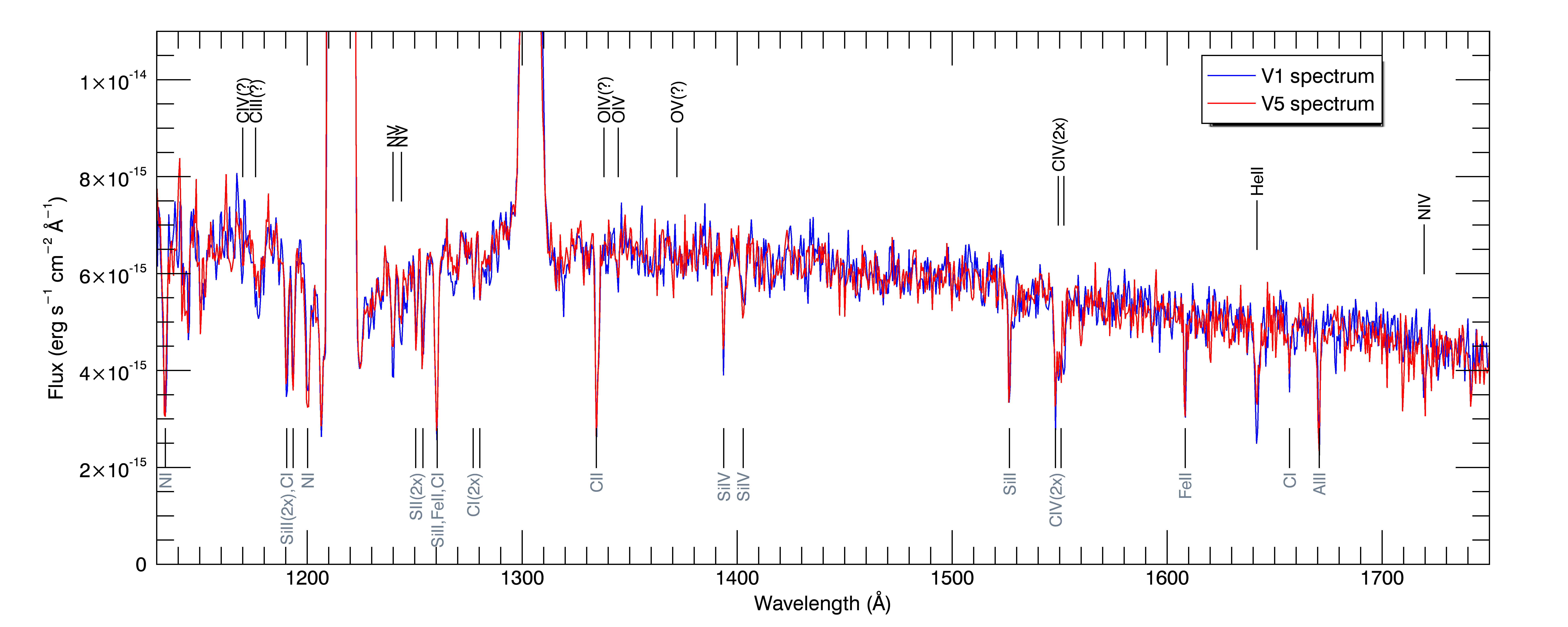
Figure 2: COS spectra of V1 and V5 (binned over six pixels for more clarity), the flux from V5 was adjusted so that the two spectra overlap. The strongest interstellar lines are indicated below the spectra while the photospheric ones are labelled above.

It is immediately apparent that several mass estimates are far too low to be reconciled with the idea that most the hot subdwarfs are helium core or post-helium core burning stars. While the six hottest stars in the sample, the hot H-rich sdOs (including four pulsators), show a reasonable mean mass of 0.452 $M_{\rm\odot}$, the rest of the sample, taken as a whole, shows an unacceptably low mean mass value of 0.331 $M_{\rm\odot}$, below the minimum mass for helium burning. Interestingly, the spectroscopically inferred low mass problem for HB and EHB stars in $\omega$ Cen has been encountered by Moehler et al. (2011) and discussed in detail by Moni Bidin et al. (2011; 2012). The problem seems to affect only that cluster in particular.

The mass distributions of the hot and cool subsamples are shown in Fig. 1. The distributions were obtained following the procedure described in Fontaine et al. (2012): individual gaussians defined by each individual value of the mass and its uncertainty are added together. Each gaussian has been normalised such that its surface area is the same for each star, thus ensuring the same weight in the addition procedure. We do not believe the increase of mass with temperature to be real, especially considering that the hot sdO stars are likely to be post-EHB objects. The mass difference would be naturally explained if the temperature of the sdO stars had been underestimated. Recomputing masses with temperatures increased by 10 000 K for the hottest stars leads to values compatible with the rest of the sample. We thus suggest that an underestimation of the effective temperature for the sdOs in the sample could explain the apparent mass discrepancy between the hot and cool samples.

Table 1: Atmospheric and other parameters for the 38 stars in the sample of Latour et al. (2014). The entries below the solid line refer to the “hot” subsample.

Identifier	$T_{\rm eff}$ (K)	log $g$	log $N$(He)/$N$(H)	$M_{B}$	$M$/$M_{\rm\odot}$
5238307	25711 $\pm$ 400	5.35 $\pm$ 0.06	$-$2.27 $\pm$ 0.08	4.428$\pm$0.147	0.231$\pm$0.102
5139614	27594 $\pm$ 468	5.48 $\pm$ 0.06	$-$3.74 $\pm$ 1.06	4.661$\pm$0.147	0.211$\pm$0.102
204071	28828 $\pm$ 602	5.53 $\pm$ 0.09	$-$3.00 $\pm$ 0.14	3.767$\pm$0.148	0.618$\pm$0.130
168035	29770 $\pm$ 454	5.38 $\pm$ 0.07	$-$3.27 $\pm$ 0.20	3.767$\pm$0.147	0.401$\pm$0.111
5262593	31161 $\pm$ 280	5.48 $\pm$ 0.05	$-$3.07 $\pm$ 0.29	3.648$\pm$0.146	0.531$\pm$0.092
5243164	32403 $\pm$ 281	5.41 $\pm$ 0.05	$-$2.65 $\pm$ 0.17	4.044$\pm$0.146	0.242$\pm$0.093
5180753	34850 $\pm$ 317	5.75 $\pm$ 0.06	$-$1.46 $\pm$ 0.06	4.238$\pm$0.147	0.466$\pm$0.101
5142999	34477 $\pm$ 392	5.67 $\pm$ 0.07	$-$1.09 $\pm$ 0.05	4.387$\pm$0.146	0.308$\pm$0.110
5222459	35008 $\pm$ 327	5.73 $\pm$ 0.05	$-$0.73 $\pm$ 0.04	4.663$\pm$0.146	0.253$\pm$0.093
5119720	35018 $\pm$ 403	5.77 $\pm$ 0.07	$-$0.81 $\pm$ 0.05	4.457$\pm$0.147	0.381$\pm$0.110
53945	35216 $\pm$ 316	5.91 $\pm$ 0.05	$-$0.61 $\pm$ 0.04	4.562$\pm$0.146	0.493$\pm$0.092
75981	35929 $\pm$ 307	5.71 $\pm$ 0.05	$-$1.05 $\pm$ 0.05	4.151$\pm$0.146	0.432$\pm$0.093
5164025	36020 $\pm$ 428	5.84 $\pm$ 0.07	$-$0.55 $\pm$ 0.05	4.716$\pm$0.146	0.315$\pm$0.110
5205350	36251 $\pm$ 335	5.54 $\pm$ 0.06	$-$0.61 $\pm$ 0.04	4.300$\pm$0.146	0.193$\pm$0.101
5165122	36331 $\pm$ 328	5.71 $\pm$ 0.06	$-$0.64 $\pm$ 0.04	4.439$\pm$0.146	0.288$\pm$0.101
165943	36479 $\pm$ 401	5.76 $\pm$ 0.07	$-$0.68 $\pm$ 0.05	4.351$\pm$0.147	0.383$\pm$0.110
5141232	36583 $\pm$ 402	5.72 $\pm$ 0.07	$-$0.61 $\pm$ 0.05	4.416$\pm$0.146	0.300$\pm$0.110
274052	36640 $\pm$ 506	5.59 $\pm$ 0.09	$-$0.35 $\pm$ 0.06	4.558$\pm$0.147	0.140$\pm$0.130
5242504	36653 $\pm$ 387	5.75 $\pm$ 0.07	$-$0.45 $\pm$ 0.05	4.495$\pm$0.146	0.298$\pm$0.110
264057	36696 $\pm$ 408	5.70 $\pm$ 0.07	$-$0.80 $\pm$ 0.05	4.421$\pm$0.147	0.280$\pm$0.111
5142638	36740 $\pm$ 428	5.71 $\pm$ 0.07	$-$0.38 $\pm$ 0.05	4.649$\pm$0.146	0.210$\pm$0.110
5102280	36948 $\pm$ 327	5.70 $\pm$ 0.06	$-$0.94 $\pm$ 0.05	4.195$\pm$0.146	0.374$\pm$0.101
177711	37093 $\pm$ 433	5.72 $\pm$ 0.07	$-$0.45 $\pm$ 0.05	4.429$\pm$0.147	0.287$\pm$0.111
5220684	37544 $\pm$ 368	5.82 $\pm$ 0.07	$-$0.86 $\pm$ 0.05	4.338$\pm$0.147	0.435$\pm$0.110
5062474	37554 $\pm$ 863	5.90 $\pm$ 0.14	$-$0.09 $\pm$ 0.09	4.757$\pm$0.148	0.330$\pm$0.183
5138707	37855 $\pm$ 599	5.93 $\pm$ 0.09	0.57 $\pm$ 0.05	4.932$\pm$0.147	0.283$\pm$0.130
5124244	38432 $\pm$ 530	5.97 $\pm$ 0.09	$-$0.01 $\pm$ 0.05	4.730$\pm$0.146	0.407$\pm$0.130
5170422	38533 $\pm$ 340	5.60 $\pm$ 0.06	$-$0.77 $\pm$ 0.04	4.190$\pm$0.146	0.240$\pm$0.101
5047695	38578 $\pm$ 549	5.69 $\pm$ 0.12	$-$0.18 $\pm$ 0.07	4.806$\pm$0.150	0.106$\pm$0.163
5085696	39072 $\pm$ 371	5.66 $\pm$ 0.08	$-$0.04 $\pm$ 0.05	4.585$\pm$0.146	0.147$\pm$0.120
5039935	39804 $\pm$ 523	6.06 $\pm$ 0.11	0.49 $\pm$ 0.07	4.998$\pm$0.148	0.353$\pm$0.151
165237	43843 $\pm$ 362	6.01 $\pm$ 0.11	0.75 $\pm$ 0.10	4.173$\pm$0.147	0.579$\pm$0.149
5242616	44959 $\pm$ 637	5.88 $\pm$ 0.08	$-$1.41 $\pm$ 0.08	4.265$\pm$0.146	0.392$\pm$0.120
5034421 (V1)	49113 $\pm$ 824	5.89 $\pm$ 0.07	$-$1.76 $\pm$ 0.09	4.137$\pm$0.147	0.408$\pm$0.112
177238 (V3)	49328 $\pm$ 877	6.07 $\pm$ 0.08	$-$1.73 $\pm$ 0.11	4.138$\pm$0.147	0.621$\pm$0.121
154681 (V4)	50635 $\pm$ 758	5.89 $\pm$ 0.08	$-$1.25 $\pm$ 0.05	4.043$\pm$0.146	0.434$\pm$0.120
281063 (V5)	58789 $\pm$ 1910	6.12 $\pm$ 0.11	$-$1.67 $\pm$ 0.13	4.344$\pm$0.147	0.487$\pm$0.152
177614	59724 $\pm$ 1288	6.02 $\pm$ 0.08	$-$1.32 $\pm$ 0.09	4.281$\pm$0.147	0.392$\pm$0.120

3 The UV analysis

3.1 Observations

Ultraviolet COS spectra of the two pulsators V1 and V5 were obtained during cycle 22 (proposal GO-13707). Each star was observed for 5337 s with the low resolution G140L (R $\approx$3000) grating in time-tag mode. The data were reduced following the standard CALCOS procedure.

The resulting spectrograms of both stars are shown in Fig. 2, where the flux of V5 was multiplied by a factor 1.138 in order to match the flux of V1, thus emphasing the similarity between the spectra of both stars. This is somewhat expected given that the pulsators form a rather homogeneous group according to the optical analysis. We can also note that the shape of the continuum is essentially the same for both stars. Since this is largely due to interstellar reddening, it is not surprising that it is very similar for the two targets. Most of the strong spectral features are due to the interstellar medium and are labelled below the spectra in Fig. 2; C i-ii, N i Si II, Fe II and Al II, also conspicuous are the Ly$\alpha$ and O i ($\lambda$1304) geocoronal emission lines. The Si iv resonance doublet ($\lambda\lambda$1394,1403) is also visible in both stars at a radial velocity (RV) consistent with zero, thus indicating its interstellar origin. No stellar component can be resolved for this doublet. As for the C iv resonance lines ($\lambda\lambda$1548,1551), both the interstellar (RV $\approx\-$20 km s^-1) and photospheric components (RV $\approx$230 km s^-1) can be resolved. Additional photospheric lines are the N v resonance doublet ($\lambda\lambda$1239,1243), N iv $\lambda$1718 and He ii $\lambda$1640, which are found at a radial velocity consistent with that of the cluster (232 km s^-1, Harris 1996).

3.2 The COS light curves

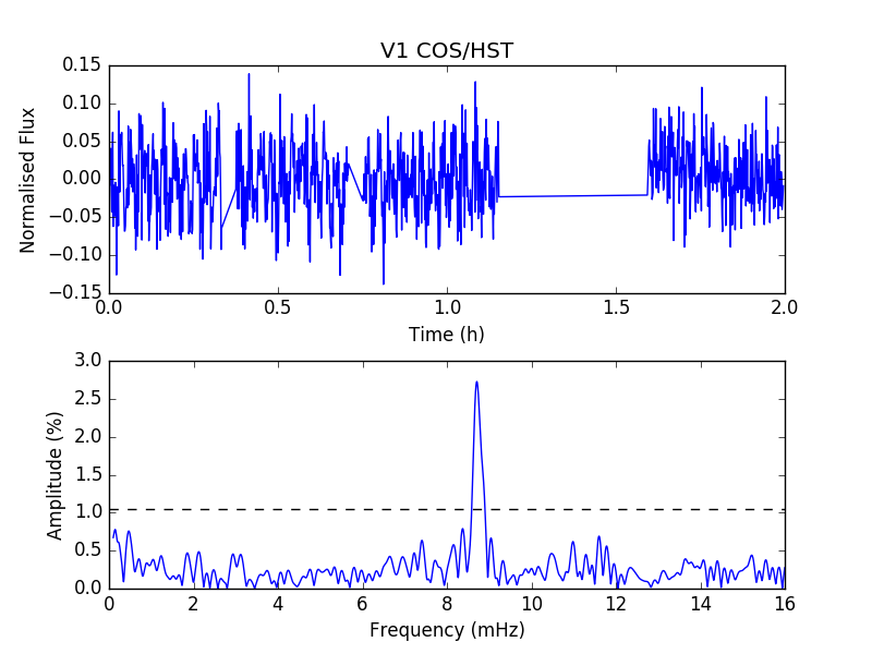
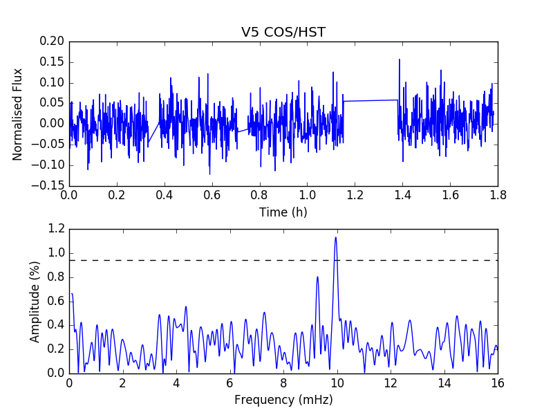
Figure 3: Light curves and Fourier amplitude spectrum corresponding to the COS observations of V1 and V5. The horizontal dashed line indicates the 3.5$\sigma$ detection threshold.

We took advantage of the time-tag mode to construct the UV light curves of both stars using the LightCurve tool, a discussion on the method is presented in Sandhaus et al. (2016). The time-tag counts were binned into datachunks of 5 s. This is small enough to fully resolve the expected pulsations in the $\approx$80-120 s range while still giving adequate S/N in each data point.

The top panels of Figure 3 show the light curves obtained for the two stars, normalised to the average flux of the star in question. They are each divided into four chunks of continuous data, corresponding to observations at the four COS FPOS positions. The large gap in each curve represents the re-acquisition period.

The lower panels of Figure 3 show the Fourier amplitude spectrum based on the COS lightcurves. Periodicities with amplitudes above the 3.5 $\sigma$ threshold were extracted at 114.8 s (2.7% amplitude) and 113.4 s (1.2% amplitude) for V1, and at 100.5 s (1.1% amplitude) for V5. These periods correspond well to the dominant modes known for these stars from ground-based optical time-series photometry (Randall et al. 2016, 2011). For V5, an additional period known from the optical data is also recovered just below 3.5 $\sigma$ at 107.8 s (0.6% amplitude).

While it is interesting to compare the observed periodicities and amplitudes derived from the optical and the COS data at the qualitative level, a quantitative comparison is not particularly instructive due to the very different time baselines of the datasets. Indeed, for V1 the optical $u^{\prime}$-band light curve obtained over a 6-day period in 2009 yields a rather messy Fourier spectrum with several closely split components clustered around 115.0 s, 114.7 s and 114.4 s (see Table 4, Randall et al. 2016), whereas an earlier $B$ band dataset taken over two nights in 2009 shows dominant periods at 114.7 s and 113.7 s (see Table 1, Randall et al. 2011), very similar to those uncovered with COS. It is not clear which of the split components constitute independent harmonic oscillations and which are induced in the Fourier spectrum, for example by intrinsic amplitude variations or the beating of closely spaced modes. The longer the time baseline and the better the quality of the data, the more complicated the Fourier spectrum appears to become. For V5 the situation seems simpler, the previously extracted 100.6 s, 99.3 s and 107.5 s periodicities (Randall et al. 2016) not being split in any obvious way, but this is likely due to the much lower pulsational amplitudes and the limited S/N of the data.

Given the clear indications for pulsational amplitude variability there is no point in trying to use the relative amplitudes observed in the different frequency bands for mode identification. If simultaneous time-series photometry were available it would in principle be possible to exploit the colour dependence of each mode’s amplitude to derive the degree index $\ell$, as has been done with some success for rapidly pulsating sdB stars in the field (Randall et al. 2005). Since in our case the different datasets are taken several years apart we limit ourselves to a very qualitative comparison of the apparent amplitudes in the different bands. For the low-degree modes expected to be observed in these stars we would expect a general trend of amplitude decrease with increasing wavelength, that is, the apparent COS far-UV amplitudes should be significantly higher than those seen in the optical data (assuming a similar intrinsic amplitude of the mode at the time of observation) due to the frequency-dependence of the limb darkening (see Randall et al. 2005, for details). This is assuming these stars behave similarly to the much cooler pulsating sdB stars, since detailed calculations of the pulsational perturbation of the stellar atmosphere have not yet been carried out for sdO stars.

In our very rudimentary colour-amplitude analysis we simply add up the amplitudes of all frequency components around the 115 s complex for V1. This gives a far-UV amplitude of 3.9%, a $u^{\prime}$ amplitude of 5.1% and a $B$ amplitude of 2.2%. For the 100.6 s pulsation in V5 we find 1.1% in the far-UV vs 0.54 % in the $u^{\prime}$, and for the 107.5 s pulsation we have 0.6% in the far-UV and 0.42 % in the $u^{\prime}$ (no $B$-band data are available for this star). With the exception of the very large $u^{\prime}$ amplitude derived for the 115 s complex in V1 (that value is particularly unreliable due to the many split components), the general trend does seem to be for the UV amplitudes to be larger than the corresponding peaks in the optical. However, given the small number statistics this is not a significant result, and it is not clear how indicative the amplitudes derived from the $u^{\prime}$ and $B$ bands are. We would expect the amplitude from the ground-based optical data to underestimate the true apparent amplitudes due to the flux contribution from nearby (presumably not pulsating) stars in the very crowded $\omega$ Cen field. This is true in particular for V5, which has a very close relatively bright companion. We tentatively conclude that the far-UV amplitudes observed in the $\omega$ Cen variables appear qualitatively comparable to or up to twice as large as those from ground-based optical data. This finding is of interest in the context of comparing the far-UV space-based pulsational properties of hot subdwarfs (such as those obtained for the pulsators in NGC2808 by Brown et al. 2013) to those derived from ground-based optical data.

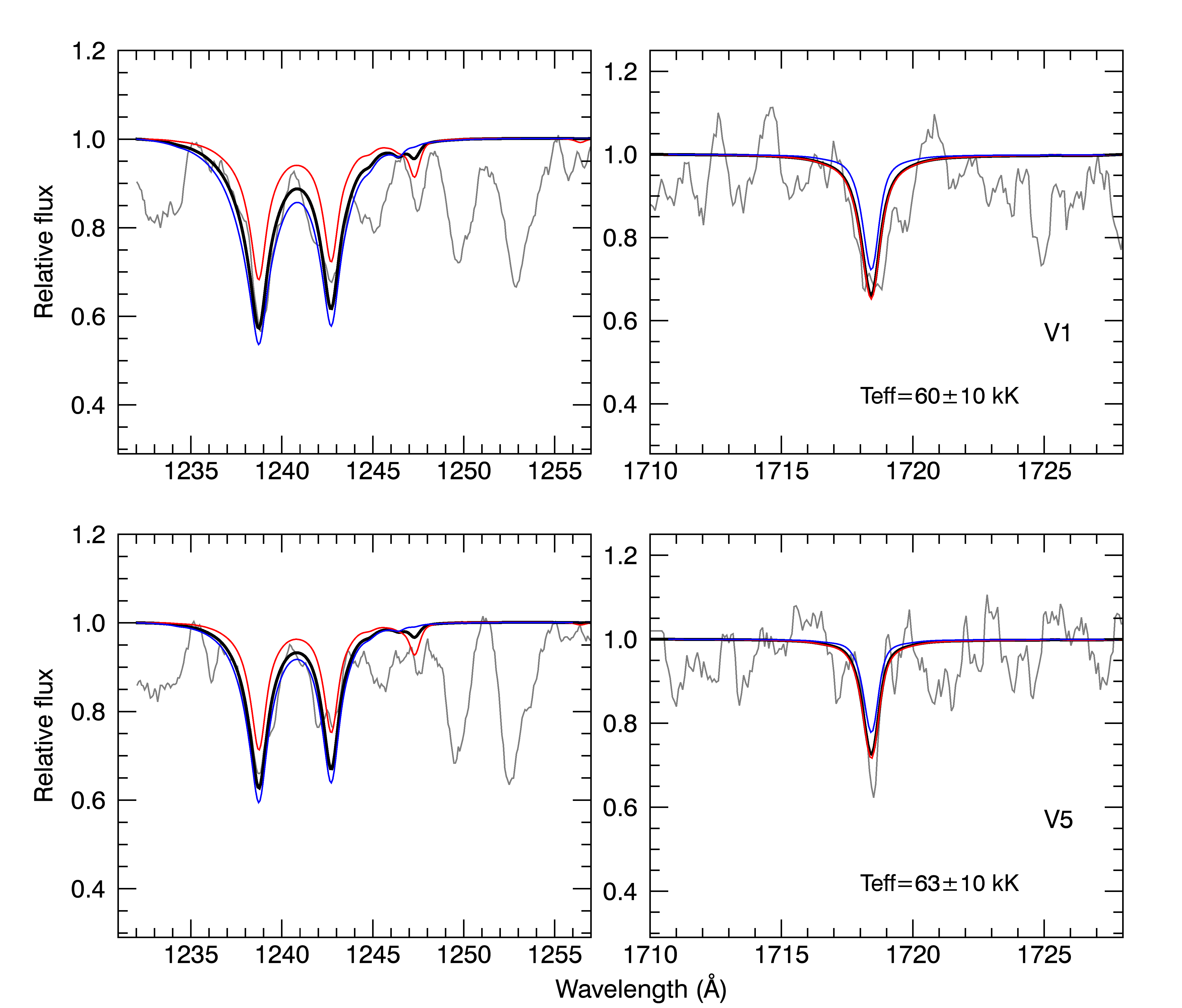
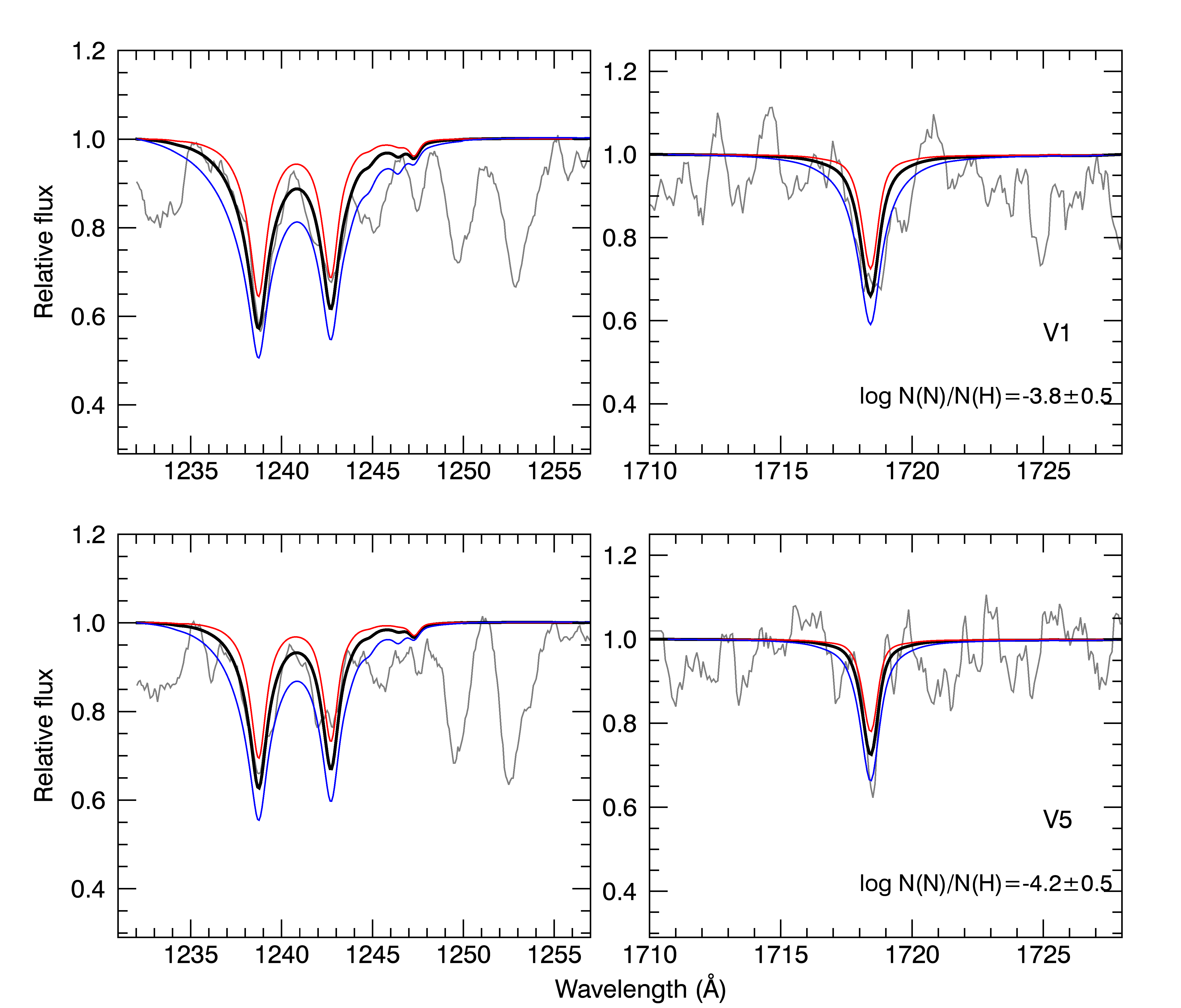
Figure 4: Best fitting models (thick black line) for the N v doublet and N iv line in the spectrum of V1 (upper panels) and V5 (lower panels). The observed spectra (grey) are smoothed over a six pixels width (one resolution element) in this figure and the following ones. Right panels: As a comparison, model spectra with a lower (red) and higher (blue) temperature are shown. Left panels: With model spectra having a lower (red) and higher (blue) nitrogen abundance.

3.3 Analysis of the COS spectra

Our goal was to use strong metal lines in the UV range to simultaneously determine the metal abundance and the temperature, using lines originating from different ionization levels. In the observed wavelength range ($\approx$1150$-$2000 Å), lines originating from C iii-iv, N iv-v and O iv-v are predicted. As already mentioned, we detect the nitrogen lines and the C iv doublet in our spectra. Unfortunately, the C iii multiplet ($\approx$1176 Å) and the C iv lines (1169 Å) cannot be used for the analysis. A wide absorption feature between $\approx$1170-1180 Å is seen in both spectra (and indicated in Fig. 2), hiding any hints of the C iii multiplet. We could not find the origin of this feature. No strong interstellar lines are expected in this region and we verified that no artefact was produced when combining the four subexposures. Iron and nickel lines can be abundant at these wavelengths but are not expected to produce such a strong feature. To nevertheless examine this possibility we compared an IUE spectrum (degraded to the COS resolution) of Feige 34 with our COS spectra, but did not find any similar feature. Feige 34 is an sdO star with parameters, to our best knowledge, similar to those of V5 but enriched in iron and nickel (Latour et al. 2016). If those lines were at the origin of the feature seen in the COS spectra, we would expect it to feature even more prominently in the IUE spectrum of Feige 34. Although the COS handbook mentions calibration issues at these wavelengths, the same phenomenon was seen by Brown et al. (2012) (see their figure 12) with STIS/G140L spectra of EHB stars, suggesting that there might be an unknown astrophysical explanation. Finally, a firm identification of the oxygen lines (1338 Å, 1342 Å, and 1371 Å) was not possible, suggesting a sub-solar abundance. Thus we had to rely on the nitrogen lines for our analysis.

For each star we built a two-dimensional grid of NLTE model atmospheres, varying $T_{\rm eff}$ and the nitrogen abundance, while keeping the other parameters fixed. For both stars the grid covered the following ranges: $T_{\rm eff}$ from 45 000 K to 65 000 K in steps of 2 000 K and log $N$(N)/$N$(H) from $-$3.0 to $-$5.8 in 0.4 dex intervals. The surface gravity and helium abundance were fixed for each star to the values derived by the optical analysis (see Table 1). The model atmospheres and synthetic spectra were computed with the public codes TLUSTY and SYNSPEC (Lanz & Hubeny 2003, 2007), and include C, N, and O as metallic elements in addition to H and He. We adopted in these models a carbon abundance of log $N$(C)/$N$(H)=$-$4.6, according to the estimates from the optical spectra (Latour et al. 2014), and an oxygen abundance of one tenth solar, given the weakness of the observed oxygen features. Because the line spread function of COS departs from the usual Gaussian function, we used the theoretical profiles listed on the COS website (G140L/1105 at lifetime position 3) for the convolution of our synthetic spectra.

We then used our synthetic spectra grids to simultaneously fit the nitrogen lines in the observed spectra. The result can be seen in Fig. 4, where the thin grey line represents the observation, while the thick black line is a best fitting model. In the case of V1 we obtained values of log $N$(N)/$N$(H) = $-$3.8$\pm$0.5 dex and $T_{\rm eff}$ = 60 000 $\pm$ 5 000 K. The nitrogen lines in V5 being less strong, the fit for this star resulted in a lower N abundance of log $N$(N)/$N$(H) = $-$4.2$\pm$0.5 dex combined with $T_{\rm eff}$ = 63 000 $\pm$ 6 000 K. The line profiles are not very well defined at low resolution, and the SNR is relatively low in the 1718 Å region, which explains the rather high uncertainties. Nevertheless, the nitrogen lines indicate effective temperatures higher than the optical estimates (by $\approx$10 000 K for V1 and $\approx$5 000 K for V5). The nitrogen abundances are consistent with a solar value ($-$4.2) which is rather typical for hot subdwarf stars (Blanchette et al. 2008; Geier 2013). For comparison, in Fig. 4 we overplot the N line profiles for temperatures of $\pm$10 kK than those obtained with the fit on the left panels. As seen from the figure, the N iv line is not sensitive to temperature below $\approx$63 kK, while the N v doublet appears too weak at lower $T_{\rm eff}$. At the lower temperatures, the higher N abundance required to match the N v lines would produce a N iv line stronger than observed. The effect of changing the nitrogen abundance by $\pm$0.5 dex is shown on the right panels of Fig. 4.

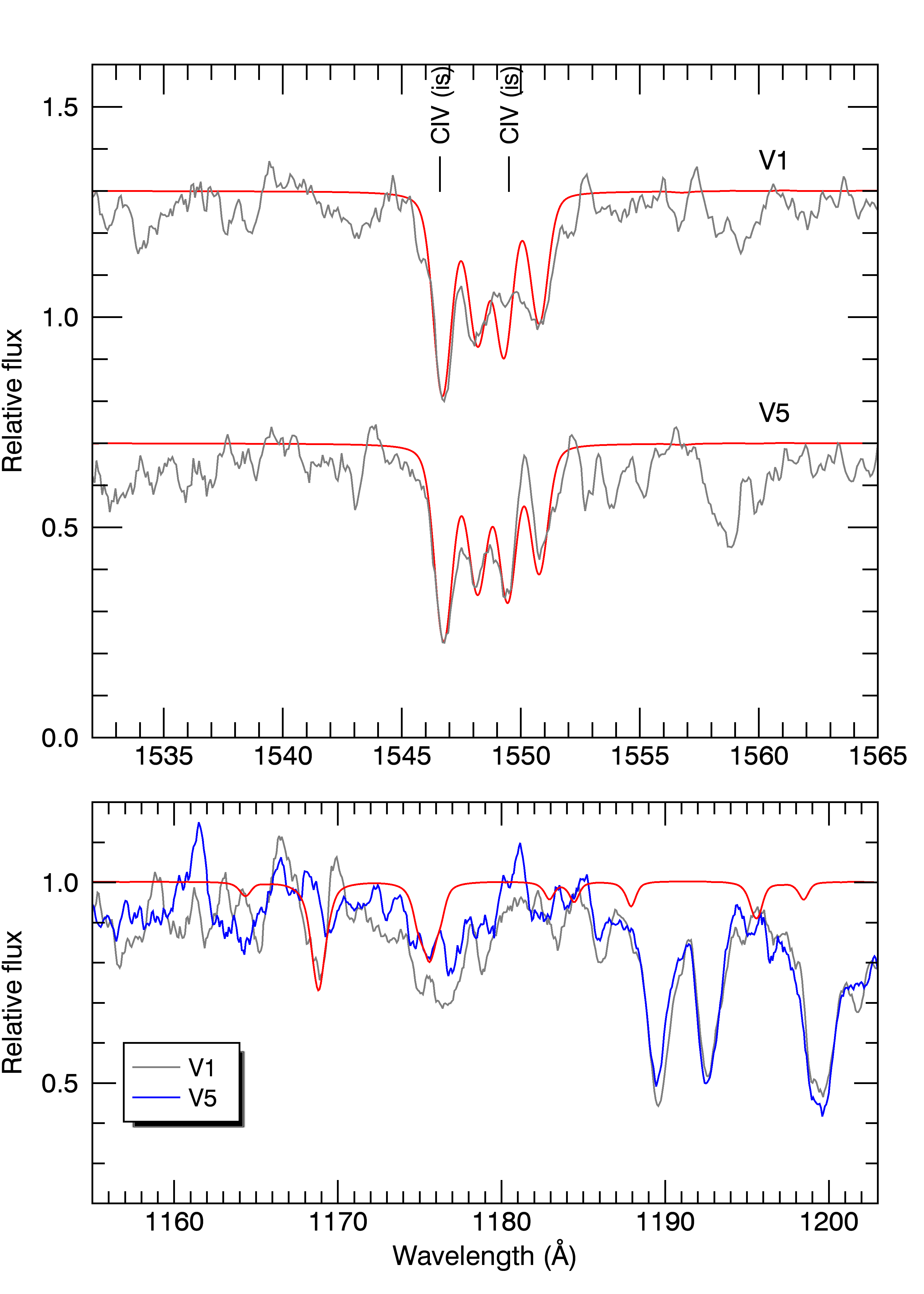
Figure 5: Upper panel : Comparison between the observed (grey) spectra of V1 and V5 in the C iv doublet region and synthetic spectra combining interstellar and photospheric lines (red). The normalized spectra are shifted along the $y$ axis for better visualization. Lower panel: The region of the C iv (1169 Å) and C iii ($\approx$1176 Å) lines is shown for V1 and V5. A theoretical spectrum is shown in red as comparison.

Similar temperature $-$ abundance grids were made for oxygen and carbon in order to estimate their abundances. We examined the 1330-1380 Å region where the strongest oxygen lines are predicted. The only line that could be identified in both stars is the O iv at 1342 Å. The other lines are not adequately defined to claim a real detection. Nevertheless, we can set an upper limit on log $N$(O)/$N$(H) $\approx$ $-$4.6. We recall here the solar abundance to be $-$3.3 dex, so the stars would have abundances below 1/10 solar, which is also a normal value for hot subdwarfs. Considering carbon, although the IS and photospheric components of the C iv doublet can be distinguished, the line profiles are blended. However, the line strength remains in agreement with the upper limits placed from the optical spectra, log $N$(C)/$N$(H)$\lesssim$ $-$4.6 (no carbon lines are distinguishable in the optical). The upper panel of Fig. 5 shows the observed and modelled carbon doublet (interstellar and stellar components) for V1 and V5. In the lower panel, we show the observed spectra in the $\approx$1175 Å region as well as a theoretical spectrum representative for both stars. The issue of the C iii multiplet has been discussed previously, and the plot clearly illustrates that the predicted carbon line cannot explain the observed feature around 1175 Å.

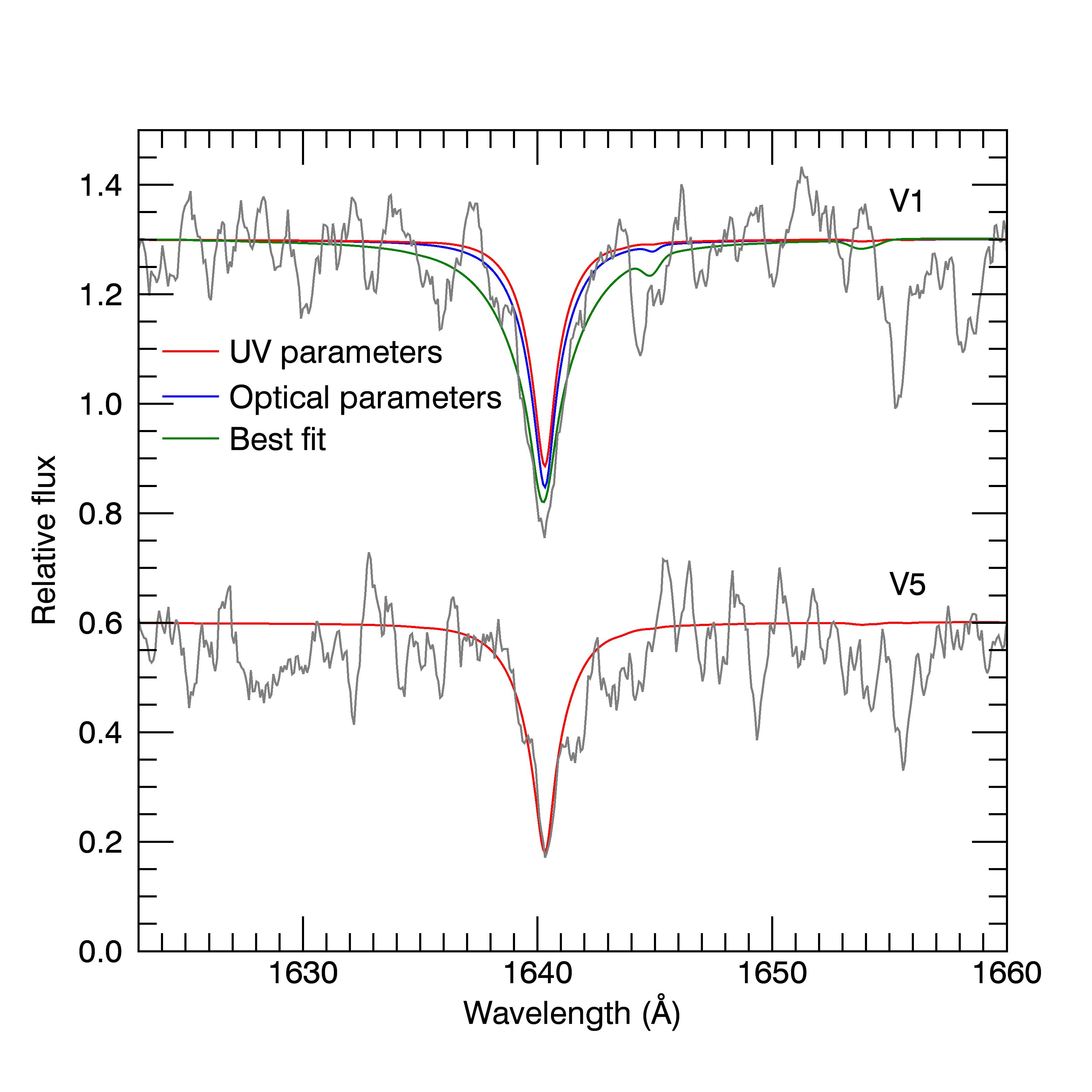
Figure 6: Comparison between the observed He ii $\lambda$1640 line (grey) for V1 and V5 and synthetic spectra at their UV optimal temperature (red). For V1 we added also a model at the optical determined temperature (blue) and the best fit model to the line (green).

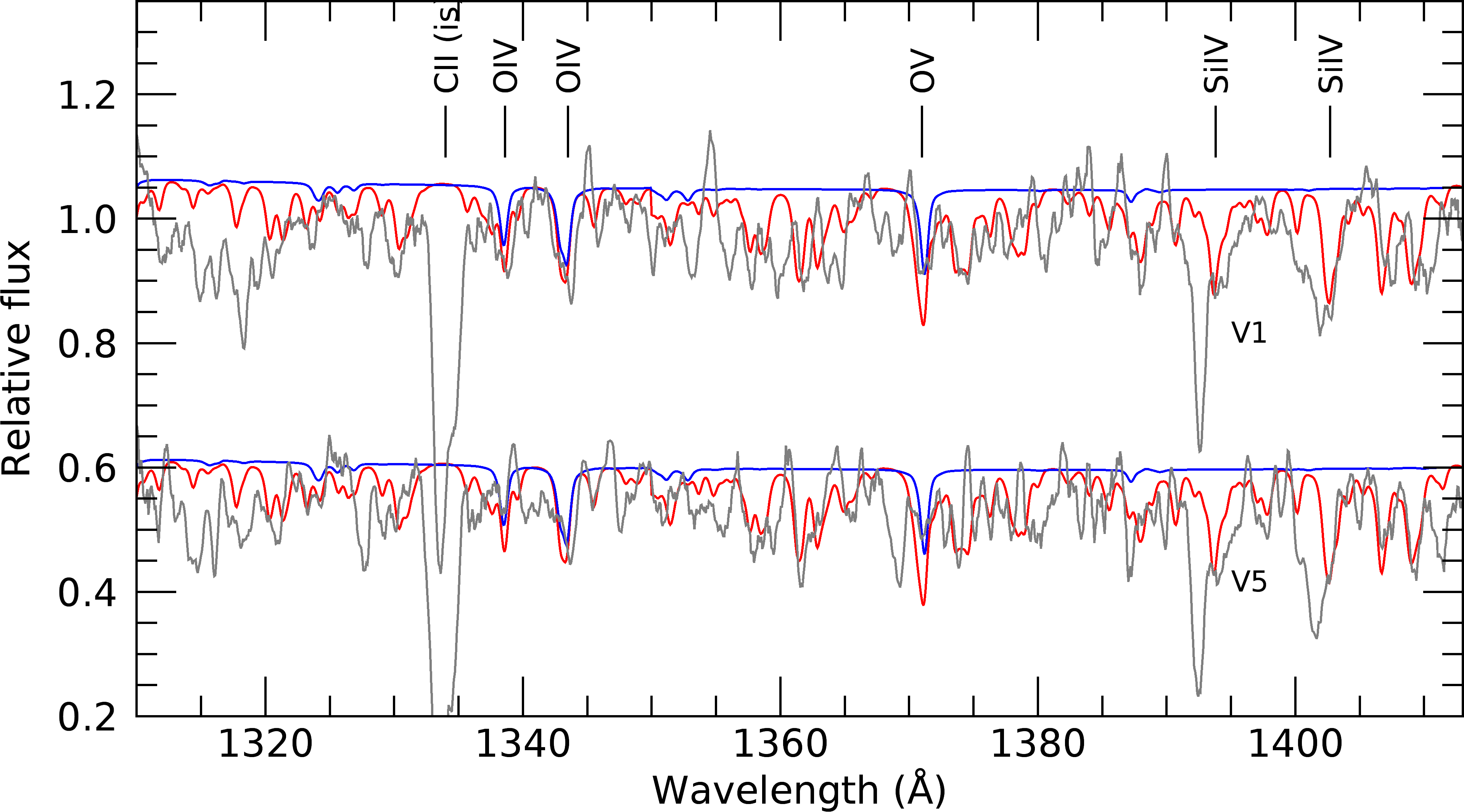
Figure 7: COS spectra of V1 and V5 (grey) compared with model spectra including C, N, and O at their derived values (blue) and an additional solar amount of Fe and Si (red)

.

The final photospheric feature visible in the spectra is the He ii line at 1640 Å. Figure 6 shows the region surrounding this line in the COS spectra of V1 and V5, overplotted (red) by synthetic models with a $T_{\rm eff}$ of 60 and 63 kK respectively. For V5, we have a good match between the synthetic and observed spectra, while for V1 the observed He ii line is too strong to be reproduced by the synthetic spectrum. This is somewhat unexpected since the helium abundance derived from the optical spectra is very similar for both stars (log $N$(He)/$N$(H) = $-$1.76 and $-$1.67 for V1 and V5 respectively). The effective temperature affects the strength of the He lines, but in the $T_{\rm eff}$ range of our stars the effect is not very strong for $\lambda$1640. This is illustrated with the blue curve in Fig. 6 which shows the He line at $T_{\rm eff}$ = 49 000 K (the value derived from the optical spectra, see Table 1). The He ii line is indeed stronger at lower $T_{\rm eff}$, but still not strong enough to match the observed profile which is wider and deeper still. We also fit the He ii line of V1 in the temperature$-$helium abundance parameter space. The resulting best fit is illustrated by the green curve in the plot, corresponding to the following parameters: $T_{\rm eff}$ = 51 000 $\pm$ 4000 K and log $N$(He)/$N$(H) = $-$0.76 $\pm$ 0.3. This helium abundance is ten times higher than the one indicated by the optical spectrum and thus in serious contradiction; such an abundance would produce optical helium lines that are much stronger than observed. Moreover the theoretical line profile does not fit the UV spectrum very well, the wings being too broad and the core not deep enough. To conclude, we do not understand the He ii line in the COS spectrum of V1.

As mentioned previously, the silicon resonance lines have RVs indicating an interstellar origin with no resolved photospheric components. Individual lines from heavy elements like iron and nickel can also not be resolved at the low resolution and relatively poor S/N of our spectra. However, by comparing the COS spectra with model spectra including a solar amount of silicon and iron, we found such abundances to be compatible with our observations. Thus, a solar abundance is a reasonable upper limit to place on these elements.

Figure 7 displays our observed spectra over a spectral range especially rich in Fe v lines. Overplotted in red are model spectra for both stars including silicon and iron at solar abundances (C, N, O are also included at their estimated values). Oxygen and silicon lines are indicated, while the other features are due to iron, as comparison, model spectra without Si and Fe are plotted in blue. We note that the O v $\lambda$1370 line is blended with iron lines present at its blue side, which makes it appear stronger in a model including iron.

4 Conclusion

We addressed the issue of the temperature discrepancy of the $ω$ Cen instability strip discussed in Randall et al. (2016). As shown in their Figure 11, the pulsating sdOs are found at temperatures cooler than the predicted instability region favourable to pulsations. The discrepancy could be explained either by shortcomings in the seismic models (e.g. nickel opacity might boost pulsations at lower effective temperatures) or by an underestimation of the surface temperature of the stars derived by means of optical spectroscopy. In this paper, we focussed on the second possibility by analysing low resolution COS spectra of two pulsators (V1 and V5). We also determined a mass distribution for the sample of EHB stars presented in Latour et al. (2014).

From the mass distribution, we noticed a significant difference between the mean mass of the ”cool” stars of the sample (with $T_{\rm eff}$$\buildrel<\over{\sim}\$ 45 kK) and the hotter sdOs. The latter group includes only six stars (including four of the pulsators) but the mean mass difference of 0.127 $M_{\rm\odot}$ is nevertheless suspicious. This mean mass discrepancy could indicate that the effective temperatures are underestimated from the optical spectra, since an increase in the temperature of the stars would lead to a lower radius (and mass) needed to match the observed magnitude of the stars, given a fixed distance to the cluster.

To investigate the issue in more detail, we analysed low resolution UV spectra for two of the pulsators, namely V1 and V5. The goal was to use the ionization equilibrium of strong metal lines (C, N, O) originating from different ionic states to assess more precisely the effective temperature of the stars. However, only the nitrogen lines could be used to this purpose. From the N v doublet and N iv $\lambda$1718 lines we could estimate the nitrogen abundances to be close to solar for V5 and slightly higher in V1. Given these nitrogen abundances, the observed strength of the N v doublet indicates temperatures significantly higher than those estimated from optical spectroscopy. For V1 we obtained $T_{\rm eff}$ = 60$\pm$5 kK and a slightly higher temperature of $T_{\rm eff}$ = 63$\pm$6 kK for V5. The uncertainties are rather large given that we are forced to rely on three spectral lines in low quality spectra, but it is nevertheless quite clear that the nitrogen lines require the effective temperature to be closer to 60 kK than 50 kK for both stars. As for other elements, the strength of the C iv doublet is consistent with the upper limit derived from the optical spectra of about 1/10 solar and the oxygen abundance is also depleted by at least a factor of 10 with respect to solar. Upper limits for silicon and iron are about solar.

In summary, based on the mass distribution of the $ω$ Cen sdOs, and the UV nitrogen lines of the two pulsating stars V1 and V5, it is likely that the effective temperatures of the sdOs in the $\omega$ Cen sample are systematically higher than those derived from the optical spectra, thus moving the stars into the instability region predicted by seismic models. Our analysis was however limited by the quality of the data available. The analysis and parameter determination of hot stars (sdOs, white dwarfs) is hampered by inherent difficulties, such as the behaviour of the Balmer lines and the weak temperature dependence of the UV and optical flux distribution. Combining these issues with the observational difficulties faced for faint stars in a very crowded field makes studies such as that attempted here very challenging indeed. We believe the most promising way forward is to conduct spectroscopic studies of brighter stars with effective temperatures similar to the $ω$ Cen sdOs. This could go a long way towards an understanding of the fundamental parameters of these stars and how to reliably derive them, as well as their chemical patterns and evolutionary status.