Diffusion in systems crowded by active force-dipole molecules

Abstract

Experimental studies of systems containing active proteins that undergo conformational changes driven by catalytic chemical reactions have shown that the diffusion coefficients of passive tracer particles and active molecules are larger than the corresponding values when chemical activity is absent. Various mechanisms have been proposed for such behavior, including, among others, force dipole interactions of molecular motors moving on filaments and collective hydrodynamic effects arising from active proteins. Simulations of a multi-component system containing active dumbbell molecules that cycle between open and closed states, a passive tracer particle and solvent molecules are carried out. Consistent with experiments, it is shown that the diffusion coefficients of both passive particles and the dumbbells themselves are enhanced when the dumbbells are active. The dependence of the diffusion enhancement on the volume fraction of dumbbells is determined, and the effects of crowding by active dumbbell molecules are shown to differ from those due to inactive molecules.

I Introduction

A body of evidence points to the existence and importance of nonthermal fluctuations in the cell that are driven by chemical activity that maintains the cell in a nonequilibrium state. Caspi et al. (2000); Lau et al. (2003); MacKintosh and Levine (2008); Wilhelm (2008); Gallet et al. (2009); Weber et al. (2012); Bruinsma et al. (2014); Guo et al. (2014) Such fluctuations have been measured and characterized using various experimental probes and are often attributed to the forces generated by molecular motors when they interact with filaments comprising the cellular cytoskeletal network. The results of in vitro experiments on systems containing actin networks and active myosin motors also suggest that nonthermal fluctuations play a significant role in the systems’ dynamical response to deformation. Mizuno et al. (2007); Toyota et al. (0011) Support for such effects is provided by the observation that the mean square displacements of passive molecules and active species are smaller when the production of ATP is inhibited. For example, the diffusive dynamics of chromosomal loci in prokaryotic cells is sensitive to metabolic activity; when ATP synthesis is inhibited the apparent diffusion coefficient decreases. Weber et al. (2012) Force-spectrum-microscopy studies have shown that force fluctuations in eukaryotic cells enhance the movement of large and small molecules; when the activity of myosin II motors is selectively inhibited diffusive motion decreases but not to the degree when all ATP synthesis is suppressed. Guo et al. (2014) These studies have concluded that it is the aggregate of all metabolic activity, and not just that of motor proteins, that contributes to enhanced diffusive motion.

Enhanced diffusion of enzymes and passive particles has also been observed in in vitro studies of active enzymes in solution where motor proteins are not present Muddana et al. (2010); Sengupta et al. (2013); Pavlick et al. (2013), and the possible origins of these effects have been discussed Golestanian (2015). Proteins executing conformational changes as a result of catalytic chemical activity can give rise to collective hydrodynamic effects that enhance the diffusion of both passive particles and enzymes. Mikhailov and Kapral (2015); Kapral and Mikhailov (2016); Koyano et al. (2016) On more macroscopic scales, and in a somewhat different context, experimental and theoretical investigations of the diffusion coefficients of passive particles in suspensions of active microorganisms have shown diffusion enhancement due to the hydrodynamic flow fields generated by their swimming motions. Kim and Breuer (2004); Leptos et al. (2009); Mino et al. (2013); Saintillan and Shelley (2012); Kasyap et al. (2014)

In this paper we investigate diffusive dynamics in a system containing active dumbbell molecules, a passive particle and solvent. The active dumbbell molecules cycle between open and closed conformations and act as nonequilibrium fluctuating force dipoles. The microscopic dynamics accounts for direct hydrodynamic interactions as well as direct interactions among the dumbbell molecules. Molecular crowding is known to influence the diffusive properties of tracer particles in solutions where the concentration of crowding species is high: subdiffusive dynamics is observed on intermediate time scales and long-time diffusion coefficients decrease as the concentration of crowding elements increases. Metzler and Klafter (2000); Schnell and Turner (2004); Höfling and Franosch (2013); Nakano et al. (2014); Kuznetsova et al. (2014) Our investigations show how the diffusive dynamics of passive particles, and the dumbbells themselves, vary with the volume fraction of active dumbbell molecules. Comparisons with the results for the diffusive dynamics in systems containing inactive dumbbells allow us to analyze and describe the effects of dumbbell activity.

The outline of the paper is as follows. Section II describes the system under study, including the active dumbbell-shaped “molecules”, the interaction potentials among species and the dynamical method used to evolve the system. The properties of single active and inactive dumbbell molecules are presented in Sec. III. Systems containing many active dumbbell molecules are considered in Sec. IV, where simulation results for the self-diffusion coefficients of the passive particle and dumbbell molecules are given as a function of the dumbbell force constants and volume fractions. The conclusions of the study are given in Sec. V.

II System and dynamical model

The entire system is comprised of dumbbell-shaped active molecules, a passive particle and solvent molecules. The dumbbell-shaped molecules consist of two beads linked by a harmonic bond, with interactions between beads of different dumbbells described by the steep repulsive potential function Padding and Louis (2006),

$$U_{cc}=4\epsilon\left[\left(\frac{\sigma_{c}}{r}\right)^{48}-\left(\frac{\sigma_{c}}{r}\right)^{24}+\frac{1}{4}\right]\;\;r\leq 2^{1/24}\sigma_{c},$$ (1)

and zero otherwise, where $\epsilon$ sets the energy scale, which we take to be $\epsilon=2.5\;k_{B}T$ throughout, with $k_{B}$ the Boltzmann constant and $T$ the temperature. The passive particle is a structureless bead of diameter $\sigma_{c}$ and mass $m_{c}$, and interacts with the dumbbell beads through the potential in Eq. (1). The passive particle interacts with the solvent particles through the repulsive Lennard-Jones interaction potential $U_{cf}$, given by

$$U_{cf}=4\epsilon\left[\left(\frac{\sigma_{cf}}{r}\right)^{12}-\left(\frac{\sigma_{cf}}{r}\right)^{6}+\frac{1}{4}\right]\;\;r\leq 2^{1/6}\sigma_{cf},$$ (2)

and zero otherwise, where $\sigma_{cf}$ is the passive particle-solvent interaction distance.

Other interactions involving the solvent are taken into account through multiparticle collision (MPC) dynamics, comprising streaming and collision steps. Malevanets and Kapral (1999); *ref:SRD2; Kapral (2008); Gompper et al. (2009) The solvent molecules are represented by point particles of mass $m_{f}$ which are evolved in the streaming step, either ballistically or, when potential interactions are present, by Newton’s equations of motion. In the collision steps, which occur at time intervals $\tau_{{\text{M}PC}}$, the solvent particles are sorted into cubic collision cells with length $a$, in which they interact with each other according to multiparticle collisions. The coupling of the dumbbell to the solvent also can be accounted for in this way, where the constituent spheres of the dumbbell are included with the solvent particles in the collision step, in the same manner as for single polymers Mussawisade et al. (2005); Ripoll et al. (2006). Further simulation details on the implementation of the MPC algorithm, along with parameter values, are given in Appendix A.

Dumbbell molecule

While the dumbbells are fictitious ”molecules” their dynamics is constructed to mimic the conformational changes that occur in active enzymes. Kogler (2012); Mikhailov and Kapral (2015) Many catalytically active proteins cycle between open and closed conformations: substrate binding triggers passage from the open to closed state, while substrate unbinding or product release causes the protein to return to its open conformation. Such systems are maintained in a nonequilibrium state by input of substrate and removal of product.

The dumbbell beads, each with mass $m_{b}$, are linked by a harmonic bond that specifies open (large bond rest length) and closed (small bond rest length) conformations. The bond potential energy function has the form,

$$U=\displaystyle\frac{1}{2}k_{0}(t)\left(\ell-\ell_{0}(t)\right)^{2},$$ (3)

where the bond rest length $\ell_{0}(t)$ and force constant $k_{0}(t)$ are dichotomous random variables that take the two values $\{\ell_{o},\ell_{c}\}$ and $\{k_{o},k_{c}\}$. These correspond to the values for the open and closed configurations, respectively. A stochastic process that switches the dumbbell between the open and closed states is as follows: suppose the current rest bond length is $\ell_{c}$. If during the evolution the bond length $\ell$ crosses a threshold and satisfies the condition $\ell<\ell_{c}+\delta\ell_{c}$, a random time $t_{h}$ is drawn from a log-normal distribution with average $t_{c}$. The rest length and force constant will remain as $\ell_{0}(t)=\ell_{c}$ and $k_{0}(t)=k_{c}$ for this time, after which $\ell_{0}(t)$ is set to $\ell_{o}$ and the force constant to $k_{0}(t)=k_{o}$. Similarly, if $\ell>\ell_{o}-\delta\ell_{o}$, $\ell_{0}(t)$ is set to $\ell_{0}(t)=\ell_{c}$ and $k_{0}(t)$ to $k_{c}$ after a randomly chosen time $t_{h}$ with average $t_{o}$. This model captures the gross features of active proteins that adopt open and closed metastable conformations and operate though Michaelis-Menten kinetics, $E+S\mathrel{\mathop{\kern 0.0pt{\rightleftharpoons}}\limits^{{\mathrm{k}_{1}}}_{\mathrm{k}_{-1}}}C\stackrel{{\scriptstyle\mathrm{k}_{cat}}}{{\rightarrow}}E+P$, where $E,\;S,\;C$ and $P$ represent the enzyme, substrate, enzyme-substrate complex and product, respectively, with excess substrate supplied and product removed.

We shall call dumbbells that undergo such nonequilibrium cyclic conformational changes active dumbbells. If instead the stochastic mechanism responsible for these changes is absent and only thermal fluctuations are present, the dumbbells will be termed inactive dumbbells. In our model, the inactive dumbbells will simply fluctuate around the open conformation. This corresponds to a system where enzymes are not supplied with substrate and remain in open conformations.

Units and parameters

Results are reported in dimensionless units: lengths are scaled by the MPC cell size $a$, masses by the solvent particle mass $m_{f}$, energy by $k_{B}T$ and time by $(a^{2}m_{f}/k_{B}T)^{1/2}$. The spring constant $k$ is in units of $k_{B}T/a^{2}$. In the simulations presented below we set $t_{o}=0$ and vary $t_{c}$, the average time spent in the closed conformation. Furthermore, we let $k_{o}=k$ and choose $k_{c}=2k$ and $\ell_{c}=\ell_{o}/2$. Our choice of $t_{o}=0$ corresponds to a system with excess substrate and reaction rates $\mathrm{k}_{1},\;\mathrm{k}_{cat}\gg\mathrm{k}_{-1}$. The closed and open dumbbell bond lengths used in all of the simulation results are $\ell_{c}=2$ and $\ell_{o}=4$, respectively, and $\delta\ell_{c}=\delta\ell_{o}=0.05(\ell_{o}-\ell_{c})=0.1$. Solvent conditions will be indicated by the value of $\tau_{{\text{M}PC}}$. Unless stated otherwise, simulations use $\tau_{{\text{M}PC}}=0.01$, but some results will be presented for $\tau_{{\text{M}PC}}=0.05$ to explore the effects of different solvent conditions (see Appendix A).

III Properties of single active and inactive dumbbells

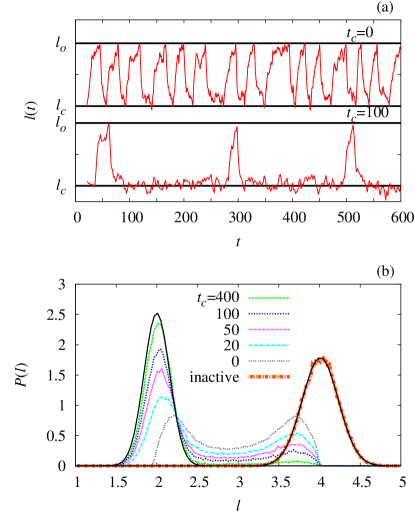
Figure 1: (a) Plot of the instantaneous bond length $\ell(t)$ against time $t$ for an active dumbbell with force constant $k=20$. Results are presented for system with average hold times $t_{c}=0$ (top) and $t_{c}=100$ (bottom). (b) Probability density of lengths $P(\ell)$ against length $\ell$ for the above systems with various average hold times $t_{c}$ indicated in the plot; $P(\ell)$ for inactive dumbbells is also shown. The solid black line on the left peak shows a Gaussian distribution centred around the closed configuration, with mean $\ell_{c}$ and variance $\sigma^{2}=k_{B}T/k_{c}$, and the solid black line on the right peak shows a Gaussian distribution centred around the open configuration, with mean $\mu=\ell_{o}$ and variance $\sigma^{2}=k_{B}T/k_{o}$.

Figure 1(a) shows how the bond length $\ell(t)$ of a single active dumbbell varies with time as the dumbbell cycles between open and closed conformations. The open and closed rest lengths are indicated by the solid horizontal lines. Data for two values of the average time spent in the closed conformation, $t_{c}=0$ and $t_{c}=100$, are presented. When the dumbbell is in the metastable open or closed states its dynamics will be controlled by thermal fluctuations about the rest values $\ell_{o}$ and $\ell_{c}$ of these states. The average time for a complete open-close cycle, $t_{\rm{cy}}$, is dominated by $t_{c}$ when $t_{c}>t_{t}$, where $t_{t}$ is the time taken to pass from one metastable state to the other. We note that $t_{t}$ will depend on both the force constants $\{k_{o},k_{c}\}$ and the rest bond lengths $\{\ell_{o},\ell_{c}\}$. In Fig. 1(b) we show the probability density $P(\ell)$ of bond lengths for a range of average hold times $t_{c}$. For $t_{c}=0$ we see two peaks of roughly equal size centered near to but smaller than the open and closed configurations, as the rest length switches between the two values $\{\ell_{o}=4,\ell_{c}=2\}$. As we increase $t_{c}$ the peak close to $\ell_{o}$ decreases while the one about $\ell_{c}$ becomes more pronounced, approaching that of a Gaussian distribution with mean $\mu=\ell_{c}$ and variance $\sigma^{2}=k_{B}T/k_{c}$, resulting from thermal motion about $\ell_{c}$. We also present data for an inactive dumbbell, corresponding to a protein in the absence of substrate that remains in the open configuration, which also exhibits a Gaussian distribution with mean $\mu=\ell_{o}$ and variance $\sigma^{2}=k_{B}T/k_{o}$.

The orientational dynamics of the dumbbell molecules can be characterized by the time $t_{r}$ it takes the orientational correlation function, $C_{S}(t)=\langle\hat{{\bf e}}(t)\cdot\hat{{\bf e}}(0)\rangle=\langle\cos\theta(t)\rangle$, to decay to 1/e of its initial value. Here $\theta$ is the angle between the dumbbell’s initial orientation $\hat{{\bf e}}(0)$ and its orientation $\hat{{\bf e}}(t)$ at time $t$. This function is plotted in Fig. 2 for both inactive and active dumbbells. For inactive dumbbells $t_{r}\approx 300$. When the dumbbells are active, $t_{r}$ is shorter, particularly for small $t_{c}$ and large $k$, with $t_{r}\approx 10$ for $t_{c}=20$ and $k=90$, and $t_{r}\approx 40$ for $t_{c}=200$ and $k=20$.

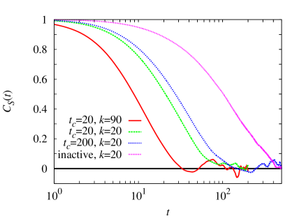
Figure 2: Plot of the orientational correlation function $C_{S}(t)=\langle\cos\theta(t)\rangle$, where $\theta$ is the angle between the dumbbell’s initial orientation and its orientation at time $t$, against $t$ for a single dumbbell in solution. Parameters are indicated in the legend.

The force dipole for a dumbbell molecule is $m(t)=-k_{0}\ell(t)(\ell(t)-\ell_{0})$, where $k_{0}$ and $\ell_{0}$ stand for, respectively, the spring constant and bond rest length at the time when $m(t)$ is measured. We define the normalized temporal force-dipole autocorrelation function by $C_{m}(t)=\langle\Delta m(t)\Delta m(0)\rangle/\langle\Delta m^{2}\rangle$, with $\Delta m=m-\langle m\rangle$. It has an initial value of unity and decays to zero at long times, since the asymptotic value of $\langle m(t)m(0)\rangle$ is $\langle m\rangle^{2}$. This correlation function is plotted in Fig. 3(a) for several values of the force constant $k$. The force dipole correlations decay with a strongly damped oscillatory tail at longer times that is due to the changes in sign when the forces that trigger closing or opening change their sign. The force dipole correlation time $t_{m}$, defined as the time for $C_{m}(t)$ to decay to 1/e of its initial value, ranges from $t_{m}\approx 2-7$ for the data in the figure. These times are less than an order of magnitude shorter than the orientational correlation times. For active dumbbells $\langle\Delta m^{2}\rangle$ depends on $k$, $\ell_{o,c}$ and $t_{c}$, and its magnitude decreases with increasing $t_{c}$. We find that it scales with the force constant as $\langle\Delta m^{2}\rangle\sim k^{\alpha}$, where $\alpha$ also changes with $t_{c}$. For the results shown in the inset to Fig. 3(a), we find $\alpha\sim 1.6$ for $t_{c}=20$ and $\alpha\sim 1.2$ for $t_{c}=100$. In the limit $t_{c}\to\infty$, $\alpha=1$.

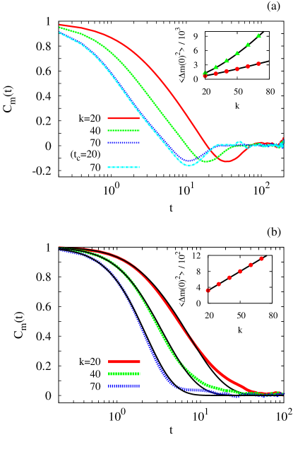
Figure 3: (a) Plot of $C_{m}(t)=\langle\Delta m(t)\Delta m(0)\rangle/\langle\Delta m^{2}\rangle$, with $m=-k_{0}\ell(\ell-\ell_{0})$ the force dipole for a dumbbell, against $t$ for an active dumbbell with $t_{c}=100$. The value of $k$ is indicated in the legend. Also shown is data for $t_{c}=20$ at $k=70$. The value of $\langle\Delta m^{2}\rangle$ is plotted in the inset as a function of $k$ for $t_{c}=100$ (red circles) and $t_{c}=20$ (green triangles). The solid lines show the dependence of this quantity on $k^{\alpha}$ with $\alpha$ indicated in the plot. (b) Plot of $C_{m}(t)$ against $t$ for an inactive dumbbell. Solid black lines show the theoretical prediction given by Eq. (III). The value of $\langle\Delta m^{2}\rangle$ is shown in the inset as a function of $k$, where the solid line shows a $k^{\alpha}$ dependence with $\alpha=1$.

The results for an active dumbbell may be contrasted with those for an inactive dumbbell that simply experiences thermal fluctuations about its open conformation. The correlation function $C_{m}(t)$ for this situation is plotted in Fig. 3(b). It decays monotonically to its long-time value, signalling the absence of anti-correlation effects that arise from the active dumbbell conformational changes. In addition, $\langle\Delta m^{2}\rangle$ now scales as $\langle\Delta m^{2}\rangle\sim k$.

A simple Langevin model,

$$\mu\frac{d^{2}\ell(t)}{dt^{2}}=-\zeta\frac{d\ell(t)}{dt}-\mu\omega_{o}^{2}(\ell(t)-\ell_{o})+f(t),$$ (4)

can be used to compute $C_{m}(t)$ for an inactive dumbbell. In this equation $\zeta$ is the friction coefficient, $\mu=m_{b}/2$ is the relative dumbbell mass, $\omega_{o}^{2}=k_{o}/\mu$ and $f(t)$ is a Gaussian white-noise random force with correlation function $\langle f(t)f\rangle=2k_{B}T\zeta\delta(t)$. The force dipole here takes the form $m(t)=-k_{o}\ell(t)(\ell(t)-\ell_{o})$ with $k_{o}=k$. Using the solution of Eq. (4), the unnormalized force dipole correlation function is given by

$$\langle m(t)m(0)\rangle=(k_{B}T)^{2}\Big{\{}1+$$

$$2e^{-\gamma t}\big{(}1+\big{(}2+\big{(}\frac{\omega_{o}}{\omega}\big{)}^{2}\big{)}\sinh^{2}\omega t+\frac{\gamma}{2\omega}\sinh 2\omega t\big{)}+$$

$$\frac{k\ell_{o}^{2}}{k_{B}T}e^{-\gamma t/2}\big{(}\frac{\gamma}{2\omega}\sinh\omega t+\cosh\omega t\big{)}\Big{\}},$$ (5)

where $\gamma=\zeta/\mu$, $\omega=\sqrt{\gamma^{2}/4-\omega_{o}^{2}}$ with $\gamma>2\omega_{o}$ for overdamped dynamics. Its limiting form is $\lim_{t\to\infty}\langle m(t)m(0)\rangle=\langle m\rangle^{2}=(k_{B}T)^{2}$, which we may use to calculate $C_{m}(t)$. The only unknown parameter in the expression for $\langle m(t)m(0)\rangle$ is the friction coefficient $\zeta$ that appears in the ratio $\gamma=\zeta/\mu$. By fitting to the data for a single force constant, we obtain a value of $\gamma\sim 3.19$, from which one obtains good agreement with the simulation results for all values of the force constant shown in Fig. 3(b). In the strongly overdamped limit Eq. (III) takes the simpler form,

$$\langle m(t)m(0)\rangle=(k_{B}T)^{2}\Big{\{}1+2e^{-2kt/\zeta}+\frac{k\ell_{o}^{2}}{k_{B}T}e^{-kt/\zeta}\Big{\}}.$$ (6)

For inactive dumbbells $\langle\Delta m^{2}\rangle=(k_{B}T)^{2}\left(2+k\ell_{o}^{2}/k_{B}T\right)$, which shows the linear scaling of $\langle\Delta m^{2}\rangle$ with $k$ seen in the inset to Fig. 3(b). Since $k\ell_{o}^{2}/2k_{B}T\gg 1$, to a good approximation we may write $\langle m^{2}\rangle/k\ell_{o}^{2}\approx k_{B}T$ and this ratio is approximately independent of the force constant magnitude. The decay from this initial value of $C_{m}(t)$ depends on the value of the $k$, with a larger value resulting in a faster decay, as can be seen in Fig. 3(b). The decay time $t_{m}$ varies between $t_{m}\approx 2-8$, comparable to that for active dumbbells, albeit from a smaller initial value.

IV Diffusion in a field of active dumbbells

The diffusion of a passive particle as well as the self-diffusion of an active dumbbell, in a field of active dumbbell molecules, are discussed in this section. A visual representation of the system under study is given in Fig. 4, which shows an instantaneous configuration of the dumbbells and passive particle drawn from the dynamics. Solvent particles are not displayed due to their large number.

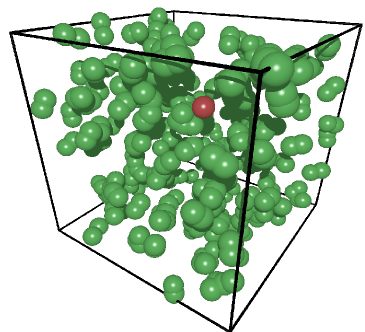
Figure 4: Instantaneous configuration of the system showing active dumbbells (green) and the single passive particle (red) for a system with dumbbell volume fraction $\phi=0.133$.

All our simulations start from an isotropic configuration of dumbbell particles, and for all the system parameters studied here we find no evidence of positional or orientational ordering of the dumbbells.

Passive particle diffusion

As briefly described in the Introduction, the diffusion coefficients of passive particles are enhanced when the medium in which they move contains active enzymes or swimmers. Recent experimental studies have shown that even on microscopic scales the diffusion of passive molecular tracers are enhanced in the presence of active catalyst molecules. Dey et al. (2016) In this subsection, we determine how the diffusion coefficient of a passive tracer particle varies as a function of the volume fraction of active dumbbells. Although our study is motivated by the diffusive dynamics of active enzyme systems, no specific enzymatic system is considered. Rather, we explore the dependence of the diffusion coefficients on a wide range of dumbbell and other system parameters.

Consider a single passive particle immersed in a system of volume $V$ containing $n_{\mathrm{db}}$ dumbbells with volume fraction $\phi=v_{\mathrm{db}}n_{\mathrm{db}}/V=v_{\mathrm{db}}c$, where $v_{\mathrm{db}}$ is the volume of a dumbbell and $c=n_{\mathrm{db}}/V$ is the dumbbell concentration. We define this volume to be that of overlapping monomer spheres with radius $\sigma_{c}/2$ in the open configuration, $v_{\mathrm{db}}=2\pi[\sigma^{3}_{c}/2-(\sigma_{c}-l_{o})^{2}(2\sigma_{c}+l_{o})/8]/3$ with $v_{\mathrm{db}}=82.96$ for the parameters used here. The effective volume will also vary as the dumbbell undergoes conformational changes, so the volume fraction obtained using this value of $v_{\mathrm{db}}$ simply provides a convenient way to specify the dumbbell concentration, $c$.

The diffusion coefficient $D$ may be determined from the long-time limit of the mean square displacement  $\Delta R^{2}(t)=\langle|{\bf R}(t)-{\bf R}(0)|^{2}\rangle\sim 6Dt$, where ${\bf R}$ is the position of the passive particle and the angular brackets denote a time and ensemble average. In general the diffusion coefficient will depend on the dumbbell volume fraction, force constants and average hold time, $D=D(\phi,k,t_{c})$. In the absence of dumbbells ($\phi=0$) it will be denoted by $D_{0}$ and for our system parameters this has the value $D_{0}=1.14\times 10^{-3}$. The thermal diffusion coefficient of the passive particle in a solution containing inactive dumbbells, denoted by $D_{T}(\phi)$, will also be a function of the dumbbell volume fraction, since crowding by dumbbells will alter its value.

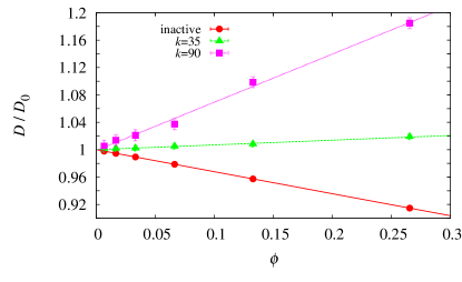
Figure 5: Diffusion coefficient $D$ of the passive particle versus dumbbell volume fraction $\phi$, in a system of active dumbbells with $t_{c}=20$ and two values of the force constant $k$ indicated in the figure. Also shown is $D_{T}$, the diffusion coefficient of a passive particle in a system of inactive dumbbells. Data is normalized by $D_{0}$, the diffusion coefficient of a single passive particle in the absence of dumbbells.

Figure 5 compares the dependence of $D$, for two values of $k$ and fixed $t_{c}=20$, and $D_{T}$ on $\phi$. (Additional data is given in the Appendix B.) For inactive dumbbells $D_{T}(\phi)$ decreases with increasing $\phi$, consistent with the fact that the inactive dumbbells act as crowding agents and inhibit the diffusive dynamics of the passive particle. The solid line in the figure shows that the diffusion coefficient varies linearly with $\phi$ over the range of volume fractions presented. Expressed as a function of $\phi$, we have $D_{T}(\phi)=D_{0}(1+\kappa_{o}\phi)$, where the constant $\kappa_{o}=-0.321$, which is independent of $k$, is obtained from a fit to the data. The dependence on the dumbbell volume fraction is different when the dumbbells are active: now $D$ increases with increasing $\phi$ over the same range of $\phi$ values, rather than decreasing as is the case for crowding by inactive dumbbells. We may write $D(\phi,k,t_{c})=D_{0}(1+\kappa(k,t_{c})\phi)$, where $\kappa$ depends on $k$ and $t_{c}$, with $\kappa=0.701$ and 0.067 for $k=90$ and $35$, respectively, for the data in Fig. 5.

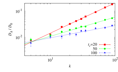
Figure 6: Active contribution to the diffusion coefficient, $D_{A}/D_{0}$, as a function of $k$ for several values of $t_{c}$ and $\phi=0.133$. Points show simulation data, lines show fits of the form $D_{A}/D_{0}=\lambda k^{\delta}\phi$ to the data.

The active contribution to the diffusion coefficient, $D_{A}$, is defined by the equation $D=D_{T}+D_{A}$. Extensive computations of $D_{A}(\phi,k,t_{c})$ have been carried out to determine its dependence on the dumbbell volume fraction, force constant and average hold time. Figure 6 shows that for fixed $\phi$, $D_{A}$ has a power-law dependence on $k$ of the form $D_{A}\sim k^{\delta}$, where the exponent $\delta$ depends on $t_{c}$. For a fixed value of $k$, as $t_{c}$ increases $D_{A}$ decreases. The larger $t_{c}$ is, the slower $D_{A}$ increases with $k$. The results of these simulations may be summarized in the following form for the diffusion coefficient:

$$D(\phi,k,t_{c})=D_{T}(\phi)+D_{0}\kappa_{A}(k,t_{c})\phi,$$ (7)

where $\kappa_{A}(k,t_{c})=\kappa(k,t_{c})-\kappa_{o}=\lambda(t_{c})k^{\delta(t_{c})}$. Additional information on the dependence of $\lambda$ and $\delta$ on $t_{c}$ is given in Appendix B. These results are applicable provided $k$ is not too small since as $k\to 0$ the dumbbell bond will soften and the dumbbell will dissociate. Note that as $t_{c}\to\infty$ we have $\kappa(k,t_{c})\to\kappa_{c}$, its value for a dumbbell that fluctuates about its closed conformation.

Depending on the system parameters, it is possible that the decrease in diffusion due to crowding-induced hindered motion may be larger than the increase due to dumbbell activity. In such a circumstance $D(\phi)/D_{0}$ may be less than unity ($\kappa(k,t_{c})<0$), although the ratio will be larger than $D_{T}(\phi)/D_{0}$ for systems with inactive dumbbells. In our simulations we found that $\kappa(k,t_{c})>0$ for most values of $k$ and $t_{c}$, although for a given $t_{c}$ there is a $k$ value at which $\kappa(k,t_{c})$ will change sign. This will occur when $\kappa(k,t_{c})=0$, which corresponds to $k=(-\kappa_{o}/\lambda(t_{c}))^{1/\delta(t_{c})}$, given the scaling forms below Eq. (7).

The magnitude of the enhancement of the diffusion coefficient as measured by $D_{A}/D_{T}$ depends strongly on the system parameters, $\phi$, $k$ and $t_{c}$, as well as $\tau_{{\text{M}PC}}$, which determines the solvent properties. The largest enhancements for $k=90$, $t_{c}=20$, $\tau_{{\text{M}PC}}=0.01$ in Fig. 5 are $D_{A}/D_{T}\approx 0.15$ and $D_{A}/D_{T}\approx 0.3$ for $\phi=0.133$ and $0.266$, respectively. For another set of system parameters with $\tau_{{\text{M}PC}}=0.05$, corresponding to a smaller solvent viscosity, $t_{c}=20$ and $k=9$, we find $D=4.68\times 10^{-3}$ and $D_{0}=4.44\times 10^{-3}$ for $\phi=0.133$ giving $D_{A}/D_{T}\approx 0.05$. In addition to the quantitative estimates of the diffusion enhancement, several qualitative features of $D_{A}$ are worth summarizing. The coefficient $\kappa_{A}$ differs from $\kappa_{o}$ since it depends strongly on $k$ and $t_{c}$. For fixed $t_{c}$, $\kappa_{A}\sim k^{\delta}$ where the exponent $\delta$ decreases with increasing $t_{c}$. These qualitative features of $D_{A}$ differ markedly from those that characterize the behavior of $D_{T}$.

Active contributions to passive particle diffusion from the collective hydrodynamic interactions of many active proteins were discussed earlier using a Langevin model. Mikhailov and Kapral (2015) The result was the following estimate for $D_{A}$:

$$D_{A}^{\text{th}}=\frac{S_{A}}{60\pi\ell_{{\text{c}ut}}\eta^{2}v_{\mathrm{ex}}}\phi\equiv D_{0}\kappa_{A}^{\text{th}}(k,t_{c})\phi,$$ (8)

for a uniform distribution of proteins with concentration $c=\phi/v_{\mathrm{ex}}$. This order-of-magnitude estimate was derived assuming a random static distribution of protein orientations, slow protein translational dynamics, and Oseen interactions with a short-distance cut-off, $\ell_{{\text{c}ut}}$, taken to be the sum of the effective radii of the passive particle and protein. In this equation $S_{A}$ characterizes the strength of the force dipole correlations, $\langle\Delta m(t)\Delta m(0)\rangle$. The last equality defines the theoretical estimate of $\kappa_{A}$. Evaluation of Eq. (8) for a range of $k$ and $t_{c}$ values shows that $\kappa_{A}^{\text{th}}(k,t_{c})\sim k^{\sigma}$ for fixed $t_{c}$, where $\sigma<\delta$, smaller than the exponent $\delta$ found from simulation. The predicted values of the diffusion enhancement are consistent with Eq. (8) since they differ by less than an order-of-magnitude from those in our microscopic simulations; for example, for $\phi=0.133$, $k=35$ and $t_{c}=20$ we have $D_{A}^{\text{th}}/D_{T}=0.01$ while from simulation $D_{A}/D_{T}=0.051$.

Active dumbbell self-diffusion

The self-diffusion coefficients of the dumbbells themselves, $D_{\mathrm{db}}$, are also modified due to crowding by other dumbbells, and the effects of crowding differ depending on whether the dumbbells are active or inactive. Figure 7(a) shows $D_{\mathrm{db}}^{T}$ and $D_{\mathrm{db}}$, the diffusion coefficients for inactive and active dumbbells, respectively, as a function of $\phi$, normalized by the diffusion coefficient of a single inactive dumbbell, $D_{\mathrm{db}}^{0}=1.625\times 10^{-3}$. For inactive dumbbells $D_{\mathrm{db}}^{T}$ decreases with increasing $\phi$, as expected for a crowded environment. A similar trend is seen for active dumbbells, with $D_{\mathrm{db}}$ also decreasing with an increase in $\phi$, although the decrease is much smaller than that for inactive dumbbells. As discussed above, recall that even for the passive particle in a system of active dumbbells, depending on the system parameters, the diffusion coefficient $D$ may decrease as $\phi$ is increased, but this decrease will be less strong than that for a system of inactive dumbbells. In these cases the effects of activity are not sufficient to completely overcome the tendency for crowding to decrease the diffusion coefficient. Nevertheless, $D_{\mathrm{db}}/D_{\mathrm{db}}^{T}>1$ and the magnitudes of the diffusion coefficient changes are comparable to those for the passive particle. For example, for a volume fraction of $\phi=0.133$ and $k=90$, $t_{c}=20$, $\tau_{{\text{M}PC}}=0.01$ we have $D_{\mathrm{db}}/D_{\mathrm{db}}^{T}\approx 1.19$, while for $k=9$, $t_{c}=20$, $\tau_{{\text{M}PC}}=0.05$ we have $D_{\mathrm{db}}/D_{{\text{d}b}}^{T}\approx 1.05$.

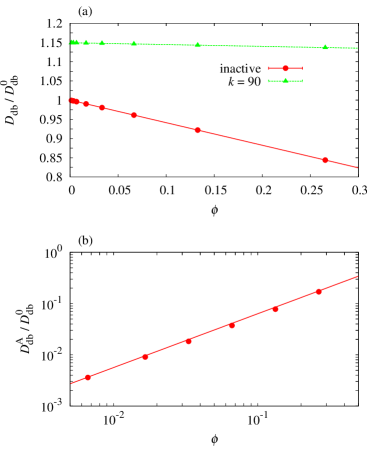
Figure 7: (a) Dumbbell self-diffusion coefficient $D_{\mathrm{db}}$ versus $\phi$, for a system of active dumbbells with $t_{c}=20$ and $k=90$ (green triangles), and $D_{\mathrm{db}}^{T}$ for a system of inactive dumbbells (red circles). Data is normalized by $D_{\mathrm{db}}^{0}$, the diffusion coefficient of a single inactive dumbbell. (b) Active contribution to the dumbbell self-diffusion coefficient $D^{A}_{\mathrm{db}}$ versus $\phi$.

Although the tendency for $D_{\mathrm{db}}$ to increases or decrease with increasing $\phi$ depends on the system parameters, one can see that the values of the dumbbell self-diffusion coefficients differ markedly depending on whether they are active or inactive. In contrast to $D$ for passive particle diffusion, which tends to a common value of $D_{0}$ as $\phi\to 0$ regardless of whether the dumbbells are active or inactive, even for a single dumbbell in solution $D_{\mathrm{db}}$ will be different if it is active or inactive. For example, for the data in Fig. 7(a), $D_{\mathrm{db}}(\phi=0)=2.0\times 10^{-3}$ and $D_{{\text{d}b}}/D_{\mathrm{db}}^{0}\approx 1.15$ for a single dumbbell in solution. Since $D_{\mathrm{db}}$ depends on the dumbbell conformation and is larger when the dumbbell is in the compact closed form, one expects, and finds, $D_{\mathrm{db}}>D_{{\text{d}b}}^{T}$. [Suchdependenceofdiffusiononconformationaldynamicswasobservedearlierinaninvestigationofactiveenzymedynamicsforadenylatekinase(AKE).Theenzymecatalyzesthereversiblereaction$AMP+ATP⇌2ADP$andintheprocesschangesitsconformationandcyclesfromopentoclosedforms.Thediffusioncoefficientforthecatalyticallyactiveenzymewasfoundtobelargerthatfortheenzymeisinitsopenconformationwhennosubstrateisbound; $D_\text{A}KE/D^T_\text{A}KE≈1.17$; similartotheresultsforthedumbbellmodelconsideredhere.]carlos2011 Furthermore, when the average hold time $t_{c}$ is smaller, $D_{\mathrm{db}}(\phi=0)$ becomes smaller, as the dumbbell spends less time in its closed conformation. This results in a measured $D_{\mathrm{db}}$ that is smaller at low $k$ values for dumbbells with shorter average hold times than for ones with larger $t_{c}$ values, as can be seen in Table 3 in Appendix B.

Accounting for the fact that $D_{\mathrm{db}}$ is different for single active and inactive dumbbells in solution, we define the active dumbbell contribution to the self-diffusion coefficient by the equation, $D_{\mathrm{db}}=D^{T}_{\mathrm{db}}+D^{A}_{{\text{d}b}}+D^{A,0}_{\mathrm{db}}$, where $D^{A,0}_{\mathrm{db}}=D_{\text{ db}}(\phi=0)-D^{0}_{\mathrm{db}}$. Figure 7(b) plots $D^{A}_{\mathrm{db}}$ versus $\phi$ and shows that the active contribution increases with increasing $\phi$.

The results presented above show that hydrodynamic interactions resulting from nonequilibrium force dipole fluctuations of the dumbbell molecules give rise to enhanced diffusion of both the passive particle and the dumbbells themselves when compared to their values for systems containing only inactive dumbbells. Direct intermolecular interactions also play a role but estimates based on dumbbell sizes and ranges of intermolecular forces suggest that these interactions are important only at the highest volume fractions considered in this study. Contributions from direct intermolecular interactions will increase in importance as the average separation between dumbbells $l_{\mathrm{sep}}=(v_{\mathrm{ex}}/\phi)^{1/3}$ approaches the maximum length of a dumbbell $l_{\mathrm{db}}=\ell_{o}+2\sigma_{c}=8.3$. This is the case only for systems with the largest two volume fractions studied, $\phi=0.133$ and $\phi=0.266$, where $l_{\mathrm{sep}}=8.54$ and $6.78$, respectively.

V Conclusions

The microscopic simulation systems containing a passive particle and either active or passive dumbbell molecules has allowed us to explore how diffusive dynamics varies with dumbbell activity and volume fraction. The results showed that the diffusive dynamics of passive particles in systems crowded by active molecules that change their conformations differs markedly from that when the crowding molecules are inactive. The self-diffusion coefficients of the crowding molecules themselves also display properties that depend on their activity. While crowding by molecules that thermally fluctuate about their open (or closed) metastable states leads to well-known subdiffusive dynamics and diffusion coefficients that decrease with increasing volume fraction, diffusion coefficients are enhanced, or decrease more slowly, when the crowding agents are active.

Hydrodynamic interactions induced by active force dipole fluctuations are responsible for the observed diffusion coefficient increases, and direct intermolecular interactions contribute at the highest volume fractions. The particle-based dynamical model used in this investigation accounts for both of these effects and permits a detailed analysis of the phenomena. The magnitudes of the changes to the diffusion coefficient were shown to depend not only on the volume fraction of dumbbells, but also on the force dipole strength and the mean times spent in the open or closed conformations. The diffusion enhancement in experiments and in our simulations is not large but its existence signals that conformational changes arising from catalytic activity play a role in transport in active systems.

The dumbbell conformational changes in this study were specified by a stochastic model that was chosen to mimic some features of the cyclic dynamics of enzymes undergoing conformational changes during their catalytic operation. Our dynamical model can be generalized to include a more detailed description of the substrate binding, unbinding and reaction processes with the enzyme so that the dependence of the effects on substrate concentration can be investigated. More realistic enzyme models may also be employed. Echeverria et al. (2011); Schofield et al. (2014) The results in this paper provide the basis for the development and further study of more realistic models to probe transport properties in systems crowded by chemically active and inactive molecules and their relevance to biochemical processes in the cell.

Acknowledgements: We would like to thank Alexander Mikhailov for useful discussions on this topic. The research of RK was supported in part by a grant from the Natural Sciences and Engineering Research Council of Canada. MD thanks the Humboldt foundation for financial support. RK and MD were partially supported through the research training group GRK 1558 funded by Deutsche Forschungsgemeinschaft.

Appendix A

Multiparticle collisions were implemented using the MPC-AT+a rule that employs the Anderson thermostat and conserves linear and angular momentum. Noguchi and Gompper (2004); *ref:noguchi2007; *ref:noguchi2007b Allowing the solvent particles to interact and exchange momentum only in the collision step, the frequency of which can be chosen according to the desired properties of the solvent, makes the method computationally efficient. Since the collision rule conserves mass and momentum at the cell level, the hydrodynamic flow fields will be described correctly, a feature that is essential for hydrodynamic interactions. The solvent viscosity $\eta$ can be controlled by varying the number of solvent particles $n_{f}$ per collision cell and/or the MPC time, $\tau_{{\text{M}PC}}$. Kapral (2008); Gompper et al. (2009) In our simulations, we use a cubic simulation box of linear size $n_{x}=50$ MPCD cells in each direction, with $n_{f}=10$ fluid particles per cell, and an MD time step of $\Delta t=0.001$.

The choice of parameters was based on several criteria. We wish to study a large range of force constants in order to identify the underlying trends in the system behaviour. Since inertia does not play a significant role in protein dynamics in solution, the dumbbell dynamics should be overdamped. This condition sets a limit on the maximum value of the spring constant. Furthermore, for spring energies which are comparable to the thermal energy ($k\sim k_{B}T/a^{2}$), thermal fluctuations dominate the dumbbell motion. This lower bound depends only on the value of $k_{B}T$, and not on any other fluid parameters. We consider two values of the MPC time, $\tau_{{\text{M}PC}}=0.01$ which gives a large fluid viscosity of $\eta\sim 36$, and $\tau_{{\text{M}PC}}=0.05$ which gives a lower fluid viscosity of $\eta\sim 8.4$. In simulations with the higher viscosity a large range of force constant values may be used while still remaining in the regime of overdamped dynamics.

The dumbbell mass is chosen so that it is neutrally buoyant. Since the dumbbell interacts with the solvent only in the MPC collision step, we define the volume of interaction of a dumbbell with the fluid by $v_{\mathrm{f,db}}=4\pi r_{\mathrm{f,db}}^{3}/3$, where $r_{\mathrm{f,db}}=(\ell_{o}+\ell_{c})/2$, which corresponds to a sphere with a diameter equal to the average dumbbell spring rest length. Note that this is distinct from the dumbbell volume $v_{\mathrm{db}}$ defined earlier. This then gives a total dumbbell mass of $m_{\mathrm{db}}=v_{\mathrm{f,db}}n_{f}$. Throughout we set $\ell_{c}=2$ and $\ell_{o}=4$, such that we have $m_{\mathrm{db}}=141.37$. From our fluid and dumbbell parameters we then obtain a cross-over spring constant between overdamped and underdamped motion of $k_{o}>90$ for $\tau_{{\text{M}PC}}=0.01$ and $k_{o}>11$ for $\tau_{{\text{M}PC}}=0.05$.

To control the switching between the two spring rest lengths we must set the cut-off parameter that the length must cross before the hold time is chosen. We set $\delta\ell_{o}=\delta\ell_{c}=0.05(\ell_{o}-\ell_{c})=0.1$. The hold times are chosen from log normal distributions with averages for the open and closed configurations of $t_{o}$ and $t_{c}$, and with scale parameter $\sigma=0.5$. Throughout the time spent in the open configuration is $t_{o}=0$.

For the passive particle we set the passive particle-fluid interaction radius to be $\sigma_{cf}=2$ and the passive particle-dumbbell bead interaction diameter to be $\sigma_{c}=4.30$. The passive particle is also chosen to be neutrally buoyant, such that its mass is given by $m_{c}=4\pi\sigma^{3}_{cf}n_{f}/3$ which for the parameters given here is $m_{c}=335.103$.

Dimensionless units can be mapped approximately onto physical units by matching dimensions and time scales. Padding and Louis (2006) Consider $\tau_{{\text{M}PC}}=0.05$ for which $D_{0}=4.44\times 10^{-3}\;a^{2}/t_{0}$. Taking a radius of 5 nm for the passive particle and assuming $D_{0}$ is given by its Stokes-Einstein value one finds $t_{0}\approx 0.1$ ns. For $k=9\;k_{B}T/a^{2}$ we then have for the forces corresponding to active opening and closing $F\approx 20$ pN.

Appendix B

This Appendix provides some of the numerical values of the data in the plots, along with parameters that enter in the phenomenological forms for the diffusion coefficients. The data used to construct Fig. 5 is in Table 1.

$\phi/10^{-2}$	$k$	$D/10^{-3}$	$D_{T}/10^{-3}$
$0.66$	$90$	$1.145$	$1.137$
$1.66$	$90$	$1.155$	$1.134$
$3.32$	$90$	$1.163$	$1.128$
$6.64$	$90$	$1.182$	$1.115$
$13.3$	$90$	$1.261$	$1.092$
$26.6$	$90$	$1.350$	$1.043$
$0.66$	$35$	$1.140$	$1.137$
$1.66$	$35$	$1.141$	$1.134$
$3.32$	$35$	$1.142$	$1.128$
$6.64$	$35$	$1.145$	$1.115$
$13.3$	$35$	$1.148$	$1.092$
$26.6$	$35$	$1.160$	$1.043$

Table 1: Values of $D$ and $D_{T}$ plotted in Fig. 5 as functions of volume fraction $\phi$ for $t_{c}=20$ and two values of $k$, for systems with $\tau_{{\text{M}PC}}=0.01$.

Table 2 gives representative values of the parameters that enter in Eq. (7) for the passive particle diffusion coefficient.

$\phi/10^{-2}$	$t_{c}$	$\lambda/10^{-3}$	$\delta$	Fit $D_{T}/10^{-3}$	Sim $D_{T}/10^{-3}$
$0.66$	$20$	$5.18$	$1.13$	$1.137$	$1.137$
$1.66$	$20$	$4.74$	$1.12$	$1.133$	$1.134$
$3.32$	$20$	$3.60$	$1.16$	$1.128$	$1.128$
$6.64$	$20$	$4.30$	$1.12$	$1.112$	$1.115$
$13.3$	$20$	$4.74$	$1.16$	$1.086$	$1.092$
$26.6$	$20$	$4.82$	$1.18$	$1.052$	$1.043$
$13.3$	$30$	$11.0$	$0.98$	$1.087$	$1.092$
$13.3$	$50$	$19.5$	$0.73$	$1.083$	$1.092$
$13.3$	$100$	$37.1$	$0.47$	$1.084$	$1.092$
$13.3$	$200$	$78.6$	$0.20$	$1.097$	$1.092$

Table 2: Values of $\lambda$, $\delta$ and $D_{T}$ found from fitting $D=D_{T}+D_{0}\lambda k^{\delta}\phi$ to the data, for systems with $\tau_{{\text{M}PC}}=0.01$, and with volume fraction and average hold time $t_{c}$ indicated. The last column gives $D_{T}$ as measued in a system of inactive dumbbells.

Table 3 presents data for the dumbbell self-diffusion coefficient for several values of the hold time $t_{c}$ and force constant $k$.

$t_{c}$	$k$	$D_{\mathrm{db}}/10^{-3}$
$30$	$5$	$1.707$
$30$	$10$	$1.727$
$30$	$20$	$1.758$
$30$	$35$	$1.783$
$30$	$90$	$1.908$
$50$	$5$	$1.717$
$50$	$10$	$1.729$
$50$	$20$	$1.743$
$50$	$35$	$1.774$
$50$	$90$	$1.847$
$100$	$5$	$1.724$
$100$	$10$	$1.741$
$100$	$20$	$1.753$
$100$	$35$	$1.770$
$100$	$90$	$1.817$
inactive	$90$	$1.625$

Table 3: Diffusion coefficients $D_{\mathrm{db}}$ of dumbbell particles for systems with $\tau_{{\text{M}PC}}=0.01$, at average hold times and with spring constants indicated in the table. All other parameters are set to the values used throughout, given in the text of the paper. Data for both a system of active dumbbells with average hold time $t_{c}$ and a system of inactive dumbbells are presented, all at a volume faction of $\phi=0.133$.

References

- Caspi et al. (2000) A. Caspi, R. Granek, and M. Elbaum, Phys. Rev. Lett. 85, 5655 (2000).
- Lau et al. (2003) A. W. C. Lau, B. D. Holfman, A. Davies, J. C. Crocker, and T. C. Lubensky, Phys. Rev. Lett. 91, 19810 (2003).
- MacKintosh and Levine (2008) F. C. MacKintosh and A. J. Levine, Phys. Rev. Lett. 100, 018104 (2008).
- Wilhelm (2008) C. Wilhelm, Phys. Rev. Lett. 101, 028101 (2008).
- Gallet et al. (2009) F. Gallet, D. Arcizet, P. Bohec, and A. Richert, Soft Matter 5, 2947 (2009).
- Weber et al. (2012) S. C. Weber, A. J. Spakowitz, and J. A. Theriot, PNAS 109, 7338 (2012).
- Bruinsma et al. (2014) R. Bruinsma, A. Y. Grosberg, Y. Rabin, and A. Zidovska, Biophys. J. 106, 1871 (2014).
- Guo et al. (2014) M. Guo, A. J. Erlicher, M. H. Jensen, M. Renz, J. R. Moore, R. D. Goldman, J. Lippincott-Shwartz, F. C. Mackintosh, and D. A. Weitz, Cell 158, 822 (2014).
- Mizuno et al. (2007) D. Mizuno, C. Tardin, C. F. Schmidt, and F. C. MacKintosh, Science 315, 370 (2007).
- Toyota et al. (0011) T. Toyota, D. A. Head, C. F. Schmidt, and D. Mizuno, Soft Matter 7, 3234 (20011).
- Muddana et al. (2010) H. S. Muddana, S. Sengupta, T. E. Mallouk, A. Sen, and P. J. Butler, J. Am. Chem. Soc. 132, 2110 (2010).
- Sengupta et al. (2013) S. Sengupta, K. K. Dey, H. S. Muddana, T. Tabouillot, M. E. Ibele, P. J. Butler, and A. Sen, J. Am. Chem. Soc. 135, 1406 (2013).
- Pavlick et al. (2013) R. A. Pavlick, K. K. Dey, A. Sirjoosingh, A. Benesi, and A. Sen, Nanoscale 5, 1301 (2013).
- Golestanian (2015) R. Golestanian, Phys. Rev. Lett. 115, 108102 (2015).
- Mikhailov and Kapral (2015) A. M. Mikhailov and R. Kapral, Proc. Nat. Acad. Sci. USA 112, E3639 (2015).
- Kapral and Mikhailov (2016) R. Kapral and A. M. Mikhailov, Physica D 318-319, 100 (2016).
- Koyano et al. (2016) Y. Koyano, H. Kitahata, and A. S. Mikhailov, Phys. Rev. E 94, 022416 (2016).
- Kim and Breuer (2004) M. J. Kim and K. Breuer, Phys. Fluids 16, L78 (2004).
- Leptos et al. (2009) K. C. Leptos, J. S. Guasto, J. P. Gollub, A. I. Pesci, and R. E. Goldstein, Phys. Rev. Lett. 103, 198103 (2009).
- Mino et al. (2013) G. L. Mino, J. Dunstan, A. Rousselet, E. Clement, and R. Soto, J. Fluid Mech. 729, 423 (2013).
- Saintillan and Shelley (2012) D. Saintillan and M. J. Shelley, J. R. Soc. Interface 9, 571 (2012).
- Kasyap et al. (2014) T. V. Kasyap, D. L. Koch, and M. Wu, Phys. Fluids 26, 081901 (2014).
- Metzler and Klafter (2000) R. Metzler and J. Klafter, Phys. Repts. 339, 1 (2000).
- Schnell and Turner (2004) S. Schnell and T. E. Turner, Biophys. Mol. Bio. 85, 235 (2004).
- Höfling and Franosch (2013) F. Höfling and T. Franosch, Rep.Prog. Phys. 76, 046602 (2013).
- Nakano et al. (2014) S. Nakano, D. Miyoshi, and N. Sugimoto, Chem. Rev. 114, 2733 (2014).
- Kuznetsova et al. (2014) I. M. Kuznetsova, K. K. Turoverov, and V. N. Uversky, Int. J. Mol. Sci. 15, 23090 (2014).
- Padding and Louis (2006) J. T. Padding and A. A. Louis, Phys. Rev. E 74, 031402 (2006).
- Malevanets and Kapral (1999) A. Malevanets and R. Kapral, J. Chem. Phys. 110, 8605 (1999).
- Malevanets and Kapral (2000) A. Malevanets and R. Kapral, J. Chem. Phys. 112, 7260 (2000).
- Kapral (2008) R. Kapral, Adv. Chem. Phys. 140, 89 (2008).
- Gompper et al. (2009) G. Gompper, T. Ihle, D. M. Kroll, and R. G. Winkler, Adv. Polym. Sci. 221, 1 (2009).
- Mussawisade et al. (2005) K. Mussawisade, M. Ripoll, R. G. Winkler, and G. Gompper, J. Chem. Phys. 123, 144905 (2005).
- Ripoll et al. (2006) M. Ripoll, R. G. Winkler, and G. Gompper, Phys. Rev. Lett. 96, 188302 (2006).
- Kogler (2012) F. Kogler, Master’s thesis: Interactions of artificial molecular machines (Technical University of Berlin, 2012).
- Dey et al. (2016) K. K. Dey, F. Y. Pong, J. Breffke, R. Pavlick, E. Hatzakis, C. Pacheco, and A. Sen, Angew. Chem. Int. Ed. 55, 1113 (2016).
- Note (1) As the volume fraction increases the mean square displacement will generally exhibit subdiffusive dynamics on intermediate time scales. Here we focus on the diffusion coefficient determined in the long-time regime where normal diffusion again observed.
- Echeverria et al. (2011) C. Echeverria, Y. Togashi, A. S. Mikhailov, and R. Kapral, Phys. Chem. Chem. Phys 13, 10527 (2011).
- Schofield et al. (2014) J. M. Schofield, P. Inder, and R. Kapral, J.. Chem. Phys 136, 205101 (2014).
- Noguchi and Gompper (2004) H. Noguchi and G. Gompper, Phys. Rev. Lett. 93, 258102 (2004).
- Noguchi et al. (2007) N. Noguchi, N. Kikuchi, and G. Gompper, Europhys. Lett. 78, 10005 (2007).
- Götze et al. (2007) I. O. Götze, H. Noguchi, and G. Gompper, Phys. Rev. E 76, 046705 (2007).