HABILITATION à DIRIGER DES RECHERCHES Présentée par Benjamin Lévêque
Generalization of Schnyder woods to orientable surfaces and applications
Soutenue le 19 octobre 2016, devant le jury composé de :
Vincent Beffara Directeur de recherche CNRS, Examinateur Nadia Brauner Professeur, Université Grenoble Alpes, Examinatrice Victor Chepoi Professeur, Université Aix-Marseille, Examinateur Éric Colin de Verdière Directeur de recherche CNRS, Examinateur Stefan Felsner Professeur, TU Berlin, Rapporteur Marc Noy Professeur, UPC Barcelone, Rapporteur Gilles Schaeffer Directeur de recherche CNRS, Rapporteur András Sebő Directeur de recherche CNRS, Examinateur    

Abstract : Schnyder woods are particularly elegant combinatorial structures with numerous applications concerning planar triangulations and more generally 3-connected planar maps. We propose a simple generalization of Schnyder woods from the plane to maps on orientable surfaces of any genus with a special emphasis on the toroidal case. We provide a natural partition of the set of Schnyder woods of a given map into distributive lattices depending on the surface homology. In the toroidal case we show the existence of particular Schnyder woods with some global properties that are useful for optimal encoding or graph drawing purpose.

Keywords : Embedded graphs, Orientable surfaces, Toroidal triangulations, 3-connected maps, $\alpha$-orientations, Schnyder woods, Distributive lattices, Homology, Bijective encoding, Graph drawing

Introduction

Schnyder woods (see Part I) are today one of the main tools in the area of planar graph representations. Among their most prominent applications are the following: They provide a machinery to construct space-efficient straight-line drawings [51, 37, 21], yield a characterization of planar graphs via the dimension of their vertex-edge incidence poset [50, 21], and are used to encode triangulations [45, 4]. Further applications lie in enumeration [10], representation by geometric objects [29, 33], graph spanners [12], etc.

We propose a simple generalization of Schnyder woods from the plane to maps on orientable surfaces of any genus (see Part II). This is done in the language of angle labellings. Generalizing results of De Fraysseix and Ossona de Mendez [30], and Felsner [23], we establish a correspondence between these labellings and orientations and characterize the set of orientations of a map that corresponds to such a Schnyder wood. Furthermore, we study the set of orientations of a given map and provide a natural partition into distributive lattices depending on the surface homology. This generalizes earlier results of Felsner [23] and Ossona de Mendez [44]. Whereas many questions remain open for the double torus and higher genus (like already the question of existence of the studied objects), in the toroidal case we are able to push our study quite far.

The torus can serve as a model for planar periodic surfaces and is for instance often used in statistical physics context since it enables to avoid dealing with particular boundary conditions. It is in a sense the most homogeneous oriented surface since Euler’s formula sums exactly to zero. For our purpose this means that one can asks for orientations satisfying the same local condition everywhere.

We study structural properties of toroidal Schnyder woods extensively (see Part III). We analyze the behavior of the monochromatic cycles of a toroidal Schnyder wood to define the notion of “crossing” that is useful for graph drawing purpose. We also exhibit a kind of “balanced” property that enables to define a canonical lattice and thus a unique minimal element, used in bijections.

We are able to provide several proofs of existence of Schnyder woods in the toroidal case (see Part IV) and this is particularly interesting since this problem is open in higher genus. Some consequences are a linear time algorithm to compute either a crossing Schnyder wood or a minimal balanced Schnyder wood for toroidal triangulations, and the fact that a toroidal map admits a Schnyder wood if and only if it is “essentially 3-connected”.

Concerning the applications (see Part V), we generalize a method devised by Poulalhon and Schaeffer [45] to linearly encode a planar triangulation optimally. In the plane, this leads to a bijection between planar triangulations and some particular trees. For the torus we obtain a similar bijection but with particular unicellular maps (maps with only one face). We also show that toroidal Schnyder woods can be used to embed the universal cover of an essentially 3-connected toroidal map on an infinite and periodic orthogonal surface. We use this embedding to obtain a straight-line flat torus representation of any toroidal map in a polynomial size grid.

Most of the results presented in this manuscript appear in the papers [17, 35, 36]. The goal of this manuscript is to merge these papers and to present them in a unified way. After the first paper [35] our view on the objects have evolved, the definitions have been generalized, enabling to reveal more structural properties. Thus we feel that there was a need to restructure this research in a unique document that also contains additional details, results, corrections and simplifications.

As briefly explained in the conclusion, many of the structural properties that we exhibit here for Schnyder woods can be generalized for other kind of orientations/maps, like transversal structure for 4-connected triangulations, 2-orientations for quadrangulations or more generally $\frac{d}{d-2}$-orientations for d-angulations, etc. There are also probable other applications of Schnyder woods in the plane that can be extended to higher genus. For example we now have all the ingredients to obtain a random generator for toroidal triangulations. For these reasons we believe that this manuscript is just the beginning of more research to come and we hope that it can serve as a starting point for one interested in studying orientations of maps in higher genus and their applications.

I was happy to work on this topic for the last few years and I would like to thank my colleagues, Nicolas Bonichon, Luca Castelli Aleardi and Eric Fusy, whose fruitful discussions have allowed this work to be achieved and also my co-authors, Vincent Despré, Daniel Gonçalves and Kolja Knauer, who have been following me on this journey. We were mostly guided by the beauty of the structural properties of the studied objects, and the nice applications in the end were then just consequences of this quest.

Part I Planar case

Chapter 1 From planar triangulations to Schnyder woods

Before giving the formal definition of Schnyder woods in the plane (see Section 2), we explain how they appear quite naturally while studying planar triangulations.

Given a general graph $G$, let $n$ be the number of vertices and $m$ the number of edges. If the graph is embedded on the plane (or a surface), let $f$ be the number of faces (including the outer face). Euler’s formula says that a connected graph embedded on the plane satisfies $n-m+f=2$.

A general graph (i.e. not embedded on a surface) is simple if it contains no loop and no multiple edges. We start this manuscript with the study of planar triangulations, that are simple graphs embedded in the plane such that every face, including the outer face, has size three (see example of Figure 1.1).

Figure 1.1: Example of a planar triangulation.

Consider a planar triangulation $G$. Since every face has size $3$, we have $3f=2m$. Then by Euler’s formula we obtain $m=3n-6$. Thus there is “almost” $3$ times more edges that vertices in a planar triangulation. In fact, the relation can be re-written $(m-3)=3(n-3)$ so there is exactly three times more internal edges than internal vertices. Thus there is hope to be able to assign to each internal vertex of $G$, three incident edges such that each internal edge is assigned exactly once. By orienting the edges from the vertices to which they are assigned, one obtain an orientation of the graph $G$ where every inner vertex has outdegree exactly $3$ (see Figure 1.2). Such an orientation is called a $3$-orientation.

Figure 1.2: Every inner vertex has outdegree exactly $3$.

Consider a $3$-orientation of $G$. First note that since $(m-3)=3(n-3)$, all the inner edges incident to outer vertices are entering the outer vertices.

Some natural objects to consider in a $3$-orientation are “middle walks”. For an internal edge $e$ of $G$, we define the middle walk from $e$ as the sequence of edges $(e_{i})_{i\geq 0}$ obtained by the following method. Let $e_{0}=e$. If the edge $e_{i}$ is entering an internal vertex $v$, then the edge $e_{i+1}$ is chosen in the three edges leaving $v$ as the edge in the “middle” coming from $e_{i}$ (i.e. $v$ should have exactly one edge leaving on the left of the path consisting of the two edges $e_{i},e_{i+1}$ and thus exactly one edge leaving on the right). If the edge $e_{i}$ is entering an outer vertex, then the walk ends there.

These middles walks have interesting structural properties. First, one can show that a middle walk cannot intersect itself, otherwise it would form a cycle whose interior region would contradicts Euler’s formula by a counting argument (triangulation and 3-orientation inside + middle walk on the border). Thus a middle walk is in fact a middle path and has to end on one of the three outer vertices since it is not infinite.

Let $x_{0},x_{1},x_{2}$ be the three vertices appearing on the outer face in counterclockwise order. One can assign to each inner edge $e$ the color $i\in\{0,1,2\}$ if the middle path starting from $e$ ends at vertex $x_{i}$ (see Figure 1.3). Note that a subwalk of a middle path is also a middle path. So if $e^{\prime}$ is an edge of a middle path then $e$ and $e^{\prime}$ receive the same color. Thus all the edges of a middle path have the same color.

Figure 1.3: All the edges of a middle path are ending at the same outer vertex by following middle edges.

Moreover, consider two distinct outgoing edges $e,e^{\prime}$ of a inner vertex and the two middle paths $W$ and $W^{\prime}$ starting from $e$ and $e^{\prime}$. With similar counting arguments as before, one can show that $W$ and $W^{\prime}$ do not intersect. Thus each of the three middle paths starting from the three outgoing edges of an inner vertex, ends at a different outer vertex. So every vertex has exactly one edge leaving in color $0$, $1$, $2$, respectively, and these edges appear in counterclockwise order (see Figure 1.4).

Figure 1.4: Every inner vertex has exactly one edge leaving in each color.

By the middle path property every edge entering a vertex in color $i$ has to enter in the sector between the outgoing edges of color $i+1$ and $i-1$ (throughout the manuscript colors are given modulo 3). So the inner vertices are satisfying the local property of Figure 1.5 where the depicted correspondence between red, blue, green, 0, 1, 2, and the arrow shapes is used through the entire manuscript.

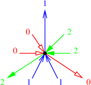
Figure 1.5: Local property satisfied at every inner vertex.

For each color $i$, every inner vertex is the starting point of a middle path of color $i$. This path is ending at vertex $x_{i}$ by definition. Thus the set of edges colored $i$ forms an oriented tree rooted at $x_{i}$ (edges are oriented toward $x_{i}$) that is spanning all the inner vertices of $G$ (see Figure 1.6).

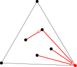
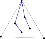
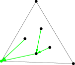
Figure 1.6: Partition of the inner edges into three spanning trees.

These orientations and colorings of the internal edges of a planar triangulation where first introduced by Schnyder [50] who proved their existence for any planar triangulation. The partition into three trees is the reason of their usual name: Schnyder woods.

Chapter 2 Generalization to 3-connected planar maps

To define Schnyder woods formally we use the following local property introduced by Schnyder [50] (see Figure 1.5):

Definition 1 (Schnyder property)

Given a map $G$, a vertex $v$ and an orientation and coloring of the edges incident to $v$ with the colors $0$, $1$, $2$, we say that $v$ satisfies the Schnyder property, if $v$ satisfies the following local property:

• Vertex $v$ has out-degree one in each color.

• The edges $e_{0}(v)$, $e_{1}(v)$, $e_{2}(v)$ leaving $v$ in colors $0$, $1$, $2$, respectively, occur in counterclockwise order.

• Each edge entering $v$ in color $i$ enters $v$ in the counterclockwise sector from $e_{i+1}(v)$ to $e_{i-1}(v)$.

Then the formal definition of Schnyder woods is the following:

Definition 2 (Schnyder wood)

Given a planar triangulation $G$, a Schnyder wood is an orientation and coloring of the inner edges of $G$ with the colors $0$, $1$, $2$ (edges are oriented in one direction only), where each inner vertex $v$ satisfies the Schnyder property.

See Figure 1.4 for an example of a Schnyder wood.

By a result of De Fraysseix and Ossona de Mendez [30], there is a bijection between orientations of the internal edges of a planar triangulation where every inner vertex has outdegree $3$ and Schnyder woods. Indeed, Chapter 1 gives the ideas behind this bijection and show how to recover the colors from the orientation.

Originally, Schnyder woods were defined only for planar triangulations [50]. Felsner [21, 22] extended this definition to planar maps. To do so he allowed edges to be oriented in one direction or in two opposite directions and when an edge is oriented in two direction, then each direction have a distinct color and is outgoing (see Figure 2.1).

Figure 2.1: The two types of edges in planar Schnyder woods

Then the formal definition of the generalization, called planar Schnyder wood in this manuscript, is the following:

Definition 3 (Planar Schnyder wood)

Given a planar map $G$. Let $x_{0}$, $x_{1}$, $x_{2}$ be three vertices occurring in counterclockwise order on the outer face of $G$. The suspension $G^{\sigma}$ is obtained by attaching a half-edge that reaches into the outer face to each of these special vertices. A planar Schnyder wood rooted at $x_{0}$, $x_{1}$, $x_{2}$ is an orientation and coloring of the edges of $G^{\sigma}$ with the colors $0$, $1$, $2$, where every edge is oriented in one direction or in two opposite directions (each direction having a distinct color and being outgoing), satisfying the following conditions:

• Every vertex satisfies the Schnyder property and the half-edge at $x_{i}$ is directed outward and colored $i$.

• There is no face whose boundary is a monochromatic cycle.

See Figure 2.2 for two examples of planar Schnyder woods.

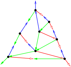
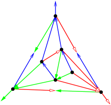
Figure 2.2: A planar Schnyder wood of a planar map and of a planar triangulation.

When there is no ambiguity we may omit the word “planar” in “planar Schnyder wood”.

Note that a planar triangulation has exactly $3n-6$ edges and this explains why in Definition 2 just inner vertices are required to satisfy the Schnyder property. There are $3$ vertices in the outer face that together should have $9$ outgoing edges in order to satisfy the Schnyder property but there is just $3$ non-colored edges on the outer face (see for instance Figure 1.4). In Definition 3 restricted to planar triangulations, the $6$ missing outgoing edges are obtained by adding $3$ half-edges reaching into the outer face and by orienting the $3$ outer edges in two directions. On the right of Figure 2.2 the triangulation of Figure 1.4 is represented with a planar Schnyder wood.

A planar map $G$ is internally 3-connected if there exists three vertices on the outer face such that the graph obtain from $G$ by adding a vertex adjacent to the three vertices is 3-connected. Miller [41] proved the following (see also [21] for existence of Schnyder woods for 3-connected planar maps and [11] where the following result is stated in this form):

Theorem 1 ([41])

A planar map admits a planar Schnyder wood if and only if it is internally 3-connected.

Consider a planar Schnyder wood. Let $G_{i}$ be the directed graph induced by the edges of color $i$ of $G$. This definition includes edges that are half-colored $i$, and in this case, the edges get only the direction corresponding to color $i$. The graph $(G_{i})^{-1}$ is the graph obtained from $G_{i}$ by reversing all its edges. The graph $G_{i}\cup G_{i-1}^{-1}\cup G_{i+1}^{-1}$ is obtained from the graph $G$ by orienting edges in one or two direction depending on whether this orientation is present in $G_{i}$, $G_{i-1}^{-1}$ or $G_{i+1}^{-1}$. Felsner [21] proved the following essential property of planar Schnyder wood:

Lemma 1 ([21])

The graph $G_{i}\cup(G_{i-1})^{-1}\cup(G_{i+1})^{-1}$ contains no directed cycle.

Every vertex, is the starting point of an outgoing edge of color $i$. Since $G_{i}$ is acyclic by Lemma 1, we have the following:

Lemma 2 ([21])

For $i\in\{0,1,2\}$, the digraph $G_{i}$ is a tree rooted at $x_{i}$.

Thus in planar Schnyder woods, we still have, like for the triangulation case, three spanning trees. But now some edges appear in two trees, so it is no more a partition of the edges into three spanning trees. Figure 2.3 illustrate this property on the planar Schnyder wood of the left of Figure 2.2.

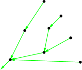
$G_{0}$	$G_{1}$	$G_{2}$

Figure 2.3: Three spanning trees.

For every vertex $v$ and color $i$, let $P_{i}(v)$ denote the directed path from $v$ to $x_{i}$, composed of edges colored $i$. Then another consequence of Lemma 1 is the following:

Lemma 3 ([21])

For every vertex $v$ and $i,j\in\{0,1,2\}$, $i\neq j$, the two paths $P_{i}(v)$ and $P_{j}(v)$ have $v$ as only common vertex.

Thus, like for triangulations, for every vertex $v$, the three monochromatic paths $P_{0}(v)$, $P_{1}(v)$, $P_{2}(v)$ do not intersect each other except on $v$. These paths divide $G$ into regions (see Figure 2.4) which form the basis of several graph drawing methods using Schnyder woods, see for instance [51, 21].

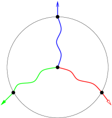
Figure 2.4: Regions delimited by the three monochromatic paths from a vertex.

Allowing edges to be oriented in one or two directions as in Definition 3 also enables to define the dual of a planar Schnyder wood. Indeed, by applying the correspondence of Figure 2.5, a planar Schnyder wood of $G^{\sigma}$ automatically defines a planar Schnyder wood of the dual map (with a special rule for the outer face that gets three vertices plus three half-edges). Figure 2.6 illustrate this property on the planar Schnyder wood of the left of Figure 2.2 where vertices of the primal are black and vertices of the dual are white (this serves as a convention for the rest of the manuscript).

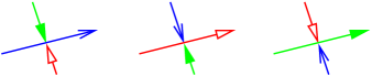
Figure 2.5: Rules for the dual Schnyder wood.

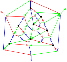
Figure 2.6: Superposition of a planar Schnyder wood and its dual.

Part II Generalization to orientable surfaces

Chapter 3 Generalization of Schnyder woods

3.1 Euler’s formula and consequences

For higher genus triangulated surfaces, a generalization of Schnyder woods has been proposed by Castelli Aleardi, Fusy and Lewiner [13], with applications to encoding. In this definition, the simplicity and the symmetry of the original definition of Schnyder woods are lost. Here we propose an alternative generalization of Schnyder woods for higher genus.

A closed curve on a surface is contractible if it can be continuously transformed into a single point. Given a graph embedded on a surface, a contractible loop is an edge forming a contractible curve. Two edges of an embedded graph are called homotopic multiple edges if they have the same extremities and their union encloses a region homeomorphic to an open disk. Except if stated otherwise, we consider graphs embedded on surfaces that do not have contractible loops nor homotopic multiple edges. Note that this is a weaker assumption, than the graph being simple, i.e. not having loops nor multiple edges. A graph embedded on a surface is called a map on this surface if all its faces are homeomorphic to open disks. A map is a triangulation if all its faces have size three. A triangle of a map is a closed walk of size $3$ enclosing a region that is homeomorphic to an open disk. This region is called the interior of the triangle. Note that a triangle is not necessarily a face of the map as its interior may be not empty. A separating triangle is a triangle whose interior is non empty. Note also that a triangle is not necessarily a cycle since non-contractible loops are allowed.

Euler’s formula says that any map on an orientable surface of genus $g$ satisfies $n-m+f=2-2g$. In particular, the plane is the surface of genus $0$, the torus the surface of genus $1$, the double torus the surface of genus $2$, etc. By Euler’s formula, a triangulation of genus $g$ has exactly $3n+6(g-1)$ edges. For a toroidal triangulation, Euler’s formula gives exactly $m=3n$ so there is hope for a nice object satisfying the Schnyder property for every vertex. But having a generalization of Schnyder woods in mind, for all $g\geq 2$ there are too many edges to force all vertices to have outdegree exactly $3$. This problem can be overcome by allowing vertices to fulfill the Schnyder property “several times”, i.e. such vertices have outdegree 3, 6, 9, etc. with the color property of Figure 1.5 repeated several times (see Figure 3.1).

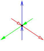
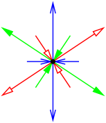
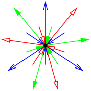
Outdegree 3	Outdegree 6	Outdegree 9

Figure 3.1: The Schnyder property repeated several times around a vertex.

In this manuscript we formalize this idea to obtain a concept of Schnyder woods applicable to general maps (not only triangulations) on arbitrary orientable surfaces.

3.2 Schnyder angle labeling

Consider a map $G$ on an orientable surface. An angle labeling of $G$ is a labeling of the angles of $G$ (i.e. face corners of $G$) in colors $0$, $1$, $2$. More formally, we denote an angle labeling by a function $\ell:\mathcal{A}\to\mathbb{Z}_{3}$, where $\mathcal{A}$ is the set of angles of $G$. Given an angle labeling, we define several properties of vertices, faces and edges that generalize the notion of Schnyder angle labeling in the planar case [24].

Consider an angle labeling $\ell$ of $G$. A vertex or a face $v$ is of type $k$, for $k\geq 1$, if the labels of the angles around $v$ form, in counterclockwise order, $3k$ nonempty intervals such that in the $j$-th interval all the angles have color $(j\mod 3)$. A vertex or a face $v$ is of type $0$, if the labels of the angles around $v$ are all of color $i$ for some $i$ in $\{0,1,2\}$.

An edge $e$ is of type $1$ or $2$ if the labels of the four angles incident to edge $e$ are, in clockwise order, $i-1$, $i$, $i$, $i+1$ for some $i$ in $\{0,1,2\}$. The edge $e$ is of type $1$ if the two angles with the same color are incident to the same extremity of $e$ and of type $2$ if the two angles are incident to the same side of $e$. An edge $e$ is of type $0$ if the labels of the four angles incident to edge $e$ are all $i$ for some $i$ in $\{0,1,2\}$ (see Figure 3.2).

If there exists a function $f:V\to\mathbb{N}$ such that every vertex $v$ of $G$ is of type $f(v)$, we say that $\ell$ is $f$-vertex. If we do not want to specify the function $f$, we simply say that $\ell$ is vertex. We sometimes use the notation $K$-vertex if the labeling is $f$-vertex for a function $f$ with $f(V)\subseteq K$. When $K=\{k\}$, i.e. $f$ is a constant function, then we use the notation $k$-vertex instead of $f$-vertex. Similarly we define face, $K$-face, $k$-face, edge, $K$-edge, $k$-edge.

The following lemma shows that property edge is the central notion here. Properties $K$-vertex and $K$-face are used to express additional requirements on the angle labellings that are considered.

Lemma 4

An edge angle labeling is vertex and face.

Proof.  Consider $\ell$ an edge angle labeling. Consider two counterclockwise consecutive angles $a,a^{\prime}$ around a vertex (or a face). Property edge implies that $\ell(a^{\prime})=\ell(a)$ or $\ell(a^{\prime})=\ell(a)+1$ (see Figure 3.2). Thus by considering all the angles around a vertex or a face, it is clear that $\ell$ is also vertex and face. $\Box$

Thus we define a Schnyder labeling as follows:

Definition 4 (Schnyder labeling)

Given a map $G$ on an orientable surface, a Schnyder labeling of $G$ is an edge angle labeling of $G$.

Figure 3.2 shows how a Schnyder labeling defines an orientation and coloring of the edges of the graph with edges oriented in one direction or in two opposite directions. Compared to Definition 3, we allow an edge to be oriented in two opposite directions that are incoming, and in this case the two direction have the same color.

Type 0	Type 1	Type 2

Figure 3.2: Correspondence between Schnyder labellings and some bi-orientations and colorings of the edges.

The correspondence of Figure 3.2 gives the following bijection, as proved by Felsner [22] (see Figure 3.3):

Proposition 1 ([22])

If $G$ is a planar map and $x_{0}$, $x_{1}$, $x_{2}$ are three vertices occurring in counterclockwise order on the outer face of $G$, then the planar Schnyder woods of $G^{\sigma}$ are in bijection with the {1,2}-edge, 1-vertex, 1-face angle labellings of $G^{\sigma}$ (with the outer face being 1-face but in clockwise order w.r.t. itself).

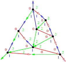
Figure 3.3: Angle labeling corresponding to a planar Schnyder wood.

In Sections 3.3 and 3.4, we show how Schnyder labellings can be used to generalize Schnyder woods on surfaces and then exhibit some properties in the dual (Section 3.5) and in the universal cover (Section 3.6). In Section 3.7, we raise some conjectures about the existence of Schnyder labeling in higher genus that leads us to consider edge, $\mathbb{N}^{*}$-vertex, $\mathbb{N}^{*}$-face angle labellings. These particular angle labellings seem to be the most interesting case of Schnyder labellings when $g\geq 1$ but the core of the structural properties (Chapters 4 and 5) is written for the general situation of edge angle labellings with no additional requirement on properties vertex and face.

3.3 Spherical Schnyder woods

We generalize angle labellings letting vertices have outdegree equal to $0\bmod 3$ and not necessarily exactly $3$ like in the previous definitions of Schnyder woods. Such a relaxation allows us to define a new kind of Schnyder wood in the plane with no “special rule” on the outer face (i.e. not just considering inner vertices like in Definition 2 and without adding half-edges reaching the outer face like in Definition 3). We call them spherical Schnyder woods since there is no face playing the particular role of the outer face.

Definition 5 (spherical Schnyder wood)

Given a planar map $G$, a spherical Schnyder wood is an orientation and coloring of the edges of $G$ with the colors $0$, $1$, $2$, where every edge is oriented in one direction or in two opposite directions (each direction having a distinct color and being outgoing), satisfying the following conditions:

• Every vertex, except exactly two vertices called poles, satisfies the Schnyder property and each pole has only incoming edges, all of the same color.

• There is no face whose boundary is a monochromatic cycle.

See Figure 3.4 for two examples of spherical Schnyder woods.

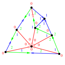
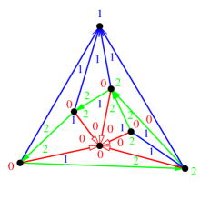
Figure 3.4: A spherical Schnyder wood of a planar map and of a planar triangulation.

Like for planar Schnyder woods, there is a bijection between spherical Schnyder woods and particular angle labellings (see Figure 3.4):

Proposition 2

If $G$ is a planar map, then the spherical Schnyder woods of $G$ are in bijection with the {1,2}-edge, {0,1}-vertex, 1-face angle labellings of $G$.

Proof.  ($\Longrightarrow$) Consider a spherical Schnyder wood of $G$. We label the angles around a pole $v$ with the color of its incident edges. We label the angles of a non-pole vertex $v$ such that all the angles in the counterclockwise sector from $e_{i+1}(v)$ to $e_{i-1}(v)$ are labeled $i$. Then one can easily check that the two poles are of type 0, that all the non-poles are of type 1 and that all the edges are of type 1 or 2. Then by Lemma 4, the labeling is also face.

It remains to prove that the labeling is 1-face. For this purpose, we count the color changes of the angles at vertices, faces and edges, and denote it by the function $c$. Since the labeling is {1,2}-edge, for an edge $e$ there are exactly three changes around $e$, so $c(e)=3$ and $\sum_{e}c(e)=3m$. These changes around an edge can happen either around one of the two incident vertices or one of the two incident faces, so $\sum_{e}c(e)=\sum_{v}c(v)+\sum_{f}c(f)$. The vertices $v$ of type 1 have $c(v)=3$. The two vertices $v$ of type 0 have $c(v)=0$. So $\sum_{v}c(v)=3(n-2)$. Thus finally, $\sum_{f}c(f)=3m-3(n-2)=3f$ (the last equality is by Euler’s formula). Since the labeling is face, we have $c(f)=0\bmod 3$ for every face $f$. As there is no face whose boundary is a monochromatic cycle, all the faces have $c(f)\geq 3$ and thus all the faces have exactly $c(f)=3$ and the labeling is 1-face.

($\Longleftarrow$) Consider a {1,2}-edge, {0,1}-vertex, 1-face angle labeling of $G$. Again, we count the color changes of the angles at vertices, faces and edges. We have $3m=\sum_{e}c(e)=\sum_{v}c(v)+\sum_{f}c(f)$ and $\sum_{f}c(f)=3f$. Then Euler’s formula gives $\sum_{v}c(v)=3m-3f=3(n-2)$. The vertices $v$ of type 1 have $c(v)=3$ and the vertices $v$ of type 0 have $c(v)=0$. So there are exactly two vertices of type 0. Consider the coloring and orientation of the edges of $G$ obtained by the correspondence shown in Figure 3.2. It is clear that every vertex, except exactly the two vertices of type 0, satisfies the Schnyder property and that each vertex of type 0 has only incoming edges, all of the same color. Since the angle labeling is 1-face, there is no face whose boundary is a monochromatic cycle as such a face is of type 0. So the considered coloring and orientation of the edges of $G$ is a spherical Schnyder wood. $\Box$

A spherical Schnyder wood of a planar triangulation has all its faces that are triangular and 1-face. Thus the three angles of a face are labels $0,1,2$ and there is no bi-directed edge. So the angle labeling is 1-edge.

Spherical Schnyder woods seem somewhat less “regular” than usual Schnyder woods. For example, the colors of the edges at the two poles can be distinct or identical and the edges having the same color can induce a connected graph or not and may contains cycles (see Figures 3.4 and 3.5).

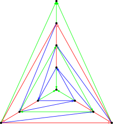
Figure 3.5: A spherical Schnyder wood of a planar triangulation where the green color has three components including the two poles.

Note that the two poles must be non-adjacent vertices since they have only incoming edges. Then it is not difficult to see that $K_{4}$ is the only planar triangulation that does not admit a spherical Schnyder wood.

Proposition 3

A planar triangulation that is not $K_{4}$ admits a spherical Schnyder wood.

Proof.  Let $G$ be a planar triangulation that is not $K_{4}$. Since $G$ is not $K_{4}$, we can consider $x_{0},x_{1},x_{2},u$ such that $x_{0}$, $x_{1}$, $x_{2}$ are the three vertices occurring in counterclockwise order on the outer face of $G$, vertex $u$ is not incident to $x_{1}$, and $x_{0}ux_{2}$ is a face of $G$. Consider a planar Schnyder wood of $G$ rooted at $x_{0}$, $x_{1}$, $x_{2}$ (see Definition 3 and example of Figure 2.2). Let $v$ be the entering vertex of $e_{1}(u)$. We now transform the planar Schnyder wood into a spherical Schnyder wood by the following:

• Remove the half-edges at $x_{0},x_{1},x_{2}$.

• Orient the three outer edges in one direction only such that $x_{0}x_{1}$ and $x_{2}x_{1}$ are entering $x_{1}$ in color $1$, and $x_{2}x_{0}$ is leaving $x_{2}$ in color $2$.

• Reverse the three edges $ux_{0},uv,ux_{2}$ such that they are entering $u$ in color $0$.

• Reverse all the edges of the path $P_{0}(v)$ from $x_{0}$ to $v$ and color them in color $2$.

• In the interior of the region delimited by $vu$, $ux_{0}$ and $P_{0}(v)$, add $+1$ to all the colors (without modifying the orientation).

Then it is not difficult to see that the obtained orientation and coloring is a spherical Schnyder wood of $G$ with poles $x_{1}$ and $u$. $\Box$

The proof of Proposition 3 gives a general method to transform a planar Schnyder wood into a spherical Schnyder wood. The spherical Schnyder wood on the right of Figure 3.4 is obtained from the one on the right of Figure 2.2 by such a transformation. This transformation can be done in a more general framework where $u,v$ are any inner vertices satisfying: $v$ is on $P_{1}(u)$ and $P_{0}(u),P_{0}(v)$ are edge disjoint. This is illustrated on Figure 3.6 where the “+1” and “-1” indicates the change of colors in the interior of the considered region.

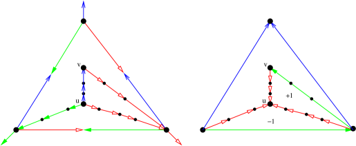
Figure 3.6: Transforming a planar Schnyder wood into a spherical Schnyder wood.

Note that it is also possible to define variants of Definition 5. For example one can allow one pole or the two poles to be in the dual map. For triangulation, this implies the use of edges of type 2 by a counting argument. Figure 3.7 gives two such examples. The example on the left of Figure 3.7 is obtained from the triangulation of Figure 2.2 by choosing an inner vertex $v$, reversing the three monochromatic paths from $v$ and removing the half edges. The example on the right of Figure 3.7 is obtained from the triangulation of Figure 2.2 by choosing an inner face $f$, reversing three paths with different colors from the three vertex of $f$, removing the half edges and orienting the edges of $f$ in both directions.

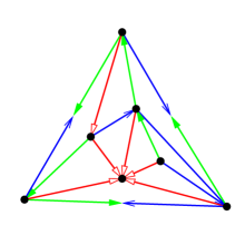
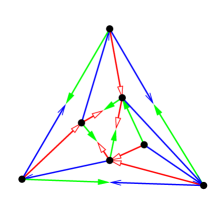
Figure 3.7: Examples of orientation

We have defined spherical Schnyder woods with poles in the primal since in the context of Schnyder woods, the objects that are considered seem to be most interesting when, for triangulation, only type 1 edges are used. Here we will not study much further these natural classes of {1,2}-edge angle labellings of planar maps.

3.4 Generalized Schnyder woods

Any map (on any orientable surface) admits a trivial edge angle labeling: the one with all angles labeled $i$ (and thus all edges, vertices and faces are of type 0). A natural non-trivial case, that is also symmetric for the duality, is to consider edge, $\mathbb{N}^{*}$-vertex, $\mathbb{N}^{*}$-face angle labellings of general maps. In planar Schnyder woods only type 1 and type 2 edges are used. Here we allow type 0 edges because they seem unavoidable for some maps (see discussion below). This suggests the following definition of Schnyder woods in higher genus.

First, the generalization of the Schnyder property is the following (see Figure 3.1):

Definition 6 (Generalized Schnyder property)

Given a map $G$ on a genus $g\geq 1$ orientable surface, a vertex $v$ and an orientation and coloring of the edges incident to $v$ with the colors $0$, $1$, $2$, we say that $v$ satisfies the generalized Schnyder property, if $v$ satisfies the following local property for $k\geq 1$:

• Vertex $v$ has out-degree $3k$.

• The edges $e_{0}(v),\ldots,e_{3k-1}(v)$ leaving $v$ in counterclockwise order are such that $e_{j}(v)$ has color $(j\bmod 3)$.

• Each edge entering $v$ in color $i$ enters $v$ in a counterclockwise sector from $e_{j}(v)$ to $e_{j+1}(v)$ (where $j$ and $j+1$ are understood modulo $3k$) with $(j\bmod 3)\neq(i\bmod 3)\neq((j+1)\bmod 3)$.

Then, the generalization of Schnyder woods is the following (where the three types of edges depicted on Figure 3.2 are allowed):

Definition 7 (Generalized Schnyder wood)

Given a map $G$ on a genus $g\geq 1$ orientable surface, a generalized Schnyder wood of $G$ is an orientation and coloring of the edges of $G$ with the colors $0$, $1$, $2$, where every edge is oriented in one direction or in two opposite directions (each direction having a distinct color and being outgoing, or each direction having the same color and being incoming), satisfying the following conditions:

• Every vertex satisfies the generalized Schnyder property (see Definition 6).

• There is no face whose boundary is a monochromatic cycle.

When there is no ambiguity we may omit the word “generalized” in “generalized Schnyder wood” or “generalized Schnyder property”.

See Figure 3.8 for two examples of Schnyder woods in the torus (where the torus is represented by a square in the plane whose opposite sides are pairwise identified).

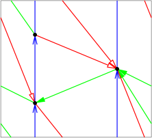
Figure 3.8: A Schnyder wood of a toroidal map and of a toroidal triangulation.

Figure 3.9 is an example of a Schnyder wood on a triangulation of the double torus. The double torus is represented by an octagon. The sides of the octagon are identified according to their labels. All the vertices of the triangulation have outdegree 3 except two vertices that have outdegree 6, which are circled. Each of the latter appears twice in the representation.

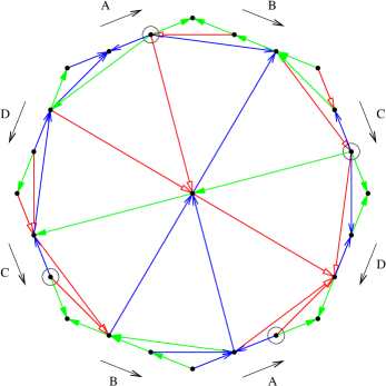
Figure 3.9: A Schnyder wood of a triangulation of the double torus.

The correspondence of Figure 3.2 immediately gives the following bijection whose proof is omitted.

Proposition 4

If $G$ is a map on a genus $g\geq 1$ orientable surface, then the generalized Schnyder woods of $G$ are in bijection with the edge, $\mathbb{N}^{*}$-vertex, $\mathbb{N}^{*}$-face angle labelings of $G$.

Note that in the examples of Figures 3.8 and 3.9, type 0 edges do not appear. However, for $g\geq 2$, there are some maps with vertex degrees and face degrees at most $5$ that admits generalized Schnyder woods. For these maps, type $0$ edges are unavoidable. Figure 3.10 gives an example of such a map for $g=2$, with a Schnyder wood that has two edges of type 0.

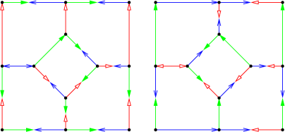
Figure 3.10: A Schnyder wood of a double-toroidal map that has two edges of type 0. Here, the two parts are toroidal and the two central faces are identified (by preserving the colors) to obtain a double-toroidal map.

3.5 Schnyder woods and duality

Given a map $G$ on an genus $g\geq 1$ orientable surface, the dual of a Schnyder wood of $G$ is the orientation and coloring of the edges of $G^{*}$ obtained by the rules represented on Figure 3.11 where the correspondence of Figure 3.2 is still valid in the dual map.

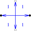
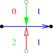
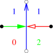
Type 0	Type 1	Type 2

Figure 3.11: Rules for the dual Schnyder wood and the corresponding angle labeling.

Note that a Schnyder wood of $G$ is an edge, $\mathbb{N}^{*}$-vertex, $\mathbb{N}^{*}$-face angle labeling of $G$ (by Proposition 4), thus an edge, $\mathbb{N}^{*}$-vertex, $\mathbb{N}^{*}$-face angle labeling of $G^{*}$ (by symmetry of the definitions vertex and face), thus a Schnyder wood of $G^{*}$. So we have the following:

Proposition 5

Given a map $G$ on a genus $g\geq 1$ orientable surface, there is a bijection between the Schnyder woods of $G$ and of its dual.

An example of a Schnyder wood of a toroidal map and its dual is given on Figure 3.12.

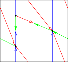
Figure 3.12: Schnyder woods of a primal and dual toroidal map.

3.6 Schnyder woods in the universal cover

We refer to [39] for the general theory of universal covers. The universal cover of the torus (resp. an orientable surface of genus $g\geq 2$) is a surjective mapping $p$ from the plane (resp. the open unit disk) to the surface that is locally a homeomorphism. If the torus is represented by a hexagon in the plane whose opposite sides are pairwise identified, then the universal cover of the torus is obtained by replicating the hexagon to tile the plane. Figure 3.13 shows how to obtain the universal cover of the double torus. The key property is that a closed curve on the surface corresponds to a closed curve in the universal cover if and only if it is contractible.

Figure 3.13: Canonical representation and universal cover of the double torus (source: Yann Ollivier http://www.yann-ollivier.org/maths/primer.php).

Universal covers can be used to represent a map on an orientable surface as an infinite planar map. Any property of the map can be lifted to its universal cover, as long as it is defined locally. Thus universal covers are an interesting tool for the study of Schnyder woods since all the definitions we have given so far are purely local.

Consider a map $G$ on a genus $g\geq 1$ orientable surface. Let $G^{\infty}$ be the infinite planar map drawn on the universal cover and defined by $p^{-1}(G)$. Note that $G$ does not have contractible loops or homotopic multiple edges if and only if $G^{\infty}$ is simple.

We need the following general lemma concerning universal covers:

Lemma 5

Suppose that for a finite set of vertices $X$ of $G^{\infty}$, the graph $G^{\infty}\setminus X$ is not connected. Then $G^{\infty}\setminus X$ has a finite connected component.

Proof.  Suppose the lemma is false and $G^{\infty}\setminus X$ is not connected and has no finite component. Then it has a face bounded by an infinite number of vertices. As the vertices of $G^{\infty}$ have bounded degree, by putting vertices $X$ back there is still a face bounded by an infinite number of vertices. The corresponding face in $G$ is not homeomorphic to an open disk, a contradiction with $G$ being a map. $\Box$

A graph is $k$-connected if it has at least $k+1$ vertices and if it stays connected after removing any $k-1$ vertices. Extending the notion of essentially 2-connectedness defined in [43] for the toroidal case, we say that $G$ is essentially $k$-connected if $G^{\infty}$ is $k$-connected. Note that the notion of being essentially $k$-connected is different from being $k$-connected. There is no implication in any direction and being essentially $k$-connected depends on the mapping (see Figure 3.14 and Figure 3.15). Note that a map is always essentially $1$-connected.

Figure 3.14: An essentially 2-connected map that is not 2-connected and an essentially 3-connected map that is not 3-connected.

Figure 3.15: Three different mappings of the same underlying 3-connected graph, which are respectively: essentially 1-connected (not essentially 2-connected), essentially 2-connected (not essentially 3-connected), essentially 3-connected (not essentially 4-connected).

Suppose now that $G$ is given with a Schnyder wood (i.e. an edge, $\mathbb{N}^{*}$-vertex, $\mathbb{N}^{*}$-face angle labeling by Proposition 4). Consider the orientation and coloring of the edges of $G^{\infty}$ corresponding to the Schnyder wood of $G$.

Let $G^{\infty}_{i}$ be the directed graph induced by the edges of color $i$ of $G^{\infty}$. This definition includes edges that are half-colored $i$, and in this case, the edges get only the direction corresponding to color $i$. The graph $(G^{\infty}_{i})^{-1}$ is the graph obtained from $G^{\infty}_{i}$ by reversing all its edges. The graph $G^{\infty}_{i}\cup(G^{\infty}_{i-1})^{-1}\cup(G^{\infty}_{i+1})^{-1}$ is obtained from the graph $G$ by orienting edges in one or two directions depending on whether this orientation is present in $G^{\infty}_{i}$, $(G^{\infty}_{i-1})^{-1}$ or $(G^{\infty}_{i+1})^{-1}$. Similarly to what happens for planar Schnyder woods (see Lemma 1), we have the following important property:

Lemma 6

The graph $G^{\infty}_{i}\cup(G^{\infty}_{i-1})^{-1}\cup(G^{\infty}_{i+1})^{-1}$ contains no directed cycle.

Proof.  Suppose there is a directed cycle in $G^{\infty}_{i}\cup(G^{\infty}_{i-1})^{-1}\cup(G^{\infty}_{i+1})^{-1}$. Let $C$ be such a cycle containing the minimum number of faces in the map $D$ with border $C$. Suppose by symmetry that $C$ turns around $D$ counterclockwisely. Every vertex of $D$ has at least one outgoing edge of color $i+1$ in $D$. So there is a cycle of color $(i+1)$ in $D$ and this cycle is $C$ by minimality of $C$. Every vertex of $D$ has at least one outgoing edge of color $i$ in $D$. So, again by minimality of $C$, the cycle $C$ is a cycle of color $i$. Thus all the edges of $C$ are oriented in color $i$ counterclockwisely and in color $i+1$ clockwisely.

By the definition of Schnyder woods, there is no face the boundary of which is a monochromatic cycle, so $D$ is not a face. Let $vx$ be an edge in the interior of $D$ that is outgoing for $v$. The vertex $v$ can be either in the interior of $D$ or in $C$ (if $v$ has more than three outgoing arcs). In both cases, $v$ has necessarily an edge $e_{i}$ of color $i$ and an edge $e_{i+1}$ of color $i+1$, leaving $v$ and in the interior of $D$. Consider $W_{i}(v)$ (resp. $W_{i+1}(v)$) a monochromatic walk starting from $e_{i}$ (resp. $e_{i+1}$), obtained by following outgoing edges of color $i$ (resp. $i+1$). By minimality of $C$ those walks are not contained in $D$. We hence have that $W_{i}(v)\setminus v$ and $W_{i+1}(v)\setminus v$ intersect $C$. Thus each of these walks contains a non-empty subpath from $v$ to $C$. The union of these two paths, plus a part of $C$ contradicts the minimality of $C$. $\Box$

Let $v$ be a vertex of $G^{\infty}$. For each color $i$, vertex $v$ is the starting vertex of some walks of color $i$, we denote the union of these walks by $P_{i}(v)$. Every vertex has at least one outgoing edge of color $i$ and the set $P_{i}(v)$ is obtained by following all these edges of color $i$ starting from $v$. The analogous of Lemma 3 is:

Lemma 7

For every vertex $v$ and $i,j\in\{0,1,2\}$, $i\neq j$, the two graphs $P_{i}(v)$ and $P_{j}(v)$ have $v$ has only common vertex.

Proof.  If $P_{i}(v)$ and $P_{j}(v)$ intersect on two vertices, then $G^{\infty}_{i}\cup(G_{j}^{{}^{\infty}})^{-1}$ contains a cycle, contradicting Lemma 6. $\Box$

Now we can prove the following:

Lemma 8

If a map $G$ on a genus $g\geq 1$ orientable surface admits a generalized Schnyder wood, then $G$ is essentially 3-connected.

Proof.  Suppose by contradiction that there exist two vertices $x,y$ of $G^{\infty}$ such that $G^{\prime}=G^{\infty}\setminus\{x,y\}$ is not connected. Then, by Lemma 5, the graph $G^{\prime}$ has a finite connected component $R$. Let $v$ be a vertex of $R$. By Lemma 6, for $0\leq i\leq 2$, the graph $P_{i}(v)$ does not lie in $R$ so it intersects either $x$ or $y$. So for two distinct colors $i,j$, the two graphs $P_{i}(v)$ and $P_{j}(v)$ intersect in a vertex distinct from $v$, a contradiction to Lemma 7. $\Box$

3.7 Conjectures on the existence of Schnyder woods

Proving that every triangulation on a genus $g\geq 1$ orientable surface admits a 1-edge angle labeling would imply the following theorem of Barát and Thomassen [3]:

Theorem 2 ([3])

A simple triangulation on a genus $g\geq 1$ orientable surface admits an orientation of its edges such that every vertex has outdegree divisible by $3$.

Recently, Theorem 2 has been improved by Albar, Gonçalves and Knauer [1]:

Theorem 3 ([1])

A simple triangulation on a genus $g\geq 1$ orientable surface admits an orientation of its edges such that every vertex has outdegree at least $3$, and divisible by $3$.

Note that Theorems 2 and 3 are proved only in the case of simple triangulations (i.e. no loops and no multiple edges). We believe them to be true also for non-simple triangulations without contractible loops nor homotopic multiple edges.

Theorem 3 suggests the existence of 1-edge angle labelings with no sinks, i.e. 1-edge, $\mathbb{N}^{*}$-vertex angle labelings. One can easily check that in a triangulation, a 1-edge angle labeling is also 1-face. Thus one can hope that a triangulation on a genus $g\geq 1$ orientable surface admits a 1-edge, $\mathbb{N}^{*}$-vertex, 1-face angle labeling. Note that a 1-edge, 1-face angle labeling of a map implies that faces have size three. So we propose the following conjecture, whose “only if” part follows from the previous sentence:

Conjecture 1

A map on a genus $g\geq 1$ orientable surface admits a 1-edge, $\mathbb{N}^{*}$-vertex, 1-face angle labeling if and only if it is a triangulation.

If true, Conjecture 1 would strengthen Theorem 3 in two ways. First, it considers more triangulations (not only simple ones). Second, it requires the coloring property of Figure 3.1 around vertices.

How about general maps? We propose the following conjecture, whose “only if” part is implied by Proposition 4 and Lemma 8:

Conjecture 2

A map on a genus $g\geq 1$ orientable surface admits an edge, $\mathbb{N}^{*}$-vertex, $\mathbb{N}^{*}$-face angle labeling if and only if it is essentially 3-connected.

Note that the graph of Figure 3.10 is essentially 3-connected and has no $\{1,2\}$-edge angle labeling. So Conjecture 2 is false without edges of type 0. This explains why we have introduced edges of type 0 that do not appear in the planar case.

Conjecture 2 implies Conjecture 1 since for a triangulation every face would be of type 1, and thus every edge would be of type 1. The case $g=1$ of Conjecture 2 is proved in this manuscript (see Part III) whereas both conjectures are open for $g\geq 2$.

Chapter 4 Characterization of Schnyder orientations

4.1 A bit of homology

In the next sections, we need a bit of surface homology of general maps, which we discuss now. For a deeper introduction to homology we refer to [32].

For the sake of generality, in this subsection we consider that maps may have loops or multiple edges. Consider a map $G=(V,E)$ on an orientable surface of genus $g$, given with an arbitrary orientation of its edges. This fixed arbitrary orientation is implicit in all the paper and is used to handle flows. A flow $\phi$ on $G$ is a vector in $\mathbb{Z}^{|E|}$. For any $e\in E$, we denote by $\phi_{e}$ the coordinate $e$ of $\phi$.

A walk $W$ of $G$ is a sequence of edges with a direction of traversal such that the ending point of an edge is the starting point of the next edge. A walk is closed if the start and end vertices coincide. A walk has a characteristic flow $\phi(W)$ defined by:

$$\phi(W)_{e}:=\#\text{times }W\text{ traverses }e\text{ forward}-\#\text{times }\\ W\text{ traverses }e\text{ backward}$$

This definition naturally extends to sets of walks. From now on we consider that a set of walks and its characteristic flow are the same object and by abuse of notation we can write $W$ instead of $\phi(W)$. We do the same for oriented subgraphs, i.e. subgraphs that can be seen as a set of walks.

A facial walk is a closed walk bounding a face. Let $\mathcal{F}$ be the set of counterclockwise facial walks and let $\mathbb{F}={<}\phi(\mathcal{F}){>}$ the subgroup of $\mathbb{Z}^{E}$ generated by $\mathcal{F}$. Two flows $\phi,\phi^{\prime}$ are homologous if $\phi-\phi^{\prime}\in\mathbb{F}$. They are reversely homologous if $\phi+\phi^{\prime}\in\mathbb{F}$. They are weakly homologous if they are homologous or reversely homologous. We say that a flow $\phi$ is $0$-homologous if it is homologous to the zero flow, i.e. $\phi\in\mathbb{F}$.

Let $\mathcal{W}$ be the set of closed walks and let $\mathbb{W}={<}\phi(\mathcal{W}){>}$ the subgroup of $\mathbb{Z}^{E}$ generated by $\mathcal{W}$. The group $H(G)=\mathbb{W}/\mathbb{F}$ is the first homology group of $G$. It is well-known that $H(G)\cong\mathbb{Z}^{2g}$ only depends on the genus of the map.

A set $\{B_{1},\ldots,B_{2g}\}$ of (closed) walks of $G$ is said to be a homology-basis if the equivalence classes of their characteristic vectors $\{[\phi(B_{1})],\ldots,[\phi(B_{2g})]\}$ generate $H(G)$. Then for any closed walk $W$ of $G$, we have $W=\sum_{F\in\mathcal{F}}\lambda_{F}F+\sum_{1\leq i\leq 2g}\mu_{i}B_{i}$ for some $\lambda\in\mathbb{Z}^{f},\mu\in\mathbb{Z}^{2g}$. Moreover one of the $\lambda_{F}$ can be set to zero (and then all the other coefficients are unique).

For any map, there exists a set of cycles that forms a homology-basis and it is computationally easy to build. A possible way to do this is by considering a spanning tree $T$ of $G$, and a spanning tree $T^{*}$ of $G^{*}$ that contains no edges dual to $T$. By Euler’s formula, there are exactly $2g$ edges in $G$ that are not in $T$ nor dual to edges of $T^{*}$. Each of these $2g$ edges forms a unique cycle with $T$. It is not hard to see that this set of cycles, given with any direction of traversals, forms a homology-basis. Moreover, note that the intersection of any pair of these cycles is either a single vertex or a common path.

The edges of the dual map $G^{*}$ of $G$ are oriented such that the dual edge $e^{*}$ of an edge $e$ of $G$ goes from the face on the right of $e$ to the face on the left of $e$. Let $\mathcal{F}^{*}$ be the set of counterclockwise facial walks of $G^{*}$. Consider $\{B^{*}_{1},\ldots,B^{*}_{2g}\}$ a set of cycles of $G^{*}$ that form a homology-basis. Let $p$ be a flow of $G$ and $d$ a flow of $G^{*}$. We define the following:

$$\beta(p,d)=\sum_{e\in G}p_{e}d_{e^{*}}$$

Note that $\beta$ is a bilinear function.

Lemma 9

Given two flows $\phi,\phi^{\prime}$ of $G$, the following properties are equivalent to each other:

1. The two flows $\phi,\phi^{\prime}$ are homologous.

2. For any closed walk $W$ of $G^{*}$ we have $\beta(\phi,W)=\beta(\phi^{\prime},W)$.

3. For any $F\in\mathcal{F^{*}}$, we have $\beta(\phi,F)=\beta(\phi^{\prime},F)$, and, for any $1\leq i\leq 2g$, we have $\beta(\phi,B^{*}_{i})=\beta(\phi^{\prime},B^{*}_{i})$.

Proof.  $(1.\Longrightarrow 3.)$ Suppose that $\phi,\phi^{\prime}$ are homologous. Then we have $\phi-\phi^{\prime}=\sum_{F\in\mathcal{F}}\lambda_{F}F$ for some $\lambda\in\mathbb{Z}^{f}$. It is easy to see that, for any closed walk $W$ of $G^{*}$, a facial walk $F\in\mathcal{F}$ satisfies $\beta(F,W)=0$, so $\beta(\phi,W)=\beta(\phi^{\prime},W)$ by linearity of $\beta$.

$(3.\Longrightarrow 2.)$ Suppose that for any $F\in\mathcal{F^{*}}$, we have $\beta(\phi,F)=\beta(\phi^{\prime},F)$, and, for any $1\leq i\leq 2g$, we have $\beta(\phi,B^{*}_{i})=\beta(\phi^{\prime},B^{*}_{i})$. Let $W$ be any closed walk of $G^{*}$. We have $W=\sum_{F\in\mathcal{F}^{*}}\lambda_{F}F+\sum_{1\leq i\leq 2g}\mu_{i}B^{*}_{i}$ for some $\lambda\in\mathbb{Z}^{f},\mu\in\mathbb{Z}^{2g}$. Then by linearity of $\beta$ we have $\beta(\phi,W)=\beta(\phi^{\prime},W)$.

$(2.\Longrightarrow 1.)$ Suppose $\beta(\phi,W)=\beta(\phi^{\prime},W)$ for any closed walk $W$ of $G^{*}$. Let $z=\phi-\phi^{\prime}$. Thus $\beta(z,W)=0$ for any closed walk $W$ of $G^{*}$. We label the faces of $G$ with elements of $\mathbb{Z}$ as follows. Choose an arbitrary face $F_{0}$ and label it $0$. Then, consider any face $F$ of $G$ and a path $P_{F}$ of $G^{*}$ from $F_{0}$ to $F$. Label $F$ with $\ell_{F}=\beta(z,P_{F})$. Note that the label of $F$ is independent from the choice of $P_{F}$. Indeed, for any two paths $P_{1},P_{2}$ from $F_{0}$ to $F$, we have $P_{1}-P_{2}$ is a closed walk, so $\beta(z,P_{1}-P_{2})=0$ and thus $\beta(z,P_{1})=\beta(z,P_{2})$. Let us show that $z=\sum_{F\in\mathcal{F}}\ell_{F}\phi(F)$.

$$\sum_{F\in\mathcal{F}}\ell_{F}\phi(F) =\sum_{e\in G}\left(\ell_{F_{2}}-\ell_{F_{1}}\right)\phi(e) F_{2} e F_{1}$$ (face is on the left of and on the right)

$$=\sum_{e\in G}\left(\beta(z,P_{F_{2}})-\beta(z,P_{F_{1}})\right)\phi(e) \ell_{F}$$ (definition of )

$$=\sum_{e\in G}\beta(z,P_{F_{2}}-P_{F_{1}})\phi(e) \beta$$ (linearity of )

$$=\sum_{e\in G}\beta(z,e^{*})\phi(e) P_{F_{1}}+e^{*}-P_{F_{2}}$$ ( is a closed walk)

$$=\sum_{e\in G}\left(\sum_{e^{\prime}\in G}z_{e^{\prime}}\phi(e^{*})_{e^{\prime*}}\right)\phi(e) \beta$$ (definition of )

$$=\sum_{e\in G}z_{e}\phi(e)$$

$$=z$$

So $z\in\mathbb{F}$ and thus $\phi,\phi^{\prime}$ are homologous. $\Box$

4.2 General characterization

By a result of De Fraysseix and Ossona de Mendez [30], there is a bijection between orientations of the internal edges of a planar triangulation where every inner vertex has outdegree $3$ and Schnyder woods. Thus, any orientation with the proper outdegree corresponds to a Schnyder wood. This is not true in higher genus as already in the torus, there exist orientations that do not correspond to any Schnyder wood (see Figure 4.1). In this section, we characterize orientations that correspond to Schnyder angle labelings.

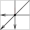
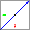
Figure 4.1: Two different orientations of a toroidal triangulation. Only the one on the right corresponds to a Schnyder wood.

Consider a map $G$ on an orientable surface of genus $g$. The mapping of Figure 3.2 shows how a Schnyder labeling of $G$ can be mapped to an orientation of the edges with edges oriented in one direction or in two opposite directions. These edges can be defined more naturally in the primal-dual-completion of $G$.

The primal-dual-completion $\hat{G}$ is the map obtained from simultaneously embedding $G$ and $G^{*}$ such that vertices of $G^{*}$ are embedded inside faces of $G$ and vice-versa. Moreover, each edge crosses its dual edge in exactly one point in its interior, which also becomes a vertex of $\hat{G}$. Hence, $\hat{G}$ is a bipartite graph with one part consisting of primal-vertices and dual-vertices and the other part consisting of edge-vertices (of degree $4$). Each face of $\hat{G}$ is a quadrangle incident to one primal-vertex, one dual-vertex and two edge-vertices. Actually, the faces of $\hat{G}$ are in correspondence with the angles of $G$. This means that angle labelings of $G$ correspond to face labelings of $\hat{G}$.

Given $\alpha:V\to\mathbb{N}$, an orientation of $G$ is an $\alpha$-orientation [23] if for every vertex $v\in V$ its outdegree $d^{+}(v)$ equals $\alpha(v)$. We call an orientation of $\hat{G}$ a $\bmod_{3}$-orientation if it is an $\alpha$-orientation for a function $\alpha$ satisfying :

$$\alpha(v)=\begin{cases}0\bmod 3&\text{if }v\text{ is a primal- or dual-vertex},\\ 1\bmod 3&\text{if }v\text{ is an edge-vertex.}\\ \end{cases}$$

Note that an Schnyder labeling of $G$ corresponds to a $\bmod_{3}$-orientation of $\hat{G}$, by the mapping of Figure 4.2, where the three types of edges are represented. Indeed, type 0 corresponds to an edge-vertex of outdegree $4$. Type 1 and type 2 both correspond to an edge-vertex of outdegree $1$; in type 1 (resp. type 2) the outgoing edge goes to a primal-vertex (resp. dual-vertex). In all cases we have $d^{+}(v)=1\bmod 3$ if $v$ is an edge-vertex. By Lemma 4, the labeling is also vertex and face. Thus $d^{+}(v)=0\bmod 3$ if $v$ is a primal- or dual-vertex.

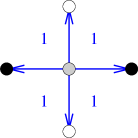
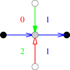
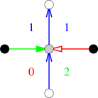
Type 0	Type 1	Type 2

Figure 4.2: How to map a Schnyder labeling to a $\bmod_{3}$-orientation of the primal-dual completion. Primal-vertices are black, dual-vertices are white and edge-vertices are gray. This serves as a convention for the other figures.

Figure 4.3 represent the primal-dual completion of the toroidal map of Figure 3.12 with a Schnyder labeling and the corresponding orientation and coloring of its edges. Note that it corresponds to a superposition of the primal and dual Schnyder woods of Figure 3.12.

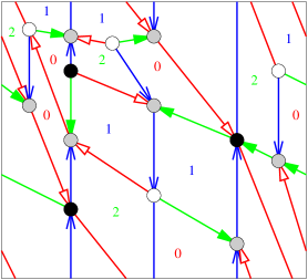
Figure 4.3: Primal-dual completion of a toroidal map given with a Schnyder labeling and the corresponding orientation and coloring.

As mentioned earlier, De Fraysseix and Ossona de Mendez [30] give a bijection between internal 3-orientations and Schnyder woods of planar triangulations. Felsner [23] generalizes this result for planar Schnyder woods and orientations of the primal-dual completion having prescribed out-degrees: $3$ for primal- or dual-vertices and $1$ for edges-vertices. The situation is more complicated in higher genus (see Figure 4.1). It is not enough to prescribe outdegrees in order to characterize orientations corresponding to Schnyder labelings.

We call an orientation of $\hat{G}$ corresponding to a Schnyder labeling of $G$ a Schnyder orientation. Note that with our definition of generalized Schnyder wood, a Schnyder orientation corresponds to a Schnyder wood if and only if $d^{+}(v)>0$ for any primal- or dual-vertex $v$ (i.e. vertex or face of type 0 are allowed in Schnyder labelings/orientations but not in Schnyder woods). In this section we characterize which orientations of $\hat{G}$ are Schnyder orientations.

Consider an orientation of the primal-dual completion $\hat{G}$. Let ${Out}=\{(u,v)\in E(\hat{G})\mid v\text{ is an edge-vertex}\}$, i.e. the set of edges of $\hat{G}$ which are going from a primal- or dual-vertex to an edge-vertex. We call these edges out-edges. For $\phi$ a flow of the dual of the primal-dual completion $\hat{G}^{*}$, we define $\delta(\phi)=\beta({Out},\phi)$. More intuitively, if $W$ is a walk of $\hat{G}^{*}$, then:

$$\begin{array}[]{ll}\delta(W)=&\ \ \#\text{out-edges crossing }W\text{ from left to right}\\ &-\#\text{out-edges crossing }W\text{ from right to left}.\end{array}$$

The bilinearity of $\beta$ implies the linearity of $\delta$.

The following lemma gives a necessary and sufficient condition for an orientation to be a Schnyder orientation.

Lemma 10

An orientation of $\hat{G}$ is a Schnyder orientation if and only if any closed walk $W$ of $\hat{G}^{*}$ satisfies $\delta(W)=0\bmod 3$.

Proof.  $(\Longrightarrow)$ Consider an edge angle labeling $\ell$ of $G$ and the corresponding Schnyder orientation (see Figure 4.2). Figure 4.4 illustrates how $\delta$ counts the variation of the label when going from one face of $\hat{G}$ to another face of $\hat{G}$ . The represented cases correspond to a walk $W$ of $\hat{G}^{*}$ consisting of just one edge. If the edge of $\hat{G}$ crossed by $W$ is not an out-edge, then the two labels in the face are the same and $\delta(W)=0$. If the edge crossed by $W$ is an out-edge, then the labels differ by one. If $W$ is going counterclockwise around a primal- or dual-vertex, then the label increases by $1\bmod 3$ and $\delta(W)=1$. If $W$ is going clockwise around a primal- or dual-vertex then the label decreases by $1\bmod 3$ and $\delta(W)=-1$. One can check that this is consistent with all the edges depicted in Figure 4.2. Thus for any walk $W$ of $\hat{G}^{*}$ from a face $F$ to a face $F^{\prime}$, the value of $\delta(W)\bmod 3$ is equal to $\ell(F^{\prime})-\ell(F)\bmod 3$. Thus if $W$ is a closed walk then $\delta(W)=0\bmod 3$.

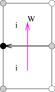
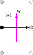
$\delta(W)=0$	$\delta(W)=1$

Figure 4.4: How $\delta$ counts the variation of the labels.

$(\Longleftarrow)$ Consider an orientation of $\hat{G}$ such that any closed walk $W$ of $\hat{G}^{*}$ satisfies $\delta(W)=0\bmod 3$. Pick any face $F_{0}$ of $\hat{G}$ and label it $0$. Consider any face $F$ of $\hat{G}$ and a path $P$ of $\hat{G}^{*}$ from $F_{0}$ to $F$. Label $F$ with the value $\delta(P)\bmod 3$. Note that the label of $F$ is independent from the choice of $P$ as for any two paths $P_{1},P_{2}$ going from $F_{0}$ to $F$, we have $\delta(P_{1})=\delta(P_{2})\bmod 3$ since $\delta(P_{1}-P_{2})=0\bmod 3$ as $P_{1}-P_{2}$ is a closed walk.

Consider an edge-vertex $v$ of $\hat{G}$ and a walk $W$ of $\hat{G}^{*}$ going clockwise around $v$. By assumption $\delta(W)=0\bmod 3$ and $d(v)=4$ so $d^{+}(v)=1\bmod 3$. One can check (see Figure 4.2) that around an edge-vertex $v$ of outdegree $4$, all the labels are the same and thus $v$ corresponds to an edge of $G$ of type 0. One can also check that around an edge-vertex $v$ of outdegree $1$, the labels are in clockwise order, $i-1$, $i$, $i$, $i+1$ for some $i$ in $\{0,1,2\}$ where the two faces with the same label are incident to the outgoing edge of $v$. Thus $v$ corresponds to an edge of $G$ of type 1 or 2 depending on the fact that the outgoing edge reaches a primal- or a dual-vertex. So the obtained labeling of the faces of $\hat{G}$ corresponds to an edge angle labeling of $G$ and the considered orientation is a Schnyder orientation. $\Box$

We now study properties of $\delta$ w.r.t. homology in order to simplify the condition of Lemma 10 that concerns any closed walk of $\hat{G}^{*}$.

Let $\hat{\mathcal{F}^{*}}$ be the set of counterclockwise facial walks of $\hat{G}^{*}$.

Lemma 11

In a $\bmod_{3}$-orientation of $\hat{G}$, any $F\in\hat{\mathcal{F}^{*}}$ satisfies $\delta(F)=0\bmod 3$.

Proof.  If $F$ corresponds to an edge-vertex $v$ of $\hat{G}$, then $v$ has degree exactly $4$ and outdegree $1$ or $4$ by definition of $\bmod_{3}$-orientations. So there are exactly $0$ or $3$ out-edges crossing $F$ from right to left, and $\delta(F)=0\bmod 3$.

If $F$ corresponds to a primal- or dual-vertex $v$, then $v$ has outdegree $0\bmod 3$ by definition of $\bmod_{3}$-orientations. So there are exactly $0\bmod 3$ out-edges crossing $F$ from left to right, and $\delta(F)=0\bmod 3$. $\Box$

Lemma 12

In a $\bmod_{3}$-orientation of $\hat{G}$, if $\{B_{1},\ldots,B_{2g}\}$ is a set of cycles of $\hat{G}^{*}$ that forms a homology-basis, then for any closed walk $W$ of $\hat{G}^{*}$ homologous to $\mu_{1}B_{1}+\cdots+\mu_{2g}B_{2g}$, $\mu\in\mathbb{Z}^{2g}$ we have $\delta(W)=\mu_{1}\delta(B_{1})+\cdots+\mu_{2g}\delta(B_{2g})\bmod 3$.

Proof.  We have $W=\sum_{F\in\hat{\mathcal{F}^{*}}}\lambda_{F}F+\sum_{1\leq i\leq 2g}\mu_{i}B_{i}$ for some $\lambda\in\mathbb{Z}^{f}$, $\mu\in\mathbb{Z}^{2g}$. Then by linearity of $\delta$ and Lemma 11, the lemma follows. $\Box$

Lemma 12 can be used to simplify the condition of Lemma 10 and show that if $\{B_{1},\ldots,B_{2g}\}$ is a set of cycles of $\hat{G}^{*}$ that forms a homology-basis, then an orientation of $\hat{G}$ is a Schnyder orientation if and only if it is a $\bmod_{3}$-orientation such that $\delta(B_{i})=0\bmod 3$, for all $1\leq i\leq 2g$. Now we define a simpler function $\gamma$ that is used to formulate a similar characterization result but with $\gamma$ (see Theorem 4).

Consider a (not necessarily directed) cycle $C$ of $G$ or $G^{*}$ together with a direction of traversal. We associate to $C$ its corresponding cycle in $\hat{G}$ denoted by $\hat{C}$. We define $\gamma(C)$ by:

$$\gamma(C)=\#\ \text{edges of $\hat{G}$ leaving $\hat{C}$ on its right}-\#\ \text{edges of $\hat{G}$ leaving $\hat{C}$ on its left}$$

Since it considers cycles of $\hat{G}$ instead of walks of $\hat{G}^{*}$, it is easier to deal with parameter $\gamma$ rather than parameter $\delta$. However $\gamma$ does not enjoy the same property w.r.t. homology as $\delta$. For homology we have to consider walks as flows, but two walks going several time through a given vertex may have the same characteristic flow but different $\gamma$. This explains why $\delta$ is defined first. Now we adapt the results for $\gamma$.

The value of $\gamma$ is related to $\delta$ by the next lemmas. Let $C$ be a cycle of $G$ or $G^{*}$ with a direction of traversal. Let $W_{L}(C)$ be the closed walk of $\hat{G}^{*}$ just on the left of $C$ and going in the same direction as $C$ (i.e. $W_{L}(C)$ is composed of the dual edges of the edges of $\hat{G}$ incident to the left of $\hat{C}$). Note that since the faces of $\hat{G}^{*}$ have exactly one incident vertex that is a primal-vertex, walk $W_{L}(C)$ is in fact a cycle of $\hat{G}^{*}$. Similarly, let $W_{R}(C)$ be the cycle of $\hat{G}^{*}$ just on the right of $C$.

Lemma 13

Consider an orientation of $\hat{G}$ and a cycle $C$ of $G$, then $\gamma(C)=\delta(W_{L}(C))+\delta(W_{R}(C))$.

Proof.  We consider the different cases that can occur. An edge that is entering a primal-vertex of $\hat{C}$, is not counting in either $\gamma(C),\delta(W_{L}(C)),\delta(W_{R}(C))$. An edge that is leaving a primal-vertex of $\hat{C}$ from its right side (resp. left side) is counting $+1$ (resp. $-1$) for $\gamma(C)$ and $\delta(W_{R}(C))$ (resp. $\delta(W_{L}(C))$).

For edges incident to edge-vertices of $\hat{C}$ both sides have to be considered at the same time. Let $v$ be an edge-vertex of $\hat{C}$. Vertex $v$ is of degree $4$ so it has exactly two edges incident to $\hat{C}$ and not on $C$. One of these edge, $e_{L}$, is on the left side of $\hat{C}$ and dual to an edge of $W_{L}(C)$. The other edge, $e_{R}$, is on the right side of $\hat{C}$ and dual to an edge of $W_{R}(C)$. If $e_{L}$ and $e_{R}$ are both incoming edges for $v$, then $e_{R}$ (resp. $e_{L}$) is counting $-1$ (resp. $+1$) for $\delta(W_{R}(C))$ (resp. $\delta(W_{L}(C))$) and not counting for $\gamma(C)$. If $e_{L}$ and $e_{R}$ are both outgoing edges for $v$, then $e_{R}$ and $e_{L}$ are not counting for both $\delta(W_{R}(C))$, $\delta(W_{L}(C))$ and sums to zero for $\gamma(C)$. If $e_{L}$ is incoming and $e_{R}$ is outgoing for $v$, then $e_{R}$ (resp. $e_{L}$) is counting $0$ (resp. $+1$) for $\delta(W_{R}(C))$ (resp. $\delta(W_{L}(C))$), and counting $+1$ (resp. $0$) for $\gamma(C)$. The last case, $e_{L}$ is outgoing and $e_{R}$ is incoming, is symmetric and one can see that in the four cases we have that $e_{L}$ and $e_{R}$ count the same for $\gamma(C)$ and $\delta(W_{L}(C))+\delta(W_{R}(C))$. Thus finally $\gamma(C)=\delta(W_{L}(C))+\delta(W_{R}(C))$. $\Box$

Lemma 14

In a $\bmod_{3}$-orientation of $G$, a cycle $C$ of $G$ satisfies

$$\delta(W_{L}(C))=0\bmod 3\ \ \text{and}\ \ \delta(W_{R}(C))=0\bmod 3\iff\gamma(C)=0\bmod 3$$

Proof.  ($\Longrightarrow$) Clear by Lemma 13.

($\Longleftarrow$) Suppose that $\gamma(C)=0\bmod 3$. Let $x_{L}$ (resp. $y_{L}$) be the number of edges of $\hat{G}$ that are dual to edges of $W_{L}(C)$, that are outgoing for a primal-vertex of $\hat{C}$ (resp. incoming for an edge-vertex of $\hat{C}$). Similarly, let $x_{R}$ (resp. $y_{R}$) be the number of edges of $\hat{G}$ that are dual to edges of $W_{R}(C)$, that are outgoing for a primal-vertex of $\hat{C}$ (resp. incoming for an edge-vertex of $\hat{C}$). So $\delta(W_{L}(C))=y_{L}-x_{L}$ and $\delta(W_{R}(C))=x_{R}-y_{R}$. So by Lemma 13, $\gamma(C)=\delta(W_{L}(C))+\delta(W_{R}(C))=(y_{L}+x_{R})-(x_{L}+y_{R})=0\bmod 3$.

Let $k$ be the number of vertices of $C$. So $\hat{C}$ has $k$ primal-vertices, $k$ edge-vertices and $2k$ edges. Edge-vertices have degree $4$, one incident edge on each side of $\hat{C}$ and outdegree $1\bmod 3$. So their total number of outgoing edges not in $\hat{C}$ is $2k-(y_{L}+y_{R})$ and their total number of outgoing edges in $\hat{C}$ is $k-2k+(y_{L}+y_{R})\bmod 3$. Primal-vertices have outdegree $(0\bmod 3)$ so their total number of outgoing edges on $\hat{C}$ is $-(x_{L}+x_{R})\bmod 3$. So in total $2k=(y_{L}+y_{R})-k-(x_{L}+x_{R})\bmod 3$. So $(y_{L}+y_{R})-(x_{L}+x_{R})=0\bmod 3$. By combining this with plus (resp. minus) $(y_{L}+x_{R})-(x_{L}+y_{R})=0\bmod 3$, one obtains that $2\delta(W_{L}(C))=2(y_{L}-x_{L})=0\bmod 3$ (resp. $2\delta(W_{R}(C))=2(x_{R}-y_{R})=0\bmod 3$). Since $\delta(W_{L}(C))$ and $\delta(W_{R}(C))$ are integer one obtains $\delta(W_{L}(C))=0\bmod 3$ and $\delta(W_{R}(C))=0\bmod 3$. $\Box$

Finally we have the following characterization theorem concerning Schnyder orientations:

Theorem 4

Consider a map $G$ on an orientable surface of genus $g$. Let $\{B_{1},\ldots,B_{2g}\}$ be a set of cycles of $G$ that forms a homology-basis. An orientation of $\hat{G}$ is a Schnyder orientation if and only if it is a $\bmod_{3}$-orientation such that $\gamma(B_{i})=0\bmod 3$, for all $1\leq i\leq 2g$.

Proof.  $(\Longrightarrow)$ Consider an edge angle labeling $\ell$ of $G$ and the corresponding Schnyder orientation (see Figure 4.2). Type 0 edges correspond to edge-vertices of outdegree $4$, while type 1 and 2 edges correspond to edge-vertices of outdegree $1$. Thus $d^{+}(v)=1\bmod 3$ if $v$ is an edge-vertex. By Lemma 4, the labeling is vertex and face. Thus $d^{+}(v)=0\bmod 3$ if $v$ is a primal- or dual-vertex. So the orientation is a $\bmod_{3}$-orientation. By Lemma 10, we have $\delta(W)=0\bmod 3$ for any closed walk $W$ of $\hat{G}^{*}$. So we have $\delta(W_{L}(B_{1})),\ldots,\delta(W_{L}(B_{2g}))$, $\delta(W_{R}(B_{1})),\ldots,\delta(W_{R}(B_{2g}))$ are all equal to $0\bmod 3$. Thus, by Lemma 14, we have $\gamma(B_{i})=0\bmod 3$, for all $1\leq i\leq 2g$.

$(\Longleftarrow)$ Consider a $\bmod_{3}$-orientation of $G$ such that $\gamma(B_{i})=0\bmod 3$, for all $1\leq i\leq 2g$. By Lemma 14, we have $\delta(W_{L}(B_{i}))=0\bmod 3$ for all $1\leq i\leq 2g$. Moreover $\{W_{L}(B_{1}),\ldots,W_{L}(B_{2g})\})$ forms a homology-basis. So by Lemma 12, $\delta(W)=0\bmod 3$ for any closed walk $W$ of $\hat{G}^{*}$. So the orientation is a Schnyder orientation by Lemma 10. $\Box$

The condition of Theorem 4 is easy to check: choose $2g$ cycles that form a homology-basis and check whether $\gamma$ equals $0\bmod 3$ for each of them.

When restricted to triangulations and to edges of type $1$ only, the definition of $\gamma$ can be simplified. Consider a triangulation $G$ on an orientable surface of genus $g$ and an orientation of the edges of $G$. Figure 4.5 shows how to transform the orientation of $G$ into an orientation of $\hat{G}$. Note that all the edge-vertices have outdegree exactly $1$. Furthermore, all the dual-vertices only have outgoing edges and since we are considering triangulations they have outdegree exactly $3$.

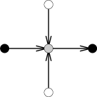
$G$	$\hat{G}$

Figure 4.5: How to transform an orientation of a triangulation $G$ into an orientation of $\hat{G}$.

Then the definition of $\gamma$ can be simplified by the following:

$$\gamma(C)=\#\ \text{edges of ${G}$ leaving ${C}$ on its right}-\#\ \text{edges of ${G}$ leaving ${C}$ on its left}$$

Note that comparing to the general definition of $\gamma$, just the symbol  $\hat{}$  on $\hat{C}$ have been removed.

The orientation of the toroidal triangulation on the left of Figure 4.1 is an example of a 3-orientation of a toroidal triangulation where some non-contractible cycles have value $\gamma$ not equal to $0\bmod 3$. The value of $\gamma$ for the three loops is $2,0$ and $-2$. This explains why this orientation does not correspond to a Schnyder wood. On the contrary, on the right of the figure, the three loops have $\gamma$ equal to $0$ and we have a Schnyder wood.

Chapter 5 Structure of Schnyder orientations

5.1 Transformations between Schnyder orientations

We investigate the structure of the set of Schnyder orientations of a given graph. For that purpose we need some definitions that are given on a general map $G$ and then applied to $\hat{G}$.

Consider a map $G$ on an orientable surface of genus $g$. Given two orientations $D$ and $D^{\prime}$ of $G$, let $D\setminus D^{\prime}$ denote the subgraph of $D$ induced by the edges that are not oriented as in $D^{\prime}$.

An oriented subgraph $T$ of $G$ is partitionable if its edge set can be partitioned into three sets $T_{0}$, $T_{1}$, $T_{2}$ such that all the $T_{i}$ are pairwise homologous, i.e. $T_{i}-T_{j}\in\mathbb{F}$ for $i,j\in\{0,1,2\}$. An oriented subgraph $T$ of $G$ is called a topological Tutte-orientation if $\beta(T,W)=0\bmod 3$ for every closed walk $W$ in $G^{*}$ (more intuitively, the number of edges crossing $W$ from left to right minus the number of those crossing $W$ from right to left is divisible by three).

The name “topological Tutte-orientation” comes from the fact that an oriented graph $T$ is called a Tutte-orientation if the difference of outdegree and indegree is divisible by three, i.e. $d^{+}(v)-d^{-}(v)=0\bmod 3$, for every vertex $v$. So a topological Tutte-orientation is a Tutte orientation, since the latter requires the condition of the topological Tutte orientation only for the walks $W$ of $G^{*}$ going around a vertex $v$ of $G$.

The notions of partitionable and topological Tutte-orientation are equivalent:

Lemma 15

An oriented subgraph of $G$ is partitionable if and only if it is a topological Tutte-orientation.

Proof.  $(\Longrightarrow)$ If $T$ is partitionable, then by definition it is the disjoint union of three homologous edge sets $T_{0}$, $T_{1}$, and $T_{2}$. Hence by Lemma 9, $\beta(T_{0},W)=\beta(T_{1},W)=\beta(T_{2},W)$ for any closed walk $W$ of $G^{*}$. By linearity of $\beta$ this implies that $\beta(T,W)=0\mod 3$ for any closed walk $W$ of $G^{*}$. So $T$ is a topological Tutte-orientation.

$(\Longleftarrow)$ Let $T$ be a topological Tutte-orientation of $G$, i.e. $\beta(T,W)=0\mod 3$ for any closed walk $W$ of $G^{*}$. In the following, $T$-faces are the faces of $T$ considered as an embedded graph. Note that $T$-faces are not necessarily disks. Let us introduce a $\{0,1,2\}$-labeling of the $T$-faces. Label an arbitrary $T$-face $F_{0}$ by $0$. For any $T$-face $F$, find a path $P$ of $G^{*}$ from $F_{0}$ to $F$. Label $F$ with $\beta(T,P)\bmod 3$. Note that the label of $F$ is independent from the choice of $P$ by our assumption on closed walks. For $0\leq i\leq 2$, let $T_{i}$ be the set of edges of $T$ which two incident $T$-faces are labeled $i-1$ and $i+1$. Note that an edge of $T_{i}$ has label $i-1$ on its left and label $i+1$ on its right. The sets $T_{i}$ form a partition of the edges of $T$. Let $\mathcal{F}_{i}$ be the counterclockwise facial walks of $G$ that are in a $T$-face labeled $i$. We have $\phi(T_{i+1})-\phi(T_{i-1})=\sum_{F\in\mathcal{F}_{i}}\phi(F)$, so the $T_{i}$ are homologous. $\Box$

Let us refine the notion of partitionable. Denote by $\mathcal{E}$ the set of oriented Eulerian subgraphs of ${G}$ (i.e. the oriented subgraphs of ${G}$ where each vertex has the same in- and out-degree). Consider a partitionable oriented subgraph $T$ of $G$, with edge set partition $T_{0}$, $T_{1}$, $T_{2}$ having the same homology. We say that $T$ is Eulerian-partitionable if $T_{i}\in\mathcal{E}$ for all $0\leq i\leq 2$. Note that if $T$ is Eulerian-partitionable then it is Eulerian. Note that an oriented subgraph $T$ of $G$ that is $0$-homologous is also Eulerian and thus Eulerian-partitionable (with the partition $T,\emptyset,\emptyset$). Thus $0$-homologous is a refinement of Eulerian-partitionable.

We now investigate the structure of Schnyder orientations. For that purpose, consider a map $G$ on an orientable surface of genus $g$ and apply the above definitions and results to orientations of $\hat{G}$.

Let $D,D^{\prime}$ be two orientations of $\hat{G}$ such that $D$ is a Schnyder orientation and $T=D\setminus D^{\prime}$. Let ${Out}=\{(u,v)\in E(D)\mid v\text{ is an edge-vertex}\}$. Similarly, let ${Out}^{\prime}=\{(u,v)\in E(D^{\prime})\mid v\text{ is an edge-vertex}\}$. Note that an edge of $T$ is either in ${Out}$ or in ${Out}^{\prime}$, so $\phi(T)=\phi({Out})-\phi({Out}^{\prime})$. The three following lemmas give necessary and sufficient conditions on $T$ for $D^{\prime}$ being a Schnyder orientation.

Lemma 16

$D^{\prime}$ is a Schnyder orientation if and only if $T$ is partitionable.

Proof.  Let $D^{\prime}$ is a Schnyder orientation. By Lemma 10, this is equivalent to the fact that for any closed walk $W$ of $\hat{G}^{*}$, we have $\beta({Out}^{\prime},W)=0\bmod 3$. Since $\beta({Out},W)=0\bmod 3$, this is equivalent to the fact that for any closed walk $W$ of $\hat{G}^{*}$, we have $\beta(T,W)=0\bmod 3$. Finally, by Lemma 15 this is equivalent to $T$ being partitionable. $\Box$

Lemma 17

$D^{\prime}$ is a Schnyder orientation having the same outdegrees as $D$ if and only if $T$ is Eulerian-partitionable.

Proof.  $(\Longrightarrow)$ Suppose $D^{\prime}$ is a Schnyder orientation having the same outdegrees as $D$. Lemma 16 implies that $T$ is partitionable into $T_{0}$, $T_{1}$, $T_{2}$ having the same homology. By Lemma 9, for each closed walk $W$ of $\hat{G}^{*}$, we have $\beta(T_{0},W)=\beta(T_{1},W)=\beta(T_{2},W)$. Since $D,D^{\prime}$ have the same outdegrees, we have that $T$ is Eulerian. Consider a vertex $v$ of $\hat{G}$ and a walk $W_{v}$ of $\hat{G}^{*}$ going counterclockwise around $v$. For any oriented subgraph $H$ of $\hat{G}^{*}$, we have $d_{H}^{+}(v)-d_{H}^{-}(v)=\beta(H,W_{v})$, where $d_{H}^{+}(v)$ and $d_{H}^{-}(v)$ denote the outdegree and indegree of $v$ restricted to $H$, respectively. Since $T$ is Eulerian, we have $\beta(T,W_{v})=0$. Since $\beta(T_{0},W_{v})=\beta(T_{1},W_{v})=\beta(T_{2},W_{v})$ and $\sum\beta(T_{i},W_{v})=\beta(T,W_{v})=0$, we obtain that $\beta(T_{0},W_{v})=\beta(T_{1},W_{v})=\beta(T_{2},W_{v})=0$. So each $T_{i}$ is Eulerian.

$(\Longleftarrow)$ Suppose $T$ is Eulerian-partitionable. Then Lemma 16 implies that $D^{\prime}$ is a Schnyder orientation. Since $T$ is Eulerian, the two orientations $D,D^{\prime}$ have the same outdegrees. $\Box$

Consider $\{B_{1},\ldots,B_{2g}\}$ a set of cycles of ${G}$ that forms a homology-basis. For $\Gamma\in\mathbb{Z}^{2g}$, we say that an orientation of $\hat{G}$ is of type $\Gamma$ if $\gamma(B_{i})=\Gamma_{i}$ for all $1\leq i\leq 2g$.

Lemma 18

$D^{\prime}$ is a Schnyder orientation having the same outdegrees and the same type as $D$ (for the considered basis) if and only if $T$ is $0$-homologous (i.e. $D,D^{\prime}$ are homologous).

Proof.  $(\Longrightarrow)$ Suppose $D^{\prime}$ is a Schnyder orientation having the same outdegrees and the same type as $D$. Then, Lemma 17 implies that $T$ is Eulerian-partitionable and thus Eulerian. So for any $F\in\hat{\mathcal{F^{*}}}$, we have $\beta(T,F)=0$. Moreover, for $1\leq i\leq 2g$, consider the region $R_{i}$ between $W_{L}(B_{i})$ and $W_{R}(B_{i})$ containing $B_{i}$. Since $T$ is Eulerian, it is going in and out of $R_{i}$ the same number of time. So $\beta(T,W_{L}(B_{i})-W_{R}(B_{i}))=0$. Since $D,D^{\prime}$ have the same type, we have $\gamma_{D}(B_{i})=\gamma_{D^{\prime}}(B_{i})$. So by Lemma 13, $\delta_{D}(W_{L}(B_{i}))+\delta_{D}(W_{R}(B_{i}))=\delta_{D^{\prime}}(W_{L}(B_{i}))+\delta_{D^{\prime}}(W_{R}(B_{i}))$. Thus $\beta(T,W_{L}(B_{i})+W_{R}(B_{i}))=\beta({Out}-{Out}^{\prime},W_{L}(B_{i})+W_{R}(B_{i}))=\delta_{D}(W_{L}(B_{i}))+\delta_{D}(W_{R}(B_{i}))-\delta_{D^{\prime}}(W_{L}(B_{i}))-\delta_{D^{\prime}}(W_{R}(B_{i}))=0$. By combining this with the previous equality, we obtain $\beta(T,W_{L}(B_{i}))=\beta(T,W_{R}(B_{i}))=0$ for all $1\leq i\leq 2g$. Thus by Lemma 9, we have that $T$ is 0-homologous.

$(\Longleftarrow)$ Suppose that $T$ is $0$-homologous. Then $T$ is in particular Eulerian-partitionable (with the partition $T,\emptyset,\emptyset$). So Lemma 17 implies that $D^{\prime}$ is a Schnyder orientation with the same outdegrees as $D$. Since $T$ is $0$-homologous, by Lemma 9, for all $1\leq i\leq 2g$, we have $\beta(T,W_{L}(B_{i}))=\beta(T,W_{R}(B_{i}))=0$. Thus $\delta_{D}(W_{L}(B_{i}))=\beta({Out},W_{L}(B_{i}))=\beta({Out}^{\prime},W_{L}(B_{i}))=\delta_{D^{\prime}}(W_{L}(B_{i}))$ and $\delta_{D}(W_{R}(B_{i}))=\beta({Out},W_{R}(B_{i}))=\beta({Out}^{\prime},W_{R}(B_{i}))=\delta_{D^{\prime}}(W_{R}(B_{i}))$. So by Lemma 13, $\gamma_{D}(B_{i})=\delta_{D}(W_{L}(B_{i}))+\delta_{D}(W_{R}(B_{i}))=\delta_{D^{\prime}}(W_{L}(B_{i}))+\delta_{D^{\prime}}(W_{R}(B_{i}))=\gamma_{D^{\prime}}(B_{i})$. So $D,D^{\prime}$ have the same type. $\Box$

Lemma 18 implies that when you consider Schnyder orientations having the same outdegrees the property that they have the same type does not depend on the choice of the basis since being homologous does not depend on the basis. So we have the following:

Lemma 19

If two Schnyder orientations have the same outdegrees and the same type (for the considered basis), then they have the same type for any basis.

Lemma 16, 17 and 18 are summarized in the following theorem (where by Lemma 19 we do not have to assume a particular choice of a basis for the third item):

Theorem 5

Let $G$ be a map on an orientable surface and $D,D^{\prime}$ orientations of $\hat{G}$ such that $D$ is a Schnyder orientation and $T=D\setminus D^{\prime}$. We have the following:

• $D^{\prime}$ is a Schnyder orientation if and only if $T$ is partitionable.

• $D^{\prime}$ is a Schnyder orientation having the same outdegrees as $D$ if and only if $T$ is Eulerian-partitionable.

• $D^{\prime}$ is a Schnyder orientation having the same outdegrees and the same type as $D$ if and only if $T$ is $0$-homologous (i.e. $D,D^{\prime}$ are homologous).

We show in the next section that the set of Schnyder orientations that are homologous (see third item of Theorem 5) carries a structure of distributive lattice.

5.2 The distributive lattice of homologous orientations

Consider a partial order $\leq$ on a set $S$. Given two elements $x,y$ of $S$, let $m(x,y)$ (resp. $M(x,y)$) be the set of elements $z$ of $S$ such that $z\leq x$ and $z\leq y$ (resp. $z\geq x$ and $z\geq y$). If $m(x,y)$ (resp. $M(x,y)$) is not empty and admits a unique maximal (resp. minimal) element, we say that $x$ and $y$ admit a meet (resp. a join), noted $x\vee y$ (resp. $x\wedge y$). Then $(S,\leq)$ is a lattice if any pair of elements of $S$ admits a meet and a join. Thus in particular a lattice has a unique minimal (resp. maximal) element. A lattice is distributive if the two operators $\vee$ and $\wedge$ are distributive on each other.

For the sake of generality, in this subsection we consider that maps may have loops or multiple edges. Consider a map $G$ on an orientable surface and a given orientation $D_{0}$ of $G$. Let $O(G,D_{0})$ be the set of all the orientations of $G$ that are homologous to $D_{0}$. In this section we prove that $O(G,D_{0})$ forms a distributive lattice and show some additional properties that are very general and concerns not only Schnyder orientations. This generalizes results for the plane obtained by Ossona de Mendez [44] and Felsner [23]. The distributive lattice structure can also be derived from a result of Propp [46] interpreted on the dual map, see the discussion below Theorem 6.

In order to define an order on $O(G,D_{0})$, fix an arbitrary face $f_{0}$ of $G$ and let $F_{0}$ be its counterclockwise facial walk. Let $\mathcal{F}^{\prime}=\mathcal{F}\setminus\{F_{0}\}$ (where $\mathcal{F}$ is the set of counterclockwise facial walks of $G$ as defined earlier). Note that $\phi(F_{0})=-\sum_{F\in\mathcal{F}^{\prime}}\phi(F)$. Since the characteristic flows of $\mathcal{F}^{\prime}$ are linearly independent, any oriented subgraph of $G$ has at most one representation as a combination of characteristic flows of $\mathcal{F}^{\prime}$. Moreover the $0$-homologous oriented subgraphs of $G$ are precisely the oriented subgraph that have such a representation. We say that a $0$-homologous oriented subgraph $T$ of $G$ is counterclockwise (resp. clockwise) if its characteristic flow can be written as a combination with positive (resp. negative) coefficients of characteristic flows of $\mathcal{F}^{\prime}$, i.e. $\phi(T)=\sum_{F\in\mathcal{F}^{\prime}}\lambda_{F}\phi(F)$, with $\lambda\in\mathbb{N}^{|\mathcal{F}^{\prime}|}$ (resp. $-\lambda\in\mathbb{N}^{|\mathcal{F}^{\prime}|}$). Given two orientations $D,D^{\prime}$, of $G$ we set $D\leq_{f_{0}}D^{\prime}$ if and only if $D\setminus D^{\prime}$ is counterclockwise. Then we have the following theorem.

Theorem 6 ([46])

Let $G$ be a map on an orientable surface given with a particular orientation $D_{0}$ and a particular face $f_{0}$. Let $O(G,D_{0})$ the set of all the orientations of $G$ that are homologous to $D_{0}$. We have $(O(G,D_{0}),\leq_{f_{0}})$ is a distributive lattice.

We attribute Theorem 6 to Propp even if it is not presented in this form in [46]. Here we do not introduce Propp’s formalism, but provide a new proof of Theorem 6 (as a consequence of the forthcoming Proposition 6). This allows us to introduce notions used later in the study of this lattice.

To prove Theorem 6, we need to define the elementary flips that generates the lattice. We start by reducing the graph ${G}$. We call an edge of ${G}$ rigid with respect to $O(G,D_{0})$ if it has the same orientation in all elements of $O(G,D_{0})$. Rigid edges do not play a role for the structure of $O(G,D_{0})$. We delete them from ${G}$ and call the obtained embedded graph $\widetilde{G}$. Note that this graph is embedded but it is not necessarily a map, as some faces may not be homeomorphic to open disks. Note that if all the edges are rigid, i.e. $|O(G,D_{0})|=1$, then $\widetilde{G}$ has no edges.

Lemma 20

Given an edge $e$ of $G$, the following are equivalent:

1. $e$ is non-rigid

2. $e$ is contained in a $0$-homologous oriented subgraph of $D_{0}$

3. $e$ is contained in a $0$-homologous oriented subgraph of any element of $O(G,D_{0})$

Proof.  $(1\Longrightarrow 3)$ Let $D\in O(G,D_{0})$. If $e$ is non-rigid, then it has a different orientation in two elements $D^{\prime},D^{\prime\prime}$ of $O(G,D_{0})$. Then we can assume by symmetry that $e$ has a different orientation in $D$ and $D^{\prime}$ (otherwise in $D$ and $D^{\prime\prime}$ by symmetry). Since $D,D^{\prime}$ are homologous to $D_{0}$, they are also homologous to each other. So $T=D\setminus D^{\prime}$ is a $0$-homologous oriented subgraph of $D$ that contains $e$.

$(3\Longrightarrow 2)$ Trivial since $D_{0}\in O(G,D_{0})$

$(2\Longrightarrow 1)$ If an edge $e$ is contained in a $0$-homologous oriented subgraph $T$ of $D_{0}$. Then let $D$ be the element of $O(G,D_{0})$ such that $T=D_{0}\setminus D$. Clearly $e$ is oriented differently in $D$ and $D_{0}$, thus it is non-rigid. $\Box$

By Lemma 20, one can build $\widetilde{G}$ by keeping only the edges that are contained in a $0$-homologous oriented subgraph of $D_{0}$. Note that this implies that all the edges of $\widetilde{G}$ are incident to two distinct faces of $\widetilde{G}$. Denote by $\widetilde{\mathcal{F}}$ the set of oriented subgraphs of $\widetilde{G}$ corresponding to the boundaries of faces of $\widetilde{G}$ considered counterclockwise. Note that any $\widetilde{F}\in\widetilde{\mathcal{F}}$ is $0$-homologous and so its characteristic flow has a unique way to be written as a combination of characteristic flows of $\mathcal{F}^{\prime}$. Moreover this combination can be written $\phi(\widetilde{F})=\sum_{F\in X_{\widetilde{F}}}\phi(F)$, for $X_{\widetilde{F}}\subseteq\mathcal{F}^{\prime}$. Let $\widetilde{f}_{0}$ be the face of $\widetilde{G}$ containing $f_{0}$ and $\widetilde{F}_{0}$ be the element of $\widetilde{\mathcal{F}}$ corresponding to the boundary of $\widetilde{f}_{0}$. Let $\widetilde{\mathcal{F}}^{\prime}=\widetilde{\mathcal{F}}\setminus\{\widetilde{F}_{0}\}$. The elements of $\widetilde{\mathcal{F}}^{\prime}$ are precisely the elementary flips which suffice to generate the entire distributive lattice $(O(G,D_{0}),\leq_{f_{0}})$.

We prove two technical lemmas concerning $\widetilde{\mathcal{F}}^{\prime}$:

Lemma 21

Let $D\in O(G,D_{0})$ and $T$ be a non-empty $0$-homologous oriented subgraph of $D$. Then there exist edge-disjoint $0$-homologous oriented subgraphs $T_{1},\ldots,T_{k}$ of $D$ such that $\phi(T)=\sum_{1\leq i\leq k}\phi(T_{i})$, and, for $1\leq i\leq k$, there exists $\widetilde{X_{i}}\subseteq\widetilde{{\mathcal{F}}}^{\prime}$ and $\epsilon_{i}\in\{-1,1\}$ such that $\phi(T_{i})=\epsilon_{i}\sum_{\widetilde{F}\in\widetilde{X_{i}}}\phi(\widetilde{F})$.

Proof.  Since $T$ is $0$-homologous, we have $\phi(T)=\sum_{F\in\mathcal{F^{\prime}}}\lambda_{F}\phi(F)$, for $\lambda\in\mathbb{Z}^{|\mathcal{F^{\prime}}|}$. Let $\lambda_{f_{0}}=0$. Thus we have $\phi(T)=\sum_{F\in\mathcal{F}}\lambda_{F}\phi(F)$. Let $\lambda_{\min}=\min_{F\in\mathcal{F}}\lambda_{F}$ and $\lambda_{\max}=\max_{F\in\mathcal{F}}\lambda_{F}$. Note that we may have $\lambda_{\min}$ or $\lambda_{\max}=0$ but not both since $T$ is non-empty. For $1\leq i\leq\lambda_{\max}$, let $X_{i}=\{F\in\mathcal{F^{\prime}}\,|\,\lambda_{F}\geq i\}$ and $\epsilon_{i}=1$. Let $X_{0}=\emptyset$ and $\epsilon_{0}=1$. For $\lambda_{\min}\leq i\leq-1$, let $X_{i}=\{F\in\mathcal{F^{\prime}}\,|\,\lambda_{F}\leq i\}$ and $\epsilon_{i}=-1$. For $\lambda_{\min}\leq i\leq\lambda_{\max}$, let $T_{i}$ be the oriented subgraph such that $\phi(T_{i})=\epsilon_{i}\sum_{F\in X_{i}}\phi(F)$. Then we have $\phi(T)=\sum_{\lambda_{\min}\leq i\leq\lambda_{\max}}\phi(T_{i})$.

Since $T$ is an oriented subgraph, we have $\phi(T)\in\{-1,0,1\}^{|E(G)|}$. Thus for any edge of ${G}$, incident to faces $F_{1}$ and $F_{2}$, we have $(\lambda_{F_{1}}-\lambda_{F_{2}})\in\{-1,0,1\}$. So, for $1\leq i\leq\lambda_{\max}$, the oriented graph $T_{i}$ is the border between the faces with $\lambda$ value equal to $i$ and $i-1$. Symmetrically, for $\lambda_{\min}\leq i\leq-1$, the oriented graph $T_{i}$ is the border between the faces with $\lambda$ value equal to $i$ and $i+1$. So all the $T_{i}$ are edge disjoint and are oriented subgraphs of $D$.

Let $\widetilde{X_{i}}=\{\widetilde{F}\in\widetilde{\mathcal{F}}^{\prime}\,|\,\phi(\widetilde{F})=\sum_{F\in X^{\prime}}\phi(F)\textrm{ for some }X^{\prime}\subseteq X_{i}\}$. Since $T_{i}$ is $0$-homologous, the edges of $T_{i}$ can be reversed in $D$ to obtain another element of $O(G,D_{0})$. Thus there is no rigid edge in $T_{i}$. Thus $\phi(T_{i})=\epsilon_{i}\sum_{F\in X_{i}}\phi(F)=\epsilon_{i}\sum_{\widetilde{F}\in\widetilde{X_{i}}}\phi(\widetilde{F})$. $\Box$

Lemma 22

Let $D\in O(G,D_{0})$ and $T$ be a non-empty $0$-homologous oriented subgraph of $D$ such that there exists $\widetilde{X}\subseteq\widetilde{{\mathcal{F}}}^{\prime}$ and $\epsilon\in\{-1,1\}$ satisfying $\phi(T)=\epsilon\sum_{\widetilde{F}\in\widetilde{X}}\phi(\widetilde{F})$. Then there exists $\widetilde{F}\in\widetilde{X}$ such that $\epsilon\,\phi(\widetilde{F})$ corresponds to an oriented subgraph of $D$.

Proof.  The proof is done by induction on $|\widetilde{X}|$. Assume that $\epsilon=1$ (the case $\epsilon=-1$ is proved similarly).

If $|\widetilde{X}|=1$, then the conclusion is clear since $\phi(T)=\sum_{\widetilde{F}\in\widetilde{X}}\phi(\widetilde{F})$. We now assume that $|\widetilde{X}|>1$. Suppose by contradiction that for any $\widetilde{F}\in\widetilde{X}$ we do not have the conclusion, i.e $\phi(\widetilde{F})_{e}\neq\phi(T)_{e}$ for some $e\in\widetilde{F}$. Let $\widetilde{F_{1}}\in\widetilde{X}$ and $e\in\widetilde{F_{1}}$ such that $\phi(\widetilde{F_{1}})_{e}\neq\phi(T)_{e}$. Since $\widetilde{F_{1}}$ is counterclockwise, we have $\widetilde{F_{1}}$ on the left of $e$. Let $\widetilde{F_{2}}\in\widetilde{{\mathcal{F}}}$ that is on the right of $e$. Note that $\phi(\widetilde{F_{1}})_{e}=-\phi(\widetilde{F_{2}})_{e}$ and for any other face $\widetilde{F}\in\widetilde{\mathcal{F}}$, we have $\phi(\widetilde{F})_{e}=0$. Since $\phi(T)=\sum_{\widetilde{F}\in\widetilde{X}}\phi(\widetilde{F})$, we have $\widetilde{F_{2}}\in\widetilde{X}$ and $\phi(T)_{e}=0$. By possibly swapping the role of $\widetilde{F_{1}}$ and $\widetilde{F_{2}}$, we can assume that $\phi(D)_{e}=\phi(\widetilde{F_{1}})_{e}$ (i.e. $e$ is oriented the same way in $\widetilde{F_{1}}$ and $D$). Since $e$ is not rigid, there exists an orientation $D^{\prime}$ in $O(G,D_{0})$ such that $\phi(D)_{e}=-\phi(D^{\prime})_{e}$.

Let $T^{\prime}$ be the non-empty $0$-homologous oriented subgraph of $D$ such that $T^{\prime}=D\setminus D^{\prime}$. Lemma 21 implies that there exists edge-disjoint $0$-homologous oriented subgraphs $T_{1},\ldots,T_{k}$ of $D$ such that $\phi(T)=\sum_{1\leq i\leq k}\phi(T_{i})$, and, for $1\leq i\leq k$, there exists $\widetilde{X_{i}}\subseteq\widetilde{{\mathcal{F}}}^{\prime}$ and $\epsilon_{i}\in\{-1,1\}$ such that $\phi(T_{i})=\epsilon_{i}\sum_{\widetilde{F}\in\widetilde{X_{i}}}\phi(\widetilde{F})$. Since $T^{\prime}$ is the disjoint union of $T_{1},\ldots,T_{k}$, there exists $1\leq i\leq k$, such that $e$ is an edge of $T_{i}$. Assume by symmetry that $e$ is an edge of $T_{1}$. Since $\phi(T_{1})_{e}=\phi(D)_{e}=\phi(\widetilde{F_{1}})_{e}$, we have $\epsilon_{1}=1$, $\widetilde{F_{1}}\in\widetilde{X_{1}}$ and $\widetilde{F_{2}}\notin\widetilde{X_{1}}$.

Let $\widetilde{Y}=\widetilde{X}\cap\widetilde{X_{1}}$. Thus $\widetilde{F_{1}}\in\widetilde{Y}$ and $\widetilde{F_{2}}\notin\widetilde{Y}$. So $|\widetilde{Y}|<|\widetilde{X}|$. Let $T_{\widetilde{Y}}$ be the oriented subgraph of $G$ such that $T_{\widetilde{Y}}=\sum_{\widetilde{F}\in\widetilde{Y}}\phi(\widetilde{F})$. Note that the edges of $T$ (resp. $T_{1}$) are those incident to exactly one face of $\widetilde{X}$ (resp. $\widetilde{X_{1}}$). Similarly every edge of $T_{\widetilde{Y}}$ is incident to exactly one face of $\widetilde{Y}=\widetilde{X}\cap\widetilde{X_{1}}$, i.e. it has one incident face in $\widetilde{Y}=\widetilde{X}\cap\widetilde{X_{1}}$ and the other incident face not in $\widetilde{X}$ or not in $\widetilde{X_{1}}$. In the first case this edge is in $T$, otherwise it is in $T_{1}$. So every edge of $T_{\widetilde{Y}}$ is an edge of $T\cup T_{1}$. Hence $T_{\widetilde{Y}}$ is an oriented subgraph of $D$. So we can apply the induction hypothesis on $T_{\widetilde{Y}}$. This implies that there exists $\widetilde{F}\in\widetilde{Y}$ such that $\widetilde{F}$ is an oriented subgraph of $D$. Since $\widetilde{Y}\subseteq\widetilde{X}$, this is a contradiction to our assumption. $\Box$

We need the following characterization of distributive lattice from [27]:

Theorem 7 ([27])

An oriented graph $\mathcal{H}=(V,E)$ is the Hasse diagram of a distributive lattice if and only if it is connected, acyclic, and admits an edge-labeling $c$ of the edges such that:

• if $(u,v),(u,w)\in E$ then

  • $c(u,v)\neq c(u,w)$ and

  • there is $z\in V$ such that $(v,z),(w,z)\in E$, $c(u,v)=c(w,z)$, and $c(u,w)=c(v,z)$.

• if $(v,z),(w,z)\in E$ then

  • $c(v,z)\neq c(w,z)$ and

  • there is $u\in V$ such that $(u,v),(u,w)\in E$, $c(u,v)=c(w,z)$, and $c(u,w)=c(v,z)$.

We define the directed graph $\mathcal{H}$ with vertex set $O(G,D_{0})$. There is an oriented edge from $D_{1}$ to $D_{2}$ in $\mathcal{H}$ (with $D_{1}\leq_{f_{0}}D_{2}$) if and only if $D_{1}\setminus D_{2}\in\widetilde{\mathcal{F}}^{\prime}$. We define the label of that edge as $c(D_{1},D_{2})=D_{1}\setminus D_{2}$. We show that $\mathcal{H}$ fulfills all the conditions of Theorem 7, and thus obtain the following:

Proposition 6

$\mathcal{H}$ is the Hasse diagram of a distributive lattice.

Proof.  The characteristic flows of elements of $\widetilde{\mathcal{F}}^{\prime}$ form an independent set, hence the digraph $\mathcal{H}$ is acyclic. By definition all outgoing and all incoming edges of a vertex of $\mathcal{H}$ have different labels, i.e. the labeling $c$ satisfies (U1) and (L1). If $(D_{u},D_{v})$ and $(D_{u},D_{w})$ belong to $\mathcal{H}$, then $T_{v}=D_{u}\setminus D_{v}$ and $T_{w}=D_{u}\setminus D_{w}$ are both elements of $\widetilde{\mathcal{F}}^{\prime}$, so they must be edge disjoint. Thus, the orientation $D_{z}$ obtained from reversing the edges of $T_{w}$ in $D_{v}$ or equivalently $T_{v}$ in $D_{w}$ is in $O(G,D_{0})$. This gives (U2). The same reasoning gives (L2). It remains to show that $\mathcal{H}$ is connected.

Given a $0$-homologous oriented subgraph $T$ of $G$, such that $T=\sum_{F\in\mathcal{F}^{\prime}}\lambda_{F}\phi(F)$, we define $s(T)=\sum_{F\in\mathcal{F^{\prime}}}|\lambda_{F}|$.

Let $D,D^{\prime}$ be two orientations of $O(G,D_{0})$, and $T=D\setminus D^{\prime}$. We prove by induction on $s(T)$ that $D,D^{\prime}$ are connected in $\mathcal{H}$. This is clear if $s(T)=0$ as then $D=D^{\prime}$. So we now assume that $s(T)\neq 0$ and so that $D,D^{\prime}$ are distinct. Lemma 21 implies that there exists edge-disjoint $0$-homologous oriented subgraphs $T_{1},\ldots,T_{k}$ of $D$ such that $\phi(T)=\sum_{1\leq i\leq k}\phi(T_{i})$, and, for $1\leq i\leq k$, there exists $\widetilde{X_{i}}\subseteq\widetilde{{\mathcal{F}}}^{\prime}$ and $\epsilon_{i}\in\{-1,1\}$ such that $\phi(T_{i})=\epsilon_{i}\sum_{\widetilde{F}\in\widetilde{X_{i}}}\phi(\widetilde{F})$. Lemma 22 applied to $T_{1}$ implies that there exists $\widetilde{F_{1}}\in\widetilde{X_{1}}$ such that $\epsilon_{1}\,\phi(\widetilde{F_{1}})$ corresponds to an oriented subgraph of $D$. Let $T^{\prime}$ be the oriented subgraph such that $\phi(T)=\epsilon_{1}\phi(\widetilde{F_{1}})+\phi(T^{\prime})$. Thus:

$$\phi(T^{\prime}) = \phi(T)-\epsilon_{1}\phi(\widetilde{F_{1}})$$

$$= \sum_{1\leq i\leq k}\phi(T_{i})-\epsilon_{1}\phi(\widetilde{F_{1}})$$

$$= \sum_{\widetilde{F}\in(\widetilde{X_{1}}\setminus\{\widetilde{F_{1}}\})}\epsilon_{1}\phi(\widetilde{F})+\sum_{2\leq i\leq k}\sum_{\widetilde{F}\in\widetilde{X_{i}}}\epsilon_{i}\phi(\widetilde{F})$$

$$= \sum_{\widetilde{F}\in(\widetilde{X_{1}}\setminus\{\widetilde{F_{1}}\})}\sum_{F\in{X_{\widetilde{F}}}}\epsilon_{1}\phi({F})+\sum_{2\leq i\leq k}\sum_{\widetilde{F}\in\widetilde{X_{i}}}\sum_{F\in{X_{\widetilde{F}}}}\epsilon_{i}\phi({F})$$

So $T^{\prime}$ is $0$-homologous. Let $D^{\prime\prime}$ be such that $\epsilon_{1}\widetilde{F_{1}}=D\setminus D^{\prime\prime}$. So we have $D^{\prime\prime}\in O(G,D_{0})$ and there is an edge between $D$ and $D^{\prime\prime}$ in $\mathcal{H}$. Moreover $T^{\prime}=D^{\prime\prime}\setminus D^{\prime}$ and $s(T^{\prime})=s(T)-|{X_{\widetilde{F_{1}}}}|<s(T)$. So the induction hypothesis on $D^{\prime\prime},D^{\prime}$ implies that they are connected in $\mathcal{H}$. So $D,D^{\prime}$ are also connected in $\mathcal{H}$. $\Box$

Note that Proposition 6 gives a proof of Theorem 6 independent from Propp [46].

We continue to investigate further the set $O(G,D_{0})$.

Lemma 23

For every element $\widetilde{F}\in\widetilde{\mathcal{F}}$, there exists $D$ in $O(G,D_{0})$ such that $\widetilde{F}$ is an oriented subgraph of $D$.

Proof.  Let $\widetilde{F}\in\widetilde{\mathcal{F}}$. Let $D$ be an element of $O(G,D_{0})$ that maximizes the number of edges of $\widetilde{F}$ that have the same orientation in $\widetilde{F}$ and $D$ (i.e. $D$ maximizes the number of edges oriented counterclockwise on the boundary of the face of $\widetilde{G}$ corresponding to $\widetilde{F}$). Suppose by contradiction that there is an edge $e$ of $\widetilde{F}$ that does not have the same orientation in $\widetilde{F}$ and $D$. Edge $e$ is in $\widetilde{G}$ so it is non-rigid. Let $D^{\prime}\in O(G,D_{0})$ such that $e$ is oriented differently in $D$ and $D^{\prime}$. Let $T=D\setminus D^{\prime}$. By Lemma 21, there exist edge-disjoint $0$-homologous oriented subgraphs $T_{1},\ldots,T_{k}$ of $D$ such that $\phi(T)=\sum_{1\leq i\leq k}\phi(T_{i})$, and, for $1\leq i\leq k$, there exists $\widetilde{X}_{i}\subseteq\widetilde{{\mathcal{F}}}^{\prime}$ and $\epsilon_{i}\in\{-1,1\}$ such that $\phi(T_{i})=\epsilon_{i}\sum_{\widetilde{F}^{\prime}\in\widetilde{X}_{i}}\phi(\widetilde{F}^{\prime})$. W.l.o.g., we can assume that $e$ is an edge of $T_{1}$. Let $D^{\prime\prime}$ be the element of $O(G,D_{0})$ such that $T_{1}=D\setminus D^{\prime\prime}$. The oriented subgraph $T_{1}$ intersects $\widetilde{F}$ only on edges of $D$ oriented clockwise on the border of $\widetilde{F}$. So $D^{\prime\prime}$ contains strictly more edges oriented counterclockwise on the border of the face $\widetilde{F}$ than $D$, a contradiction. So all the edges of $\widetilde{F}$ have the same orientation in $D$. So $\widetilde{F}$ is a $0$-homologous oriented subgraph of $D$. $\Box$

By Lemma 23, for every element $\widetilde{F}\in\widetilde{\mathcal{F}}^{\prime}$ there exists $D$ in $O(G,D_{0})$ such that $\widetilde{F}$ is an oriented subgraph of $D$. Thus there exists $D^{\prime}$ such that $\widetilde{F}=D\setminus D^{\prime}$ and $D,D^{\prime}$ are linked in $\mathcal{H}$. Thus $\widetilde{\mathcal{F}}^{\prime}$ is a minimal set that generates the lattice.

A distributive lattice has a unique maximal (resp. minimal) element. Let $D_{\max}$ (resp. $D_{\min}$) be the maximal (resp. minimal) element of $(O(G,D_{0}),\leq_{f_{0}})$.

Lemma 24

$\widetilde{F}_{0}$ (resp. $-\widetilde{F}_{0}$) is an oriented subgraph of $D_{\max}$ (resp. $D_{\min}$).

Proof.  By Lemma 23, there exists $D$ in $O(G,D_{0})$ such that $\widetilde{F_{0}}$ is an oriented subgraph of $D$. Let $T=D\setminus D_{\max}$. Since $D\leq_{f_{0}}D_{\max}$, the characteristic flow of $T$ can be written as a combination with positive coefficients of characteristic flows of $\widetilde{\mathcal{F}}^{\prime}$, i.e. $\phi(T)=\sum_{\widetilde{F}\in\widetilde{\mathcal{F}}^{\prime}}\lambda_{F}\phi(\widetilde{F})$ with $\lambda\in\mathbb{N}^{|\mathcal{F}^{\prime}|}$. So $T$ is disjoint from $\widetilde{F}_{0}$. Thus $\widetilde{F}_{0}$ is an oriented subgraph of $D_{\max}$. The proof is similar for $D_{\min}$. $\Box$

Lemma 25

$D_{\max}$ (resp. $D_{\min}$) contains no counterclockwise (resp. clockwise) non-empty $0$-homologous oriented subgraph w.r.t. $f_{0}$.

Proof.  Suppose by contradiction that $D_{\max}$ contains a counterclockwise non-empty $0$-homologous oriented subgraph $T$. Then there exists $D\in O(G,D_{0})$ distinct from $D_{\max}$ such that $T=D_{\max}\setminus D$. We have $D_{\max}\leq_{f_{0}}D$ by definition of $\leq_{f_{0}}$, a contradiction to the maximality of $D_{\max}$. $\Box$

Note that in the definition of counterclockwise (resp. clockwise) non-empty $0$-homologous oriented subgraph, used in Lemma 25, the sum is taken over elements of $\mathcal{F}^{\prime}$ and thus does not use $F_{0}$. In particular, $D_{\max}$ (resp. $D_{\min}$) may contain regions whose boundary is oriented counterclockwise (resp. clockwise) according to the region but then such a region contains $f_{0}$.

There is a generic known method [40] (see also [52, p.23]) to compute in linear time a minimal $\alpha$-orientation of a planar map as soon as an $\alpha$-orientation is given. This method also works on oriented surfaces and can be applied to obtain the minimal orientation $D_{\min}$ in linear time. We explain the method briefly below.

It is simpler to explain how to compute the minimal orientation $D_{\min}$ homologous to $D_{0}$ in a dual setting. The first observation to make is that two orientations $D_{1},D_{2}$ of $G$ are homologous if and only if there dual orientations $D^{*}_{1},D^{*}_{2}$ of $G^{*}$ are equivalent up to reversing some directed cuts. Furthermore $D_{1}\leq_{f_{0}}D_{2}$ if and only if $D^{*}_{1}$ can be obtained from $D^{*}_{2}$ by reversing directed cuts oriented from the part containing $f_{0}$. Let us compute $D^{*}_{\min}$ which is the only orientation of $G^{*}$, obtained from $D^{*}_{0}$ by reversing directed cuts, and without any directed cut oriented from the part containing $f_{0}$. For this, consider the orientation $D^{*}_{0}$ of $G^{*}=(V^{*},E^{*})$ and compute the set $X\subseteq V^{*}$ of vertices of $G^{*}$ that have an oriented path toward $f_{0}$. Then $(X,V^{*}\setminus X)$ is a directed cut oriented from the part containing $f_{0}$ that one can reverse. Then update the set of vertices that can reach $f_{0}$ and go on until $X=V^{*}$. It is not difficult to see that this can be done in linear time. Thus we obtain the minimal orientation in linear time.

We conclude this section by applying Theorem 6 to Schnyder orientations:

Theorem 8

Let $G$ be a map on an orientable surface given with a particular Schnyder orientation $D_{0}$ of $\hat{G}$ and a particular face $f_{0}$ of $\hat{G}$. Let $S(\hat{G},D_{0})$ be the set of all the Schnyder orientations of $\hat{G}$ that have the same outdegrees and same type as $D_{0}$. We have that $(S(\hat{G},D_{0}),\leq_{f_{0}})$ is a distributive lattice.

Proof.  By the third item of Theorem 5, we have $S(\hat{G},D_{0})=O(\hat{G},D_{0})$. Then the conclusion holds by Theorem 6. $\Box$

Part III Properties in the toroidal case

Chapter 6 Definitions and properties

6.1 Toroidal Schnyder woods

According to Euler’s formula, the torus is certainly the most beautiful oriented surface since $g=1$ and Euler’s formula sums to zero, i.e. $n-m+f=0$. Thus when generalizing Schnyder woods, there is no need of vertices satisfying several times the Schnyder property (see Figure 3.1), nor edges of type $0$ (two incoming edges with the same color, see Figure 3.2) and the general definition of Schnyder woods (see Definition 7) can be simplified in this case.

Indeed an edge, $\mathbb{N}^{*}$-vertex, $\mathbb{N}^{*}$-face angle labeling of a toroidal map is in fact a $\{1,2\}$-edge, $1$-vertex, $1$-face angle labeling. One gets this by counting label changes on the angles around vertices, faces and edges (like in the proof of Proposition 2). Around vertices and faces there are at least $3$ changes. Around an edge there are at most $3$ changes (see Figure 3.2). So $3n+3f\leq 3m$. By Euler’s formula we have equality $3n+3f=3m$. So around all vertices, faces and edges there are exactly $3$ changes. This implies that vertices and faces are of type $1$ and edges of type $1$ or $2$.

The definition of Schnyder woods in the toroidal case is thus the following:

Definition 8 (Toroidal Schnyder wood)

Given a toroidal map $G$, a toroidal Schnyder wood of $G$ is an orientation and coloring of the edges of $G$ with the colors $0$, $1$, $2$, where every edge $e$ is oriented in one direction or in two opposite directions (each direction having a distinct color and being outgoing), satisfying the following conditions:

• Every vertex satisfies the Schnyder property (see Definition 1).

• There is no face whose boundary is a monochromatic cycle.

When there is no ambiguity we may omit the word “toroidal” in “toroidal Schnyder wood”.

See Figure 3.8 for two examples of toroidal Schnyder woods.

Like previously, there is a bijection between toroidal Schnyder woods and particular angle labelings.

Proposition 7

If $G$ is a toroidal map, then the toroidal Schnyder woods of $G$ are in bijection with the {1,2}-edge, 1-vertex, 1-face angle labelings of $G$.

The proof of Proposition 7 is omitted. It is very similar to the proof of Proposition 2 and the counting argument is given at the beginning of this section. Like for spherical Schnyder woods, there are no type 2 edges for triangulations and thus the angle labeling is 1-edge, 1-vertex, 1-face in the case of toroidal triangulations.

Let $G$ be a toroidal map given with a Schnyder wood. The graph $G_{i}$ denotes the directed graph induced by the edges of color $i$, including edges that are half-colored $i$, and in this case, the edges get only the direction corresponding to color $i$. Each graph $G_{i}$ has exactly $n$ edges. Note that $G_{i}$ is not necessarily connected. Figure 6.1 is an example of a Schnyder wood that has one color whose corresponding subgraph is not connected.

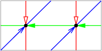
Figure 6.1: Example of a Schnyder wood that has one color whose corresponding subgraph is not connected.

Each connected component of $G_{i}$ has exactly one outgoing edge for each of its vertices. Thus it has exactly one directed cycle that is a monochromatic cycle of color $i$, or $i$-cycle for short. Note that monochromatic cycles can contain edges oriented in two directions with different colors, but the orientation of a $i$-cycle is the orientation given by the (half-)edges of color $i$.

The situation is very different from the plane since the $G_{i}$ are not necessarily connected, contain cycles and we do not have a decomposition into three trees like on Figures 1.6 or 2.3. Nevertheless the behavior of the monochromatic cycles give some interesting global structure.

6.2 Monochromatic cycles

We often use the following lemma that is folklore:

Lemma 26 (Folklore)

Let $C,C^{\prime}$ be two non contractible cycle of a toroidal map. If $C,C^{\prime}$ are not weakly homologous, then their intersection is non empty.

Let $G$ be a toroidal map given with a Schnyder wood. We say that two monochromatic cycles $C_{i},C_{j}$ of different colors are reversal if one is obtained from the other by reversing all the edges, i.e. $C_{i}=C_{j}^{-1}$. We say that two monochromatic cycles are crossing if they intersect but are not reversal. We define the right side of a $i$-cycle $C_{i}$, as the right side while “walking” along the directed cycle by following the orientation given by the edges colored $i$.

Lemma 27

For a given color $i\in\{0,1,2\}$, all $i$-cycles are non-contractible, non intersecting and weakly homologous.

Proof.  By Lemma 6, all $i$-cycles are non-contractible. If there exist two such distinct $i$-cycles that are intersecting, then there is a vertex that has two outgoing edge of color $i$, a contradiction to the Schnyder property. So the $i$-cycles are non intersecting. Then, by Lemma 26, they are weakly homologous. $\Box$

Note that there are Schnyder woods whose $i$-cycles are reversely homologous as shown on the example of Figure 6.2 for which the green color has two cycles going in opposite way.

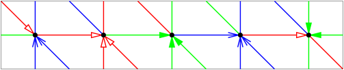
Figure 6.2: Example of a Schnyder wood with some green cycles that are reversely homologous.

Lemma 28

If two monochromatic cycles are crossing then they are not weakly homologous.

Proof.  Suppose that there exist two monochromatic cycles $C_{i-1}$ and $C_{i+1}$, of color $i-1$ and $i+1$, that are crossing and weakly homologous. By Lemma 6, the cycles $C_{i-1}$ and $C_{i+1}$ are non-contractible. Since $C_{i-1}\neq C_{i+1}^{-1}$ and $C_{i-1}\cap C_{i+1}\neq\emptyset$, the cycle $C_{i+1}$ is leaving $C_{i-1}$. It is leaving $C_{i-1}$ on its right side by the Schnyder property. Since $C_{i-1}$ and $C_{i+1}$ are weakly homologous, the cycle $C_{i+1}$ is entering $C_{i-1}$ at least once from its right side, a contradiction to the Schnyder property. $\Box$

Lemma 29

If two monochromatic cycles are intersecting and weakly homologous, then they are reversal.

Proof.  By definition of crossing, two monochromatic cycles that are intersecting, weakly homologous and not reversal contradict Lemma 28. $\Box$

For $i\in\{0,1,2\}$, we define the $i$-winding number $\omega_{i}$ of the Schnyder wood as the number of times a $(i-1)$-cycle crosses a $(i+1)$-cycle. Thus by Lemma 28, we have $\omega_{i}=0$ if the $(i-1)$- and $(i+1)$-cycles are weakly homologous to each other (some may be reversal of each other or not). The winding number of the Schnyder wood is the maximum of the $\omega_{i}$. For example the winding numbers of the Schnyder wood of Figure 6.1 are $\omega_{0}=2$, $\omega_{1}=1$, $\omega_{2}=1$ and those of Figure 6.2 are $\omega_{0}=\omega_{1}=\omega_{2}=0$.

Chapter 7 Crossing Schnyder woods

7.1 Crossing properties

We define properties concerning the way the monochromatic cycles may cross each other. A Schnyder wood of a toroidal map is said to be:

• half-crossing: if there exists a pair $i,j$ of different colors, such that there exist a $i$-cycle crossing a $j$-cycle.

• intersecting: if, for $i\in\{0,1,2\}$, every $i$-cycle intersects at least one $(i-1)$-cycle and at least one $(i+1)$-cycle.

• crossing: if, for $i\in\{0,1,2\}$, every $i$-cycle crosses at least one $(i-1)$-cycle and at least one $(i+1)$-cycle.

The three properties are such that: crossing $\implies$ intersecting $\implies$ half-crossing. The first implication is clear, the second is proved in the following:

Proposition 8

An intersecting Schnyder wood is half-crossing.

Proof.  Consider an $i$-cycle $C_{i}$ that intersects at least one $(i-1)$-cycle $C_{i-1}$ and at least one $(i+1)$-cycle $C_{i+1}$. If $C_{i-1},C_{i},C_{i+1}$ are all weakly homologous, then $C_{i-1}=C_{i}^{-1}=C_{i+1}$ by Lemma 29. This contradicts the definition of Schnyder woods since there is no edges with three colors. So at least two of $C_{i-1},C_{i},C_{i+1}$ are not weakly homologous and thus intersecting by Lemma 26. These two cycles are then crossing. $\Box$

Figures 7.1 gives example of Schnyder woods of a toroidal map that are respectively not half-crossing, half-crossing (and not intersecting), intersecting (and not crossing), crossing.

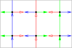
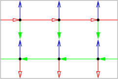
Not half-crossing	Half-crossing
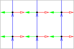
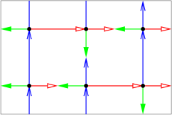
Intersecting	Crossing

Figure 7.1: Example of Schnyder woods of a toroidal map that are respectively not half-crossing, half-crossing, intersecting, crossing.

For triangulation the situation is a bit simpler since ”crossing $\iff$ intersecting”.

Proposition 9

An intersecting Schnyder wood of a toroidal triangulation is crossing.

Proof.  Consider an $i$-cycle $C_{i}$ and a $j$-cycle $C_{j}$ with $i\neq j$. By assumption, cycle $C_{i}$ intersects at least one $j$-cycle $C^{\prime}_{j}$. There is no edges oriented in two directions so $C_{i},C^{\prime}_{j}$ are not reversal of each other. Thus there are not weakly homologous by Lemma 29. By Lemma 27, all the $j$-cycle are weakly homologous. So $C_{i},C_{j}$ are not weakly homologous, thus crossing by Lemma 26. $\Box$

Figure 7.2 gives examples of Schnyder woods of a toroidal triangulation that are respectively not half-crossing, half-crossing (and not crossing), crossing.

Not half-crossing	Half-crossing

Crossing

Figure 7.2: Examples of Schnyder woods of a toroidal triangulation that are respectively not half-crossing, half-crossing, crossing.

The half-crossing property forces the monochromatic cycles to be all homologous and not only weakly homologous as in Lemma 27:

Lemma 30

In a half-crossing Schnyder wood, for $i\in\{0,1,2\}$, all the $i$-cycles are homologous.

Proof.  Consider a half-crossing Schnyder wood. Let $C,C^{\prime}$ be two monochromatic cycles of different colors that are crossing. Let $i\in\{0,1,2\}$. By Lemma 27, all $i$-cycles are weakly homologous. Cycles $C,C^{\prime}$ are not weakly homologous, so at least one of them is not weakly homologous to the $i$-cycles. Assume, w.l.o.g. that $C$ is not weakly homologous to the $i$-cycles. Then by Lemma 26, cycle $C$ crosses all the $i$-cycles. Thus all the $i$-cycles are entering and leaving $C$ from the same sides. So they are all homologous to each other. $\Box$

Consider a toroidal map $G$ given with a Schnyder wood. Let $\mathcal{C}_{i}$ be the set of $i$-cycles of $G$. Let $(\mathcal{C}_{i})^{-1}$ denote the set of cycles obtained by reversing all the cycles of $\mathcal{C}_{i}$.

The following theorem gives a global structure of the monochromatic cycles in the different cases that may occur (see Figure 7.3):

Theorem 9

Let $G$ be a toroidal map given with a Schnyder wood. Then, for $i\in\{0,1,2\}$, all $i$-cycles are non-contractible, non intersecting and weakly homologous. Moreover, if the Schnyder wood is

• Not half-crossing:

  Then all monochromatic cycles are weakly homologous (even if they have different colors).

• Half-crossing:

  Then, for $i\in\{0,1,2\}$, all $i$-cycles are homologous. Moreover there exists a color $i$ such that for any pair of monochromatic cycles $C_{i},C_{j}$ of colors $i,j$, with $i\neq j$, the two cycles $C_{i}$ and $C_{j}$ are crossing (we say that the Schnyder wood is $i$-crossing if we want to specify the color $i$ in this case). Moreover, if the Schnyder wood is:

  • Not crossing:

    Then the $(i-1)$-cycles and the $(i+1)$-cycles are reversely homologous. The Schnyder wood is not $(i-1)$-crossing and not $(i+1)$-crossing. Moreover, if the Schnyder wood is intersecting then $\mathcal{C}_{i-1}=(\mathcal{C}_{i+1})^{-1}$.

  • Crossing:

    Then for every pair of two monochromatic cycles $C_{i},C_{j}$ of different colors $i,j$, the two cycles $C_{i}$ and $C_{j}$ are crossing. The Schnyder wood is $i$-crossing for all $i\in\{0,1,2\}$.

Proof.  By Lemma 27, for a given color $i\in\{0,1,2\}$, all $i$-cycles are non-contractible, non intersecting and weakly homologous. Now we consider the two cases whether the Schnyder wood is half-crossing or not:

• The Schnyder wood is not half-crossing:

  Consider two cycles $C,C^{\prime}$ of distinct colors. Then by definition of half-crossing, $C,C^{\prime}$ are either not intersecting or reversal. If they are not intersecting, they are weakly homologous by Lemma 26, if they are reversal also by definition. So $C,C^{\prime}$ are weakly homologous.

• The Schnyder wood is half-crossing:

  Let $C,C^{\prime}$ be two monochromatic cycles of different colors that are crossing. For $i\in\{0,1,2\}$, by Lemma 27, the $i$-cycles are homologous. Cycles $C,C^{\prime}$ are not weakly homologous, so for all $i\in\{0,1,2\}$, at least one of them is not weakly homologous to the $i$-cycles. There is three value for $i$ and two cycles $C,C^{\prime}$. So there exists $i\in\{0,1,2\}$, such that at least one of $C,C^{\prime}$ is not weakly homologous to all the $(i-1)$-cycles and $(i+1)$-cycles. Assume w.l.o.g. that $C$ satisfies the property. Then by Lemma 26, cycle $C$ intersects, and thus crosses, all the $(i-1)$- and $(i+1)$-cycles. Then $C$ is of color $i$ and all $i$-cycles are homologous to $C$ so they all crosses the $(i-1)$- and $(i+1)$-cycles and the Schnyder wood is $i$-crossing.

  Now we consider the two cases whether the Schnyder wood is crossing or not (we still consider $i$ as above such that the Schnyder wood is $i$-crossing):

  • The Schnyder wood is not crossing:

    Since the Schnyder wood is not crossing there exists two cycles of different colors that are not crossing. None of these cycles are of color $i$ since the Schnyder wood is $i$-crossing. So there exists a $(i-1)$-cycle $C_{i-1}$ and a $(i+1)$-cycle $C_{i+1}$ that are not crossing. If they are intersecting, then they are reversal, and so weakly homologous by definition of crossing. If they are not intersecting, then they are also weakly homologous by Lemma 26. So in both cases, $C_{i-1},C_{i+1}$ are weakly homologous and not crossing. They both crosses a $i$-cycle $C_{i}$, and by the Schnyder property $C_{i-1}$ is crossing $C_{i}$ from left to right, and $C_{i+1}$ is crossing $C_{i}$ from right to left. So $C_{i-1},C_{i+1}$ are reversely homologous, so the $(i-1)$-cycles and the $(i+1)$-cycles are reversely homologous and by Lemma 29. Moreover the Schnyder wood is not $(i-1)$-crossing or $(i+1)$-crossing since $C_{i-1},C_{i+1}$ are not crossing..

    Suppose moreover that the Schnyder wood is intersecting. Let $C^{\prime}_{i-1}$ be any $(i-1)$-cycle. By assumption, $C^{\prime}_{i-1}$ intersects a $(i+1)$-cycle $C^{\prime}_{i+1}$. Cycles $C^{\prime}_{i-1},C^{\prime}_{i+1}$ are reversely homologous. So by Lemma 29, $C^{\prime}_{i-1}$ and $C^{\prime}_{i+1}$ are reversal. Thus $\mathcal{C}_{i-1}\subseteq(\mathcal{C}_{i+1})^{-1}$ and by symmetry $\mathcal{C}_{i-1}=(\mathcal{C}_{i+1})^{-1}$.

  • The Schnyder wood is crossing:

    Since the Schnyder wood is $i$-crossing we just have to prove that $(i-1)$-cycles and $(i+1)$-cycles crosses each other. Consider a $(i-1)$-cycle $C_{i-1}$ and a $(i+1)$-cycle $C_{i+1}$. Cycle $C_{i-1}$ crosses at least one $(i+1)$-cycle $C^{\prime}_{i+1}$. All the $(i+1)$-cycles are homologous to each other so $C_{i-1},C_{i+1}$ are also crossing.

$\Box$

Figure 7.3 illustrates the different case of Theorem 9.

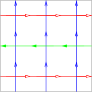
Not half-crossing		Half-crossing
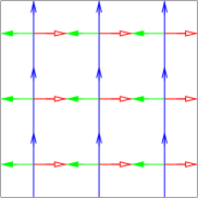
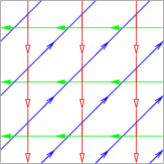
Intersecting		Crossing

Figure 7.3: The global structure of monochromatic cycles in Schnyder woods.

Note that a Schnyder wood that is not half-crossing has winding numbers $\omega_{0}=\omega_{1}=\omega_{2}=0$, a $i$-crossing Schnyder wood that is not crossing has $\omega_{i-1}=\omega_{i+1}=0$, and a crossing Schnyder wood has $\omega_{0}\neq 0,\omega_{1}\neq 0,\omega_{2}\neq 0$.

Half-crossing Schnyder woods are particularly interesting since they enable to define regions in the universal cover, generalizing Figure 2.4, that behave similarly as in the planar case (see Section 7.3).

Half-crossing Schnyder woods of a given toroidal map have the nice property to be all homologous to each other (see Chapter 8), thus they all lie in the same lattice. This lattice behave as a canonical lattice that can be used to obtain interesting bijections (see Chapter 12).

We prove in Chapter 11 that every essentially 3-connected toroidal map admits an intersecting Schnyder wood. In fact, we prove that every essentially 3-connected toroidal map admits a crossing Schnyder wood except for a very simple family of maps depicted on Figure 7.4 (a non-contractible cycle on $n$ vertices, $n\geq 1$, plus $n$ homologous loops).

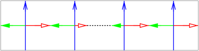
Figure 7.4: The family of basic toroidal maps that admits intersecting Schnyder woods but no crossing Schnyder woods.

Intersecting Schnyder woods, can be used to embed a toroidal map on an orthogonal surfaces and this is particularly interesting for graph drawing purpose (see Chapter 13).

7.2 Crossing and duality

Consider a toroidal map $G$ given with a Schnyder wood. Let $\overline{G}$ be a simultaneous drawing of $G$ and $G^{*}$ such that only dual edges intersect (see example of Figure 7.5).

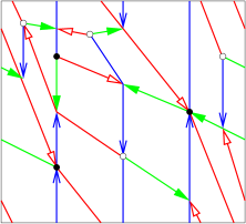
Figure 7.5: Simultaneous drawing of the primal and dual Schnyder wood of Figure 3.12.

The dual of a Schnyder wood is defined in such a way that an edge of $G$ and an edge of $G^{*}$ of the same color never intersect in $\overline{G}$ (see Figure 3.11). Thus the $i$-cycles of $G^{*}$ are weakly homologous to $i$-cycles of $G$. When the Schnyder wood is half-crossing, these cycles are in fact reversely homologous:

Lemma 31

If the Schnyder wood is half-crossing, then, for $i\in\{0,1,2\}$, the $i$-cycles of $G^{*}$ are reversely homologous to the $i$-cycles of $G$.

Proof.  By Theorem 9, there is a color $i$ such that the Schnyder wood is $i$-crossing. Let $C_{i},C_{i+1}$ be a $i$- and $(i+1)$-cycle of $G$. The two cycles $C_{i}$ and $C_{i+1}$ are crossing. Let $j$ be a color in $\{0,1,2\}$. Let $C_{j}$ and $C^{*}_{j}$ be $j$-cycles of the primal and the dual Schnyder wood respectively. Since $C_{i},C_{i+1}$ are crossing, cycle $C_{j}$ is crossing at least one of $C_{i},C_{i+1}$. Since $C^{*}_{j}$ is weakly homologous to $C_{j}$, thus it is crossing the same cycles of $\{C_{i},C_{i+1}\}$ as $C_{j}$ but in opposite direction by the dual rules of Figure 3.11. So $C_{j}$ and $C^{*}_{j}$ are reversely homologous. $\Box$

By Lemma 31, the property of being $i$-crossing thus goes to duality, i.e. a Schnyder wood is $i$-crossing if and only if the dual Schnyder wood is $i$-crossing. Consequently the same is true for the half-crossing and crossing properties by Theorem 9. The intersecting property also goes to duality but this is more difficult to prove. Finally, we have the following:

Proposition 10

A Schnyder wood of a toroidal map is crossing (resp. $i$-crossing, half-crossing, intersecting) if and only if the dual Schnyder wood is crossing (resp. $i$-crossing, half-crossing, intersecting).

Proof.  The result is clear by Theorem 9 and Lemma 31 for crossing, $i$-crossing and half-crossing properties.

Consider now an intersecting Schnyder wood that is not crossing. By Theorem 9 and previous remarks, there is a color $i$ such that the primal and dual Schnyder woods are $i$-crossing. Suppose by contradiction that the dual Schnyder wood is not intersecting. Then there is a $j$-cycle $C^{*}$, with $j\in\{i-1,i+1\}$, that is not intersecting a monochromatic cycle of color in $\{i-1,i+1\}\setminus\{j\}$. By symmetry we can assume that $C^{*}$ is of color $i-1$. By Lemma 31, the $(i-1)$-cycles of $G^{*}$ are reversely homologous to the $(i-1)$-cycles of $G$. Let $C$ be the $(i-1)$-cycle of the primal that is the first on the right side of $C^{*}$ in $\overline{G}$. By Theorem 9, cycle $C^{-1}$ is a $(i+1)$-cycle of $G$. Let $R$ be the region delimited by $C^{*}$ and $C$ situated on the right side of $C^{*}$. Cycle $C^{*}$ is not a $(i+1)$-cycle so there is at least one edge of color $i+1$ leaving a vertex of $C^{*}$. By the Schnyder rule, this edge is entering the interior of the region $R$. An edge of $G^{*}$ of color $i+1$ cannot intersect $C$ and cannot enter $C^{*}$ from its right side. So in the interior of the region $R$ there is at least one $(i+1)$-cycle $C^{*}_{i+1}$ of $G^{*}$. Cycle $C^{*}_{i+1}$ is reversely homologous to $C^{-1}$ by Lemma 31. If $C^{*}_{i+1}$ is not a $(i-1)$-cycle, then we can define $R^{\prime}\subsetneq R$ the region delimited by $C^{*}_{i+1}$ and $C$ situated on the left side of $C^{*}_{i+1}$ and as before we can prove that there is a $(i-1)$-cycle of $G^{*}$ in the interior of $R^{\prime}$. So in any case, there is a $(i-1)$-cycle $C^{*}_{i-1}$ of $G^{*}$ in the interior of $R$ and $C^{*}_{i-1}$ is homologous to $C^{*}$. Let $R^{\prime\prime}\subsetneq R$ be the region delimited by $C^{*}$ and $C^{*}_{i-1}$ situated on the right side of $C^{*}$. Clearly $R^{\prime\prime}$ does not contain $C$. Thus by definition of $C$, the region $R^{\prime\prime}$ does not contain any $(i-1)$-cycle of $G$. But $R^{\prime\prime}$ is non empty and contains at least one vertex $v$ of $G$. The path $P_{i-1}(v)$ cannot leave $R^{\prime\prime}$, a contradiction. So the dual Schnyder wood is intersecting and we have the result. $\Box$

7.3 Crossing in the universal cover

Consider a toroidal map $G$, given with a Schnyder wood. Consider the corresponding orientation and coloring of the edges of the universal cover $G^{\infty}$.

As monochromatic cycles are non-contractible by Theorem 9, a $i$-cycle corresponds to a family of infinite directed monochromatic paths of $G^{\infty}$ (infinite in both directions of the path). These paths are called monochromatic lines of color $i$, or $i$-lines for short. Since all the $i$-cycles are non intersecting and weakly homologous, all the $i$-lines are non intersecting either. The $i$-lines are kind of “parallel” in $G^{\infty}$. Moreover if the Schnyder wood is half-crossing all the $i$-cycles are homologous, so all the $i$-lines are oriented in the same direction.

The definition of $P_{i}(v)$ (defined in Section 3.6) when restricted to the toroidal case is the following: For each color $i$, vertex $v$ is the starting vertex of a infinite path of color $i$, denoted $P_{i}(v)$. By Lemma 7, for every vertex $v$, the three paths $P_{0}(v)$, $P_{1}(v)$, $P_{2}(v)$ are disjoint on all their vertices except on $v$. Thus they divide $G^{\infty}$ into three unbounded regions $R_{0}(v)$, $R_{1}(v)$ and $R_{2}(v)$, where $R_{i}(v)$ denotes the region delimited by the two paths $P_{i-1}(v)$ and $P_{i+1}(v)$ (see Figure 7.6). Let $R_{i}^{\circ}(v)=R_{i}(v)\setminus(P_{i-1}(v)\cup P_{i+1}(v))$. As $P_{i}(v)$ is infinite, it necessarily contains two vertices $u,u^{\prime}$ of $G^{\infty}$ that are copies of the same vertex of $G$. The subpath of $P_{i}(v)$ between $u$ and $u^{\prime}$ corresponds to a $i$-cycle of $G$ and thus is part of a $i$-line of $G^{\infty}$. Let $L_{i}(v)$ be the $i$-line intersecting $P_{i}(v)$.

Figure 7.6: Regions corresponding to a vertex

When the Schnyder wood has the global property of being half-crossing, then it is well structured and the regions $R_{i}(v)$ behave similarly as in the planar case (see [21, 22]):

Lemma 32

If the Schnyder wood is half-crossing, then for all distinct vertices $u$, $v$, we have:

(i)

If $u\in R_{i}(v)$, then $R_{i}(u)\subseteq R_{i}(v)$.

(ii)

If $u\in R_{i}^{\circ}(v)$, then $R_{i}(u)\subsetneq R_{i}(v)$.

(iii)

There exists $i$ and $j$ with $R_{i}(u)\subsetneq R_{i}(v)$ and $R_{j}(v)\subsetneq R_{j}(u)$.

Proof.  (i) Suppose that $u\in R_{i}(v)$. By Theorem 9, there exist $k\in\{0,1,2\}$ such that the Schnyder wood is $k$-crossing. By symmetry we can assume that $k\in\{i-1,i\}$. Then in $G$, $i$-cycles are not weakly homologous to $(i-1)$-cycles. Thus in $G^{\infty}$, every $i$-line crosses every $(i-1)$-line. Moreover a $i$-line crosses a $(i-1)$-line exactly once and from its right side to its left side. Vertex $v$ is between two consecutive monochromatic $(i-1)$-lines $L_{i-1},L^{\prime}_{i-1}$, with $L^{\prime}_{i-1}$ situated on the right of $L_{i-1}$. Let $R$ be the region situated on the right of $L_{i-1}$, so $v\in R$.

Claim 1

For any vertex $w$ of $R$, the path $P_{i}(w)$ leaves the region $R$.

Proof.  The $i$-line $L_{i}(w)$ has to cross $L_{i-1}$ exactly once and from right to left, thus $P_{i}(w)$ leaves the region $R$. $\Diamond$

The paths $P_{i-1}(v)$ and $P_{i+1}(v)$ cannot leave the region $R$ by the Schnyder property. Thus by Claim 1, we have $P_{i}(v)$ leaves the region $R$ and $R_{i}(v)\subseteq R$. So $u\in R$. The paths $P_{i-1}(u)$ and $P_{i+1}(u)$ cannot leave region $R_{i}(v)$. By Claim 1, the path $P_{i}(u)$ leaves the region $R_{i}(v)$ and so $R_{i}(u)\subseteq R_{i}(v)$.

(ii) Suppose that $u\in R_{i}^{\circ}(v)$. By (i), $R_{i}(u)\subseteq R_{i}(v)$. The paths $P_{i-1}(u)$ and $P_{i+1}(u)$ are contained in $R_{i}(v)$ and none of them can contain $v$ by the Schnyder property. So all the faces of $R_{i}(v)$ incident to $v$ are not in $R_{i}(u)$ (and there is at least one such face).

(iii) By symmetry, we prove that there exists $i$ with $R_{i}(u)\subsetneq R_{i}(v)$. If $u\in R_{i}^{\circ}(v)$ for some color $i$, then $R_{i}(u)\subsetneq R_{i}(v)$ by (ii). Suppose now that $u\in P_{i}(v)$ for some $i$. By Lemma 7, at least one of the two paths $P_{i-1}(u)$ and $P_{i+1}(u)$ does no contain $v$. Suppose by symmetry that $P_{i-1}(u)$ does not contain $v$. As $u\in P_{i}(v)\subseteq R_{i+1}(v)$, we have $R_{i+1}(u)\subseteq R_{i+1}(v)$ by (i), and as none of $P_{i-1}(u)$ and $P_{i}(u)$ contains $v$, we have $R_{i+1}(u)\subsetneq R_{i+1}(v)$. $\Box$

Note that if the Schnyder wood is not half-crossing then the conclusions of Lemma 32 might be false. Figure 7.7 gives an example of a Schnyder wood of a toroidal map for which the three items of Lemma 32 are not satisfied. The torus is represented as a black rectangle. It is replicated one time above and one time below to draw partially $G^{\infty}$. The regions $R_{i}(v)$ of the two bold vertices are partially represented by dashed colors. Each bold vertex is in the strict interior of the red region of the other bold vertex but these two vertices do not satisfy any conclusions of the three items of Lemma 32.

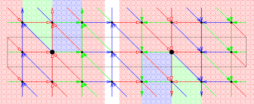
Figure 7.7: Example of a Schnyder wood that is not half-crossing and whose regions do not satisfy the conclusions of Lemma 32.

Chapter 8 Balanced Schnyder woods

8.1 Balanced for maps

In this section we study properties of $\gamma$ and use them to define a particular set of Schnyder woods.

Consider a toroidal map $G$. An $\alpha$-orientation of $\hat{G}$ is called a $3$-orientation if:

$$\alpha(v)=\begin{cases}3&\text{if }v\text{ is a primal- or dual-vertex},\\ 1&\text{if }v\text{ is an edge-vertex.}\\ \end{cases}$$

Next lemma shows that $\gamma$ behaves well w.r.t. homologous cycles in $3$-orientations of $\hat{G}$: two homologous non-contractible cycles have the same value $\gamma$. We formulate this in a more general form:

Lemma 33

Consider a $3$-orientation of $\hat{G}$, a non-contractible cycle $C$ of $G$ or $G^{*}$, given with a direction of traversal, and a homology-basis $\{B_{1},B_{2}\}$ of $G$, such that $B_{1},B_{2}$ are non-contractible cycles whose intersection is a single vertex or a common path. If $\hat{C}$ is homologous to $k_{1}\hat{B_{1}}+k_{2}\hat{B_{2}}$, with $k_{1},k_{2}\in\mathbb{Z}$, then $\gamma(C)=k_{1}\,\gamma(B_{1})+k_{2}\,\gamma(B_{2})$.

Proof.  Let $v$ be a vertex in the intersection of $B_{1},B_{2}$ such that, if this intersection is a common path, then $v$ is one of the extremities of this path and let $u$ be the other extremity. Consider a drawing of $(\hat{G})^{\infty}$ obtained by replicating a flat representation of $\hat{G}$ to tile the plane. Let $v_{0}$ be a copy of $v$ in $(\hat{G})^{\infty}$. Consider the walk $W$ starting from $v_{0}$ and following $k_{1}$ times the edges corresponding to $B_{1}$ and then $k_{2}$ times the edges corresponding to $B_{2}$ (we are going backward if $k_{i}$ is negative). This walk ends at a copy $v_{1}$ of $v$. Since $C$ is non-contractible we have $k_{1}$ or $k_{2}$ not equal to $0$ and thus $v_{1}$ is distinct from $v_{0}$. Let $W^{\infty}$ be the infinite walk obtained by replicating $W$ (forward and backward) from $v_{0}$. Note that their might be some repetition of vertices in $W^{\infty}$ if the intersection of $B_{1},B_{2}$ is a path. But in that case, by the choice of $B_{1},B_{2}$, we have that $W^{\infty}$ is almost a path, except maybe at all the transitions from “$k_{1}{B_{1}}$” to “$k_{2}B_{2}$”, or at all the transitions from “$k_{2}{B_{2}}$” to “$k_{1}B_{1}$”, where it can goes back and forth a path corresponding to the intersection of $B_{1}$ and $B_{2}$. The existence or not of such “back and forth” parts depends on the signs of $k_{1},k_{2}$ and the way $B_{1},B_{2}$ are going through their common path. Figure 8.2 gives an example of this construction with $(k_{1},k_{2})=(1,1)$ and $(k_{1},k_{2})=(1,-1)$ when $B_{1},B_{2}$ intersects on a path and are oriented the same way along this path as on Figure 8.1.

Figure 8.1: Intersection of the basis.

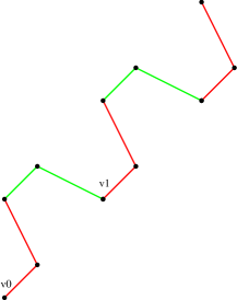
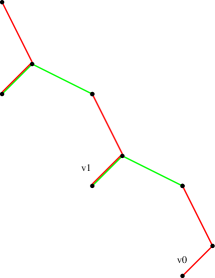
$(k_{1},k_{2})=(1,1)$	$(k_{1},k_{2})=(1,-1)$

Figure 8.2: Replicating “$k_{1}{B_{1}}$” and “$k_{2}B_{2}$” in the universal cover.

We “simplify” $W^{\infty}$ by removing all the parts that consists of going back and forth along a path (if any) and call $B^{\infty}$ the obtained walk that is now without repetition of vertices. By the choice of $v$, we have that $B^{\infty}$ goes through copies of $v$. If $v_{0},v_{1}$ are no more a vertex along $B^{\infty}$, because of a simplification at the transition from “$k_{2}{B_{2}}$” to “$k_{1}B_{1}$”, then we replace $v_{0}$ and $v_{1}$ by the next copies of $v$ along $W^{\infty}$, i.e. at the transition from “$k_{1}{B_{1}}$” to “$k_{2}B_{2}$”.

Since $\hat{C}$ is homologous to $k_{1}\hat{B_{1}}+k_{2}\hat{B_{2}}$, we can find an infinite path $C^{\infty}$, that corresponds to copies of $C$ replicated, that does not intersect $B^{\infty}$ and situated on the right side of $B^{\infty}$. Now we can find a copy $B^{\prime\infty}$ of $B^{\infty}$, such that $C^{\infty}$ lies between $B^{\infty}$ and $B^{\prime\infty}$ without intersecting them. Choose two copies $v^{\prime}_{0},v^{\prime}_{1}$ of $v_{0},v_{1}$ on $B^{\prime\infty}$ such that the vectors $v_{0}v_{1}$ and $v^{\prime}_{0}v^{\prime}_{1}$ are equal.

Let $R_{0}$ be the region bounded by $B^{\infty},B^{\prime\infty}$. Let $R_{1}$ (resp. $R_{2}$) be the subregion of $R_{0}$ delimited by $B^{\infty}$ and $C^{\infty}$ (resp. by $C^{\infty}$ and $B^{\prime\infty}$). We consider $R_{0},R_{1},R_{2}$ as cylinders, where the segments $[v_{0},v^{\prime}_{0}],[v_{1},v_{1}^{\prime}]$ (or part of them) are identified. Let $B,B^{\prime},C^{\prime}$ be the cycles of $R_{0}$ corresponding to $B^{\infty},B^{\prime\infty},C^{\prime\infty}$ respectively. Let $x$ be the number of edges of $\hat{G}$ leaving $B$ in $R_{1}$. Let $y$ be the number of edges of $\hat{G}$ leaving $B^{\prime}$ in $R_{2}$. Let $x^{\prime}$ (resp. $y^{\prime}$) be the number of edges of $\hat{G}$ leaving $C^{\prime}$ in $R_{2}$ (resp. $R_{1}$). We have $C^{\prime}$ corresponds to exactly one copy of $C$, so $\gamma(C)=x^{\prime}-y^{\prime}$. Similarly, we have $B$ and $B^{\prime}$ that almost corresponds to $k_{1}$ copies of $B_{1}$ followed by $k_{2}$ copies of $B_{2}$, except the fact that we may have removed a back and forth part (if any). In any case we have the following:

Claim 2

$k_{1}\,\gamma(B_{1})+k_{2}\,\gamma(B_{2})=x-y$

Proof.  We prove the case where the common intersection of $B_{1},B_{2}$ is a path (if the intersection is a single vertex, the proof is very similar and even simpler). We assume, w.l.o.g, by eventually reversing one of $B_{1}$ or $B_{2}$, that $B_{1},B_{2}$ are oriented the same way along their intersection, so we are in the situation of Figure 8.1.

Figure 8.3 shows how to compute $k_{1}\,\gamma(B_{1})+k_{2}\,\gamma(B_{2})+y-x$ when $(k_{1},k_{2})=(1,1)$. Then, one can check that each outgoing edge of $\hat{G}$ is counted exactly the same number of time positively and negatively. So everything compensate and we obtain $k_{1}\,\gamma(B_{1})+k_{2}\,\gamma(B_{2})+y-x=0$.

$\gamma(B_{1})$	$+$	$\gamma(B_{2})$	$+$	$(y-x)$	$=0$

Figure 8.3: Case $(k_{1},k_{2})=(1,1)$.

Figure 8.4 shows how to compute $k_{1}\,\gamma(B_{1})+k_{2}\,\gamma(B_{2})+y-x$ when $(k_{1},k_{2})=(1,-1)$. As above, most of the things compensate but, in the end, we obtain $k_{1}\,\gamma(B_{1})+k_{2}\,\gamma(B_{2})+y-x=d^{+}(u)-d^{+}(v)$, as depicted on the figure. Since the number of outgoing edges around each vertex is equal to $3$, we have again the conclusion $k_{1}\,\gamma(B_{1})+k_{2}\,\gamma(B_{2})+y-x=0$.

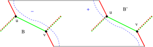
$\gamma(B_{1})$	$+$	$(-\gamma(B_{2}))$	$+$	$(y-x)$

$=d^{+}(u)-d^{+}(v)=0$

Figure 8.4: Case $(k_{1},k_{2})=(1,-1)$..

One can easily be convinced that when $|k_{1}|\geq 1$ and $|k_{2}|\geq 1$ then the same arguments apply. The only difference is that the red or green part of the figures in the universal cover would be longer (with repetitions of $B_{1}$ and $B_{2}$). This parts being very “clean”, they do not affect the way we compute the equality. Finally, if one of $k_{1}$ or $k_{2}$ is equal to zero, the analysis is much simpler and the conclusion holds. $\Diamond$

For $i\in\{1,2\}$, let $H_{i}$ be the cylinder map made of all the vertices and edges of $\hat{G}^{\infty}$ that are in the cylinder region $R_{i}$. Let $k$ (resp. $k^{\prime}$) be the length of $B$ (resp. $C^{\prime}$). Let $n_{1},m_{1},f_{1}$ be respectively the number of vertices, edges and faces of $H_{1}$. Let $n_{pd}$ be the number of primal- and dual-vertices of $H_{1}$ and $n_{e}$ be its number of edge-vertices. We have $n_{1}=n_{pd}+n_{e}$. Since $H_{1}$ is a quadrangulation we have $4f_{1}=2m_{1}-2(k+k^{\prime})$. Each edge of $H_{1}$ is incident to an edge-vertex. All the edge-vertices of $H_{1}$ have degree $4$ except those that are on $B$ and $C^{\prime}$ that have degree $3$, so the total number of edges of $H_{1}$ is $m_{1}=4n_{e}-(k+k^{\prime})$. Finally combining these equalities with Euler’s formula $n_{1}-m_{1}+f_{1}=0$, one obtain that $n_{pd}=n_{e}$. Moreover, since we are considering a $3$-orientation of $\hat{G}$, we have that $m_{1}=3n_{pd}+n_{e}-(x^{\prime}+y)=4n_{e}-(x^{\prime}+y)$. So finally, by combining this with above formula, we obtain $k+k^{\prime}=x^{\prime}+y$. Similarly, by considering $H_{2}$, one obtain that $k+k^{\prime}=x+y^{\prime}$. Thus finally $x^{\prime}+y=x+y^{\prime}$ and thus $\gamma(C)=k_{1}\,\gamma(B_{1})+k_{2}\,\gamma(B_{2})$ by Claim 2. $\Box$

Recall from Section 5.1 that, given a homology-basis of $G$ formed by a pair of cycles $B_{1},B_{2}$ of $G$, the type of a 3-orientation of $\hat{G}$ is $\Gamma=(\gamma(B_{1}),\gamma(B_{2}))$. Lemma 33 implies the following:

Lemma 34

In a 3-orientation $D$ of $\hat{G}$ the following are equivalent:

1. For two non-contractible not weakly homologous cycles $C,C^{\prime}$ of ${G}$, we have $\gamma(C)=\gamma(C^{\prime})=0$.

2. $D$ has type $(0,0)$ for a homology-basis of $G$ formed by a pair of cycles.

3. $D$ has type $(0,0)$ for any homology-basis of $G$ formed by a pair of cycles.

4. For any non-contractible cycle $C$ of ${G}$ or $G^{*}$, we have $\gamma(C)=0$.

Proof.  Clearly $4.\Longrightarrow 3.\Longrightarrow 2.\Longrightarrow 1.$.

We now prove that $1.\Longrightarrow 4.$ is implied by Lemma 33. Consider two non-contractible not weakly homologous cycles $C,C^{\prime}$ of ${G}$ such that $\gamma(C)=\gamma(C^{\prime})=0$. Consider an homology-basis $\{B_{1},B_{2}\}$ of $G$, such that $B_{1},B_{2}$ are non-contractible cycles whose intersection is a single vertex or a path (see Section 4.1 for discussion on existence of such a basis). Let $k_{1},k_{2},k^{\prime}_{1},k^{\prime}_{2}\in\mathbb{Z}$, such that $C$ (resp. $C^{\prime}$) is homologous to $k_{1}B_{1}+k_{2}B_{2}$ (resp. $k^{\prime}_{1}B_{1}+k^{\prime}_{2}B_{2}$). Since $C$ is non-contractible we have $(k_{1},k_{2})\neq(0,0)$. By eventually exchanging $B_{1},B_{2}$, we can assume, w.l.o.g., that $k_{1}\neq 0$. By Lemma 33, we have $k_{1}\gamma(B_{1})+k_{2}\gamma(B_{2})=\gamma(C)=0=\gamma(C^{\prime})=k^{\prime}_{1}\gamma(B_{1})+k^{\prime}_{2}\gamma(B_{2})$. So $\gamma(B_{1})=(-k_{2}/k_{1})\gamma(B_{2})$ and thus $(-k_{2}k^{\prime}_{1}/k_{1}+k^{\prime}_{2})\gamma(B_{2})=0$. So $k^{\prime}_{2}=k_{2}k^{\prime}_{1}/k_{1}$ or $\gamma(B_{2})=0$. Suppose by contradiction, that $\gamma(B_{2})\neq 0$. Then $(k^{\prime}_{1},k^{\prime}_{2})=\frac{k^{\prime}_{1}}{k_{1}}(k_{1},k_{2})$, and $C^{\prime}$ is homologous to $\frac{k^{\prime}_{1}}{k_{1}}C$. Since $C$ and $C^{\prime}$ are both non-contractible cycles, it is not possible that one is homologous to a multiple of the other, with a multiple different from $-1,1$. So $C,C^{\prime}$ are weakly homologous, a contradiction. So $\gamma(B_{2})=0$ and thus $\gamma(B_{1})=0$. Then by Lemma 33, any non-contractible cycle of ${G}$ or $G^{*}$, have $\gamma$ equal to $0$. $\Box$

Consider a homology-basis of $G$ that is formed by a pair of cycles of $G$. We define the set $S_{0}(\hat{G})$ of all the $3$-orientations of $\hat{G}$ that have type $\Gamma=(0,0)$ in the considered basis. By Lemma 34, the definition of $S_{0}(\hat{G})$ does not depend on the choice of the basis, so its element form a kind of canonical set. We call the elements of $S_{0}(\hat{G})$ balanced orientations. A $3$-orientation of $\hat{G}$ is a balanced orientation if and only if it satisfies any condition of Lemma 34. By Theorem 5, balanced orientations are homologous to each other. By Theorem 8, they carry a structure of distributive lattice. This special lattice acts as a canonical lattice and this is particularly important for bijection purpose (see Chapter 12). By Theorem 4, balanced orientations corresponds to Schnyder woods of $G$ that we call balanced Schnyder woods. By Lemma 34, a Schnyder wood is balanced if and only if the dual Schnyder wood is balanced.

Note that there exists Schnyder woods that are not balanced. The Schnyder wood of Figure 8.5 is an example where the horizontal cycle has $\gamma$ equal to $\pm 6$. Thus it is not balanced by Lemma 34.

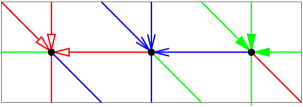
Figure 8.5: A Schnyder wood of a toroidal triangulation that is not balanced.

One can remark that on Figure 8.5, the three monochromatic cycles are all homologous to each other (i.e. going in the same direction). In fact this is a general property that can be proved: a Schnyder wood that is not balanced has three monochromatic cycles of different colors that are all homologous to each other.

Note that this property does not give a characterization of Schnyder woods that are not balanced. Figure 8.6 is an example of a balanced Schnyder wood with three monochromatic cycles of different colors that are homologous. The value of $\gamma$ for the horizontal and a vertical cycle is $0$, thus it is balanced.

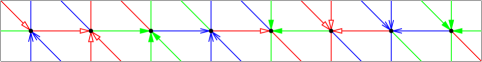
Figure 8.6: Example of a balanced Schnyder wood with three monochromatic cycles of different colors that are homologous.

8.2 Balanced vs crossing

Consider a toroidal map $G$. Function $\gamma$ behaves well with Schnyder woods of $G$ since monochromatic cycles have $\gamma$ equals to zero:

Lemma 35

In a Schnyder wood of $G$, a monochromatic cycle $C$ of $G$ satisfies $\gamma(C)=0$.

Proof.  We consider a $i$-cycle $C$ of $G$ and its corresponding cycle $\hat{C}$ in $\hat{G}$. Thus $\hat{C}$ is alternating primal- and edge-vertices and in the direction of traversal of $C$, all the edges after a primal-vertex are outgoing and of color $i$. Let $u,v,w$ be three consecutive vertices of $C$, and $x,y$ be the edge-vertices between them in $\hat{C}$, so $u,x,v,y,w$ appear in this order along $\hat{C}$. The edges $e=ux$ and $e^{\prime}=vy$ are outgoing for $u$ and $v$ and of color $i$. We consider three cases depending on the possible orientation and coloring of edge $xv$. These cases are represented on Figure 8.7. One can check that in each case the computation of $\gamma$ on the part of $C$ between $e$ and $e^{\prime}$ is equal to $0$. Thus in total we have $\gamma(C)=0$. $\Box$

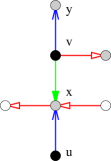
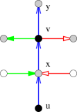
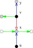
Figure 8.7: The three cases that can occur when considering a part of a monochromatic cycle (vertical edges on the figure).

Lemma 35 implies the following:

Proposition 11

an half-crossing Schnyder wood of $G$ is balanced.

Proof.  Suppose that the Schnyder wood is $i$-crossing by Theorem 9. Let $C_{i},C_{i-1}$ be two crossing monochromatic cycles of color $i$ and $i-1$ respectively. Cycles $C_{i}$ and $C_{i-1}$ are non-contractible, not weakly homologous and satisfy $\gamma(C_{i})=\gamma(C_{i-1})=0$ by Lemma 35. So by Lemma 34, the Schnyder wood is balanced. $\Box$

By Proposition 11, the set of balanced Schnyder woods contains all the half-crossing Schnyder woods but it may also contain some Schnyder woods that are not half-crossing. The Schnyder wood of Figure 8.8 is an example where $\gamma(C)=0$ for any non-contractible cycle $C$ of $G$, so it is balanced. It is not half-crossing since all the monochromatic cycles are weakly homologous (vertical on the figure).

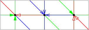
Figure 8.8: A Schnyder wood of a toroidal triangulation that is balanced and not half-crossing.

8.3 Balanced for triangulations

Consider a toroidal triangulation $G$ given with an orientation. Recall that the edges of the dual $G^{*}$ of $G$ are oriented such that the dual $e^{*}$ of an edge $e$ of $G$ goes from the face on the right of $e$ to the face on the left of $e$. (We insist that we do not consider duality of Schnyder woods here but just a convention of orientation of edges of $G^{*}$.)

Lemma 36

Consider an orientation of $G$ corresponding to a balanced Schnyder wood, then the dual orientation of $G^{*}$ contains no oriented non-contractible cycle.

Proof.  Suppose by contradiction that there exists an oriented non-contractible cycle $C$ is the dual orientation. We compute $\gamma(C)$ to obtain a contradiction. Since $C$ is an oriented cycle in the dual, all the edges of $\hat{G}$ that are incident to edge-vertices of $\hat{C}$ and on the right of $\hat{C}$ are outgoing and each of them counts $+1$ for $\gamma$. All the edges of $\hat{G}$ that are incident to edge-vertices of $\hat{C}$ and on the left of $\hat{C}$ are ingoing and count $0$ for $\gamma$. So each edge-vertex of $\hat{C}$ counts $+1$ for $\gamma$. Since we are considering a triangulation, all the edges of $\hat{G}$ incident to dual-vertices of $\hat{C}$ are outgoing. Moreover each dual-vertex of $\hat{C}$ is incident to exactly one such edge that is not on $\hat{C}$. Since $C$ is non-contractible, there is at least one edge incident to a dual-vertex of $\hat{C}$ and on the right side of $\hat{C}$. This edge counts $+1$ for $\gamma$. Since $\hat{C}$ has the same number $k$ of dual- and edge-vertices, we have $\gamma(C)\geq k+1-(k-1)=2$, a contradiction to Lemma 34. $\Box$

Lemma 36 gives the key property of balanced Schnyder woods in triangulations that enables to generalize Poulalhon and Schaeffer’s method [45] for the toroidal case, as done in Chapter 12.

For the non-balanced Schnyder wood of Figure 8.5, one can see that there is an horizontal oriented non-contractible cycle in the dual, so it does not satisfy the conclusion of Lemma 36. Note that the conclusion of Lemma 36 is not a characterization of being balanced. Figure 8.9 gives an example of a Schnyder wood that is not balanced but satisfies the conclusion of Lemma 36 (its horizontal cycle has $\gamma$ equals $\pm 6$).

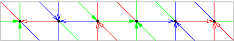
Figure 8.9: A Schnyder wood that is not balanced but contains no oriented non-contractible cycle in the dual.

8.4 Balanced lattice for triangulations

In this section, we push further the study of the lattice of balanced Schnyder woods for triangulations. These properties are used in Chapter 12 to obtain a nice bijection.

Consider a toroidal triangulation $G$ and suppose that $G$ admits a balanced orientation, so $S_{0}({G})$ is non-empty. An $\alpha$-orientation of $G$ is called a $3$-orientation if $\alpha(v)=3$ for all vertices $v$ of $G$. Recall that $S_{0}(\hat{G})$ denotes the set of all balanced orientations of $\hat{G}$. Since we are considering a triangulation, the $3$-orientations of $G$ are in bijection with the $3$-orientation of $\hat{G}$. Thus we simply denote $S_{0}({G})$ the $3$-orientations of $G$ corresponding to elements of $S_{0}(\hat{G})$. Let $f_{0}$ be any face of $G$. By Theorem 8, we have that $(S_{0}({G}),\leq_{f_{0}})$ is a distributive lattice. Let $\widetilde{G}$ be the graph obtained from $G$ by deleting all the rigid edges of $G$, i.e. edges that have the same orientation in all elements of $S_{0}({G})$ (see Section 5.2).

Suppose that $G$ is given with a 3-orientation. For an edge $e_{0}$ of $G$ we define the left walk from $e_{0}$ as the sequence of edges $W=(e_{i})_{i\geq 0}$ of $G$ obtained by the following: if the edge $e_{i}$ is entering a vertex $v$, then $e_{i+1}$ is chosen among the three edges leaving $v$ as the edge that is on the left coming from $e_{i}$ (i.e. the first one while going clockwise around $v$). A closed left-walk is left walk that is repeating periodically on itself, i.e. a finite sequence of edges $W=(e_{i})_{0\leq i\leq k-1}$ such that its repetition is a left-walk. We have the following lemma concerning closed left-walks in balanced orientations:

Lemma 37

In an orientation $D$ of $S_{0}(G)$, a closed left walk $W$ of $G$ is a triangle with its interior on its left side.

Proof.  Consider a closed left walk $W=(e_{i})_{0\leq i\leq k-1}$ of $D$, with $k\geq 1$. W.l.o.g., we may assume that all the $e_{i}$ are distinct, i.e. there is no strict subwalk of $W$ that is also a closed left walk. Note that $W$ cannot cross itself otherwise it is not a left walk. However $W$ may have repeated vertices but in that case it intersects itself tangentially on the right side.

Suppose by contradiction that there is an oriented subwalk $W^{\prime}$ of $W$, that forms a cycle $C$ enclosing a region $R$ on its right side that is homeomorphic to an open disk. Let $v$ be the starting and ending vertex of $W^{\prime}$. Note that we do not consider that $W^{\prime}$ is a strict subwalk of $W$, so we might have $W^{\prime}=W$. Consider the graph $G^{\prime}$ obtained from $G$ by keeping all the vertices and edges that lie in the region $R$, including $W^{\prime}$. Since $W$ can intersect itself only tangentially on the right side, we have that $G^{\prime}$ is a plane map whose outer face boundary is $W^{\prime}$ and whose interior is triangulated. Let $k^{\prime}$ be the length of $W^{\prime}$. Let $n^{\prime},m^{\prime},f^{\prime}$ be the number of vertices, edges and faces of $G^{\prime}$. By Euler’s formula, $n^{\prime}-m^{\prime}+f^{\prime}=2$. All the inner faces have size $3$ and the outer face has size $k^{\prime}$, so $2m^{\prime}=3(f^{\prime}-1)+k^{\prime}$. Since $W^{\prime}$ is a subwalk of a left walk, all the vertices of $G^{\prime}$, except $v$, have their outgoing edges in $G^{\prime}$. Since $W^{\prime}$ is following oriented edges of $G$, vertex $v$ has at least one outgoing edge in $G^{\prime}$. Thus, as we are considering a $3$-orientation, we have $m^{\prime}\geq 3(n^{\prime}-1)+1$. Combining these three equalities gives $k^{\prime}\leq-1$, a contradiction. So there is no oriented subwalk of $W$, that forms a cycle enclosing an open disk on its right side.

We now claim the following:

Claim 3

The left side of $W$ encloses a region homeomorphic to an open disk

Proof.  We consider two cases depending on the fact that $W$ is a cycle (i.e. with no repetition of vertices) or not.

• $W$ is a cycle

  Suppose by contradiction that $W$ is a non-contractible cycle. We have $k$ is the length of $W$. Since we are considering a $3$-orientation, the total number of outgoing edges incident to vertices of $W$ is $3k$. There are $k$ such edges that are on $W$. Since $W$ is a left walk, there is no outgoing edge incident to its left side. So there are $2k$ outgoing edges incident to its right side. Thus $\gamma(W)=2k\neq 0$. So by Lemma 34, the $3$-orientation $D$ is not balanced, a contradiction. Thus $W$ is a contractible cycle. As explained above, the contractible cycle $W$ does not enclose a region homeomorphic to an open disk on its right side. So $W$ encloses a region homeomorphic to an open disk on its left side, as claimed.

• $W$ is not a cycle

  Since $W$ cannot cross itself nor intersect itself tangentially on the left side, it has to intersect tangentially on the right side. Such an intersection on a vertex $v$ is depicted on Figure 8.10.(a). The edges of $W$ incident to $v$ are noted as on the figure, $a,b,c,d$, where $W$ is going periodically trough $a,b,c,d$ in this order. The (green) subwalk of $W$ from $a$ to $b$ does not enclose a region homeomorphic to an open disk on its right side. So we are not in the case depicted on Figure 8.10.(b). Moreover if this (green) subwalk encloses a region homeomorphic to an open disk on its left side, then this region contains the (red) subwalk of $W$ from $c$ to $d$, see Figure 8.10.(c). Since $W$ cannot cross itself, this (red) subwalk necessarily encloses a region homeomorphic to an open disk on its right side, a contradiction. So the (green) subwalk of $W$ starting from $a$ has to form a non-contractible curve before reaching $b$. Similarly for the (red) subwalk starting from $c$ and reaching $d$. Since $W$ is a left-walk and cannot cross itself, we are, w.l.o.g., in the situation of Figure 8.10.(d) (with possibly more tangent intersections on the right side). In any case, the left side of $W$ encloses a region homeomorphic to an open disk.

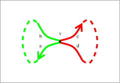
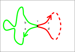
  (a)	(b)
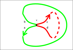
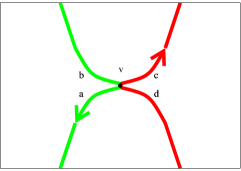
  (c)	(d)

  Figure 8.10: Case analysis for the proof of Claim 3.

$\Diamond$

By Claim 3, the left side of $W$ encloses a region $R$ homeomorphic to an open disk. Consider the graph $G^{\prime}$ obtained from $G$ by keeping only the vertices and edges that lie in the region $R$, including $W$. The vertices of $W$ appearing several times are duplicated so that $G^{\prime}$ is a plane triangulation of a cycle. Let $n^{\prime},m^{\prime},f^{\prime}$ be the number of vertices, edges and faces of $G^{\prime}$. By Euler’s formula, $n^{\prime}-m^{\prime}+f^{\prime}=2$. All the inner faces have size $3$ and the outer face has size $k$, so $2m^{\prime}=3(f^{\prime}-1)+k$. All the inner vertices have outdegree $3$ as we are considering a $3$-orientation of $G$. All the inner edges of $G^{\prime}$ incident to $W$ are oriented toward $W$, and there are $k$ outer edges, so $m^{\prime}=3(n^{\prime}-k)+k$. Combining these three equalities gives $k=3$, i.e. $W$ has size three and the lemma holds. $\Box$

The boundary of a face of $\widetilde{G}$ may be composed of several closed walks. Let us call quasi-contractible the faces of $\widetilde{G}$ that are homeomorphic to an open disk or to an open disk with punctures. Note that such a face may have several boundaries (if there are some punctures) but exactly one of these boundaries encloses the face. Let us call outer facial walk this special boundary. Then we have the following:

Lemma 38

All the faces of $\widetilde{G}$ are quasi-contractible and their outer facial walk is a triangle.

Proof.  Suppose by contradiction that there is a face $\widetilde{f}$ of $\widetilde{G}$ that is not quasi-contractible or that is quasi-contractible but whose outer facial walk is not a triangle. Let $\widetilde{F}$ be the element of $\widetilde{\mathcal{F}}$ corresponding to the boundary of $\widetilde{f}$. By Lemma 23, there exists an orientation $D$ in $S_{0}(G)$ such that $\widetilde{F}$ is an oriented subgraph of $D$.

All the faces of $G$ are triangles. Thus $\widetilde{f}$ is not a face of $G$ and contains in its interior at least one edge of $G$. Start from any such edge $e_{0}$ and consider the left walk $W=(e_{i})_{i\geq 0}$ of $D$ from $e_{0}$. Suppose that for $i\geq 0$, edge $e_{i}$ is entering a vertex $v$ that is on the border of $\widetilde{f}$. Recall that by definition $\widetilde{F}$ is oriented counterclockwise according to its interior, so either $e_{i+1}$ is in the interior of $\widetilde{f}$ or $e_{i+1}$ is on the border of $\widetilde{f}$. Thus $W$ cannot leave $\widetilde{f}$.

Since $G$ has a finite number of edges, some edges are used several times in $W$. Consider a minimal subsequence $W^{\prime}=e_{k},\ldots,e_{\ell}$ such that no edge appears twice and $e_{k}=e_{\ell+1}$. Thus $W$ ends periodically on $W^{\prime}$ that is a closed left walk. By Lemma 37, $W^{\prime}$ is a triangle with its interior $R$ on its left side. Thus $W^{\prime}$ is a $0$-homologous oriented subgraph of $D$. So all its edges are non-rigid by Lemma 20. So all the edges of $W^{\prime}$ are part of the border of $\widetilde{f}$. Since $\widetilde{F}$ is oriented counterclockwise according to its interior, the region $R$ contains $\widetilde{f}$. So $\widetilde{f}$ is quasi-contractible and $W^{\prime}$ is its outer facial walk and a triangle, a contradiction. $\Box$

By Lemma 38, every face of $\widetilde{G}$ is quasi-contractible and its outer facial walk is a triangle. So $\widetilde{G}$ contains all the triangles of $G$ whose interiors are maximal by inclusion, i.e. it contains all the edges that are not in the interior of a separating triangle. In particular, $\widetilde{G}$ is non-empty and $|S_{0}(G)|\geq 2$. The status (rigid or not) of an edge lying inside a separating triangle is determined as in the planar case: such an edge is rigid if and only if it is in the interior of a separating triangle and incident to this triangle. Thus an edge of $G$ is rigid if and only if it is in the interior of a separating triangle and incident to this triangle.

Since $(S_{0}(G),\leq_{f_{0}})$ is a distributive lattice, any element $D$ of $S_{0}(G)$ that is distinct from $D_{\max}$ and $D_{\min}$ contains at least one neighbor above and at least one neighbor below in the Hasse diagram of the lattice. Thus it has at least one face of $\widetilde{G}$ oriented counterclockwise and at least one face of $\widetilde{G}$ oriented clockwise. Thus by Lemma 38, it contains at least one triangle oriented counterclockwise and at least one triangle oriented clockwise. Next lemma shows that this property is also true for $D_{\max}$ and $D_{\min}$.

Lemma 39

In $D_{\max}$ (resp. $D_{\min}$) there is a counterclockwise (resp. clockwise) triangle containing $f_{0}$, and a clockwise (resp. counterclockwise) triangle not containing $f_{0}$.

Proof.  By Lemma 38, $\widetilde{f}_{0}$ is quasi-contractible and its outer facial walk is a triangle $T$. By Lemma 24, $\widetilde{F}_{0}$ is an oriented subgraph of $D_{\max}$. Thus $T$ is oriented counterclockwise and contains $f_{0}$. The second part of the lemma is clear since $|S_{0}(G)|\geq 2$ so $D_{\max}$ has at least one neighbor below in the Hasse diagram of the lattice. Similarly for $D_{\min}$. $\Box$

Thus by above remarks and Lemma 39, all the balanced Schnyder woods have at least one triangle oriented counterclockwise and at least one triangle oriented clockwise. Note that this property does not characterize balanced Schnyder woods. Figure 8.9 gives an example of a Schnyder wood that is not balanced but satisfies the property. Note also that not all Schnyder woods satisfy the property. Figure 8.5 is an example of a Schnyder wood that is not balanced and has no oriented triangle.

Chapter 9 Example of a balanced lattice

Figure 9.1 illustrates the Hasse diagram of the balanced Schnyder woods of the toroidal triangulation $G$ of Figure 8.8. Bold black edges are the edges of the Hasse diagram $\mathcal{H}$. Each node of the diagram is a balanced Schnyder wood of $G$. In every Schnyder wood, a face is dotted if its boundary is directed. In the case of the special face $f_{0}$ the dot is black. Otherwise, the dot is magenta if the boundary cycle is oriented counterclockwise and cyan otherwise. An edge in the Hasse diagram from $D$ to $D^{\prime}$ (with $D\leq D^{\prime}$) corresponds to a face oriented counterclockwise in $D$ whose edges are reversed to form a face oriented clockwise in $D^{\prime}$, i.e. a magenta dot is replaced by a cyan dot. The outdegree of a node is its number of magenta dots and its indegree is its number of cyan dots. All edges are not in the interior of a triangle, so, by previous section, they are not rigid. By Lemma 23, all the faces have a dot at least once. The special face is not allowed to be flipped, it is oriented counterclockwise in the maximal Schnyder wood and clockwise in the minimal Schnyder wood by Lemma 24. By Lemma 25, the maximal (resp. minimal) Schnyder wood contains no other faces oriented counterclockwise (resp. clockwise), indeed it contains only cyan (resp. magenta) dots. The words “no”, “half”, “full” correspond to Schnyder woods that are not half-crossing, half-crossing (but not crossing), and crossing, respectively. By Proposition 11, the diagram contains all the half-crossing Schnyder woods of $G$. The minimal element is the Schnyder wood of Figure 8.8, and its neighbor is the half-crossing Schnyder wood of Figure 7.2.

In the example the two crossing Schnyder woods lie in the “middle” of the lattice. These Schnyder woods are of particular interests for graph drawing purpose (see Chapter 13) whereas the minimal balanced Schnyder wood (not crossing in this example) is important for bijective encoding (see Chapter 12). We show in next section how to find in linear time either a minimal balanced Schnyder wood or a crossing Schnyder wood in the case of toroidal triangulations.

Figure 9.1: Example of the Hasse diagram of the distributive lattice of homologous orientations of a toroidal triangulation.

The underlying toroidal triangulation of Figure 9.1 has only two Schnyder woods not depicted in Figure 9.1. One of them two Schnyder wood is shown in Figure 8.5 and the other one is a 180°rotation of Figure 8.5. Each of these Schnyder wood is alone in its lattice of homologous orientations. All their edges are rigid. They have no 0-homologous oriented subgraph.

Theorem 5 says that one can take the Schnyder wood of Figure 8.5, reverse 3 or 6 vertical cycle (such cycles form an Eulerian-partitionable oriented subgraph) to obtain another Schnyder wood. Indeed, reversing any 3 of these cycles leads to one of the Schnyder wood of Figure 9.1 (for example reversing the three loops leads to the crossing Schnyder wood of the bottom part). Note that ${6\choose 3}=20$ and there are exactly twenty Schnyder woods on Figure 9.1. Reversing the 6 cycles leads to the same picture pivoted by 180°.

Let’s play with this example and allow the special face to be flipped. This consists in adding some extra edges between the nodes of Figure 9.1. Then one obtain a kind of “circular lattice” that is depicted on Figure 9.2. All edges are going clockwise between the nodes and corresponds to a counterclockwise face that is flipped to become clockwise . The $6$ bold magenta edges are the extra edges that where added from Figure 9.1 (i.e. removing them gives the previous Hasse diagram). These edges corresponds to flips of the special face. By symmetry of the underlying triangulation, any of the $6$ faces of the triangulation would have play the same role as the special face. Thus the $36$ edges of the diagram of Figure 9.2 can be partitioned into $6$ sets where each set is analogous to the magenta edges. We do not know if there is a theory of such “circular lattice”. At least we believe that this point of view helps to understand how things are going with homologous orientations.

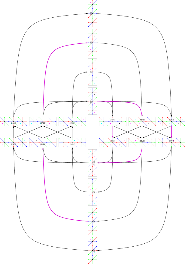
Figure 9.2: Diagram of the “circular lattice” obtained from Figure 9.1 by allowing the special face to be flipped (magenta edges).

Part IV Proofs of existence in the toroidal case

Chapter 10 Different proofs for triangulations

In the plane, the proof of existence of Schnyder wood is usually done quite easily by using a so-called shelling order (or canonical order, see [37]). This method consists is starting from the outer face and removing the vertices one by one. It leads to a simple linear time algorithm to compute a Schnyder wood. We do not see how to generalize the shelling order method for the torus since the objects that are then considered are too regular/homogeneous and there is no special face (and thus no particular starting point) playing the role of outer face.

We present in this chapter several proof of existence for toroidal triangulation with some consequences. Theses proofs also help to understand interesting structural properties of 3-orientations of toroidal maps. We propose to start with triangulations which are simpler and the proofs are somewhat more intuitive. The case of general toroidal maps (in fact essentially 3-connected toroidal maps) is studied in next chapter.

10.1 Contracting vertices

In this section we prove existence of balanced Schnyder wood for triangulations by contracting edges until we obtain a triangulation with just one vertex. The toroidal triangulation on one vertex is represented on Figure 4.1 with a balanced Schnyder wood. Then the graph can be decontracted step by step to obtain a balanced Schnyder wood of the original triangulation.

Given a toroidal triangulation $G$, the contraction of a non-loop-edge $e$ of $G$ is the operation consisting of continuously contracting $e$ until merging its two ends. We note $G/e$ the obtained map. On Figure 10.1 the contraction of an edge $e$ is represented. Note that only one edge of each multiple edges that is created is preserved (edge $e_{wx}$ and $e_{wy}$ on the figure).

$G$		$G/e$

Figure 10.1: The contraction operation for triangulations

Note that the contraction operation is also defined when some vertices are identified (see Figure 10.2): $x=u$ and $y=v$ (the case represented on the figure), or $x=v$ and $y=u$ (corresponding to the symmetric case with a diagonal in the other direction).

$G$		$G/e$

Figure 10.2: The contraction operation when some vertices are identified.

The contraction operation enables to prove the following:

Theorem 10

A toroidal triangulation admits a balanced Schnyder wood.

Proof.  Suppose the theorem is false and let $G$ be a toroidal triangulation, with no contractible loop nor homotopic multiple edges, that does not admit a balanced Schnyder wood and that has the minimum number of vertices. The graph $G$ is not a single vertex, otherwise it is easy to find a balanced Schnyder wood of it (see Figure 4.1). Then one can find an edge $e$ in $G$ such that its contraction preserves the fact that $G$ is a toroidal triangulation with no contractible loop nor homotopic multiple edges (see [42]). Let $G^{\prime}=G/e$ be the toroidal map obtained after contracting $e$.

By minimality, the graph $G^{\prime}$ has a balanced Schnyder wood. Note that since $G^{\prime}$ is a toroidal triangulation, all edges are oriented in one direction only. We now prove how to extend the Schnyder wood of $G^{\prime}$ to a Schnyder wood of $G$. Let $u,v$ be the two extremities of $e$ and $x,y$ the two vertices of $G$ such that the two faces incident to $e$ are $A=u,v,x$ and $B=v,u,y$ in clockwise order (see Figure 10.1). Note that $u$ and $v$ are distinct by definition of edge contraction but that $x$ and $y$ are not necessarily distinct, nor distinct from $u$ and $v$. Let $w$ be the vertex of $G^{\prime}$ resulting from the contraction of $e$. Let $e_{wx},e_{wy}$ be the two edges of $G^{\prime}$ represented on Figure 10.1 (these edges are identified and form a loop on Figure 10.2).

There are different cases corresponding to the different possibilities of orientation and coloring of the edges $e_{wx}$ and $e_{wy}$ in $G^{\prime}$. There should be $6$ cases depending on if $e_{wx}$ and $e_{wy}$ are both entering $w$, both leaving $w$ or one entering $w$ and one leaving $w$ (3 cases), multiplied by the coloring, both of the same color or not (2 cases). The case where $w$ has two edges leaving in the same color is not possible by the Schnyder property. So only $5$ cases remain represented on the left side of Figure 10.3. In the particular case where some vertices are identified (see Figure 10.2), there is a loop edge in $G^{\prime}$ that is uniquely colored, as on the left of Figure 10.4.

1
2
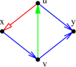
3
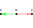
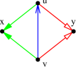
4
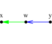
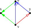
5
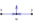
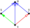
		$G^{\prime}$		$G$

Figure 10.3: Decontraction rules for triangulations.

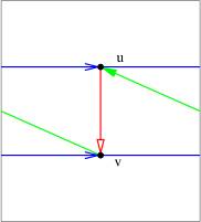
$G^{\prime}$		$G$

Figure 10.4: The decontraction operation when some vertices are identified.

In each case there might be several possibilities to orient and color the edges of $G$ incident to the faces $A$ and $B$ in order to obtain a Schnyder wood of $G$ from the Schnyder wood of $G^{\prime}$ (all the edges not incident to $A$ or $B$ are not modified). These different possibilities can easily be found by considering the angle labeling of $G$ and $G^{\prime}$ around vertices $u,v,w$.

For example, for case 1, the labeling of the angles in $G^{\prime}$ are depicted on the left of Figure 10.5. Since outside the contracted region, the edges are not modified, these labels have to be maintained during the decontraction process as shown on the middle of Figure 10.5. In this case, there are exactly three possible orientations and colorings of the edges of $G$ satisfying this labeling, one of these possibilities is represented on right part of Figure 10.5.

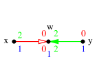
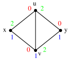
$G^{\prime}$	$G$	$G$

Figure 10.5: Angle labeling during decontraction for case 1 and the corresponding possible orientation and coloring of $G$.

For all the cases, there is always at least one possibility of orientation and coloring of $G$ satisfying the Schnyder property and one such possibility is represented on the right side of Figures 10.3 and 10.4. Since we are considering edges that are oriented in one direction only, there is no face whose boundary is a monochromatic cycle by the Schnyder property. So after decontraction we still have a Schnyder wood. Moreover one can check that the value $\gamma$ of any non-contractible cycle is not modified during the decontraction process. For this one can consider all the possible ways that a cycle may go through the contracted region and then check that the value of $\gamma$ is the same in $G$ and $G^{\prime}$. Thus the resulting Schnyder wood is balanced. $\Box$

Note that Theorem 10 confirms that Conjecture 1 is true when $g=1$. The proof is quite simple and can be turned into a linear time algorithm to find an balanced Schnyder wood. The main difficulty lies in finding sequence of edges that can be contracted in linear time.

An edge $e$ is said to be contractible if it is not a loop and if after contracting $e$ and identifying the borders of the two newly created length two faces, one obtains a triangulation that is still without contractible loop or homotopic multiple edges.

Consider an edge $e$ of $G$ with distinct ends $u,v$, and with incident faces $uvx$ and $vuy$, such that these vertices appear in clockwise order around the corresponding face (so we are in the situation of Figure 10.1). The edge $e$ is contractible if and only if, every walk enclosing an open disk containing a face other than $uvx$ and $vuy$, goes through an edge distinct from $e$ at least three times. Equivalently $e$ is non-contractible if and only if it belongs to a separating triangle or $u,v$ are both incident to a loop-edge $\ell_{u},\ell_{v}$, respectively, such that the walk of length four $(\ell_{u},e,\ell_{v},e)$ encloses an open disk with at least three faces (i.e. with at least one face distinct from $uvx$ and $vuy$). To avoid the latter case, if vertex $u$ is incident to a loop-edge $\ell_{u}$, we consider $e$ to be an edge that is consecutive to that loop, so that we have $x=u$. In such a case, if there is a loop $\ell_{v}$ incident to $v$ and a walk of length four of the form $(\ell_{u},e,\ell_{v},e)$ enclosing a disk with at least three faces, then there is also a separating triangle containing $e$. In the following we show how to find such separating triangle, if there is one. If $u$ and $v$ have more common neighbors, than simply $x$ and $y$, consider their second common neighbor going clockwise around $u$ from $e$ (the first one being $x$, and the last being $y$) and call it $x^{\prime}$. Call $y^{\prime}$ their second common neighbor going counterclockwise around $u$ from $e$. Now, either $uvx^{\prime}$ or $uvy^{\prime}$ is a separating triangle or the edge $e$ is contractible. We consider these two cases below:

• If $e$ is contractible, then it is contracted and we apply the procedure recursively to obtain a Schnyder wood of the contracted graph. Then we update the balanced Schnyder wood with the rules of Figures 10.3 and 10.4. Note that this update is done in constant time.

• If $uvx^{\prime}$ (resp. $uvy^{\prime}$) is a separating triangle, one can remove its interior, recursively obtain a toroidal Schnyder wood of the remaining toroidal triangulation, build a planar Schnyder wood of the planar triangulation inside $uvx^{\prime}$ (resp. $uvy^{\prime}$), and then superimpose the two (by eventually permuting the colors) to obtain a Schnyder wood of the whole graph. Note that computing a planar Schnyder wood can be done in linear time using a canonical ordering (see [37]).

The difficulty here is to test whether $uvx^{\prime}$ or $uvy^{\prime}$ are triangles. For that purpose, one first needs to compute a basis $(B_{1},B_{2})$ for the homology. Consider a spanning tree of the dual map $G^{*}$. The map obtained from $G$ by removing those edges is unicellular, and removing its treelike parts one obtains two cycles $(B_{1},B_{2})$ (intersecting on a path with at least one vertex) that form a basis for the homology. This can be computed in linear time for $G$ and then updated when some edge is contracted or when the interior of some separating triangle is removed. The updating takes constant time when some edge is contracted, and it takes $O(n^{\prime})$ time when removing $n^{\prime}$ vertices in the interior of some separating triangle. The overall cost of constructing and maintaining the basis is thus linear in the size of $G$. Then a closed walk of length three $W$, given with an arbitrary orientation, encloses a region homeomorphic to an open disk if and only if $W$ crosses $B_{i}$ from right to left as many times as $W$ crosses $B_{i}$ from left to right, for every $i\in\{1,2\}$. This test can be done in constant time for $uvx^{\prime}$ and $uvy^{\prime}$ once the half edges on the right and left sides of the cycles $B_{i}$ are marked. Marking the half edges of $G$ and maintaining this marking while contracting edges or while removing the interior of separating triangles can clearly be done in linear time. We thus have that the total running time to compute a balanced Schnyder wood of $G$ is linear.

Note that from a balanced Schnyder wood, one can easily obtain in linear time the minimal balanced Schnyder wood w.r.t. a special face $f_{0}$ by applying the method discuss in Section 5.2. Thus the total running time to compute a minimal balanced Schnyder wood is linear.

The proof of Theorem 10 can easily be generalized to essentially 3-connected toroidal maps. This is done in Chapter 11 in which we moreover do some tedious extra efforts to obtain the existence of crossing Schnyder woods and not only balanced Schnyder woods. Unfortunately Chapter 11 does not lead to a linear algorithm.

We do not see how to generalize the proof of Theorem 10 to higher genus surfaces. Indeed it is not always possible to find rules to decontract a vertex that has outdegree more than three. In the example of Figure 10.6 where the two considered edges incident to $w$ are outgoing, there is no way to orient and color the decontracted graph in order to maintain a Schnyder wood by keeping he orientation and coloring of edges that are not represented on the right part of the figure.

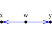
Figure 10.6: How to decontract a vertex of outdegree strictly more than $3$?

10.2 Reversing oriented subgraphs

In this section we obtain a proof of existence of crossing Schnyder woods by understanding some structural property on the set of $3$-orientations of a toroidal triangulation. In Section 10.2.1, we flip non-contractible cycles to move between the different lattices of homologous $3$-orientations in order to go from any lattice into the balanced lattice. Indeed we transform any $3$-orientation into a half-crossing Schnyder wood with this method. In Section 10.2.2, we flip 0-homologous oriented subgraphs to move inside the balanced lattice from a half-crossing Schnyder wood to a crossing Schnyder wood. The combination of the two sections gives a linear time algorithm to find a crossing Schnyder wood for a toroidal triangulation.

10.2.1 Non-contractible cycles

We first show several properties of 3-orientations of toroidal triangulations. By Theorem 2, a simple toroidal triangulation admits a 3-orientation. This can be shown to be true also for non-simple triangulations, for example using edge-contraction as explained in Section 10.1.

Consider a toroidal triangulation $G$ and a 3-orientation of $G$. Let $G^{\infty}$ be the universal cover of $G$.

Lemma 40

A cycle $C$ of $G^{\infty}$ of length $k$ has exactly $k-3$ edges leaving $C$ and directed toward the interior of $C$.

Proof.  Let $x$ be the number of edges leaving $C$ and directed toward the interior of $C$. Consider the cycle $C$ and its interior as a planar graph $C^{o}$. Euler’s formula gives $n^{\prime}-m^{\prime}+f^{\prime}=2$ where $n^{\prime},m^{\prime},f^{\prime}$ are respectively the number of vertices, edges and faces of $C^{o}$. Every inner vertex has exactly outdegree $3$, so $m^{\prime}=3(n^{\prime}-k)+k+x$. Every inner face has size three so $2m^{\prime}=3(f^{\prime}-1)+k$. Considering these equalities, one obtain that $x=k-3$ as claimed. $\Box$

As in Chapter 1, for an edge $e$ of $G$, we define the middle walk from $e$ as the sequence of edges $(e_{i})_{i\geq 0}$ obtained by the following method. Let $e_{0}=e$. If the edge $e_{i}$ is entering a vertex $v$, then the edge $e_{i+1}$ is chosen in the three edges leaving $v$ as the edge in the “middle” coming from $e_{i}$. The difference from Chapter 1 is that now a middle walk never ends since there is no outer vertex.

A directed cycle $M$ of $G$ is said to be a middle cycle if every vertex $v$ of $M$ has exactly one edge leaving $v$ on the left of $M$ (and thus exactly one edge leaving $v$ on the right of $M$). Note that a middle cycle $C$ satisfies $\gamma(C)=0$. Note that if $M$ is a middle cycle, and $e$ is an edge of $M$, then the middle walk from $e$ consists of the sequence of edges of $M$ repeated periodically. Note that a middle cycle is non-contractible, otherwise in $G^{\infty}$ it forms a contradiction to Lemma 40. Similar arguments lead to:

Lemma 41

Two middle cycles that are weakly homologous are either vertex-disjoint or equal.

We have the following useful lemma concerning middle walks and middle cycles:

Lemma 42

A middle walk always ends on a middle cycle.

Proof.  Start from any edge $e_{0}$ of $G$ and consider the middle walk $W=(e_{i})_{i\geq 0}$ from $e_{0}$. The graph $G$ has a finite number of edges, so some edges will be used several times in $W$. Consider a minimal subsequence $e_{k},\ldots,e_{\ell}$ such that no edge appears twice and $e_{k}=e_{\ell+1}$. Thus $W$ ends periodically on the sequence of edges $e_{k},\ldots,e_{\ell}$. We prove that $e_{k},\ldots,e_{\ell}$ is a middle cycle.

Assume that $k=0$ for simplicity. Thus $e_{0},\ldots,e_{\ell}$ is an Eulerian subgraph $E$. If $E$ is a cycle then it is a middle cycle and we are done. So we can consider that it visits some vertices several times. Let $e_{i},e_{j}$, with $0\leq i<j\leq\ell$, such that $e_{i},e_{j}$ are both leaving the same vertex $v$. By definition of $\ell$, we have $e_{i}\neq e_{j}$. Let $A$ and $B$ be the two closed walks $e_{i},\ldots,e_{j-1}$ and $e_{j},\ldots,e_{i-1}$, respectively, where indices are modulo $\ell+1$.

Consider a copy $v_{0}$ of $v$ in the universal cover $G^{\infty}$. Define the walk $P$ obtained by starting from $v_{0}$ following the edges of $G^{\infty}$ corresponding to the edges of $A$, and then to the edges of $B$. Similarly, define the walk $Q$ obtained by starting from $v_{0}$ following the edges of $B$, and then the edges of $A$. The two walks $P$ and $Q$ both start from $v_{0}$ and both end at the same vertex $v_{1}$ that is a copy of $v$. Note that $v_{1}$ and $v_{0}$ may coincide. All the vertices that are visited on the interior of $P$ and $Q$ have exactly one edge leaving on the left and exactly one edge leaving on the right. The two walks $P$ and $Q$ may intersect before they end at $v_{1}$ thus we define $P^{\prime}$ and $Q^{\prime}$ as the subwalks of $P$ and $Q$ starting from $v_{0}$, ending on the same vertex $u$ (possibly distinct from $v_{1}$ or not) and such that $P^{\prime}$ and $Q^{\prime}$ are not intersecting on their interior vertices. Then the union of $P^{\prime}$ and $Q^{\prime}$ forms a cycle $C$ of $G^{\infty}$. All the vertices of $C$ except possibly $v_{0}$ and $u$, have exactly one edge leaving $C$ and directed toward the interior of $C$, a contradiction to Lemma 40. $\Box$

A consequence of Lemma 42 is that any 3-orientation of a toroidal triangulation has a middle cycle. The 3-orientation of the toroidal triangulation on the left of Figure 4.1 is an example where there is a unique middle cycle (the diagonal).

By Lemma 42, a middle walk $W$ always ends on a middle cycle. Let us denote by $M_{W}$ this middle cycle and $P_{W}$ the part of $W$ before $M_{W}$. Note that $P_{W}$ may be empty. We say that a walk is leaving a cycle $C$ if its starting edge is incident to $C$ and leaving $C$.

Let us now prove the main lemma of this section.

Lemma 43

$G$ admits a 3-orientation with two middle cycles that are not weakly homologous.

Proof.  Suppose by contradiction that there is no 3-orientation of $G$ with two middle cycles that are not weakly homologous. We first prove the following claim:

Claim 4

There exists a 3-orientation of $G$ with a middle cycle $M$, a middle walk $W$ leaving $M$ and $M_{W}=M$.

Proof.  Suppose by contradiction that there is no 3-orientation of $G$ with a middle cycle $M$, a middle walk $W$ leaving $M$ and $M_{W}=M$. We first prove the following:

(1) Any 3-orientation of $G$, middle cycle $M$ and middle walk $W$ leaving $M$ are such that $M$ does not intersect the interior of $W$.

Assume by contradiction that $M$ intersects the interior of $W$. By assumption, cycles $M_{W}$ and $M$ are weakly homologous and $M_{W}\neq M$. Thus by Lemma 41, they are vertex-disjoint. So $M$ intersects the interior of $P_{W}$. Assume by symmetry that $P_{W}$ is leaving $M$ on its left side. If $P_{W}$ is entering $M$ from its left side, in $G^{\infty}$, the edges of $P_{W}$ plus $M$ form a cycle contradicting Lemma 40. So $P_{W}$ is entering $M$ from its right side. Hence $M_{W}$ intersects the interior of $P_{W}$ on a vertex $v$. Let $e$ be the edge of $P_{W}$ leaving $v$. Then the middle cycle $M_{W}$ and the middle walk $W^{\prime}$ starting from $e$ satisfies $M_{W^{\prime}}=M_{W}$, contradicting the hypothesis. So $M$ does not intersect the interior of $W$. This proves (1).

Consider a 3-orientation, a middle cycle $M$ and a middle walk $W$ leaving $M$ such that the length of $P_{W}$ is maximized. By assumption $M_{W}$ is weakly homologous to $M$ and $M_{W}\neq M$. Assume by symmetry that $P_{W}$ is leaving $M$ on its left side. (10.2.1) implies that $M$ does not intersect the interior of $W$. Let $v$ (resp. $e_{0}$) be the starting vertex (resp. edge) of $W$. Consider now the 3-orientation obtained by reversing $M_{W}$. Consider the middle walk $W^{\prime}$ starting from $e_{0}$. Walk $W^{\prime}$ follows $P_{W}$, then arrives on $M_{W}$ and crosses it (since $M_{W}$ has been reversed). (10.2.1) implies that $M$ does not intersect the interior of $W^{\prime}$. Similarly, (10.2.1) applied to $M_{W}$ and $W^{\prime}\setminus P_{W}$ (the walk obtained from $W^{\prime}$ by removing the first edges corresponding to $P_{W}$), implies that $M_{W}$ does not intersect the interior of $W^{\prime}\setminus P_{W}$. Thus, $M_{W^{\prime}}$ is weakly homologous to $M_{W}$ and $M_{W^{\prime}}$ is in the interior of the region between $M$ and $M_{W}$ on the right of $M$. Thus $P_{W^{\prime}}$ strictly contains $P_{W}$ and is thus longer, a contradiction. $\Diamond$

By Claim 4, consider a 3-orientation of $G$ with a middle cycle $M$ and a middle walk $W$ leaving $M$ such that $M_{W}=M$. Note that $W$ is leaving $M$ from one side and entering it from the other side, otherwise $W$ and $M$ will contradicts Lemma 40. Let $e_{0}$ be the starting edge of $W$. Let $v,u$ be the starting and ending point of $P_{W}$, respectively, where $u=v$ may occur. Consider the 3-orientation obtained by reversing $M$. Let $Q$ be the directed path from $u$ to $v$ along $M$ ($Q$ is empty if $u=v$). Let $C$ be the directed cycle $P_{W}\cup Q$. We compute the value $\gamma$ of $C$. If $u\neq v$, then $C$ is almost everywhere a middle cycle, except at $u$ and $v$. At $u$, it has two edges leaving on its right side, and at $v$ it has two edges leaving on its left side. So we have $\gamma(C)=0$. If $u=v$, then $C$ is a middle cycle and $\gamma(C)=0$. Thus, in any case $\gamma(C)=0$. Note that furthermore $\gamma(M)=0$ holds. The two cycles $M,C$ are non-contractible and not weakly homologous, so any non-contractible cycle of $G$ has $\gamma$ equal to zero by Lemma 34.

Consider the middle walk $W^{\prime}$ from $e_{0}$. By assumption $M_{W^{\prime}}$ is weakly homologous to $M$. The beginning $P_{W^{\prime}}$ is the same as for $P_{W}$. As we have reversed the edges of $M$, when arriving on $u$, path $P_{W^{\prime}}$ crosses $M$ and continues until reaching $M_{W^{\prime}}$. Thus $M_{W^{\prime}}$ intersects the interior of $P_{W^{\prime}}$ at a vertex $v^{\prime}$. Let $u^{\prime}$ be the ending point of $P_{W^{\prime}}$ (note that we may have $u^{\prime}=v^{\prime}$). Let $P^{\prime}$ be the non-empty subpath of $P_{W^{\prime}}$ from $v^{\prime}$ to $u^{\prime}$. Let $Q^{\prime}$ be the directed path from $u^{\prime}$ to $v^{\prime}$ along $M_{W^{\prime}}$ ($Q^{\prime}$ is empty if $u^{\prime}=v^{\prime}$). Let $C^{\prime}$ be the non-contractible directed cycle $P^{\prime}\cup Q^{\prime}$. We compute $\gamma(C^{\prime})$. The cycle $C^{\prime}$ is almost everywhere a middle cycle, except at $v^{\prime}$. At $v^{\prime}$, it has two edges leaving on its left or right side, depending on $M_{W^{\prime}}$ crossing $P_{W^{\prime}}$ from its left or right side. Thus, we have $\gamma(C^{\prime})=\pm 2$, a contradiction. $\Box$

By Lemma 43, for any toroidal triangulation, there exists a 3-orientation with two middle cycles that are not weakly homologous. By Lemma 34, this implies that any non-contractible cycle of $G$ has value $\gamma$ equal to zero so the $3$-orientation corresponds to a balanced Schnyder wood.

Note that $\gamma(C)=0$ for any non-contractible cycle $C$ does not necessarily imply the existence of two middle cycle that are not weakly homologous. The 3-orientation of the toroidal triangulation of Figure 8.8 is an example where $\gamma(C)=0$ for any non-contractible cycle $C$ but all the middle cycle are weakly homologous.

By combining Lemma 43 and Theorem 4, we obtain the following:

Theorem 11

A toroidal triangulation admits a half-crossing Schnyder wood.

Proof.  By Lemma 43, there exists a 3-orientation with two middle cycles that are not weakly homologous. By Lemma 34, any non-contractible cycle of $G$ has value $\gamma$ equal to zero. Thus the 3-orientation corresponds to a balanced Schnyder wood. In a Schnyder wood, a middle cycle corresponds to a monochromatic cycle. Since there are two middle cycles that are not weakly homologous, there are two crossing monochromatic cycles and the Schnyder wood is half-crossing. $\Box$

The proof presented in this section helps to understand the structure of $3$-orientations in toroidal triangulations. Indeed, it shows how to transform any $3$-orientation into a half-crossing Schnyder wood by reversing non-contractible cycles. It can be transformed into a linear algorithm to find an half-crossing Schnyder wood in a toroidal triangulation. First one has to find a $3$-orientation and this can be done in linear time by contracting edges as explained in Section 10.1. Then one start a middle walk from any edge. This walk ends on a middle cycle $C$. One picks any edge that is leaving $C$ and start a new middle walk from this edge. Each time the walk ends on a middle cycle $C^{\prime}$ that is weakly homologous to $C$, cycle $C^{\prime}$ is reversed and thus the middle walk can continue further until it crosses $C$. Then the obtained orientation corresponds to a crossing Schnyder wood.

For a triangulation on a genus $g\geq 2$ orientable surface we already know that there exists an orientation of the edges such that every vertex has outdegree at least $3$, and divisible by $3$ by Theorem 3. Can one apply the same method as here, i.e. reverse middle cycles, to obtain a Schnyder wood? First, one has to find the good notion of “middle” when dealing with special vertices of degree $6,9,...$ We believe that one should consider that “middle” is obtained by choosing any edge that is leaving $1\bmod 3$ edges on the left (and thus $1\bmod 3$ edges on the right). Note that their might be several choices depending on the outdegree of the vertex. Such a definition follows the notion of monochromatic paths that we want to achieve (see Figure 3.1). Then, unfortunately, the conclusion of Lemma 42 is false. Already when $g=2$, there might exist “middle” walks whose ending part is not a cycle. Figure 10.7 gives an example of an orientation of the edges of the triangulation of Figure 3.9 where every vertex has outdegree at least $3$, and divisible by $3$. The two vertices that are circled have outdegree 6. A “middle” periodic walk is depicted in green, it is not a cycle and forms an “eight”. On this example one can try to reverse the edges of the eight or of subcycles of middle walks in order to obtain a Schnyder wood but this method is not working on this example even if the process is repeated. Thus something more has to be found.

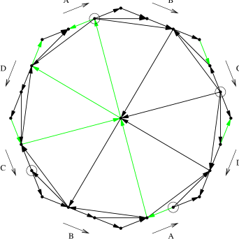
Figure 10.7: Orientation of a triangulation of the double torus where a “middle” walk form an eight.

Theorem 11 has some consequences concerning realizers. A nonempty family $\mathcal{R}$ of linear orders on the vertex set $V$ of a simple graph $G$ is called a realizer of $G$ if for every edge $e$, and every vertex $x$ not in $e$, there is some order $<_{i}\in\mathcal{R}$ so that $y<_{i}x$ for every $y\in e$. The dimension [25] of $G$, is defined as the least positive integer $t$ for which $G$ has a realizer of cardinality $t$. Realizers are usually used on finite graphs, but here we allow $G$ to be an infinite simple graph.

Schnyder woods where originally defined by Schnyder [50] to prove that a finite planar map $G$ has dimension at most $3$. A consequence of Theorem 11 is an analogous result for the universal cover of a toroidal map:

Theorem 12

The universal cover of a toroidal map has dimension at most three.

Proof.  Let $G$ be a toroidal map. By eventually adding edges to $G$ we may assume that $G$ is a toroidal triangulation. By Theorem 11, it admits a half-crossing Schnyder wood. For $i\in\{0,1,2\}$, let $<_{i}$ be the order induced by the inclusion of the regions $R_{i}$ in $G^{\infty}$ (see Section 3.6). That is $u<_{i}v$ if and only if $R_{i}(u)\subsetneq R_{i}(v)$. Let $<^{\prime}_{i}$ be any linear extension of $<_{i}$ and consider $\mathcal{R}=\{<^{\prime}_{0},<^{\prime}_{1},<^{\prime}_{2}\}$. Let $e$ be any edge of $G^{\infty}$ and $v$ be any vertex of $G^{\infty}$ not in $e$. Edge $e$ is in a region $R_{i}(v)$ for some $i$, thus $R_{i}(u)\subseteq R_{i}(v)$ for every $u\in e$ by Lemma 32.(i). As there is no edges oriented in two directions in a Schnyder wood of a toroidal triangulation, we have $R_{i}(u)\neq R_{i}(v)$ and so $u<_{i}v$. Thus $\mathcal{R}$ is a realizer of $G^{\infty}$. $\Box$

10.2.2 $0$-homologous oriented subgraphs

In this section we transform a half-crossing Schnyder wood of a toroidal triangulation into a crossing Schnyder wood by flipping $0$-homologous oriented subgraphs and thus obtain the following theorem:

Theorem 13

A toroidal triangulation admits a crossing Schnyder wood.

Proof.  Consider a toroidal triangulation $G$ and suppose by contradiction that $G$ does not admit a crossing Schnyder wood. By Theorem 11, $G$ admits a half-crossing Schnyder wood. Consider the set $\mathcal{H}$ of half-crossing Schnyder woods of $G$ with a coloring such that they are $i$-crossing all for the same color $i$. By assumption, Schnyder woods of $\mathcal{H}$ are not crossing, thus, by Theorem 9, all the $(i-1)$-cycles and the $(i+1)$-cycles are reversely homologous. Consider the subset $\mathcal{H}^{\prime}$ of $\mathcal{H}$ that minimizes the winding number (defined in Section 6.2). Let $\omega$ be the winding number of elements of $\mathcal{H}^{\prime}$ (so $\omega_{i}=0$ and $\omega_{i-1}=\omega_{i+1}=\omega$). Among all the element of $\mathcal{H}^{\prime}$, consider $H$ the half-crossing Schnyder wood that minimizes the number of $(i+1)$-cycles.

Consider a vertex $v$ that is in the intersection of a $i$-cycle $C$ and a $(i+1)$-cycle $C^{\prime}$. Then we are in one of the three cases depicted on the left side of Figure 10.8 (the color blue plays the role of color $i$ in the figures). If the winding number of $H$ is $1$, then we are in first case. If the winding number is strictly more than $1$, then $C^{\prime}$ is going either “down” (second case), or “up” (third case) according to $C$ being “vertical”.

Consider the path $P_{i-1}(v)$ obtained by following edges of color $i-1$ from $v$. Except on it starting point $v$, the path $P_{i}(v)$ cannot intersect $C^{\prime}$, otherwise it contradicts the fact that there exists a $(i-1)$-cycle reversely homologous to $C^{\prime}$. Consider the subpath $P$ of $P_{i}(v)$ starting from $v$ and ending on the $\omega^{th}$ intersection with $C$. Path $P$, cycle $C^{\prime}$ and a part of $C$ define a region $R$ (depicted in gray on Figure 10.8) whose border forms a $0$-homologous oriented subgraph $T$ oriented counterclockwise according to $R$. Consider the Schnyder wood $H^{\prime}$ obtained by reversing all the edges of $T$. The different cases are represented on the right side of Figure 10.8. The colors of the edges on $T$ get $+1$. The colors of the edges in the interior of $R$ get $-1$. The colors of the edges that are not in $R$ are not modified.

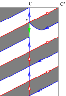
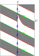
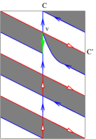
H	H’

Figure 10.8: Left: original Schnyder wood, right: Schnyder wood obtained after reversing the edges on the border of the gray region.

Note that in each case of Figure 10.8, there is a $i$-cycle intersecting the $(i-1)$-cycle corresponding to the reversal of $C^{\prime}$. Thus the obtained Schnyder wood is half-crossing. It is not crossing by assumption. Moreover its winding number is $1$. Thus, by the choice of $H$, the winding number of $H$ is also $1$ and we are in fact in the first case of Figure 10.8.

Schnyder wood $H^{\prime}$ is either $i$-crossing or $(i-1)$-crossing. Suppose by contradiction that it is $(i-1)$-crossing. By Theorem 9, the $i$- and $(i+1)$-cycles are reversely homologous. Note that there is a $i$-cycle crossing $C$ from right to left. Thus the $(i+1)$-cycles should cross $C$ from left to right. But this is impossible by the Schnyder property since $C$ is made of edges of color $i$ going “up” and edges of color $i+1$ going “down”. So the obtained Schnyder wood is $i$-crossing and all the $(i-1)$-cycles and $(i+1)$-cycles are reversely homologous.

We claim that a $(i+1)$-cycle cannot enter inside the region $R$. It cannot enter inside $R$ by crossing $C^{\prime}$ since $C^{\prime}$ is now a $(i-1)$-cycle and it should be reversely homologous to it. It cannot enter by the rest of the border of $R$ by the Schnyder property. So finally there is no $(i+1)$-cycle intersecting $R$. Recall that edges that are not in $R$ are not modified from $H$ to $H^{\prime}$, so $H^{\prime}$ has strictly less $(i+1)$-cycles than $H$ and winding number $1$, contradicting the choice of $H$. $\Box$

The proof of Theorem 13 can be turned into a linear time algorithm to find a crossing Schnyder wood in a toroidal triangulation. First one has to apply the method of Section 10.2.1 to obtain a half-crossing Schnyder wood in linear time. One should test if the obtained Schnyder wood is crossing. This can be done in linear time by following three monochromatic path from a vertex and check if their ending periodic monochromatic cycles intersect or not. If the half-crossing Schnyder wood has winding number strictly greater than $1$, then one apply the transformation described on Figure 10.8 once to get a half-crossing Schnyder wood with winding number $1$. One should check that the obtained Schnyder wood is crossing or not. If it is crossing we are done. Suppose it is not crossing but $i$-crossing. Then one should consider the set $\mathcal{C}$ of all the $(i+1)$-cycles, and apply the transformations described on Figure 10.8 by picking one by one a cycle in $C$. After each step the elements of $\mathcal{C}$ that are no more $(i+1)$-cycles in the current Schnyder wood are removed from $\mathcal{C}$. When $C$ is empty we have a crossing Schnyder wood. All the considered transformations are done one disjoint part of the triangulation and thus in total this can be done in linear time.

We do not know if this method can be generalized to essentially-3-connected toroidal maps. In Section 10.2.1 we are considering middle walks and here monochromatic paths to defined some oriented cycles that have to be flipped. For essentially 3-connected toroidal maps maps, we have to work in the primal-dual-completion where some more complex object have to be considered since oriented cycles have to be defined on primal-, dual- and edge-vertices. Then it is not only a “middle” or “monochromatic” property that should be considered and most of the intuition is lost.

Nevertheless in Chapter 11, we add additional requirement to the contraction method presented in Section 10.1 to prove existence of crossing Schnyder woods for essentially-3-connected toroidal maps. One drawback of Chapter 11 is that it does not lead to a linear algorithm. So if one really wants to keep linear complexity, then the above method is the best that we are able to do in linear time and one might be interesting into generalizing it to essentially 3-connected toroidal maps.

The existence of crossing Schnyder woods for toroidal triangulations implies the following theorem.

Theorem 14

A toroidal triangulation contains three non-contractible and not weakly homologous cycles that are pairwise edge-disjoint.

Proof.  One just has to apply Theorem 13 to obtain a crossing Schnyder wood and then, for each color $i$, choose an arbitrarily $i$-cycle. These cycles are edge-disjoint as there is no bioriented edges for triangulations. Moreover they are not homologous by Lemma 28. $\Box$

Note that, in the case of simple toroidal triangulations, there exists a stronger form of Theorem 14 (see Theorem 15 in next section) .

10.3 Gluing two planar Schnyder woods

In this section we present a proof of existence of Schnyder woods that consists in cutting a simple toroidal triangulation into two planar near-triangulations (i.e. whose inner faces have size three), find planar Schnyder woods of these maps and glue them on their boundaries to obtain a toroidal Schnyder wood of the original triangulation.

Fijavz [28] proved a useful result concerning existence of particular non homologous cycles in toroidal triangulations with no loop and no multiple edges. (Recall that in this manuscript we are less restrictive as we allow non-contractible loops and multiple edges that are not homotopic.)

Theorem 15 ([28])

A simple toroidal triangulation contains three non-contractible and not weakly homologous cycles that all intersect on one vertex and that are pairwise disjoint otherwise.

Note that Theorem 15 is not true for all toroidal triangulations as shown by the example on Figure 10.9, whereas the weak version, Theorem 14, is true for all triangulations.

Figure 10.9: A toroidal triangulation that does not contain three non-contractible and not weakly homologous cycles that all intersect on one vertex and that are pairwise disjoint otherwise.

We use Theorem 15 to cut a simple triangulation and past planar Schnyder woods in the two created regions. First, we need the following lemma:

Lemma 44

If $G$ is a connected planar near-triangulation whose outer face is a cycle, and with three vertices $x_{0},x_{1},x_{2}$ on its outer face such that the three outer paths between the $x_{i}$ are chordless, then $G^{\prime}$ is internally 3-connected for vertices $x_{i}$.

Proof.  Let $G^{\prime}$ be the graph obtained from $G$ by adding a vertex $z$ adjacent to the three vertices $x_{i}$. We have to prove that $G^{\prime}$ is 3-connected. Let $S$ be a separator of $G^{\prime}$ of minimum size and suppose by contradiction that $1\leq|S|\leq 2$. Let $G^{\prime\prime}=G^{\prime}\setminus S$.

For $v\in S$, the vertices of $N_{G^{\prime}}(v)\setminus S$ should appear in several connected components of $G^{\prime\prime}$, otherwise $S\setminus\{v\}$ is also a separator of $G^{\prime}$. Since $G$ is a planar near-triangulation, the neighbors of an inner vertex $v$ of $G$ form a cycle, thus there are at least two vertex-disjoint paths between any two vertices of $N(v)$ in $G^{\prime}\setminus\{v\}$. So $S$ contains no inner vertex of $G$. Similarly, the three neighbors of $z$ in $G^{\prime}$ belong to a cycle of $G^{\prime}\setminus\{z\}$ (the outer face of $G$), so $S$ does not face $z$. So $S$ contains only vertices that are on the outer face of $G$.

Let $v\in S$. Vertex $v$ is on the outer face of $G$ so its neighbors in $G$ form a path $P$ where the two extremities of $P$ are the two neighbors of $v$ on the outer face of $G$. Again if $v$ is one of the $x_{i}$, then its neighbors in $G^{\prime}$ belong to a cycle containing $z,x_{i-1},x_{i+1}$, so $v$ is not one of the $x_{i}$. So $S$ contains an inner vertex $u$ of $P$. Vertex $u$ is also on the outer face of $G$ so $uv$ is a chord of the outer cycle of $G$. As the three outer paths between the $x_{i}$ are chordless, we have that $u,v$ lie on two different outer paths between pairs of $x_{i}$. But then all the vertices of $P\setminus\{u\}$ are in the same components of $G^{\prime\prime}$ because of $z$, a contradiction. $\Box$

Now we prove the existence of some particular crossing Schnyder woods for simple toroidal triangulations.

Theorem 16

A simple toroidal triangulation admits a crossing Schnyder wood with three monochromatic cycles of different colors all intersecting on one vertex and that are pairwise disjoint otherwise.

Proof.  Let $G$ be a simple toroidal triangulation. By Theorem 15, let $C_{0},C_{1},C_{2}$ be three non-contractible and not weakly homologous cycles of $G$ that all intersect on one vertex $x$ and that are pairwise disjoint otherwise. By eventually shortening the cycles $C_{i}$, we can assume that the three cycles $C_{i}$ are chordless. By symmetry, we can assume that the six edges $e_{i},e^{\prime}_{i}$ of the cycles $C_{i}$ incident to $x$ appear around $x$ in the counterclockwise order $e_{0},e^{\prime}_{2},e_{1},e^{\prime}_{0},e_{2},e^{\prime}_{1}$ (see Figure 10.10). The cycles $C_{i}$ divide $G$ into two regions, denoted $R_{1},R_{2}$ such that $R_{1}$ is the region situated in the counterclockwise sector between $e_{0}$ and $e^{\prime}_{2}$ of $x$ and $R_{2}$ is the region situated in the counterclockwise sector between $e^{\prime}_{2}$ and $e_{1}$ of $x$. Let $G_{i}$ be the subgraph of $G$ contained in the region $R_{i}$ (including the three cycles $C_{i}$).

Figure 10.10: Notations of the proof of Theorem 16.

Let $G^{\prime}_{1}$ (resp. $G^{\prime}_{2}$) be the graph obtained from $G_{1}$ (resp. $G_{2}$) by replacing $x$ by three vertices $x_{0},x_{1},x_{2}$, such that $x_{i}$ is incident to the edges in the counterclockwise sector between $e_{i+1}$ and $e^{\prime}_{i}$ (resp. $e^{\prime}_{i}$ and $e_{i-1}$) (see Figure 10.11). The two graphs $G^{\prime}_{1}$ and $G^{\prime}_{2}$ are planar near-triangulations and the $C_{i}$ are chordless, so by Lemma 44, they are internally 3-connected planar maps for vertices $x_{i}$. The vertices $x_{0},x_{1},x_{2}$ appear in counterclockwise order on the outer face of $G^{\prime}_{1}$ and $G^{\prime}_{2}$. By Theorem 1, the two graphs $G^{\prime}_{i}$ admit planar Schnyder woods rooted at $x_{0},x_{1},x_{2}$. Orient and color the edges of $G$ that intersect the interior of $R_{i}$ by giving them the same orientation and coloring as in a planar Schnyder wood of $G^{\prime}_{i}$. Orient and color the cycle $C_{i}$ in color $i$ such that it is entering $x$ by edge $e^{\prime}_{i}$ and leaving $x$ by edge $e_{i}$. We claim that the orientation and coloring that is obtained is a Schnyder wood of $G$ (see Figure 10.11).

\begin{picture}(9302.0,9302.0)(3300.0,-8462.0)\end{picture}

Figure 10.11: Gluing two planar Schnyder woods into a toroidal one to prove Theorem 16.

Clearly, any interior vertex of the region $R_{i}$ satisfies the Schnyder property. Let us show that it is also satisfied for any vertex $v$ of a cycle $C_{i}$ distinct from $x$. In a Schnyder wood of $G^{\prime}_{1}$, the cycle $C_{i}$ is oriented in two direction, from $x_{i-1}$ to $x_{i}$ in color $i$ and from $x_{i}$ to $x_{i-1}$ in color $i-1$. Thus the edge leaving $v$ in color $i+1$ is an inner edge of $G^{\prime}_{1}$ and vertex $v$ has no edges entering in color $i+1$. Symmetrically, in $G^{\prime}_{2}$ the edge leaving $v$ in color $i-1$ is an inner edge of $G^{\prime}_{2}$ and vertex $v$ has no edges entering in color $i-1$. Then one can paste $G^{\prime}_{1}$ and $G^{\prime}_{2}$ along $C_{i}$, orient $C_{i}$ in color $i$ and see that $v$ satisfies the Schnyder property. The definition of $G^{\prime}_{i}$, and the orientation of the cycles is done so that $x$ satisfies also the Schnyder property. The cycles $C_{i}$ form three monochromatic cycles of different colors that are all intersecting on one vertex and that are pairwise disjoint otherwise and thus the Schnyder wood is crossing. $\Box$

The proof of Theorem 16 can be transformed into a polynomial algorithm but we do not know its exact complexity. The (non published) proof of Theorem 15 is itself based on a result of Robertson and Seymour [47] on disjoint paths.

We do not see how to adapt the method presented here if the map is non simple, not a triangulation, or in higher genus. For non simple triangulation, Theorem 15 is false as shown by Figure 10.9. For essentially 3-connected toroidal map, even if one find a way to cut the map, we do not know how to deal with vertices on the border of the resulting planar maps since they might have degree $2$ and then the planar map is not internally 3-connected. In higher genus we have no idea of what could be a generalization of Theorem 15.

A Schnyder wood is point-crossing if it is crossing and there are three monochromatic cycles of different colors all intersecting in one vertex (not necessarily disjoint otherwise). Theorem 16 shows the existence of Schnyder woods that are point-crossing and that have winding number $1$ for simple triangulation. Thus it is particularly interesting since it is the only proof of such result that we know. Winding number $1$ and crossing property is not always possible for non-simple toroidal triangulations (see for example the graph of Figure 10.9) but on the contrary the existence of point-crossing Schnyder woods might be generalizable to all triangulations?

Note that in the Schnyder wood obtained by Theorem 16, we do not know if there are several monochromatic cycles of one color or not. We wonder whether Theorem 16 can be modified as follow: Does a simple toroidal triangulation admits a Schnyder wood such that each color induces a connected subgraph (so there is just one monochromatic cycle per color)? Can one additionally require that it is point-crossing and/or has winding number $1$?

Chapter 11 Existence for essentially 3-connected toroidal maps

In this chapter we generalize the proof of Section 10.1 to essentially 3-connected toroidal maps, moreover we show that at each decontraction step the crossing property can be preserved. Thus we obtain the existence of crossing Schnyder woods for almost all essentially 3-connected toroidal maps, except a very particular family of toroidal maps for which only intersecting Schnyder woods exists.

11.1 Contraction of essentially 3-connected toroidal maps

Given a map $G$ embedded on a surface. The angle map [48] of $G$ is a map $A(G)$ on this surface whose vertices are the vertices of $G$ plus the vertices of $G^{*}$ (i.e. the faces of $G$), and whose edges are the angles of $G$, each angle being incident with the corresponding vertex and face of $G$. Note that if $G$ has no contractible loop nor homotopic multiple edges, then every face of $G$ has degree at least $3$ in $A(G)$.

Mohar and Rosenstiehl [43] proved that a map $G$ is essentially 2-connected if and only if the angle map $A$ of $G$ has no pair of (multiple) edges bounding a disk (as every face in an angle map is a quadrangle, such disk would contain some vertices of $G$). The following lemma naturally extends this characterization to essentially 3-connected toroidal maps.

Lemma 45

A toroidal map $G$ is essentially 3-connected if and only if the angle map $A(G)$ has no walk of length at most four bounding a disk which is not a face.

Proof.  ($\Longrightarrow$) Any walk in $A(G)$ of length at most 4 bounding a disk which is not a face lifts to a cycle of length at most 4 bounding a disk which is not a face in $A(G^{\infty})$. Thus such a walk implies the existence of a small separator in $G^{\infty}$, contradicting its 3-connectedness.

($\Longleftarrow$) According to [43], if $G$ is essentially 2-connected, $A(G)$ has no walk of length 2 bounding a disk. If $G$ is essentially 2-connected but not essentially 3-connected, then $A(G^{\infty})$ has a cycle $C$ of length 4 bounding a disk which is not a face. Let $W$ be the walk of $A(G)$ corresponding to $C$. Walk $W$ contains a subwalk bounding a disk. Since $A(G)$ is bipartite, this subwalk has even length. Since $A(G)$ is essentially 2-connected, it has no such walk of length 2. Thus $W$ bounds a disk. Finally, this disk is not a single face since otherwise $C$ would bound a single face in $A(G^{\infty})$. $\Box$

Given a toroidal map $G$, the contraction of a non-loop-edge $e$ of $G$ is the operation consisting of continuously contracting $e$ until merging its two ends. We note $G/e$ the obtained map. On Figure 11.1 the contraction of an edge $e$ is represented. We consider three different cases corresponding to whether the faces adjacent to $e$ have size three or not. Note that only one edge of each set of multiple edges that is created is preserved. The contraction operation is also define when $t=u$ and $y=v$ (the case represented on Figure 11.2), or $x=v$ and $z=u$ (corresponding to the symmetric case with a diagonal in the other direction).

$G$		$G/e$
(a)		(a’)
(b)		(b’)
(c)		(c’)

Figure 11.1: The contraction operation

(d)		(d’)
(e)		(e’)
(f)		(f’)

Figure 11.2: The contraction operation when some vertices are identified.

A non-loop edge $e$ of an essentially 3-connected toroidal map is contractible if the contraction of $e$ keeps the map essentially 3-connected. We have the following lemma:

Lemma 46

An essentially 3-connected toroidal map that is not reduced to a single vertex has a contractible edge.

Proof.  Let $G$ be an essentially 3-connected toroidal map with at least 2 vertices. Note that for any non-loop edge $e$, the map $A(G/e)$ has no walk of length $2$ bounding a disk which is not a face, otherwise, $A(G)$ contains a walk of length at most $4$ bounding a disk which is not a face and thus, by Lemma 45, $G$ is not essentially 3-connected.

Suppose by contradiction that contracting any non-loop edge $e$ of $G$ yields a non essentially 3-connected map $G/e$. By Lemma 45, the angle map $A(G)$ has no walk of length at most four bounding a disk which is not a face. For any non-loop edge $e$, let $W_{4}(e)$ be a 4-walk of $A(G/e)$ bounding a disk, which is maximal in terms of the faces it contains. Among all the non-loop edges, let $e$ be the one such that the number of faces in $W_{4}(e)$ is minimum. Let $W_{4}(e)=(v_{1},f_{1},v_{2},f_{2})$ and assume that the endpoints of $e$, say $a$ and $b$, are contracted into $v_{2}$ (see Figure 11.3). Note that by maximality of $W_{4}(e)$, $v_{1}$ and $v_{2}$ do not have any common neighbor $f$ out of $W_{4}(e)$, such that $(v_{1},f,v_{2},f_{1})$ bounds a disk.

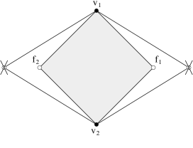
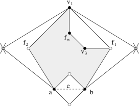
$G/e$		$G$

Figure 11.3: Notations of the proof of Lemma 46

Assume one of $f_{1}$ or $f_{2}$ has a neighbor inside $W_{4}(e)$. By symmetry, assume $v_{3}$ is a vertex inside $W_{4}(e)$ such that there is a face $F=(v_{1},f_{1},v_{3},f_{w})$ in $A(G/e)$, with eventually $f_{w}=f_{2}$. Consider now the contraction of the edge $v_{1}v_{3}$. Let $P(v_{1},v_{3})=(v_{1},f_{x},v_{y},f_{z},v_{3})$ be the path from $v_{1}$ to $v_{3}$ corresponding to $W_{4}(v_{1}v_{3})$ and $P(a,b)=(a,f_{2},v_{1},f_{1},b)$ the path corresponding to $W_{4}(e)$. Suppose that all the faces of $W_{4}(v_{1}v_{3})$ are in $W_{4}(e)$, then with $F$, $W_{4}(e)$ contains more faces than $W_{4}(v_{1}v_{3})$, a contradiction to the choice of $e$. So in $A(G)$, path $P(v_{1},v_{3})$ crosses $P(a,b)$.

If $v_{y}=a$ or $v_{y}=b$. Then $v_{1},v_{y},f_{z},v_{3}$ are in $W_{4}(e)$, so $f_{x}$ is out and $(v_{1},f_{x},v_{2},f_{1})$ bounds a disk, a contradiction. So $v_{y}\neq a$ and $v_{y}\neq b$ and thus $f_{z}=f_{1}$ or $f_{z}=f_{2}$. If $f_{z}=f_{1}$, then the cycle $(v_{1},f_{x},v_{y},f_{1})$ bounds a face by Lemma 45. This implies that $W_{4}(v_{1}v_{3})$ bounds a face, a contradiction. So $f_{z}\neq f_{1}$ and thus $f_{z}=f_{2}$. If $f_{w}=f_{2}$, then similarly, the cycle $(v_{1},f_{x},v_{y},f_{2})$ bounds a face by Lemma 45. This implies that $W_{4}(v_{1}v_{3})$ bounds a face, a contradiction. So $f_{w}\neq f_{2}$. Then $(v_{1},f_{2},v_{3},f_{w})$ bounds a face by Lemma 45 and then $f_{w}$ has degree $2$ in $A(G)$, a contradiction.

Assume now that none of $f_{1}$ or $f_{2}$ has a neighbor inside $W_{4}(e)$. Let $f^{\prime}_{1}$, $f^{\prime}_{2}$, $f_{3}$ and $f^{\prime}_{3}$ be vertices of $A(G)$ such that $(v_{1},f_{1},b,f^{\prime}_{1})$, $(v_{1},f_{2},a,f^{\prime}_{2})$ and $(a,f_{3},b,f^{\prime}_{3})$ are faces (see Figure 11.4). Suppose $f^{\prime}_{1}=f^{\prime}_{2}=f^{\prime}_{3}$. Then in $A(G/e)$, the face $f^{\prime}_{1}$ is deleted (among the 2 homologous multiple edges between $v_{1},v_{2}$ that are created, only one is kept in $G/e$). Then $W_{4}(e)$ bounds a face, a contradiction. Thus there exists some $i$ such that $f^{\prime}_{i}\neq f^{\prime}_{i+1}$. Assume that $i=1$ (resp. $i=2$ or 3), and let $v_{3}$ and $f^{\prime\prime}$ be such that there is a face $(v_{1},f^{\prime}_{1},v_{3},f^{\prime\prime})$ in $A(G)$ (resp. $(a,f^{\prime}_{2},v_{3},f^{\prime\prime})$ or $(b,f^{\prime}_{3},v_{3},f^{\prime\prime})$). As above considering the contraction of the edge $v_{1}v_{3}$ (resp. $av_{3}$ or $bv_{3}$) yields a contradiction.

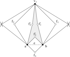
Figure 11.4: Notations of the proof of Lemma 46

$\Box$

Lemma 46 shows that an essentially 3-connected toroidal map can be contracted step by step by keeping it essentially 3-connected until obtaining a map with just one vertex. The two essentially 3-connected toroidal maps on one vertex are represented on Figure 11.5 with a Schnyder wood. The map of Figure 11.5.(a), the 3-loops, admits a crossing Schnyder wood, and the map of Figure 11.5.(b), the 2-loops, admits an intersecting Schnyder wood.

(a) The 3-loops		(b) The 2-loops

Figure 11.5: The two essentially 3-connected toroidal maps on one vertex.

It would be convenient if one could contract any essentially 3-connected toroidal map until obtaining one of the two maps of Figure 11.5 and then decontract the map to obtain an intersecting Schnyder wood of the original map. Unfortunately, we are not able to prove that the intersecting property can be preserved during the decontraction process.

On the example of Figure 11.6, it is not possible to decontract the graph $G^{\prime}$ (Figure 11.6.(a)), and extend its intersecting Schnyder wood to $G$ (Figure 11.6.(b)) without modifying the edges that are not incident to the contracted edge $e$. Indeed, if we keep the edges non incident to $e$ unchanged, there are only two possible ways to extend the coloring in order to preserve the Schnyder property, but none of them leads to an intersecting Schnyder wood.

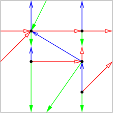
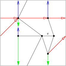
(a)		(b)

Figure 11.6: (a) The map obtained by contracting the edge $e$ of the map (b). It is not possible to color and orient the black edges of (b) to obtain an intersecting Schnyder wood.

Fortunately most essentially 3-connected toroidal maps admits crossing Schnyder woods and not only intersecting Schnyder woods and we are able to preserve the crossing property during the decontraction process (see Section 11.2).

A toroidal map is basic if it consists of a non-contractible cycle on $n$ vertices, $n\geq 1$, plus $n$ homologous loops (see Figure 7.4).

Lemma 47

A basic toroidal map admits an intersecting Schnyder wood but no crossing Schnyder wood.

Proof.  Basic toroidal maps admits intersecting Schnyder woods as shown by Figure 7.4. Suppose that a basic toroidal map $G$ on $n$ vertices admits a crossing Schnyder wood. Consider one of the vertical loop $e$ and suppose by symmetry that it is oriented upward in color $1$. In a crossing Schnyder wood, all the monochromatic cycles of different colors are not weakly homologous, thus all the loops homologous to $e$ are also oriented upward in color $1$ and they are not bioriented. It remains just a cycle on $n$ vertices for edges of color $0$ and $2$. Thus the Schnyder wood is the one of Figure 7.4 and not crossing, a contradiction. $\Box$

To prove existence of crossing Schnyder woods for general essentially 3-connected toroidal maps, instead of contracting these maps to one of the two maps of Figure 11.5, we contract them to the map of Figure 11.5.(a), the 3-loops, or to the map of Figure 11.7, the brick, that both admits crossing Schnyder woods. (One can draw the universal cover of the brick to understand its name.)

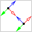
Figure 11.7: The brick, an essentially 3-connected toroidal map with two vertices, given with a crossing Schnyder wood.

Now we can state our main existence result:

Theorem 17

A toroidal map admits a crossing Schnyder wood if and only if it is an essentially 3-connected non-basic toroidal map. Moreover, basic toroidal maps admits intersecting Schnyder woods.

Note that Theorem 17 confirms Conjecture 2 for $g=1$. The proof of this theorem is postponed to Section 11.3. The main difficulty is to show that one can decontract a crossing Schnyder wood by preserving the crossing property. This is done in next section by first relaxing the definition of crossing and then proving a decontraction lemma. Before we prove the following contraction lemma:

Lemma 48

A non-basic essentially 3-connected toroidal map can be contracted to the 3-loops (Figure 11.5.(a)) or to the brick (Figure 11.7) by keeping the toroidal map essentially 3-connected.

Proof.  Let us prove the lemma by induction on the number of edges of the map. As the 3-loop and the brick are the only non-basic essentially 3-connected toroidal maps with at most 3 edges, the lemma holds for the maps with at most 3 edges. Consider now a non-basic essentially 3-connected toroidal map $G$ with at least $4$ edges. As $G$ has at least 2 vertices, it has at least one contractible edge by Lemma 46. If $G$ has a contractible edge $e$ which contraction yields a non-basic map $G^{\prime}$, then by induction hypothesis on $G^{\prime}$ we are done. Let us prove that such an edge always exists. We assume by contradiction, that the contraction of any contractible edge $e$ yields a basic map $G^{\prime}$. Let us denote $v_{i}$, with $1\leq i\leq n$, the vertices of $G^{\prime}$ in such a way that $(v_{1},v_{2},\ldots,v_{n})$ is a cycle of $G^{\prime}$. We can assume that $v_{1}$ is the vertex resulting of the contraction of $e$. Let $u$ and $v$ be the endpoints of $e$ in $G$.

Suppose first that $u$ or $v$ is incident to a loop in $G$. By symmetry, we can assume that $v$ is incident to a loop and that $u$ is in the cylinder between the loops around $v$ and $v_{n}$ (if $n=1$ then $v_{n}=v$) and $u$ is the only vertex here. Since $G$ is non-basic and $u$ has at least 3 incident edges, two of them go to the same vertex but are not homotopic multiple edges. Since after the contraction of $e$ there is only one edge left in the cylinder, we can deduce that $u$ has at least two edges in common with $v$. On the other side since $G$ is essentially 3-connected $u$ has an edge $e^{\prime}$ with $v_{n}$. This edge $e^{\prime}$ is contractible since its contraction yields a map containing the basic graph on $n$ vertices. But since this map has two edges linking $(uv_{n})$ and $v$, it is non-basic. So $G$ has a contractible edge which contraction produces a non-basic map, contradicting our assumption.

Suppose now that $u$ and $v$ do not have incident loop, we thus have that $G$ contains a (non-contractible) cycle $C$ of length $2$ containing $e$. Let $e^{\prime}$ be the other edge of $C$. Since $G$ is essentially 3-connected, both $u$ and $v$ have at least degree 3, and at least one of them has an incident edge on the left (resp. right) of $C$. If $n=1$, since $G$ has at least 4 edges there are 2 edges, say $f_{1}$ and $f_{2}$ between $u$ and $v$ and distinct from $e$ and $e^{\prime}$ that are not homotopic multiple edges. The edges $f_{1}$ and $f_{2}$ remain distinct edges in $G^{\prime}$. So $G^{\prime}$ has one vertex and 3 edges, it is thus non-basic. Assume now that $n\geq 2$. In this case $u$ and $v$ are contained in a cylinder bordered by the loops at $v_{2}$ and at $v_{n}$ (with eventually $n=2$). We can assume that $u$ has at least one incident edge $f_{1}$ on the left of $C$ to $v_{n}$, and that $v$ has at least one incident edge $f_{2}$ on the right of $C$ to $v_{2}$. In this case one can contract $f_{1}$ and note that the obtained map which contain at least 3 edges around $v$ ($e$, $e^{\prime}$ and $f_{2}$) is essentially 3-connected, and non-basic. So $G$ has a contractible edge which contraction produces a non-basic map, contradicting our assumption. $\Box$

11.2 Special decontraction preserving crossing

The goal of this section is to prove the following lemma:

Lemma 49

If $G$ is a toroidal map given with a non-loop edge $e$ whose extremities are of degree at least three and such that $G/e$ admits a crossing Schnyder wood, then $G$ admits a crossing Schnyder wood.

The proof of Lemma 49 is long and technical. There is a huge case analysis for the following reasons. One has to consider the different kind of contraction depicted on Figures 11.1 and 11.2. For each of these cases, one as to consider the different ways that the edges of $G/e$ that are labeled on the figures can be oriented and colored in a crossing Schnyder wood of $G/e$ see Figures 11.8 and 11.9. For each of these cases, one as to show that one can orient and color the edges of $G$ that are labeled on the figures to extend the crossing Schnyder wood of $G$ to a crossing Schnyder wood of $G/e$ (non-labeled edges keep the orientation and coloring they have in $G/e$). This would be quite easy if one just have to satisfy the Schnyder property like in Section 10.1, but satisfying the crossing property is much more complicated.

a.1			b.1			c.1
a.2			b.2			c.2
a.3			b.3			c.3
a.4			b.4			c.4
a.5			b.5			c.5
			b.6			c.6
			b.7			c.7
			b.8			c.8
			b.9			c.9
			b.10

Figure 11.8: Orientation and coloring possibilities for cases (a) (b) and (c).

Figure 11.9: Orientation and coloring for cases (d) (e) and (f).

We first need to relax the definition of crossing Schnyder wood:

Lemma 50

Let $G$ be a toroidal map given with an orientation and coloring of the edges of $G$ with the colors $0$, $1$, $2$, where every edge $e$ is oriented in one direction or in two opposite directions (each direction having a distinct color and being outgoing). The orientation and coloring is a crossing Schnyder wood if and only if it satisfies the following:

• Every vertex $v$ satisfies the Schnyder property.

• For each pair $i,j$ of different colors, there exists a $i$-cycle intersecting a $j$-cycle.

• There is no monochromatic cycles $C_{i},C_{j}$ of different colors $i,j$ such that $C_{i}=C_{j}^{-1}$.

Proof.  ($\Longrightarrow$) If we have a crossing Schnyder wood, then Property (T1) is clearly satisfied by definition. Property (T1) implies that there exists a monochromatic cycles of each color, thus Property (T2) is a consequence of the crossing property. Property (T3) is implied by Theorem 9.

($\Longleftarrow$) Conversely, suppose we have an orientation and coloring satisfying (T1), (T2), (T3). By (T3), there is no face the boundary is a monochromatic cycle since, by (T1), such a cycle would be colored one way in color $i$ and the other way in color $j$, and it contradicts (T3). Thus the orientation and coloring is a Schnyder wood.

Let us now prove that the Schnyder wood is crossing. Let $C_{i}$ be any $i$-cycle of color $i$. We have to prove that $C_{i}$ crosses at least one $(i-1)$-cycle and at least one $(i+1)$-cycle. Let $j$ be either $i-1$ or $i+1$. By (T2), there exists a $i$-cycle $C^{\prime}_{i}$ intersecting a $j$-cycle $C^{\prime}_{j}$ of color $j$. The two cycles $C^{\prime}_{i},C^{\prime}_{j}$ are not reversal by (T3), thus they are crossing. So the Schnyder wood is half-crossing and more precisely $i$-crossing or $j$-crossing and the two cycles $C_{i}$ and $C^{\prime}_{j}$ are crossing. $\Box$

Note that for toroidal triangulations, there is no edges oriented in two directions in an orientation and coloring of the edges satisfying (T1). So (T3) is automatically satisfied. Thus in the case of toroidal triangulations it is sufficient to have properties (T1) and (T2) to have a crossing Schnyder wood. This is not true in general as shown by the example of Figure 11.10 that satisfies (T1) and (T2) but that is not a crossing Schnyder wood. There is a monochromatic cycle of color $1$ (blue) that is not intersecting any monochromatic cycle of color $2$ (green).

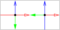
Figure 11.10: An orientation and coloring of the edges of a toroidal map satisfying (T1) and (T2) but that is not a crossing Schnyder wood.

By Lemma 50, instead of proving that the crossing property is preserved during the decontraction process, by considering intersections between every pair of monochromatic cycles, we prove (T2) and (T3). Property (T2) is simpler than the definition of crossing as it is considering just one intersection for each pair of colors instead of all the intersections. Even with this simplification proving (T2) is the main difficulty of the proof. For each considered cases, one has to analyze the different ways that the monochromatic cycles go through the contracted vertex or not and to show that there always exists a coloring and orientation of $G$ where (T2) is satisfied. In fact, among all the cases of Figures 11.8 and 11.9, we detail only one case completely to show how the proof goes. The numerous other cases can be proved similarly.

Proof of Lemma 49.

Let $u,v$ be the two extremities of $e$. Vertices $u$ and $v$ are of degree at least three. Depending on whether the faces incident to $e$ have size three or not, and that some vertices are identified or not, we are, by symmetry, in one of the cases (a), (b), (c), (d), (e), (f) of Figure 11.1 and 11.2. Let $G^{\prime}=G/e$ and consider a crossing Schnyder wood of $G^{\prime}$. Let $w$ be the vertex of $G^{\prime}$ resulting from the contraction of $e$.

Like in the proof of Theorem 10, for each case (a), (b), (c), (d), (e), (f), there are different cases to consider corresponding to the different possibilities of orientations and colorings of the labeled edges of $G^{\prime}$ in a crossing Schnyder wood of $G^{\prime}$. These cases are represented (up to symmetry) on Figure 11.8 for cases (a), (b), (c) and Figure 11.9 for cases (d), (e), (f). A dotted half-edge represent the possibility for an edge to be uni- or bidirected.

In each case, one can easily color and orient the edges of $G$ to satisfy (T1). Just the edges of $G$ that are labeled on Figures 11.1 and 11.2 have to be specified, all the other edges of $G$ keep the orientation and coloring that they have in the crossing Schnyder wood of $G^{\prime}$. There might be several possibilities to color and orient the edges in order to satisfy (T1). These different possibilities can easily be found by considering the angle labeling of $G$ and $G^{\prime}$ around vertices $u,v,w$ (as in the proof of Theorem 10).

For example, for case a.1, the labeling of the angles in $G^{\prime}$ are depicted on the left of Figure 10.5. There is exactly three possible orientations and colorings of the edges of $G$ satisfying this labeling and represented by cases a.1.1, a.1.2, a.1.3 on Figure 11.11.

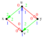
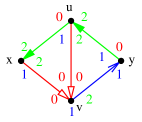
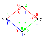
a.1.1		a.1.2		a.1.3

Figure 11.11: The three possible orientation and coloring of $G$ for case a.1.

One can check that for all cases of Figure 11.11, property (T3) is preserved. Indeed, if (T3) is not satisfied in $G$ after applying one of the possible orientation and coloring satisfying (T1), then there exists two monochromatic cycles $C,C^{\prime}$ of different colors that are reversal. By Lemma 50, there is no reversal cycles in the crossing Schnyder wood of $G^{\prime}$. Thus $C,C^{\prime}$ have to use a bidirected edge that is newly created. There is no such edges in the cases of Figure 11.11, so (T3) is always preserved in this case.

For the other cases (a), (b), (c), (d), (e), (f), it is just a little case analysis to identify among the orientation and coloring preserving (T1), which one also preserves (T3). We illustrate this for the case c.4. Figure 11.12 gives two possible orientation and coloring of $G$ preserving (T1) for case c.4. Only for the second case we are sure to preserve (T3). Indeed, in the first case the decontraction process might create a green cycle and a blue cycle that are reversal to each other. This is not possible in the second case as two reversal cycles will have to use the red-blue or green-blue edge. If the green-blue edge is used, then the two reversal cycles are green and blue, but the blue cycle continues with the red-blue edge, a contradiction. If the red-blue edge is used, then the two reversal cycles are red and blue and already present in $G^{\prime}$, a contradiction. We do not detail more this part that can easily be done for all cases.

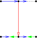
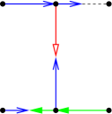
Figure 11.12: Discussion on (T3) preservation during decontraction of case c.4.

Among all the possible orientation and coloring of $G$ satisfying (T1) and (T3), we claim that there is always at least one that satisfies (T2) and thus gives a crossing Schnyder wood of $G$. Identifying which one satisfies (T2) depends on a huge case analysis concerning the behavior of the monochromatic cycles in $G^{\prime}$. and is the main difficulty of the proof. We illustrate this part by doing only case a.1 completely. This case is the most difficult cases for proving that (T2) can be preserved. We omit the proof of the numerous other cases that can be obtained with similar arguments.

The sector $[e_{1},e_{2}]$ of a vertex $w$, for $e_{1}$ and $e_{2}$ two edges incident to $w$, is the counterclockwise sector of $w$ between $e_{1}$ and $e_{2}$, including the edges $e_{1}$ and $e_{2}$. The sector $]e_{1},e_{2}]$, $[e_{1},e_{2}[$, and $]e_{1},e_{2}[$ are defined analogously by excluding the corresponding edges from the sectors.

We assume that we are in case a.1, where $e_{wx}=e_{0}(x)$ and $e_{wy}=e_{2}(y)$. We say that a monochromatic cycle $C$ of $G^{\prime}$ is safe if $C$ does not contain $w$. Depending on whether there are safe monochromatic cycles or not of each colors, it is a different argument that is used to prove that property (T2) can be preserved by one of the coloring of Figure 11.11. All the cases are considered below.

• There are safe monochromatic cycles of colors $\{0,1,2\}$.

Let $C^{\prime}_{0},C^{\prime}_{1},C^{\prime}_{2}$ be safe monochromatic cycles of color $0,1,2$ in $G^{\prime}$. As the Schnyder wood of $G^{\prime}$ is crossing, they pairwise intersects in $G^{\prime}$. Apply the coloring a.1.1 on $G$. As $C^{\prime}_{0},C^{\prime}_{1},C^{\prime}_{2}$ do not contain vertex $w$, they are not modified in $G$. Thus they still pairwise intersect in $G$. So (T2) is satisfied.

• There are safe monochromatic cycles of colors exactly $\{0,2\}$.

Let $C^{\prime}_{0},C^{\prime}_{2}$ be safe monochromatic cycles of color $0,2$ in $G^{\prime}$. Let $C^{\prime}_{1}$ be a $1$-cycle in $G^{\prime}$. As the Schnyder wood of $G^{\prime}$ is crossing, $C^{\prime}_{0},C^{\prime}_{1},C^{\prime}_{2}$ pairwise intersects in $G^{\prime}$. None of those intersections contain $w$ as $C^{\prime}_{0}$ and $C^{\prime}_{2}$ do not contain $w$. By (T1), the cycle $C^{\prime}_{1}$ enter $w$ in the sector $]e_{wx},e_{wy}[$ and leaves in the sector $]e_{wy},e_{wx}[$. Apply the coloring a.1.1 on $G$. The cycle $C^{\prime}_{1}$ is replaced by a new cycle $C_{1}=C^{\prime}_{1}\setminus\{w\}\cup\{u,v\}$. The cycles $C^{\prime}_{0},C^{\prime}_{1},C^{\prime}_{2}$ were intersecting outside $w$ in $G^{\prime}$ so $C^{\prime}_{0},C_{1},C^{\prime}_{2}$ are intersecting in $G$. So (T2) is satisfied.

• There are safe monochromatic cycles of colors exactly $\{1,2\}$.

Let $C^{\prime}_{1},C^{\prime}_{2}$ be safe monochromatic cycles of color $1,2$ in $G^{\prime}$. Let $C^{\prime}_{0}$ be a $0$-cycle in $G^{\prime}$. The cycles $C^{\prime}_{0},C^{\prime}_{1},C^{\prime}_{2}$ pairwise intersects outside $w$. The cycle $C^{\prime}_{0}$ enters $w$ in the sector $[e_{1}(w),e_{wx}[$, $[e_{wx},e_{wx}]$ or $]e_{wx},e_{2}(w)]$. Apply the coloring a.1.2 on $G$. Depending on which of the three sectors $C^{\prime}_{0}$ enters, it is is replaced by one of the three following cycle $C_{0}=C^{\prime}_{0}\setminus\{w\}\cup\{u,v\}$, $C_{0}=C^{\prime}_{0}\setminus\{w\}\cup\{x,v\}$, $C_{0}=C^{\prime}_{0}\setminus\{w\}\cup\{v\}$. In any of the three possibilities, $C_{0},C^{\prime}_{1},C^{\prime}_{2}$ are intersecting in $G$. So (T2) is satisfied.

• There are safe monochromatic cycles of colors exactly $\{0,1\}$.

This case is completely symmetric to the previous case where there are safe monochromatic cycles of colors exactly $\{1,2\}$.

• There are safe monochromatic cycles of color $2$ only.

Let $C^{\prime}_{2}$ be a safe $2$-cycle in $G^{\prime}$. Let $C^{\prime}_{0},C^{\prime}_{1}$ be monochromatic cycles of color $0,1$ in $G^{\prime}$.

Suppose that there exists a path $Q^{\prime}_{0}$ of color $0$, from $y$ to $w$ such that this path does not intersect $C^{\prime}_{2}$. Suppose also that there exists a path $Q^{\prime}_{1}$ of color $1$, from $y$ to $w$ such that this path does not intersect $C^{\prime}_{2}$. Let $C^{\prime\prime}_{0}=Q^{\prime}_{0}\cup\{e_{wy}\}$ and $C^{\prime\prime}_{1}=Q^{\prime}_{1}\cup\{e_{wy}\}$. By Lemma 6, cycles $C^{\prime\prime}_{0},C^{\prime\prime}_{1},C^{\prime}_{2}$ are non-contractible. Both of $C^{\prime\prime}_{0},C^{\prime\prime}_{1}$ do not intersect $C^{\prime}_{2}$ so by Lemma 26, they are both weakly homologous to $C^{\prime}_{2}$. Thus cycles $C^{\prime\prime}_{0},C^{\prime\prime}_{1}$ are weakly homologous to each other. The path $Q^{\prime}_{0}$ is leaving $C^{\prime\prime}_{1}$ at $y$ on the right side of $C^{\prime\prime}_{1}$. Since $C^{\prime\prime}_{1}$ and $C^{\prime\prime}_{0}$ are weakly homologous, the path $Q^{\prime}_{0}$ is entering $C^{\prime\prime}_{1}$ at least once from its right side. This is in contradiction with the Schnyder property. So we can assume that one of $Q^{\prime}_{0}$ or $Q^{\prime}_{1}$ as above does not exist.

Suppose that in $G^{\prime}$, there does not exist a path of color $0$, from $y$ to $w$ such that this path does not intersect $C^{\prime}_{2}$. Apply the coloring a.1.1 on $G$. Cycle $C^{\prime}_{1}$ is replaced by $C_{1}=C^{\prime}_{1}\setminus\{w\}\cup\{u,v\}$, and intersect $C^{\prime}_{2}$. Let $C_{0}$ be a $0$-cycle of $G$. Cycle $C_{0}$ has to contain $u$ or $v$ or both, otherwise it is a safe cycle of $G^{\prime}$ of color $0$. In any case it intersects $C_{1}$. If $C_{0}$ contains $v$, then $C^{\prime}_{0}=C_{0}\setminus\{v\}\cup\{w\}$ and so $C_{0}$ is intersecting $C^{\prime}_{2}$ and (T2) is satisfied. Suppose now that $C_{0}$ does not contain $v$. Then $C_{0}$ contains $u$ and $y$, the extremity of the edge leaving $u$ in color $0$. Let $Q_{0}$ be the part of $C_{0}$ consisting of the path from $y$ to $u$. The path $Q^{\prime}_{0}=Q_{0}\setminus\{u\}\cup\{w\}$ is from $y$ to $w$. Thus by assumption $Q^{\prime}_{0}$ intersects $C^{\prime}_{2}$. So $C_{0}$ intersects $C^{\prime}_{2}$ and (T2) is satisfied.

Suppose now that in $G^{\prime}$, there does not exist a path of color $1$, from $y$ to $w$ such that this path does not intersect $C^{\prime}_{2}$. Apply the coloring a.1.2 on $G$. Depending on which of the three sectors $C^{\prime}_{0}$ enters, $[e_{1}(w),e_{wx}[$, $[e_{wx},e_{wx}]$ or $]e_{wx},e_{2}(w)]$, it is is replaced by one of the three following cycle $C_{0}=C^{\prime}_{0}\setminus\{w\}\cup\{u,v\}$, $C_{0}=C^{\prime}_{0}\setminus\{w\}\cup\{x,v\}$, $C_{0}=C^{\prime}_{0}\setminus\{w\}\cup\{v\}$. In any of the three possibilities, $C_{0}$ contains $v$ and intersect $C^{\prime}_{2}$. Let $C_{1}$ be a $1$-cycle of $G$. Cycle $C_{1}$ has to contain $u$ or $v$ or both, otherwise it is a safe cycle of $G^{\prime}$ of color $1$. Vertex $u$ has no edge entering it in color $1$ so $C_{1}$ does not contain $u$ and thus it contains $v$ and intersects $C_{0}$. Then $C_{1}$ contains $y$, the extremity of the edge leaving $v$ in color $1$. Let $Q_{1}$ be the part of $C_{1}$ consisting of the path from $y$ to $v$. The path $Q^{\prime}_{1}=Q_{1}\setminus\{v\}\cup\{w\}$ is from $y$ to $w$. Thus by assumption $Q^{\prime}_{1}$ intersects $C^{\prime}_{2}$. So $C_{1}$ intersects $C^{\prime}_{2}$ and (T2) is satisfied.

• There are safe monochromatic cycles of color $0$ only.

This case is completely symmetric to the case $\{2\}$.

• There are safe monochromatic cycles of color $1$ only.

Let $C^{\prime}_{1}$ be a safe $1$-cycle in $G^{\prime}$. Let $C^{\prime}_{0}$ and $C^{\prime}_{2}$ be monochromatic cycles of color $0$ and $2$ in $G^{\prime}$.

Suppose $C^{\prime}_{0}$ is entering $w$ in the sector $]e_{wx},e_{2}(w)]$. Apply the coloring a.1.3 on $G$. The $0$-cycle $C^{\prime}_{0}$ is replaced by $C_{0}=C^{\prime}_{0}\setminus\{w\}\cup\{v\}$ and thus contains $v$ and still intersect $C^{\prime}_{1}$. Depending on which of the three sectors $C^{\prime}_{2}$ enters, $[e_{0}(w),e_{wy}[$, $[e_{wy},e_{wy}]$ or $]e_{wy},e_{1}(w)]$, it is replaced by one of the three following cycles $C_{2}=C^{\prime}_{2}\setminus\{w\}\cup\{v\}$, $C_{2}=C^{\prime}_{2}\setminus\{w\}\cup\{y,v\}$, $C_{2}=C^{\prime}_{2}\setminus\{w\}\cup\{u,v\}$. In any case, $C_{2}$ contains $v$ and still intersect $C^{\prime}_{1}$. Cycle $C_{0}$ and $C_{2}$ intersect on $v$. So (T2) is satisfied.

The case where $C^{\prime}_{2}$ is entering $w$ in the sector $[e_{0}(w),e_{wy}[$ is completely symmetric and we apply the coloring a.1.2 on $G$.

It remains to deal with the case where $C^{\prime}_{0}$ is entering $w$ in the sector $[e_{1}(w),e_{wx}]$ and $C^{\prime}_{2}$ is entering $w$ in the sector $[e_{wy},e_{1}(w)]$. Suppose that there exists a path $Q^{\prime}_{0}$ of color $0$, from $y$ to $w$, entering $w$ in the sector $[e_{1}(w),e_{wx}]$, such that this path does not intersect $C^{\prime}_{1}$. Suppose also that there exists a path $Q^{\prime}_{2}$ of color $2$, from $x$ to $w$, entering $w$ in the sector $[e_{wy},e_{1}(w)]$, such that this path does not intersect $C^{\prime}_{1}$. Let $C^{\prime\prime}_{0}=Q^{\prime}_{0}\cup\{e_{wy}\}$ and $C^{\prime\prime}_{2}=Q^{\prime}_{2}\cup\{e_{wx}\}$. By Lemma 6, cycles $C^{\prime\prime}_{0},C^{\prime}_{1},C^{\prime\prime}_{2}$ are non-contractible. Cycles $C^{\prime\prime}_{0},C^{\prime\prime}_{2}$ do not intersect $C^{\prime}_{1}$ so by Lemma 26, they are weakly homologous to $C^{\prime}_{1}$. Thus cycles $C^{\prime\prime}_{0},C^{\prime\prime}_{2}$ are weakly homologous to each other. By (T3), we have $C^{\prime\prime}_{0}\neq(C^{\prime\prime}_{2})^{-1}$. So cycle $C^{\prime\prime}_{2}$ is leaving $C^{\prime\prime}_{0}$. By (T1) and the assumption on the sectors, $C^{\prime\prime}_{2}$ is leaving $C^{\prime\prime}_{0}$ on its right side. Since $C^{\prime\prime}_{0}$ and $C^{\prime\prime}_{2}$ are weakly homologous, the path $Q^{\prime}_{2}$ is entering $C^{\prime\prime}_{0}$ at least once from its right side. This is in contradiction with the Schnyder property. So we can assume that one of $Q^{\prime}_{0}$ or $Q^{\prime}_{2}$ as above does not exist.

By symmetry, suppose that in $G^{\prime}$, there does not exist a path of color $0$, from $y$ to $w$, entering $w$ in the sector $[e_{1}(w),e_{wx}]$, such that this path does not intersect $C^{\prime}_{1}$. Apply the coloring a.1.3 on $G$. Depending on which of the two sectors $C^{\prime}_{2}$ enters, $[e_{wy},e_{wy}]$ or $]e_{wy},e_{1}(w)]$, it is is replaced by one of the two following cycle $C_{2}=C^{\prime}_{2}\setminus\{w\}\cup\{y,v\}$, $C_{2}=C^{\prime}_{2}\setminus\{w\}\cup\{u,v\}$. In any case, $C_{2}$ still intersects $C^{\prime}_{1}$. Let $C_{0}$ be a $0$-cycle of $G$. Cycle $C_{0}$ has to contain $u$ or $v$ or both, otherwise it is a safe cycle of $G^{\prime}$ of color $0$. Suppose $C_{0}$ does not contain $u$, then $C^{\prime}_{0}=C_{0}\setminus\{v\}\cup\{w\}$ and $C^{\prime}_{0}$ is not entering $w$ in the sector $[e_{1}(w),e_{wx}]$, a contradiction. So $C_{0}$ contains $u$. Thus $C_{0}$ contains $y$, the extremity of the edge leaving $u$ in color $0$, and it intersects $C_{2}$. Let $Q_{0}$ be the part of $C_{0}$ consisting of the path from $y$ to $u$. The path $Q^{\prime}_{0}=Q_{0}\setminus\{u\}\cup\{w\}$ is from $y$ to $w$ and entering $w$ in the sector $[e_{1}(w),e_{wx}]$. Thus by assumption $Q^{\prime}_{0}$ intersects $C^{\prime}_{1}$. So $C_{0}$ intersects $C^{\prime}_{1}$ and (T2) is satisfied.

• There are no safe monochromatic cycle.

Let $C^{\prime}_{0},C^{\prime}_{1},C^{\prime}_{2}$ be monochromatic cycles of color $0,1,2$ in $G^{\prime}$. They all pairwise intersect on $w$.

Suppose first that $C^{\prime}_{0}$ is entering $w$ in the sector $]e_{wx},e_{2}(w)]$. Apply the coloring a.1.3 on $G$. The $0$-cycle $C^{\prime}_{0}$ is replaced by $C_{0}=C^{\prime}_{0}\setminus\{w\}\cup\{v\}$ and thus contains $v$. Depending on which of the three sectors $C^{\prime}_{2}$ enters, $[e_{0}(w),e_{wy}[$, $[e_{wy},e_{wy}]$ or $]e_{wy},e_{1}(w)]$, it is is replaced by one of the three following cycle $C_{2}=C^{\prime}_{2}\setminus\{w\}\cup\{v\}$, $C_{2}=C^{\prime}_{2}\setminus\{w\}\cup\{y,v\}$, $C_{2}=C^{\prime}_{2}\setminus\{w\}\cup\{u,v\}$. In any case, $C_{2}$ contains $v$. Let $C_{1}$ be a $1$-cycle in $G$. Cycle $C_{1}$ has to contain $u$ or $v$ or both, otherwise it is a safe cycle of $G^{\prime}$ of color $1$. Vertex $u$ has no edge entering it in color $1$ so $C_{1}$ does not contain $u$ and thus it contains $v$. So $C_{0},C_{1},C_{2}$ all intersect on $v$ and (T2) is satisfied.

The case where $C^{\prime}_{2}$ is entering $w$ in the sector $[e_{0}(w),e_{wy}[$ is completely symmetric and we apply the coloring a.1.2 on $G$.

It remains to deal with the case where $C^{\prime}_{0}$ is entering $w$ in the sector $[e_{1}(w),e_{wx}]$ and $C^{\prime}_{2}$ is entering $w$ in the sector $[e_{wy},e_{1}(w)]$. Apply the coloring a.1.1 on $G$. Cycle $C^{\prime}_{1}$ is replaced by $C_{1}=C^{\prime}_{1}\setminus\{w\}\cup\{u,v\}$. Let $C_{0}$ be a $0$-cycle in $G$. Cycle $C_{0}$ has to contain $u$ or $v$ or both, otherwise it is a safe cycle of $G^{\prime}$ of color $0$. Suppose $C_{0}\cap\{v,x\}=\{v\}$, then $C_{0}\setminus\{v\}\cup\{w\}$ is a $0$-cycle of $G^{\prime}$ entering $w$ in the sector $]e_{wx},e_{2}(w)]$, contradicting the assumption on $C^{\prime}_{0}$. Suppose $C_{0}$ contains $u$, then $C_{0}$ contains $y$, the extremity of the edge leaving $u$ in color $0$. So $C_{0}$ contains $\{v,x\}$ or $\{u,y\}$. Similarly $C_{2}$ contains $\{v,y\}$ or $\{u,x\}$. In any case $C_{0},C_{1},C_{2}$ pairwise intersect. So (T2) is satisfied.

$\Box$

11.3 Proof of existence

We are now able to prove Theorem 17:

Proof of Theorem 17.

The second part of the theorem is clear by Lemma 47.

($\Longrightarrow$) If $G$ is a toroidal map given with a crossing Schnyder wood. Then, by Lemma 8, $G$ is essentially 3-connected and by Lemma 47, $G$ is not basic.

($\Longleftarrow$) Let $G$ be a non-basic essentially 3-connected toroidal map. By Lemma 48, $G$ can be contracted to the 3-loops or to the brick by keeping the map essentially 3-connected (so all the vertices have degree at least $3$). Both of these maps admit crossing Schnyder woods (see Figure 11.5.(a) and 11.7). So by Lemma 49 applied successively, $G$ admits a crossing Schnyder wood. $\square$

Here is a remark about how to compute a crossing Schnyder wood for an essentially 3-connected toroidal triangulation. Instead of completing the technical proof of Lemma 49 to know which coloring of the decontracted map has to be chosen among the possible choice to preserve the crossing property, one can proceed as follows. At each decontraction step, one can try all the possible decontraction that preserves the Schnyder property and check afterward which one gives a crossing Schnyder wood. This method gives a polynomial algorithm that is not linear since at each decontraction step there is already a test of the crossing property that takes linear time.

Part V Applications in the toroidal case

Chapter 12 Optimal encoding and bijection

12.1 Poulalhon and Schaeffer’s method

Poulalhon and Schaeffer introduced in [45] an elegant method (called here PS method for short) to linearly encode a planar triangulation $G$ with a binary word of length $\log_{2}\binom{4n}{n}\sim n\,\log_{2}(\frac{256}{27})\approx 3.2451\,n$ bits. This is asymptotically optimal since it matches the information theory lower bound. The method is the following. Consider the set of orientations of $G$ where inner vertices have outdegree $3$ and outer vertices have outdegree $1$. These set carries a structure of distributive lattice and one can consider its minimal element w.r.t. the outer face. Then, starting from the outer face, a special depth-first search algorithm is applied by “following” ingoing edges and “cutting” outgoing ones. The algorithm outputs a rooted spanning tree with exactly two leaves (also called stems) on each inner vertex from which the original triangulation can be recovered in a straightforward way. This tree can be encoded very efficiently. A nice aspect of this work, besides its interesting encoding properties, is that the method gives a bijection between planar triangulations and a particular type of plane trees with some consequences for counting and sampling planar triangulation.

Castelli Aleardi, Fusy and Lewiner [14] adapt PS method to encode planar triangulations with boundaries. A consequence is that a triangulation of any orientable surface can be encoded by cutting the surface along non-contractible cycles and see the surface as a planar map with boundaries. The obtained algorithm is asymptotically optimal (in terms of number of bits) but it is not linear, nor bijective.

We propose an alternative generalization of PS algorithm to higher genus whose execution on a minimal balanced toroidal Schnyder wood of a toroidal triangulation leads to a rooted unicellular map (which corresponds to the natural generalization of trees when going to higher genus). This map can be encoded optimally using $3.2451\,n$ bits. The algorithm can be performed in linear time and leads to a new bijection between toroidal triangulations and a particular type of unicellular maps.

The two main ingredients that make PS algorithm work in an orientation of a planar map are minimality and accessibility of the orientation. Minimality means that there is no clockwise cycle and can be translated with the terminology of section 5.2 by saying that it is minimal w.r.t. the outer face. Accessibility means that there exists a root vertex such that all the vertices have an oriented path directed toward the root vertex. Felsner’s result [23] concerning existence and uniqueness of a minimal $\alpha$-orientation as soon as an $\alpha$-orientation exists, enables several analogues of PS method to different kinds of planar maps, see [2, 6, 18]. In all these cases the accessibility of the considered $\alpha$-orientations is a consequence of the natural choice of $\alpha$, like in Poulalhon and Schaeffer’s original work [45] where any $3$-orientation of the inner edges of a planar triangulation is accessible for any choice of root vertex on the outer face. (Note that the conventions may differs in the literature: the role of outgoing and incoming edges are sometimes exchanged and/or the role of clockwise and counterclockwise.)

For higher genus, the minimality can be obtained by results of Section 5.2 showing that on any orientable surface the set of orientations of a given map having the same homology carries a structure of distributive lattice. But a given map on an orientable surface can have several $\alpha$-orientations (for the same given $\alpha$) that are not homologous (see for instance the example of Chapter 9). So the set of $\alpha$-orientations of a given map is now partitioned into distributive lattices contrarily to the planar case where there is only one lattice (and thus only one minimal element). For toroidal triangulations we manage to face this problem and maintain a bijection by using the balanced property of Chapter 8 that defines a canonical lattice.

The main issue while trying to extend PS algorithm to higher genus is the accessibility. Accessibility toward the outer face is given almost for free in the planar case because of Euler’s formula that sums to a strictly positive value. For an orientable surface of genus $g\geq 1$ new difficulties occur. Already in genus $1$ (the torus), even if the orientation is minimal and accessible PS algorithm can visit all the vertices but not all the angles of the map because of the existence of non-contractible cycles. Lemma 36 can be used to show that this problem never occurs for minimal balanced Schnyder woods. In genus $g\geq 2$ things get even more difficult with separating non-contractible cycles that make having accessibility of the vertices difficult to obtain.

Another problem is to recover the original map after the execution of the algorithm. If what remains after the execution of PS method is a spanning unicellular map then the map can be recovered with the same simple rules as in the plane. Unfortunately for many minimal orientations the algorithm leads to a spanning unicellular embedded graph that is not a map (the only face is not a disk) and it is not possible to directly recover the original map. Here again, the choice of the minimal balanced Schnyder wood ensures that this never happens.

12.2 General properties of Algorithm PS

We introduce the following reformulation of Poulalhon and Schaeffer’s original algorithm. This version is more general in order to be applicable to any orientation of any map on an orientable surface.

Algorithm PS

Input: An oriented map $G$ on an oriented surface $S$, a root vertex $v_{0}$ and a root edge $e_{0}$ incident to $v_{0}$.

Output: A graph $U$ with stems, embedded on the oriented surface $S$.

1. Let $v:=v_{0}$, $e:=e_{0}$, $U:=\emptyset$.

2. Let $v^{\prime}$ be the extremity of $e$ different from $v$.

   • $e$ is non-marked and entering $v$. Add $e$ to $U$ and let $v:=v^{\prime}$.

   • $e$ is non-marked and leaving $v$. Add a stem to $U$ incident to $v$ and corresponding to $e$.

   • $e$ is already marked and entering $v$. Do nothing.

   • $e$ is already marked and leaving $v$. Let $v:=v^{\prime}$.

3. Mark $e$.

4. Let $e$ be the next edge around $v$ in counterclockwise order after the current $e$.

5. While $(v,e)\neq(v_{0},e_{0})$ go back to 2.

6. Return $U$.

We show general properties of Algorithm PS in this section before considering toroidal triangulations in the forthcoming sections.

We insist on the fact that the output of Algorithm PS is a graph embedded on the same surface as the input map but that this embedded graph is not necessarily a map (i.e some faces may not be homeomorphic to open disks). In the following section we show that in our specific case the output $U$ is an unicellular map.

Consider any oriented map $G$ on an orientable surface given with a root vertex $v_{0}$ and a root edge $e_{0}$ incident to $v_{0}$. When Algorithm PS is considering a couple $(v,e)$ we see this like it is considering the angle at $v$ that is just before $e$ in counterclockwise order. The particular choice of $v_{0}$ and $e_{0}$ is thus in fact a particular choice of a root angle $a_{0}$ that automatically defines a root vertex $v_{0}$, a root edge $e_{0}$, as well as a root face $f_{0}$. From now on we consider that the input of Algorithm PS is an oriented map plus a root angle (without specifying the root vertex, face and edge).

The angle graph of $G$, is the graph defined on the angles of $G$ and where two angles are adjacent if and only if they are consecutive around a vertex or around a face. An execution of Algorithm PS can be seen as a walk in the angle graph. Figure 12.1 illustrates the behavior of the algorithm corresponding to Case 1 to 4. In each case, the algorithm is considering the angle in top left position and depending on the marking of the edge and its orientation the next angle that is considered is the one that is the end of the magenta arc of the angle graph. The cyan edge of Case 1 represents the edge that is added to $U$ by the algorithm. The stems of $U$ added in Case 2 are not represented in cyan, in fact we will represent them later by an edge in the dual. Indeed seeing the execution of Algorithm PS as a walk in the angle graph enables us to show that Algorithm PS behaves exactly the same in the primal or in the dual map (as explained later).

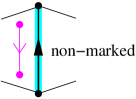
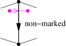
Case 1	Case 2
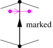
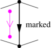
Case 3	Case 4

Figure 12.1: The four cases of Algorithm PS .

The crossing Schnyder wood of Figure 12.2 is the minimal balanced Schnyder wood of $K_{7}$ for the choice of $f_{0}$ corresponding to the shaded face. This example is used in all this chapter to illustrate Poulalhon and Schaeffer’s method.

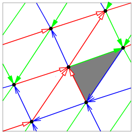
Figure 12.2: The minimal balanced Schnyder wood of $K_{7}$ w.r.t. the shaded face.

On Figure 12.3, we give an example of an execution of Algorithm PS on the orientation of Figure 12.2.

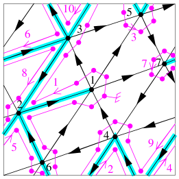
Execution	Output

Figure 12.3: An execution of Algorithm PS on $K_{7}$ given with the orientation corresponding to the minimal balanced Schnyder wood of Figure 12.2. Vertices are numbered in black. The root angle is identified by a root symbol and chosen in the face for which the orientation is minimal (i.e. the shaded face of Figure 12.2). The magenta arrows and numbers are here to help the reader to follow the cycle in the angle graph. The output $U$ is a toroidal unicellular map, represented here as an hexagon where the opposite sides are identified.

Let $a$ be a particular angle of the map $G$. It is adjacent to four other angles in the angle graph (see Figure 12.4). Let $v,f$ be such that $a$ is an angle of vertex $v$ and face $f$. The next-vertex (resp. previous-vertex) angle of $a$ is the angle appearing just after (resp. before) $a$ in counterclockwise order around $v$. Similarly, the next-face (resp. previous-face) angle of $a$ is the angle appearing just after (resp. before) $a$ in clockwise order around $f$. These definitions enable one to orient consistently the edges of the angle graph like in Figure 12.4 so that for every oriented edge $(a,a^{\prime})$, $a^{\prime}$ is a next-vertex or next-face angle of $a$.

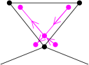
Figure 12.4: Orientation of the edges of the angle graph.

The different cases depicted in Figure 12.1 show that an execution of Algorithm PS is just an oriented walk in the angle graph (i.e. a walk that is following the orientation of the edges described in Figure 12.4). The condition in the while loop ensures that when the algorithm terminates, this walk is back to the root angle. The following proposition shows that the algorithm actually terminates:

Proposition 12

Consider an oriented map $G$ on an orientable surface and a root angle $a_{0}$. The execution of Algorithm PS on $(G,a_{0})$ terminates and corresponds to a cycle in the angle graph.

Proof.  We consider the oriented walk $W$ in the angle graph corresponding to the execution of Algorithm PS . Note that $W$ may be infinite. The walk $W$ starts with $a_{0}$, and if it is finite it ends with $a_{0}$ and contains no other occurrence of $a_{0}$ (otherwise the algorithm should have stopped earlier). Toward a contradiction, suppose that $W$ is not simple (i.e. some angles different from the root angle $a_{0}$ are repeated). Let $a\neq a_{0}$ be the first angle along $W$ that is met for the second time. Let $a_{1},a_{2}$ be the angles appearing before the first and second occurrence of $a$ in $W$, respectively. Note that $a_{1}\neq a_{2}$ by the choice of $a$.

If $a_{1}$ is the previous-vertex angle of $a$, then $a_{2}$ is the previous-face angle of $a$. When the algorithm considers $a_{1}$, none of $a$ and $a_{2}$ are already visited, thus the edge $e$ between $a$ and $a_{1}$ is not marked. Since the execution then goes to $a$ after $a_{1}$, we are in Case 2 and edge $e$ is oriented from $v$, where $v$ is the vertex incident to $a$. Afterward, when the algorithm reaches $a_{2}$, Case 3 applies and the algorithm cannot go to $a$, a contradiction. The case where $a_{1}$ is the previous-face angle of $a$ is similar.

So $W$ is simple. Since the angle graph is finite, $W$ is finite. So the algorithm terminates, thus $W$ ends on the root angle and $W$ is a cycle. $\Box$

In the next section we see that in some particular cases the cycle in the angle graph corresponding to the execution of PS algorithm (Proposition 12) can be shown to be Hamiltonian like on Figure 12.3.

By Proposition 12, an angle is considered at most once by Algorithm PS. This implies that the angles around an edge can be visited in different ways depicted on Figure 12.5. Consider an execution of Algorithm PS on $G$. Let $C$ be the cycle formed in the angle graph by Proposition 12. Let $P$ be the set of edges of the output $U$ (without the stems) and $Q$ be the set of dual edges of edges of $G$ corresponding to stems of $U$. These edges are represented on Figure 12.5 in cyan for $P$ and in yellow for $Q$. They are considered with the convention that the dual edge $e^{*}$ of an edge $e$ goes from the face on the left of $e$ to the face on the right of $e$. Note that $C$ does not cross an edge of $P$ or $Q$, and moreover $P$ and $Q$ do not intersect (i.e. an edge can be in $P$ or its dual in $Q$ but both cases cannot happen).

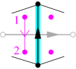
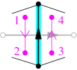
Case 1 alone	Case 1 and then 4
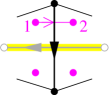
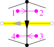
Case 2 alone	Case 2 and then 3

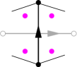
Not visited

Figure 12.5: The different cases of Algorithm PS seen in a dual way. The number of the angles gives the order in which the algorithm visits them (unvisited angles are not numbered). The edges of $P$ and $Q$ are respectively cyan and yellow.

One can remark that the cases of Figure 12.5 are dual of each other. One can see that Algorithm PS behaves exactly the same if applied on the primal map or on the dual map. The only modifications to make is to start the algorithm with the face $f_{0}$ as the root vertex, the dual of edge $e_{0}$ as the root edge and to replace counterclockwise by clockwise at Line 4. Then the cycle $C$ formed in the angle graph is exactly the same and the output is $Q$ with stems corresponding to $P$ (instead of $P$ with stems corresponding to $Q$). Note that this duality is also illustrated by the fact that the minimality of the orientation of $G$ w.r.t. the root face is nothing else than the accessibility of the dual orientation toward the root face. Indeed, a clockwise $0$-homologous oriented subgraph of $G$ w.r.t $f_{0}$ corresponds to a directed cut of the dual where all the edges are oriented from the part containing $f_{0}$. The following lemma shows the connectivity of $P$ and $Q$:

Lemma 51

At each step of the algorithm, for every vertex $v$ appearing in an edge of $P$ (resp. $Q$), there is an oriented path from $v$ to $v_{0}$ (resp. $f_{0}$) consisting only of edges of $P$ (resp. $Q$). In particular $P$ and $Q$ are connected.

Proof.  If at a step a new vertex is reached then it correspond to Case 1 and the corresponding edge is added in $P$ and oriented from the new vertex, so the property is satisfied by induction. As observed earlier the algorithm behaves similarly in the dual map. $\Box$

Let $\overline{C}$ be the set of angles of $G$ that are not in $C$. Any edge of $G$ is bounded by exactly 4 angles. Since $C$ is a cycle, the 4 angles around an edge are either all in $C$, all in $\overline{C}$ or 2 in each set (see Figure 12.5). Moreover, if they are 2 in each set, these sets are separated by an edge of $P$ or an edge of $Q$. Hence the frontier between $C$ and $\overline{C}$ is a set of edges of $P$ and $Q$. Moreover this frontier is an union of oriented closed walks of $P$ and of oriented closed walks of $Q$. In the next section we study this frontier in more details to show that $\overline{C}$ is empty in the case considered there.

12.3 From toroidal triangulations to unicellular maps

Let $G$ be a toroidal triangulation. In order to choose appropriately the root angle $a_{0}$, we have to consider separating triangles. We say that an angle is in the strict interior of a separating triangle $T$ if it is in the interior of $T$ and not incident to a vertex of $T$. We choose as root angle $a_{0}$ any angle that is not in the strict interior of a separating triangle. One can easily see that such an angle $a_{0}$ always exists. Indeed the interiors of two triangles are either disjoint or one is included in the other. So, the angles that are incident to a triangle whose interior is maximal by inclusion satisfy the property.

A subgraph of a graph is spanning if it is covering all the vertices. The main result of this section is the following theorem (see Figure 12.3 for an example):

Theorem 18

Consider a toroidal triangulation $G$, a root angle $a_{0}$ that is not in the strict interior of a separating triangle and the orientation of the edges of $G$ corresponding to the minimal balanced Schnyder wood w.r.t. the root face $f_{0}$ containing $a_{0}$. Then the output $U$ of Algorithm PS applied on $(G,a_{0})$ is a toroidal spanning unicellular map.

The choice of a root angle that is not in the interior of a separating triangle is necessary to be able to use Poulalhon and Schaeffer method. Indeed, in a $3$-orientation of a toroidal triangulation, by Euler’s formula, all the edges that are incident to a separating triangle and in its interior are oriented toward the triangle. Thus if one applies Algorithm PS from an angle in the strict interior of a triangle, the algorithm will remain stuck in the interior of the triangle and will not visit all the vertices.

Consider a toroidal triangulation $G$, a root angle $a_{0}$ that is not in the strict interior of a separating triangle and the orientation of the edges of $G$ corresponding to the minimal balanced Schnyder wood w.r.t. the root face $f_{0}$ containing $a_{0}$. Let $U$ be the output of Algorithm PS applied on $(G,a_{0})$. We use the same notation as in the previous section: the cycle in the angle graph is $C$, the set of angles that are not in $C$ is $\overline{C}$, the set of edges of $U$ is $P$, the dual edges of stems of $U$ is $Q$.

Lemma 52

The frontier between $C$ and $\overline{C}$ contains no oriented closed walk of $Q$.

Proof.  Suppose by contradiction that there exists such a walk $W$. Then along this walk, all the dual edges of $W$ are edges of $G$ oriented from the region containing $C$ toward $\overline{C}$ as one can see in Figure 12.5. By Lemma 36, walk $W$ does not contain any non-contractible cycle. So $W$ contains an oriented contractible cycle $W^{\prime}$, and then either $C$ is in the contractible region delimited by $W^{\prime}$, or not. The two case are considered below:

• $C$ lies in the non-contractible region of $W^{\prime}$:

  Then consider the plane map $G^{\prime}$ obtained from $G$ by keeping only the vertices and edges that lie (strictly) in the contractible region delimited by $W^{\prime}$. Let $n^{\prime}$ be the number of vertices of $G^{\prime}$. All the edges incident to $G^{\prime}$ that are not in $G^{\prime}$ are entering $G^{\prime}$. So in $G^{\prime}$ all the vertices have outdegree $3$ as we are considering $3$-orientations of $G$. Thus the number of edges of $G^{\prime}$ is exactly $3n^{\prime}$, contradicting the fact that the maximal number of edges of planar map on $n$ vertices is $3n-6$ by Euler’s formula.

• $C$ lies in the contractible region of $W^{\prime}$:

  All the dual edges of $W^{\prime}$ are edges of $G$ oriented from its contractible region toward its exterior. Consider the graph $G_{out}$ obtained from $G$ by removing all the edges that are cut by $W^{\prime}$ and all the vertices and edges that lie in the contractible region of $W^{\prime}$. As $G$ is a map, the face of $G_{out}$ containing $W^{\prime}$ is homeomorphic to an open disk. Let $F$ be its facial walk (in $G_{out}$) and let $k$ be the length of $F$. We consider the map obtained from the facial walk $F$ by putting back the vertices and edges that lied inside. We transform this map into a plane map $G^{\prime}$ by duplicating the vertices and edges appearing several times in $F$, in order to obtain a triangulation of a cycle of length $k$. Let $n^{\prime},m^{\prime},f^{\prime}$ be the number of vertices, edges and faces of $G^{\prime}$. Every inner vertex of $G^{\prime}$ has outdegree $3$, there are no other inner edges, so the total number of edges of $G^{\prime}$ is $m^{\prime}=3(n^{\prime}-k)+k$. All the inner faces have size $3$ and the outer face has size $k$, so $2m^{\prime}=3(f^{\prime}-1)+k$. By Euler’s formula $n^{\prime}-m^{\prime}+f^{\prime}=2$. Combining the three equalities gives $k=3$ and $F$ is hence a separating triangle of $G$. This contradicts the choice of the root angle, as it should not lie in the strict interior of a separating triangle.

$\Box$

A Hamiltonian cycle of a graph is a cycle visiting every vertex once.

Lemma 53

The cycle $C$ is a Hamiltonian cycle of the angle graph, all the edges of $G$ are marked exactly twice, the subgraph $Q$ of $G^{*}$ is spanning, and, if $n\geq 2$, the subgraph $P$ of $G$ is spanning.

Proof.  Suppose for a contradiction that $\overline{C}$ is non empty. By Lemma 52, the frontier $T$ between $C$ and $\overline{C}$ is an union of oriented closed walks of $P$. Hence a face of $G$ has either all its angles in $C$ or all its angles in $\overline{C}$. Moreover $T$ is a non-empty union of oriented closed walk of $P$ that are oriented clockwise according to the set of faces containing $\overline{C}$ (see the first case of Figure 12.5). This set does not contain $f_{0}$ since $a_{0}$ is in $f_{0}$ and $C$. As in Section 5.2, let $\mathcal{F}$ be the set of counterclockwise facial walks of $G$ and $F_{0}$ be the counterclockwise facial walk of $f_{0}$. Let $\mathcal{F}^{\prime}=\mathcal{F}\setminus F_{0}$, and $\mathcal{F}_{\overline{C}}\subseteq\mathcal{F}^{\prime}$ be the set of counterclockwise facial walks of the faces containing $\overline{C}$. We have $\phi(T)=-\sum_{F\in\mathcal{F}_{\overline{C}}}\phi(F)$. So $T$ is a clockwise non-empty $0$-homologous oriented subgraph w.r.t. $f_{0}$. This contradicts Lemma 25 and the minimality of the orientation w.r.t. $f_{0}$. So $\overline{C}$ is empty, thus $C$ is Hamiltonian and all the edges of $G$ are marked twice.

Suppose for a contradiction that $n\geq 2$ and $P$ is not spanning. Since the algorithm starts at $v_{0}$, $P$ is not covering a vertex $v$ of $G$ different from $v_{0}$. Then the angles around $v$ cannot be visited since by Figure 12.5 the only way to move from an angle of one vertex to an angle of another vertex is through an edge of $P$ incident to them. So $P$ is spanning. The proof is similar for $Q$ (note that we always have $f\geq 2$). $\Box$

Lemma 54

The first cycle created in $P$ (resp. in $Q$) by the algorithm is oriented.

Proof.  Let $e$ be the first edge creating a cycle in $P$ while executing Algorithm PS and consider the steps of Algorithm PS before $e$ is added to $P$. So $P$ is a tree during all these steps. For every vertex of $P$ we define $P(v)$ the unique path from $v$ to $v_{0}$ in $P$ (while $P$ is empty at the beginning of the execution, we define $P(v_{0})=\{v_{0}\}$). By Lemma 51, this path $P(v)$ is an oriented path. We prove the following

Claim 5

Consider a step of the algorithm before $e$ is added to $P$ and where the algorithm is considering a vertex $v$. Then all the angles around the vertices of $P$ different from the vertices of $P(v)$ are already visited.

Proof.  Suppose by contradiction that there is such a step of the algorithm where some angles around the vertices of $P$ different from the vertices of $P(v)$ have not been visited. Consider the first such step. Then clearly we are not at the beginning of the algorithm since $P=P(v)=\{v_{0}\}$. So at the step just before, the conclusion holds and now it does not hold anymore. Clearly, at the step before, we were considering a vertex $v^{\prime}$ distinct from $v$, otherwise $P(v)$ and $P$ have not changed and we have the conclusion. So from $v^{\prime}$ to $v$ we are either in Case 1 or Case 4 of Algorithm PS. If $v$ has been considered by Case 1, then $P(v)$ contains $P(v^{\prime})$ and the conclusion holds. If $v$ has been considered by Case 4, then since $P$ is a tree, all the angles around $v^{\prime}$ have been considered and $v^{\prime}$ is the only element of $P\setminus P(v)$ that is not in $P\setminus P(v^{\prime})$. Thus the conclusion also holds. $\Box$

Consider the iteration of Algorithm PS where $e$ is added to $P$. The edge $e$ is added to $P$ by Case 1, so $e$ is oriented from a vertex $u$ to a vertex $v$ such that $v$ is already in $P$ or $v$ is the root vertex $v_{0}$. Consider the step of the algorithm just before $u$ is added to $P$. By Claim 5, vertex $u$ is not in $P\setminus P(v)$ (otherwise $e$ would have been considered before and it would be a stem). So $u\in P(v)$ and $P(v)\cup\{e\}$ induces an oriented cycle of $G$. The proof is similar for $Q$. $\Box$

Lemma 55

$P$ is a spanning unicellular map of $G$ and $Q$ is a spanning tree of $G^{*}$. Moreover one is the dual of the complement of the other.

Proof.  Suppose that $Q$ contains a cycle, then by Lemma 54 it contains an oriented cycle of $G^{*}$. This cycle is contractible by Lemma 36. Recall that by Lemma 53, $C$ is a Hamiltonian cycle, moreover it does not cross $Q$, a contradiction. So $Q$ contains no cycle and is a tree.

By Lemma 53, all the edges of $G$ are marked at the end. So every edge of $G$ is either in $P$ or its dual in $Q$ (and not both). Thus $P$ and $Q$ are the dual of the complement of each other. So $P$ is the dual of the complement of a spanning tree of $G^{*}$. Thus $P$ is a spanning unicellular map of $G$. $\Box$

Theorem 18 is then a direct reformulation of Lemma 55 by the definition of $P$ and $Q$.

A toroidal unicellular map on $n$ vertices has exactly $n+1$ edges: $n-1$ edges of a tree plus $2$ edges corresponding to the size of a homology-basis (i.e. plus $2g$ in general for an oriented surface of genus $g$). Thus a consequence of Theorem 18 is that the obtained unicellular map $U$ has exactly $n$ vertices, $n+1$ edges and $2n-1$ stems since the total number of edges is $3n$. The orientation of $G$ induces an orientation of $U$ such that the stems are all outgoing, and such that while walking clockwise around the unique face of $U$ from $a_{0}$, the first time an edge is met, it is oriented counterclockwise according to this face, see Figure 12.6 where all the tree-like parts and stems are not represented. There are two types of toroidal unicellular maps depicted on Figure 12.6. Two cycles of $U$ may intersect either on a single vertex (square case) or on a path (hexagonal case). The square can be seen as a particular case of the hexagon where one side has length zero and thus the two corners of the hexagon are identified.

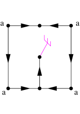
Hexagon	Square

Figure 12.6: The two types of rooted toroidal unicellular maps.

In Figure 12.7, we give several examples of executions of Algorithm PS on minimal $3$-orientations. These examples show how important is the choice of the minimal balanced Schnyder wood in order to obtain Theorem 18. In particular, the third example shows that Algorithm PS can visit all the angles of the triangulation (i.e. the cycle in the angle graph is Hamiltonian) without outputting an unicellular map.

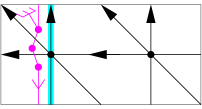
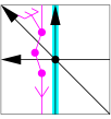
(1)	(2)

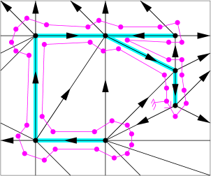
(3)

Figure 12.7: Examples of minimal $3$-orientations that are not balanced Schnyder woods and where Algorithm PS respectively: $(1)$ does not visit all the vertices, $(2)$ visits all the vertices but not all the angles, and $(3)$ visits all the angles but does not output an unicellular map.

Note that the orientations of Figure 12.7 are not Schnyder woods. One may wonder if the fact of being a Schnyder wood is of any help for our method. This is not the case since there are examples of minimal Schnyder woods that are not balanced and where Algorithm PS does not visit all the vertices. One can obtain such an example by replicating $3$ times horizontally and then $3$ times vertically the second example of Figure 12.7 to form a $3\times 3$ tiling and starts Algorithm PS from the same root angle. Conversely, there are minimal Schnyder woods that are not balanced where Algorithm PS does output a toroidal spanning unicellular map (the Schnyder wood of Figure 8.9 can serve as an example while starting from an angle of the only face oriented clockwise).

12.4 Recovering the original triangulation

This section is dedicated to showing how to recover the original triangulation from the output of Algorithm PS. The method is very similar to [45] since like in the plane the output has only one face that is homeomorphic to an open disk (i.e. a tree in the plane and an unicellular map in general).

Theorem 19

Consider a toroidal triangulation $G$, a root angle $a_{0}$ that is not in the strict interior of a separating triangle and the orientation of the edges of $G$ corresponding to the minimal balanced Schnyder wood w.r.t. the root face $f_{0}$ containing $a_{0}$. From the output $U$ of Algorithm PS applied on $(G,a_{0})$ one can reattach all the stems to obtain $G$ by starting from the root angle $a_{0}$ and walking along the face of $U$ in counterclockwise order (according to this face): each time a stem is met, it is reattached in order to create a triangular face on its left side.

Theorem 19 is illustrated on Figure 12.8 where one can check that the obtained toroidal triangulation is $K_{7}$ (like on the input of Figure 12.3).

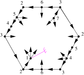
Output	Recovering

Figure 12.8: Example of how to recover the original toroidal triangulation $K_{7}$ from the output of Algorithm PS .

In fact in this section we define a method, more general than the one described in Theorem 19, that will be useful in next sections.

We consider the two type of unicellular toroidal map depicted on Figure 12.6 and call corner a vertex that is a corner of an hexagon or the square

Let $\mathcal{U}_{r}(n)$ denote the set of toroidal unicellular maps $U$ rooted on a particular angle, with exactly $n$ vertices, $n+1$ edges and $2n-1$ stems satisfying the following property. A vertex that is not the root, has exactly $2$ stems if it is not a corner, $1$ stem if it is the corner of a hexagon and $0$ stem if it is the corner of a square. The root vertex has $1$ additional stem, i.e. it has $3$ stems if it is not a corner, $2$ stems if it is the corner of a hexagon and $1$ stem if it is the corner of a square. Note that the output $U$ of Algorithm PS given by Theorem 18 is an element of $\mathcal{U}_{r}(n)$.

Similarly to the planar case [45], we define a general way to reattach step by step all the stems of an element $U$ of $\mathcal{U}_{r}(n)$. Let $U_{0}=U$, and, for $1\leq k\leq 2n-1$, let $U_{k}$ be the map obtained from $U_{k-1}$ by reattaching one of its stem (we explicit below which stem is reattached and how). The special face of $U_{0}$ is its only face. For $1\leq k\leq 2n-1$, the special face of $U_{k}$ is the face on the right of the stem of $U_{k-1}$ that is reattached to obtain $U_{k}$. For $0\leq k\leq 2n-1$, the border of the special face of $U_{k}$ consists of a sequence of edges and stems. We define an admissible triple as a sequence $(e_{1},e_{2},s)$, appearing in counterclockwise order along the border of the special face of $U_{k}$, such that $e_{1}=(u,v)$ and $e_{2}=(v,w)$ are edges of $U_{k}$ and $s$ is a stem attached to $w$. The closure of the admissible triple consists in attaching $s$ to $u$, so that it creates an edge $(w,u)$ oriented from $w$ to $u$ and so that it creates a triangular face $(u,v,w)$ on its left side. The complete closure of $U$ consists in closing a sequence of admissible triple, i.e. for $1\leq k\leq 2n-1$, the map $U_{k}$ is obtained from $U_{k-1}$ by closing any admissible triple.

Note that, for $0\leq k\leq 2n-1$, the special face of $U_{k}$ contains all the stems of $U_{k}$. The closure of a stem reduces the number of edges on the border of the special face and the number of stems by $1$. At the beginning, the unicellular map $U_{0}$ has $n+1$ edges and $2n-1$ stems. So along the border of its special face, there are $2n+2$ edges and $2n-1$ stems. Thus there is exactly three more edges than stems on the border of the special face of $U_{0}$ and this is preserved while closing stems. So at each step there is necessarily at least one admissible triple and the sequence $U_{k}$ is well defined. Since the difference of three is preserved, the special face of $U_{2n-2}$ is a quadrangle with exactly one stem. So the reattachment of the last stem creates two faces that have size three and at the end $U_{2n-1}$ is a toroidal triangulation. Note that at a given step there might be several admissible triples but their closure are independent and the order in which they are performed does not modify the obtained triangulation $U_{2n-1}$.

We now apply the closure method to our particular case. Consider a toroidal triangulation $G$, a root angle $a_{0}$ that is not in the strict interior of a separating triangle and the orientation of the edges of $G$ corresponding to the minimal balanced Schnyder wood w.r.t. the root face $f_{0}$. Let $U$ be the output of Algorithm PS applied on $(G,a_{0})$.

Lemma 56

When a stem of $U$ is reattached to form the corresponding edge of $G$, it splits the (only) face of $U$ into two faces. The root angle of $U$ is in the face that is on the right side of the stem.

Proof.  By Lemma 53, the execution of Algorithm PS corresponds to a Hamiltonian cycle $C=(a_{0},\ldots,a_{2m},a_{0})$ in the angle graph of $G$. Thus $C$ defines a total order $<$ on the angles of $G$ where $a_{i}<a_{j}$ if and only if $i<j$. Let us consider now the angles on the face of $U$. Note that such an angle corresponds to several angles of $G$, that are consecutive in $C$ and that are separated by a set of incoming edges of $G$ (those incoming edges corresponding to stems of $U$). Thus the order on the angles of $G$ defines automatically an order on the angles of $U$. The angles of $U$ considered in clockwise order along the border of its face, starting from the root angle, correspond to a sequence of strictly increasing angles for $<$.

Consider a stem $s$ of $U$ that is reattached to form an edge $e$ of $G$. Let $a_{s}$ be the angle of $U$ that is situated just before $s$ (in clockwise order along the border of the face of $U$) and $a^{\prime}_{s}$ be the angle of $U$ where $s$ should be reattached. If $a^{\prime}_{s}<a_{s}$, then when Algorithm PS consider the angle $a_{s}$, the edge corresponding to $s$ is already marked and we are not in Case 2 of Algorithm PS . So $a_{s}<a^{\prime}_{s}$ and $a_{0}$ is on the right side of $s$. $\Box$

Recall that $U$ is an element of $\mathcal{U}_{r}(n)$ so we can apply on $U$ the complete closure procedure described above. We use the same notation as before, i.e. let $U_{0}=U$ and for $1\leq k\leq 2n-1$, the map $U_{k}$ is obtained from $U_{k-1}$ by closing any admissible triple. The following lemma shows that the triangulation obtained by this method is $G$:

Lemma 57

The complete closure of $U$ is $G$, i.e. $U_{2n-1}=G$.

Proof.  We prove by induction on $k$ that every face of $U_{k}$ is a face of $G$, except for the special face. This is true for $k=0$ since $U_{0}=U$ has only one face, the special face. Let $0\leq k\leq 2n-2$, and suppose by induction that every non-special face of $U_{k}$ is a face of $G$. Let $(e_{1},e_{2},s)$ be the admissible triple of $U_{k}$ such that its closure leads to $U_{k+1}$, with $e_{1}=(u,v)$ and $e_{2}=(v,w)$. The closure of this triple leads to a triangular face $(u,v,w)$ of $U_{k+1}$. This face is the only “new” non-special face while going from $U_{k}$ to $U_{k+1}$.

Suppose, by contradiction, that this face $(u,v,w)$ is not a face of $G$. Let $a_{v}$ (resp. $a_{w}$) be the angle of $U_{k}$ at the special face, between $e_{1}$ and $e_{2}$ (resp. $e_{2}$ and $s$). Since $G$ is a triangulation, and $(u,v,w)$ is not a face of $G$, there exists at least one stem of $U_{k}$ that should be attached to $a_{v}$ or $a_{w}$ to form a proper edge of $G$. Let $s^{\prime}$ be such a stem that is the nearest from $s$. In $G$ the edges corresponding so $s$ and $s^{\prime}$ should be incident to the same triangular face. Let $x$ be the origin of the stem $s^{\prime}$. Let $z\in\{v,w\}$ such that $s^{\prime}$ should be reattached to $z$. If $z=v$, then $s$ should be reattached to $x$ to form a triangular face of $G$. If $z=w$, then $s$ should be reattached to a common neighbor of $w$ and $x$ located on the border of the special face of $U_{k}$ in counterclockwise order between $w$ and $x$. So in both cases $s$ should be reattached to a vertex $y$ located on the border of the special face of $U_{k}$ in counterclockwise order between $w$ and $x$ (with possibly $y=x$). To summarize $s$ goes from $w$ to $y$ and $s^{\prime}$ from $x$ to $z$, and $z,x,y,w$ appear in clockwise order along the special face of $U_{k}$. By Lemma 56, the root angle is on the right side of both $s$ and $s^{\prime}$, this is not possible since their right sides are disjoint, a contradiction.

So for $0\leq k\leq 2n-2$, all the non-special faces of $U_{k}$ are faces of $G$. In particular every face of $U_{2n-1}$ except one is a face of $G$. Then clearly the (triangular) special face of $U_{2n-1}$ is also a face of $G$, hence $U_{2n-1}=G$. $\Box$

Lemma 57 shows that one can recover the original triangulation from $U$ with any sequence of admissible triples that are closed successively. This does not explain how to find the admissible triples efficiently. In fact the root angle can be used to find a particular admissible triple of $U_{k}$:

Lemma 58

For $0\leq k\leq 2n-2$, let $s$ be the first stem met while walking counterclockwise from $a_{0}$ in the special face of $U_{k}$. Then before $s$, at least two edges are met and the last two of these edges form an admissible triple with $s$.

Proof.  Since $s$ is the first stem met, there are only edges that are met before $s$. Suppose by contradiction that there is only zero or one edge met before $s$. Then the reattachment of $s$ to form the corresponding edge of $G$ is necessarily such that the root angle is on the left side of $s$, a contradiction to Lemma 56. So at least two edges are met before $s$ and the last two of these edges form an admissible triple with $s$. $\Box$

Lemma 58 shows that one can reattach all the stems by walking once along the face of $U$ in counterclockwise order. Thus we obtain Theorem 19.

Note that $U$ is such that the complete closure procedure described here never wraps over the root angle, i.e. when a stem is reattached, the root angle is always on its right side (see Lemma 56). The property of never wrapping over the root angle is called safe. Usually, this property is called balanced in the literature but the word balanced is already used in this manuscript and in this chapter also. Let $\mathcal{U}_{r,s}(n)$ denote the set of elements of $\mathcal{U}_{r}(n)$ that are safe. So the output $U$ of Algorithm PS given by Theorem 18 is an element of $\mathcal{U}_{r,s}(n)$. We exhibit in Section 12.6 a bijection between appropriately rooted toroidal triangulations and a particular subset of $\mathcal{U}_{r,s}(n)$.

The possibility to close admissible triples in any order to recover the original triangulation is interesting compared to the simpler method of Theorem 19 since it enables to recover the triangulation even if the root angle is not given. This property is used in Section 12.7 to obtain a bijection between toroidal triangulations and some unrooted unicellular maps.

Moreover if the root angle is not given, then one can simply start from any angle of $U$, walk twice around the face of $U$ in counterclockwise order and reattach all the admissible triples that are encountered along this walk. Walking twice ensures that at least one complete round is done from the root angle. Since only admissible triples are considered, we are sure that no unwanted reattachment is done during the process and that the final map is $G$. This enables to reconstruct $G$ in linear time even if the root angle is not known. This property is used in Section 12.5.

12.5 Optimal encoding

The results presented in the previous sections allow us to generalize the encoding of planar triangulations, defined by Poulalhon and Schaeffer [45], to triangulations of the torus. The construction is direct and it is hence really different from the one of [14] where triangulations of surfaces are cut in order to deal with planar triangulations with boundaries. Here we encode the unicellular map outputted by Algorithm PS by a plane rooted tree with $n$ vertices and with exactly two stems attached to each vertex, plus $O(\log(n))$ bits. As in [14], this encoding is asymptotically optimal and uses approximately $3.2451n$ bits. The advantage of our method is that it can be implemented in linear time. Moreover we believe that our encoding gives a better understanding of the structure of triangulations of the torus. It is illustrated with new bijections that are obtained in Sections 12.6 and 12.7.

Consider a toroidal triangulation $G$, a root angle $a_{0}$ that is not in the strict interior of a separating triangle and the orientation of the edges of $G$ corresponding to the minimal balanced Schnyder wood w.r.t. the root face $f_{0}$. Let $U$ be the output of Algorithm PS applied on $(G,a_{0})$. As already mentioned at the end of Section 12.4, to retrieve the triangulation $G$ one just needs to know $U$ without the information of its root angle (by walking twice around the face of $U$ in counterclockwise order and reattaching all the admissible triples that are encountered along this walk, one can recover $G$). Hence to encode $G$, one just has to encode $U$ without the position of the root angle around the root vertex (see Figure 12.9.(a)).

By Lemma 51, the unicellular map $U$ contains a spanning tree $T$ which is oriented from the leaves to the root vertex. The tree $T$ contains exactly $n-1$ edges, so there is exactly $2$ edges of $U$ that are not in $T$. We call these edges the special edges of $U$. We cut these two special edges to transform them into stems of $T$ (see Figures 12.9.(a) and (b)). We keep the information of where are the special stems in $T$ and on which angle of $T$ they should be reattached. This information can be stored with $O(\log(n))$ bits. One can recover $U$ from $T$ by reattaching the special stems in order to form non-contractible cycles with $T$ (see Figure 12.9.(c)).

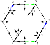
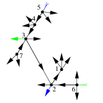
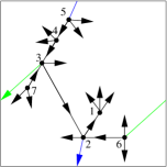
(a)	(b)	(c)

Figure 12.9: From unicellular maps to trees with special stems and back.

So $T$ is a plane tree on $n$ vertices, each vertex having $2$ stems except the root vertex $v_{0}$ having three stems. Choose any stem $s_{0}$ of the root vertex, remove it and consider that $T$ is rooted at the angle where $s_{0}$ should be attached. The information of the root enables to put back $s_{0}$ at its place. So now we are left with a rooted plane tree $T$ on $n$ vertices where each vertex has exactly $2$ stems (see Figure 12.10.(a)).

This tree $T$ can easily be encoded by a binary word on $6n-2$ bits: that is, walking in counterclockwise order around $T$ from the root angle, writing a “1” when going down along $T$, and a “0” when going up along $T$ (see Figure 12.10.(a)). As in [45], one can encode $T$ more compactly by using the fact that each vertex has exactly two stems. Thus $T$ is encoded by a binary word on $4n-2$ bits: that is, walking in counterclockwise order around $T$ from the root angle, writing a “1” when going down along an edge of $T$, and a “0” when going up along an edge or along a stem of $T$ (see Figure 12.10.(b) where the “red 1’s” of Figure 12.10.(a) have been removed). Indeed there is no need to encode when going down along stems, this information can be retrieved afterward. While reading the binary word to recover $T$, when a “0” is met, we should go up in the tree, except if the vertex that we are considering does not have already its two stems, then in that case we should create a stem (i.e. add a “red 1” before the “0”). So we are left with a binary word on $4n-2$ bits with exactly $n-1$ bits “1” and $3n-1$ bits “0”.

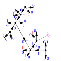
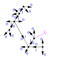
1010111011101001010010110100010101101000	00110110000000100000010000
(a)	(b)

Figure 12.10: Encoding a rooted tree with two stems at each vertex.

Similarly to [45], using [9, Lemma 7], this word can then be encoded with a binary word of length $\log_{2}\binom{4n-2}{n-1}+o(n)\sim n\,\log_{2}(\frac{256}{27})\approx 3.2451\,n$ bits. Thus we have the following theorem whose linearity is discussed below:

Theorem 20

Any toroidal triangulation on $n$ vertices, can be encoded with a binary word of length $3.2451n+o(n)$ bits, the encoding and decoding being linear in $n$.

The encoding method described here, that is encoding a toroidal triangulation via an unicellular map and recovering the original triangulation, can be performed in linear time. The only difficulty lies in providing Algorithm PS with the appropriate input it needs in order to apply Theorem 18. Then clearly the execution of Algorithm PS, the encoding phase and the recovering of the triangulation are linear like in the planar case. Thus we have to show how one can find in linear time a root angle $a_{0}$ that is not in the strict interior of a separating triangle, as well as the minimal balanced Schnyder wood w.r.t. the root face $f_{0}$.

Consider a balanced Schnyder wood of $G$ that can be computed in linear time as explained in Section 10.1. From this balanced Schnyder wood, one can compute in linear time a root angle $a_{0}$ not in the strict interior of a separating triangle. First note that in a $3$-orientation of a toroidal triangulation, the edges that are inside a separating triangle and that are incident to the three vertices on the border are all oriented toward these three vertices by Euler’s formula. Thus an oriented non-contractible cycle cannot enter in the interior of a separating triangle. Now follow any oriented monochromatic path of the Schnyder wood and stop the first time this path is back to a previously met vertex $v_{0}$. The end of this path forms an oriented monochromatic cycle $C$ containing $v_{0}$. Thus $C$ is an oriented non-contractible cycle and cannot contain some vertices that are in the interior of a separating triangle. So $v_{0}$ is not in the interior of a separating triangle and we can choose as root angle $a_{0}$ any angle incident to $v_{0}$. Then using the method described in Section 5.2. one can transform the balanced Schnyder wood of $G$ into a minimal balanced Schnyder wood w.r.t. the root face $f_{0}$.

12.6 Bijection with rooted unicellular maps

Given a toroidal triangulation $G$ with a root angle $a_{0}$, we have defined a unique associated orientation: the minimal balanced Schnyder wood w.r.t. the root face $f_{0}$. Suppose that $G$ is oriented according to the minimal balanced Schnyder wood. If $a_{0}$ is not in the strict interior of a separating triangle then Theorems 18 and 19 show that the execution of Algorithm PS on $(G,a_{0})$ gives a toroidal unicellular map with stems from which one can recover the original triangulation. Thus there is a bijection between toroidal triangulations rooted from an appropriate angle and their image by Algorithm PS. The goal of this section is to describe this image.

Recall from Section 12.4 that the output of Algorithm PS on $(G,a_{0})$ is an element of $\mathcal{U}_{r,s}(n)$. One may hope that there is a bijection between toroidal triangulations rooted from an appropriate angle and $\mathcal{U}_{r,s}(n)$ since this is how it works in the planar case. Indeed, given a planar triangulation $G$, there is a unique orientation of $G$ (the minimal Schnyder wood) on which Algorithm PS, performed from an outer angle, outputs a spanning tree. In the toroidal case, things are more complicated since the behavior of Algorithm PS on minimal balanced Schnyder woods does not characterize such orientations.

Figure 12.11 gives an example of two (non homologous) orientations of the same triangulation that are both minimal w.r.t. the same root face. For these two orientations, the execution of Algorithm PS from the same root angle gives two different elements of $\mathcal{U}_{r,s}(2)$ (from which the original triangulation can be recovered by the method of Theorem 19).

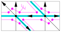
balanced orientation	non-balanced orientation

Figure 12.11: A graph that can be represented by two different unicellular maps.

Let us translate the balanced property on $\mathcal{U}_{r}(n)$. Consider an element $U$ of $\mathcal{U}_{r}(n)$ whose edges and stems are oriented w.r.t. the root angle as follows: the stems are all outgoing, and while walking clockwise around the unique face of $U$ from $a_{0}$, the first time an edge is met, it is oriented counterclockwise w.r.t. the face of $U$. Then one can compute $\gamma$ (define in Section 4.2) on the cycles of $U$ (edges and stems count). We say that an unicellular map of $\mathcal{U}_{r}(n)$ satisfies the $\gamma_{0}$ property if $\gamma$ equals zero on its (non-contractible) cycles. Let us call $\mathcal{U}_{r,s,\gamma_{0}}(n)$ the set of elements of $\mathcal{U}_{r,s}(n)$ satisfying the $\gamma_{0}$ property. So the output of Algorithm PS given by Theorem 18 is an element of $\mathcal{U}_{r,s,\gamma_{0}}(n)$.

Let $\mathcal{T}_{r}(n)$ be the set of toroidal triangulations on $n$ vertices rooted at an angle that is not in the strict interior of a separating triangle. Then we have the following bijection:

Theorem 21

There is a bijection between $\mathcal{T}_{r}(n)$ and $\mathcal{U}_{r,s,\gamma_{0}}(n)$.

Proof.  Consider the mapping $g$ that associates to an element of $\mathcal{T}_{r}(n)$, the output of Algorithm PS executed on the minimal balanced Schnyder wood w.r.t. the root face. By the above discussion the image of $g$ is in $\mathcal{U}_{r,s,\gamma_{0}}(n)$ and $g$ is injective since one can recover the original triangulation from its image by Theorem 19.

Conversely, given an element $U$ of $\mathcal{U}_{r,s,\gamma_{0}}(n)$ with root angle $a_{0}$, one can build a toroidal map $G$ by the complete closure procedure described in Section 12.4. The number of stems and edges of $U$ implies that all faces of $G$ are triangles. We explain below why $G$ has no contractible loop nor multiple edges. Recall that $a_{0}$ defines an orientation on the edges and stems of $U$. Consider the orientation $D$ of $G$ induced by this orientation. Since $U$ is safe, the execution of Algorithm PS on $(G,a_{0})$ corresponds to the cycle in the angle graph of $U$ obtained by starting from the root angle and walking clockwise in the face of $U$. Thus the output of Algorithm PS executed on $(G,a_{0})$ is $U$. First note that by definition of $\mathcal{U}_{r}(n)$, the orientation $D$ is a $3$-orientation. Thus a simple counting argument shows that $G$ has no contractible loop nor multiple edges. It remains to show that $G$ is appropriately rooted and that $D$ corresponds to the minimal balanced Schnyder wood w.r.t. this root.

First note that by definition of $\mathcal{U}_{r}(n)$, the orientation $D$ is a $3$-orientation.

Suppose by contradiction that $a_{0}$ is in the strict interior of a separating triangle. Then, since we are considering a $3$-orientation, by Euler’s formula, the edges in the interior of this triangle and incident to its border are all entering the border. So Algorithm PS starting from the strict interior cannot visit the vertices on the border of the triangle and outside. Thus the output of Algorithm PS is not a toroidal unicellular map, a contradiction. So $a_{0}$ is not in the strict interior of a separating triangle.

The $\gamma_{0}$ property of $U$ implies that $\gamma$ equals zero on two cycles of $U$. Hence these two cycles considered in $G$ also satisfy $\gamma$ equals $0$ so $D$ is a balanced Schnyder wood by Lemma 34.

Suppose by contradiction that $D$ is not minimal. We use the terminology and notations of Section 5.2. Then $D$ contains a clockwise (non-empty) $0$-homologous oriented subgraph w.r.t. $f_{0}$. Let $T$ be such a subgraph with $\phi(T)=-\sum_{F\in\mathcal{F}^{\prime}}\lambda_{F}\phi(F)$, with $\lambda\in\mathbb{N}^{|\mathcal{F}^{\prime}|}$. Let $\lambda_{f_{0}}=0$, and $\lambda_{\max}=\max_{F\in\mathcal{F}}\lambda_{F}$. For $0\leq i\leq\lambda_{\max}$, let $X_{i}=\{F\in\mathcal{F}\,|\,\lambda_{F}\geq i\}$. For $1\leq i\leq\lambda_{\max}$, let $T_{i}$ be the oriented subgraph such that $\phi(T_{i})=-\sum_{F\in X_{i}}\phi(F)$. Then we have $\phi(T)=\sum_{1\leq i\leq\lambda_{\max}}\phi(T_{i})$. Since $T$ is an oriented subgraph, we have $\phi(T)\in\{-1,0,1\}^{|E(G)|}$. Thus for any edge of ${G}$, incident to faces $F_{1}$ and $F_{2}$, we have $(\lambda_{F_{1}}-\lambda_{F_{2}})\in\{-1,0,1\}$. So, for $1\leq i\leq\lambda_{\max}$, the oriented graph $T_{i}$ is the frontier between the faces with $\lambda$ value equal to $i$ and $i-1$. So all the $T_{i}$ are edge disjoint and are oriented subgraphs of $D$. Since $T$ is non-empty, we have $\lambda_{\max}\geq 1$, and $T_{1}$ is non-empty. All the edges of $T_{1}$ have a face of $X_{1}$ on their right and a face of $X_{0}$ on their left. Since $U$ is an unicellular map, and $T_{1}$ is a (non-empty) $0$-homologous oriented subgraph, at least one edge of $T_{1}$ corresponds to a stem of $U$. Let $s$ be the last stem of $U$ corresponding to an edge of $T_{1}$ that is reattached by the complete closure procedure. Consider the step where $s$ is reattached. As the root angle (and thus $f_{0}$) is in the special face (see the terminology of Section 12.4), the special face is in the region defined by $X_{0}$. Thus it is on the left of $s$ when it is reattached. This contradicts the fact that $U$ is safe. Thus $D$ is the minimal balanced Schnyder wood w.r.t. $f_{0}$. $\Box$

12.7 Bijection with unrooted unicellular maps

The goal of this section is to remove the root and the safe property of the unicellular maps considered in Theorem 21. For this purpose, we have to root the toroidal triangulation more precisely than before. We say that an angle is not in the clockwise interior of a separating triangle if it is not in its interior, or if it is incident to a vertex $v$ of the triangle and situated just before an edge of the triangle in counterclockwise order around $v$ (see Figure 12.12).

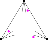
Figure 12.12: Angles that are in a separating triangle but not in its clockwise interior.

Consider a toroidal triangulation $G$. Consider a root angle $a_{0}$ that is not in the clockwise interior of a separating triangle. Note that the choice of $a_{0}$ is equivalent to the choice of a root vertex $v_{0}$ and a root edge $e_{0}$ incident to $v_{0}$ such that none is in the interior of a separating triangle. Consider the orientation of the edges of $G$ corresponding to the minimal balanced Schnyder wood w.r.t. the root face $f_{0}$. By Lemma 39, there is a clockwise triangle containing $f_{0}$. Thus by the choice of $a_{0}$, the edge $e_{0}$ is leaving the root vertex $v_{0}$. This is the essential property used in this section. Consider the output $U$ of Algorithm PS on $(G,a_{0})$. Since $e_{0}$ is leaving $v_{0}$ and $a_{0}$ is just before $e_{0}$ in counterclockwise order around $v_{0}$, the execution of Algorithm PS starts by Case 2 and $e_{0}$ corresponds in $U$ to a stem $s_{0}$ attached to $v_{0}$. We call this stem $s_{0}$ the root stem.

The recovering method defined in Theorem 19 says that $s_{0}$ is the last stem reattached by the procedure. So there exists a sequence of admissible triples of $U$ (see the terminology and notations of Section 12.4) such that $s_{0}$ belongs to the last admissible triple. Let $U_{0}=U$ and for $1\leq k\leq 2n-2$, the map $U_{k}$ is obtained from $U_{k-1}$ by closing any admissible triple that does no contain $s_{0}$. As noted in Section 12.4, the special face of $U_{2n-2}$ is a quadrangle with exactly one stem. This stem being $s_{0}$, we are in the situation of Figure 12.13.

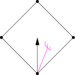
Figure 12.13: The situation just before the last stem (i.e. the root stem) is reattached

Consequently, if one removes the root stem $s_{0}$ from $U$ to obtain an unicellular map $U^{\prime}$ with $n$ vertices, $n+1$ edges and $2n-2$ stems, one can recover the graph $U_{2n-2}$ by applying a complete closure procedure on $U^{\prime}$ (see example of Figure 12.14). Note that then, there are four different ways to finish the closure of $U_{2n-2}$ to obtain an oriented toroidal triangulation. This four cases correspond to the four ways to place the (removed) root stem in a quadrangle, they are obtained by pivoting Figure 12.13 by 0°, 90°, 180° and 270°. Note that only one of this four cases leads to the original rooted triangulation $G$, except if there are some symmetries (like in the example of Figure 12.14).

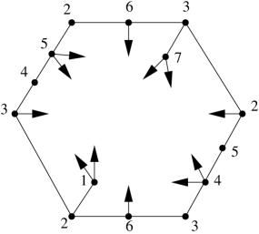
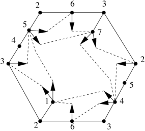
Non-rooted output	Partial recovering

Figure 12.14: Example of $K_{7}$ where the root angle, the root stem and the orientation w.r.t. the root angle have been removed from the output of Figure 12.3. The complete closure procedure leads to a quadrangular face.

Let $\mathcal{U}(n)$ denote the set of (non-rooted) toroidal unicellular maps, with exactly $n$ vertices, $n+1$ edges and $2n-2$ stems satisfying the following: a vertex has exactly $2$ stems if it is not a corner, $1$ stem if it is the corner of a hexagon and $0$ stem if it is the corner of a square. Note that the output of Theorem 18 on an appropriately rooted toroidal triangulation is an element of $\mathcal{U}(n)$ when the root stem is removed.

Note that an element $U^{\prime}$ of $\mathcal{U}(n)$ is non-rooted so we cannot orient automatically its edges w.r.t. the root angle like in Section 12.6. Nevertheless one can still orient all the stems as outgoing and compute $\gamma$ on the cycles of $U^{\prime}$ by considering only its stems in the counting (and not the edges nor the root stem anymore). We say that an unicellular map of $\mathcal{U}(n)$ satisfies the $\gamma_{0}$ property if $\gamma$ equals zero on its (non-contractible) cycles. Let us call $\mathcal{U}_{\gamma_{0}}(n)$ the set of elements of $\mathcal{U}(n)$ satisfying the $\gamma_{0}$ property.

A surprising property is that an element $U^{\prime}$ of $\mathcal{U}(n)$ satisfies the $\gamma_{0}$ property if and only if any element $U$ of $\mathcal{U}_{r}(n)$ obtained from $U^{\prime}$ by adding a root stem anywhere in $U^{\prime}$ satisfies the $\gamma_{0}$ property (note that in $U$ we count the edges and the root stem to compute $\gamma$). One can see this by considering the unicellular map of Figure 12.15. It represents the general case of the underlying rooted hexagon of $U$. The edges represent in fact paths (some of which can be of length zero). One can check that it satisfies $\gamma$ equals zero on its (non-contractible) cycles. It corresponds exactly to the set of edges that are taken into consideration when computing $\gamma$ on $U$ but not when computing $\gamma$ on $U^{\prime}$. Thus it does not affect the counting (the tree-like parts are not represented since they do not affect the value $\gamma$). So the output of Theorem 18 on an appropriately rooted toroidal triangulation is an element of $\mathcal{U}_{\gamma_{0}}(n)$ when the root stem is removed.

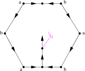
Figure 12.15: The parts of the unicellular map showing the correspondence while computing $\gamma$ with or without the orientation w.r.t. the root plus the root stem.

For the particular case of $K_{7}$, the difference between the rooted output of Figure 12.3 and the non-rooted output of Figure 12.14 is represented on Figure 12.16 (one can superimpose the last two to obtain the first). One can check that these three unicellular maps (rooted, non-rooted and the difference) all satisfy $\gamma$ equals zero on their cycles.

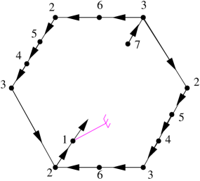
Figure 12.16: The difference between the rooted output of Figure 12.3 and the non-rooted output of Figure 12.14.

There is an “almost” four-to-one correspondence between toroidal triangulations on $n$ vertices, given with a root angle that is not in the clockwise interior of a separating triangle, and elements of $\mathcal{U}_{\gamma_{0}}(n)$. The “almost” means that if the automorphism group of an element $U$ of $\mathcal{U}_{\gamma_{0}}(n)$ is not trivial, some of the four ways to add a root stem in $U$ are isomorphic and lead to the same rooted triangulation. In the example of Figure 12.14, one can root in four ways the quadrangle but this gives only two different rooted triangulations (because of the symmetries of $K_{7}$). We face this problem by defining another class for which we can formulate a bijection.

Let $\mathcal{T}(n)$ be the set of toroidal maps on $n$ vertices, where all the faces are triangles, except one that is a quadrangle and which is not in a separating triangle. Then we have the following bijection:

Theorem 22

There is a bijection between $\mathcal{T}(n)$ and $\mathcal{U}_{\gamma_{0}}(n)$.

Proof.  Let $a$ (for “add”) be an arbitrarily chosen mapping defined on the maps $G^{\prime}$ of $\mathcal{T}(n)$ that adds a diagonal $e_{0}$ in the quadrangle of $G^{\prime}$ and roots the obtained toroidal triangulation $G$ at a vertex $v_{0}$ incident to $e_{0}$ (this defines the root angle $a_{0}$ situated just before $e_{0}$ in counterclockwise order around $v_{0}$). Note that the added edge cannot create homotopic multiple edges, since otherwise the quadrangle would be in a separating triangle. Moreover the root angle of $G$ is not in the clockwise interior of a separating triangle. Thus the image of $a$ is in $\mathcal{T}^{\prime}_{r}(n)$, the subset of $\mathcal{T}_{r}(n)$ corresponding to toroidal triangulations rooted at an angle that is not in the clockwise interior of a separating triangle.

Let $\mathcal{U}^{\prime}_{r,s,\gamma_{0}}(n)$ be the elements of $\mathcal{U}_{r,s,\gamma_{0}}(n)$ that have their root angle just before a stem in counterclockwise order around the root vertex. Consider the mapping $g$, defined in the proof of Theorem 21. By Lemma 39 and Theorem 21, the image of $g$ restricted to $\mathcal{T}^{\prime}_{r}(n)$ is in $\mathcal{U}^{\prime}_{r,s,\gamma_{0}}(n)$. Let $r$ (for “remove”) be the mapping that associates to an element of $\mathcal{U}^{\prime}_{r,s,\gamma_{0}}(n)$ an element of $\mathcal{U}_{\gamma_{0}}(n)$ obtained by removing the root angle and its corresponding stem. Finally, let $h=r\circ g\circ a$ which associates to an element of $\mathcal{T}(n)$ an element of $\mathcal{U}_{\gamma_{0}}(n)$. Let us show that $h$ is a bijection.

Consider an element $G^{\prime}$ of $\mathcal{T}(n)$ and its image $U^{\prime}$ by $h$. The complete closure procedure on $U^{\prime}$ gives $G^{\prime}$ thus the mapping $h$ is injective.

Conversely, consider an element $U^{\prime}$ of $\mathcal{U}_{\gamma_{0}}(n)$. Apply the complete closure procedure on $U^{\prime}$. At the end of this procedure, the special face is a quadrangle whose angles are denoted $\alpha^{1},\ldots,\alpha^{4}$. We denote also by $\alpha^{1},\ldots,\alpha^{4}$ the corresponding angles of $U^{\prime}$. For $i\in\{1,\ldots,4\}$, let $U^{i}$ be the element of $\mathcal{U}_{r}(n)$ obtained by adding a root stem and a root angle in the angle $\alpha^{i}$ of $U^{\prime}$, with the root angle just before the stem in counterclockwise order around the root vertex. Note that by the choice of $\alpha^{i}$, the $U^{i}$ are all safe. By above remarks they also satisfy the $\gamma_{0}$ property and thus they are in $\mathcal{U}^{\prime}_{r,s,\gamma_{0}}(n)$.

By the proof of Theorem 21, the complete closure procedure on $U^{i}$ gives a triangulation $G^{i}$ of $\mathcal{T}_{r}(n)$ that is rooted from an angle $a_{0}^{i}$ not in the strict interior of a separating triangle and oriented according to the minimal balanced Schnyder wood w.r.t. the root face. Moreover the output of Algorithm PS applied on $(G^{i},a_{0}^{i})$ is $U^{i}$. Since in $U^{i}$, the root stem is present just after the root angle, the first edge seen by the execution of Algorithm PS on $(G^{i},a_{0}^{i})$ is outgoing. So $a_{0}$ is not in the clockwise interior of a separating triangle (in a $3$-orientation, all the edges that are in the interior of a separating triangle and incident to the triangle are entering the triangle). Thus the $G^{i}$ are appropriately rooted and are elements of $\mathcal{T}^{\prime}_{r}(n)$. Removing the root edge of any $G^{i}$, gives the same map $G^{\prime}$ of $\mathcal{T}(n)$. Exactly one of the $G^{i}$ is the image of $G^{\prime}$ by the mapping $a$. Thus the image of $G^{\prime}$ by $h$ is $U^{\prime}$ and the mapping $h$ is surjective. $\Box$

A nice aspect of Theorem 22 comparing to Theorem 21 is that the unicellular maps that are considered are much simpler. They have no root nor safe property anymore.

12.8 Conjecture for higher genus

Note that the work presented here is related to a work of Bernardi and Chapuy [7] (their convention for the orientation of the edges is the reverse of ours). Consider a map $G$ (not necessarily a triangulation) on an orientable surface of genus $g$, rooted at a particular angle $a_{0}$. An orientation of $G$ is right if for each edge $e$, the right-walk starting from $e$ (when entering a vertex, the next chosen edge is the one leaving on the right) reaches the root edge $e_{0}$ via the root vertex $v_{0}$. A consequence of [7] is that Algorithm PS applied on an orientation of $(G,a_{0})$ outputs a spanning unicellular submap $U$ if and only if the considered orientation is right. Note that in this characterization, the submap $U$ is not necessarily a map of genus $g$, its genus can be any value in $\{0,\ldots,g\}$. In the particular case of toroidal triangulations we show that by considering minimal balanced Schnyder woods the output $U$ is a toroidal spanning unicellular map. Hence by the above characterization, minimal balanced Schnyder woods are right. But here, the fact that $U$ and $G$ have the same genus is of particular interest as it yields a simple bijection.

The key property that makes $U$ and $G$ have same genus is the conclusion of Lemma 36 (no oriented non-contractible cycle in the dual orientation). Thus we we hope for a possible generalization of Theorem 3 satisfying the conclusion of Lemma 36:

Conjecture 3

A triangulation on a genus $g\geq 1$ orientable surface admits an orientation of its edges such that every vertex has outdegree at least $3$, divisible by $3$, and such that there is no oriented non-contractible cycle in the dual orientation.

If Conjecture 3 is true, one can consider a minimal orientation satisfying its conclusion and apply Algorithm PS to obtain a unicellular map of the same genus as $G$. Note that more efforts should be made to obtain a bijection since there might be several minimal elements satisfying the conjecture and a particular one has to be identified (as the minimal balanced Schnyder wood in our case).

Chapter 13 Orthogonal surfaces and straight-line drawing

13.1 Periodic geodesic embedding

Generalizing results for planar maps [11, 22, 41], we show that Schnyder woods can be used to embed the universal cover of an essentially 3-connected toroidal map on an infinite and periodic orthogonal surface. This embedding is then used to obtain a straight-line flat torus representation of any toroidal map in a polynomial size grid.

Given two points $u=(u_{0},u_{1},u_{2})$ and $v=(v_{0},v_{1},v_{2})$ in $\mathbb{R}^{3}$, we note $u\vee v=(\max(u_{i},v_{i}))_{i=0,1,2}$ and $u\wedge v=(\min(u_{i},v_{i}))_{i=0,1,2}$. We define an order $\geq$ among the points in $\mathbb{R}^{3}$, in such a way that $u\geq v$ if $u_{i}\geq v_{i}$ for $i=0,1,2$.

Given a set $\mathcal{V}$ of pairwise incomparable elements in $\mathbb{R}^{3}$, we define the set of vertices that dominates $\mathcal{V}$ as $\mathcal{D}_{\mathcal{V}}=\{u\in\mathbb{R}^{3}\ |\ \exists\,v\in\mathcal{V}$ such that $u\geq v\}$. The orthogonal surface $\mathcal{S}_{\mathcal{V}}$ generated by $\mathcal{V}$ is the boundary of $\mathcal{D}_{\mathcal{V}}$. (Note that orthogonal surfaces are well defined even when $\mathcal{V}$ is an infinite set.) If $u,v\in\mathcal{V}$ and $u\vee v\in\mathcal{S}_{\mathcal{V}}$, then $\mathcal{S}_{\mathcal{V}}$ contains the union of the two line segments joining $u$ and $v$ to $u\vee v$. Such arcs are called elbow geodesic. The orthogonal arc of $v\in\mathcal{V}$ in the direction of the standard basis vector $e_{i}$ is the intersection of the ray $v+\lambda e_{i}$ with $\mathcal{S}_{\mathcal{V}}$.

Let $G$ be a planar map. A geodesic embedding of $G$ on the orthogonal surface $\mathcal{S}_{\mathcal{V}}$ is a drawing of $G$ on $\mathcal{S}_{\mathcal{V}}$ satisfying the following:

• There is a bijection between the vertices of $G$ and $\mathcal{V}$.

• Every edge of $G$ is an elbow geodesic.

• Every orthogonal arc in $\mathcal{S}_{\mathcal{V}}$ is part of an edge of $G$.

• There are no crossing edges in the embedding of $G$ on $\mathcal{S}_{\mathcal{V}}$.

Miller [41] (see also [22, 26]) proved that a geodesic embedding of a planar map $G$ on an orthogonal surface $\mathcal{S}_{\mathcal{V}}$ induces a planar Schnyder wood of $G$. The edges of $G$ are colored with the direction of the orthogonal arc contained in the edge. An orthogonal arc intersecting the ray $v+\lambda e_{i}$ corresponds to the edge leaving $v$ in color $i$. Edges represented by two orthogonal arcs correspond to edges oriented in two directions.

Conversely, it has been proved that a Schnyder wood of a planar map $G$ can be used to obtain a geodesic embedding of $G$. Let $G$ be a planar map given with a Schnyder wood. The method is the following (see [22] for more details): For every vertex $v$, one can divide $G$ into the three regions bounded by the three monochromatic paths going out from $v$ (see Figure 2.4). The region vector associated to $v$ is the vector obtained by counting the number of faces in each of these three regions. The mapping of each vertex on its region vector gives the geodesic embedding. Note that in this approach, the vertices are all mapped on the same plane as the sum of the coordinates of each region vector is equal to the total number of inner faces of the map.

Our goal is to generalize geodesic embeddings to the torus. More precisely, we want to represent the universal cover of a toroidal map on an infinite and periodic orthogonal surface.

Let $G$ be a toroidal map. Consider a representation of $G$ in a parallelogram $P$ whose opposite sides are identified. The graph $G^{\infty}$ is obtained by replicating $P$ to tile the plane. Given any parallelogram $Q$ representing a copy of $G$ in $G^{\infty}$, we choose arbitrarily two consecutive sides of $Q$ in clockwise order and say that the first one is the top side and the second one is the right side. Let $Q^{top}$ (resp. $Q^{right}$) be the copy of $Q$ just above (resp. on the right of) $Q$, w.r.t. the top and right side of $Q$. Given a vertex $v$ in $Q$, we note $v^{top}$ (resp. $v^{right}$) its copies in $Q^{top}$ (resp. $Q^{right}$).

A mapping of the vertices of $G^{\infty}$ in $\mathbb{R}^{d}$, $d\in\{2,3\}$, is periodic with respect to vectors $S$ and $S^{\prime}$ of $\mathbb{R}^{d}$, if there exists a parallelogram $Q$ representing a copy of $G$ in $G^{\infty}$ such that for any vertex $v$ of $G^{\infty}$, vertex $v^{top}$ is mapped on $v+S$ and $v^{right}$ is mapped on $v+S^{\prime}$. A geodesic embedding of a toroidal map $G$ is a geodesic embedding of $G^{\infty}$ on $\mathcal{S}_{\mathcal{V}^{\infty}}$, where $\mathcal{V}^{\infty}$ is a periodic mapping of $G^{\infty}$ w.r.t. two non collinear vectors.

The goal of the next two sections is to prove the following theorem (see example of Figure 13.1, where the black parallelogram represents a copy of the map that is the basic tile used to fill the plane):

Theorem 23

The universal cover of an essentially 3-connected toroidal map admits a geodesic embedding on an infinite and periodic orthogonal surface.

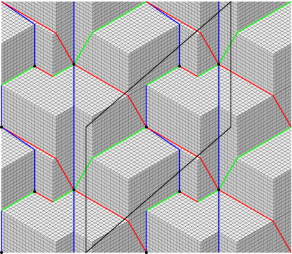
Figure 13.1: Geodesic embedding of the toroidal map of Figure 3.12.

13.2 Generalization of the region vector

Like in the plane, Schnyder woods can be used to obtain geodesic embeddings of toroidal maps. For that purpose, we need to generalize the region vector method. The idea is to use the regions to compute the coordinates of the vertices of the universal cover. The problem is that contrarily to the planar case, these regions are unbounded and contains an infinite number of faces. The method is thus generalized by the following.

Consider a toroidal map $G$ given with an intersecting Schnyder wood. We say that the Schnyder wood is of type 1 if it is crossing and type 2 if it is not crossing. When it is not crossing, we may specify the only color $i$ for which it is $i$-crossing (see Theorem 9) by saying that the Schnyder wood is of type 2.i.

Recall that $\mathcal{C}_{i}$ denotes the set of $i$-cycles of $G$. The Schnyder wood is intersecting so, by Theorem 9, the cycles of $\mathcal{C}_{i}$ are non-contractible, non intersecting and homologous. So we can order them as follows $\mathcal{C}_{i}=\{C_{i}^{0},\ldots,C_{i}^{k_{i}-1}\}$, $k_{i}\geq 1$, such that, for $0\leq j\leq k_{i}-1$, there is no $i$-cycle in the region $R(C_{i}^{j},C_{i}^{j+1})$ between $C_{i}^{j}$ and $C_{i}^{j+1}$ containing the right side of $C_{i}^{j}$ (superscript understood modulo $k_{i}$). Recall that if the Schnyder wood is of type 2.i, then $\mathcal{C}_{i-1}=(\mathcal{C}_{i+1})^{-1}$ by Theorem 9.

A directed monochromatic cycle $C_{i}^{j}$ corresponds to a family of $i$-lines of $G^{\infty}$, denoted $\mathcal{L}_{i}^{j}$. Given any two $i$-lines $L$, $L^{\prime}$, the unbounded region between $L$ and $L^{\prime}$ is noted $R(L,L^{\prime})$. We say that two $i$-lines $L,L^{\prime}$ are consecutive if there is no $i$-line contained in $R(L,L^{\prime})$. The positive side of a $i$-line is defined as the right side while “walking” along the directed path by following the orientation of the edges colored $i$.

Lemma 59

For any vertex $v$, the two monochromatic lines $L_{i-1}(v)$ and $L_{i+1}(v)$ intersect. Moreover, if the Schnyder wood is of type 2.i, then $L_{i+1}(v)=(L_{i-1}(v))^{-1}$ and $v$ is situated on the right of $L_{i+1}(v)$.

Proof.  Let $j,j^{\prime}$ be such that $L_{i-1}(v)\in\mathcal{L}_{i-1}^{j}$ and $L_{i+1}(v)\in\mathcal{L}_{i+1}^{j^{\prime}}$. If the Schnyder wood is of type 1 or type 2.j with $j\neq i$, then the two cycles $C_{i-1}^{j}$ and $C_{i+1}^{j^{\prime}}$ are crossing, and so the two lines $L_{i-1}(v)$ and $L_{i+1}(v)$ intersect.

Suppose now that the Schnyder wood is of type 2.i. If $v\in L_{i-1}(v)$, then clearly $L_{i+1}(v)=(L_{i-1}(v))^{-1}$ and $v\in L_{i+1}(v)$. The case where $v\in L_{i+1}(v)$ is similar and we can assume now that $v$ does not belong to $L_{i-1}(v)$ nor $L_{i+1}(v)$. Then $v$ lies between two consecutive $(i+1)$-lines (which are also $(i-1)$-lines). Let us denote those two lines $L_{i+1}$ and $L^{\prime}_{i+1}$, such that $L^{\prime}_{i+1}$ is situated on the right of $L_{i+1}$. By the Schnyder property, paths $P_{i+1}(v)$ and $P_{i-1}(v)$ cannot reach $L^{\prime}_{i+1}$. Thus $L_{i+1}=L_{i+1}(v)=(L_{i-1}(v))^{-1}$. $\Box$

The size of the region $R(C_{i}^{j},C_{i}^{j+1})$ of $G$, denoted $f_{i}^{j}=|R(C_{i}^{j},C_{i}^{j+1})|$, is equal to the number of faces in $R(C_{i}^{j},C_{i}^{j+1})$. Remark that for each color, we have $\sum_{j=0}^{k_{i}-1}f_{i}^{j}$ equals the total number of faces $f$ of $G$. If $L$ and $L^{\prime}$ are consecutive $i$-lines of $G^{\infty}$ with $L\in\mathcal{L}_{i}^{j}$ and $L^{\prime}\in\mathcal{L}_{i}^{j+1}$, then the size of the (unbounded) region $R(L,L^{\prime})$, denoted $|R(L,L^{\prime})|$, is equal to $f_{i}^{j}$. If $L$ and $L^{\prime}$ are any $i$-lines, the size of the (unbounded) region $R(L,L^{\prime})$, denoted $|R(L,L^{\prime})|$, is equal to the sum of the size of all the regions delimited by consecutive $i$-lines inside $R(L,L^{\prime})$. For each color $i$, choose arbitrarily a $i$-line $L_{i}^{*}$ in $\mathcal{L}_{i}^{0}$ that is used as an origin for $i$-lines. Given a $i$-line $L$, we define the value $f_{i}(L)$ of $L$ as follows: $f_{i}(L)=|R(L,L_{i}^{*})|$ if $L$ is on the positive side (right side) of $L_{i}^{*}$ and $f_{i}(L)=-|R(L,L_{i}^{*})|$ otherwise.

Consider two vertices $u,v$ such that $L_{i-1}(u)=L_{i-1}(v)$ and $L_{i+1}(u)=L_{i+1}(v)$. Even if the two regions $R_{i}(u)$ and $R_{i}(v)$ are unbounded, their difference is bounded. Let $d_{i}(u,v)$ be the number of faces in $R_{i}(u)\setminus R_{i}(v)$ minus the number of faces in $R_{i}(v)\setminus R_{i}(u)$. For any vertex, by Lemma 59, there exists $z_{i}(v)$ a vertex on the intersection of the two lines $L_{i-1}(v)$ and $L_{i+1}(v)$. Let $N$ be a constant $\geq n$ (in this chapter we can have $N=n$ but in chapter 13.6 we need to choose $N$ bigger). We are now able to define the region vector of a vertex of $G^{\infty}$, that is a mapping of this vertex in $\mathbb{R}^{3}$ (see Figure 13.2).

Definition 9 (Region vector)

The $i$-th coordinate of the region vector of a vertex $v$ of $G^{\infty}$ is equal to $v_{i}\ =\ d_{i}(v,z_{i}(v))\ +\ N\times\big{(}f_{i+1}(L_{i+1}(v))-f_{i-1}(L_{i-1}(v))\big{)}$.

Figure 13.2: The toroidal map is represented in a black square that is used to tile the plane. The bold red and green lines are used as an origin for 0- and 2-lines. Coordinate $1$ of vertex $v$, is equal to the number of faces in the region $d_{1}^{+}$, minus the number of faces in the region $d_{1}^{-}$, plus $N$ times $(f_{2}^{0}+f_{2}^{1})-(-f_{0}^{0}-f_{0}^{1})$.

Note that Lemma 59 is not necessarily true for half-crossing Schnyder woods. For example, one can consider the half-crossing Schnyder wood of Figure 7.1, for which there is no red lines intersecting green lines in the universal cover. Thus our definition of region vector (definition 9) is valid only in the case of intersecting Schnyder woods. This explains why we are only considering intersecting Schnyder woods in this chapter.

13.3 Region vector and geodesic embedding

Consider a toroidal map $G$ given with an intersecting Schnyder wood, a representation of $G$ in a parallelogram $P$ and the mapping of each vertex of $G^{\infty}$ on its region vector (see definition 9). We show in this section that this gives a geodesic embedding of $G$.

Lemma 60

The sum of the coordinates of a vertex $v$ equals the number of faces in the bounded region delimited by the lines $L_{0}(v)$, $L_{1}(v)$ and $L_{2}(v)$ if the Schnyder wood is of type 1 and this sum equals zero if the Schnyder wood is of type 2.

Proof.  We have $v_{0}+v_{1}+v_{2}=d_{0}(v,z_{0}(v))+d_{1}(v,z_{1}(v))+d_{2}(v,z_{2}(v))=\sum_{i}(|R_{i}(v)\setminus R_{i}(z_{i}(v))|-|R_{i}(z_{i}(v))\setminus R_{i}(v)|)$. We use the characteristic function $\bf 1$ to deal with infinite regions. We note ${\bf 1}(R)$, the function defined on the faces of $G^{\infty}$ that has value $1$ on each face of region $R$ and $0$ elsewhere. Given a function $g:F(G^{\infty})\longrightarrow\mathbb{Z}$, we note $|g|=\sum_{F\in F(G^{\infty})}g(F)$ (when the sum is finite). Thus $\sum_{i}v_{i}=\sum_{i}(|\mathbf{1}(R_{i}(v)\setminus R_{i}(z_{i}(v)))|-|\mathbf{1}(R_{i}(z_{i}(v))\setminus R_{i}(v))|)=|\sum_{i}(\mathbf{1}(R_{i}(v)\setminus R_{i}(z_{i}(v)))-\mathbf{1}(R_{i}(z_{i}(v))\setminus R_{i}(v)))|$. Now we compute $g=\sum_{i}(\mathbf{1}(R_{i}(v)\setminus R_{i}(z_{i}(v)))-\mathbf{1}(R_{i}(z_{i}(v))\setminus R_{i}(v)))$. We have:

$$g=\sum_{i}(\mathbf{1}(R_{i}(v)\setminus R_{i}(z_{i}(v)))+\mathbf{1}(R_{i}(v)\cap R_{i}(z_{i}(v)))-\mathbf{1}(R_{i}(z_{i}(v))\setminus R_{i}(v))-\mathbf{1}(R_{i}(v)\cap R_{i}(z_{i}(v))))$$

As $R_{i}(v)\setminus R_{i}(z_{i}(v))$ and $R_{i}(z_{i}(v))\setminus R_{i}(v)$ are disjoint from $R_{i}(v)\cap R_{i}(z_{i}(v))$, we have

$$g=\sum_{i}(\mathbf{1}(R_{i}(v))-\mathbf{1}(R_{i}(z_{i}(v))))=\sum_{i}\mathbf{1}(R_{i}(v))-\sum_{i}\mathbf{1}(R_{i}(z_{i}(v)))$$

The interior of the three regions $R_{i}(v)$, for $i=0,1,2$, being disjoint and spanning the whole plane $\mathbb{P}$ (see Section 7.3), we have $\sum_{i}\mathbf{1}(R_{i}(v))=\mathbf{1}(\cup_{i}(R_{i}(v)))=\mathbf{1}(\mathbb{P})$. Moreover the regions $R_{i}(z_{i}(v))$, for $i=0,1,2$, are also disjoint and $\sum_{i}\mathbf{1}(R_{i}(z_{i}(v)))=\mathbf{1}(\cup_{i}(R_{i}(z_{i}(v))))=\mathbf{1}(\mathbb{P}\setminus T)$ where $T$ is the bounded region delimited by the lines $L_{0}(v)$, $L_{1}(v)$ and $L_{2}(v)$. So $g=\mathbf{1}(\mathbb{P})-\mathbf{1}(\mathbb{P}\setminus T)=\mathbf{1}(T)$. And thus $\sum_{i}v_{i}=|g|=|\mathbf{1}(T)|$. $\Box$

Lemma 60 shows that if the Schnyder wood is of type 1, then the set of points are not necessarily coplanar like in the planar case [24], but all the copies of a vertex lies on the same plane (the bounded region delimited by the lines $L_{0}(v)$, $L_{1}(v)$ and $L_{2}(v)$ has the same number of faces for any copies of a vertex $v$). Surprisingly, for Schnyder woods of type 2, all the points are coplanar.

For each color $i$, let $c_{i}$ (resp. $c^{\prime}_{i}$), be the algebraic number of times a $i$-cycle is traversing the “left” (resp. “top”) side of the parallelogram $P$ from right to left (resp. from bottom to top). This number increases by one each time a monochromatic cycle traverses the side in the given direction and decreases by one when it traverses in the other way. Let $S$ and $S^{\prime}$ be the two vectors of $\mathbb{R}^{3}$ with coordinates $S_{i}=N(c_{i+1}-c_{i-1})f$ and $S^{\prime}_{i}=N(c^{\prime}_{i+1}-c^{\prime}_{i-1})f$. Note that $S_{0}+S_{1}+S_{2}=0$ and $S^{\prime}_{0}+S^{\prime}_{1}+S^{\prime}_{2}=0$

Lemma 61

The mapping is periodic with respect to $S$ and $S^{\prime}$.

Proof.  Let $v$ be any vertex of $G^{\infty}$. Then $v^{top}_{i}-v_{i}=N(f_{i+1}(L_{i+1}(v^{top}))-f_{i+1}(L_{i+1}(v)))-N(f_{i-1}(L_{i-1}(v^{top}))-f_{i-1}(L_{i-1}(v)))=N(c_{i+1}-c_{i-1})f$. So $v^{top}=v+S$. Similarly $v^{right}=v+S^{\prime}$. $\Box$

Recall that, for each color $i$, the $i$-winding number $\omega_{i}$ is the integer such that two monochromatic cycles of $G$ of respective colors $i-1$ and $i+1$ cross exactly $\omega_{i}$ times. If the Schnyder wood is of type 1, then $\omega_{i-1}\neq 0$, $\omega_{i}\neq 0$ and $\omega_{i+1}\neq 0$. If the Schnyder wood is of type 2.i, then $\omega_{i}=0$ and $\omega_{i-1}=\omega_{i+1}$. Let $\omega=\max(\omega_{0},\omega_{1},\omega_{2})$. Let $Z_{0}=((\omega_{1}+\omega_{2})Nf,-\omega_{1}Nf,-\omega_{2}Nf)$ and $Z_{1}=(-\omega_{0}Nf,(\omega_{0}+\omega_{2})Nf,-\omega_{2}Nf)$ and $Z_{2}=(-\omega_{0}Nf,-\omega_{1}Nf,(\omega_{0}+\omega_{1})Nf)$.

Lemma 62

For any vertex $u$, we have $\{u+k_{0}Z_{0}+k_{1}Z_{1}+k_{2}Z_{2}\,|\,k_{0},k_{1},k_{2}\in\mathbb{Z}\}\subseteq\{u+kS+k^{\prime}S^{\prime}\,|\,k,k^{\prime}\in\mathbb{Z}\}$.

Proof.  Let $u,v$ be two copies of the same vertex, such that $v$ is the first copy of $u$ in the direction of $L_{0}(u)$. (That is $L_{0}(u)=L_{0}(v)$ and on the path $P_{0}(u)\setminus P_{0}(v)$ there is no two copies of the same vertex.) Then $v_{i}-u_{i}=N(f_{i+1}(L_{i+1}(v))-f_{i+1}(L_{i+1}(u)))-N(f_{i-1}(L_{i-1}(v))-f_{i-1}(L_{i-1}(u)))$. We have $|R(L_{0}(v),L_{0}(u))|=0$, $|R(L_{1}(v),L_{1}(u))|=\omega_{2}f$ and $|R(L_{2}(v),L_{2}(u))|=\omega_{1}f$. So $v_{0}-u_{0}=N(\omega_{1}+\omega_{2})f$ and $v_{1}-u_{1}=-N\omega_{1}f$ and $v_{2}-u_{2}=-N\omega_{2}f$. So $v=u+Z_{0}$. Similarly for the other colors. So the first copy of $u$ in the direction of $L_{i}(u)$ is equal to $u+Z_{i}$. By Lemma 61, all the copies of $u$ are mapped on $\{u+kS+k^{\prime}S^{\prime}\,|\,k,k^{\prime}\in\mathbb{Z}\}$, so we have the result. $\Box$

Lemma 63

We have $dim(Z_{0},Z_{1},Z_{2})=2$ and if the Schnyder wood is not of type 2.i, then $dim(Z_{i-1},Z_{i+1})=2$.

Proof.  We have $\omega_{0}Z_{0}+\omega_{1}Z_{1}+\omega_{2}Z_{2}=0$ and so $dim(Z_{0},Z_{1},Z_{2})\leq 2$. We can assume by symmetry that the Schnyder wood is not of type 2.1 and so $\omega_{1}\neq 0$. Thus $Z_{0}\neq 0$ and $Z_{2}\neq 0$. Suppose by contradiction that $dim(Z_{0},Z_{2})=1$. Then there exist $\alpha\neq 0$, $\beta\neq 0$, such that $\alpha Z_{0}+\beta Z_{2}=0$. The sum of this equation for the coordinates $0$ and $2$ gives $(\alpha+\beta)\omega_{1}=0$ and thus $\alpha=-\beta$. Then the equation for coordinate $0$ gives $\omega_{0}+\omega_{1}+\omega_{2}=0$ contradicting the fact that $\omega_{1}>1$ and $\omega_{0},\omega_{2}\geq 0$. $\Box$

Lemma 64

The vectors $S,S^{\prime}$ are not collinear.

Proof.  By Lemma 62, the set $\{u+k_{0}Z_{0}+k_{1}Z_{1}+k_{2}Z_{2}\,|\,k_{0},k_{1},k_{2}\in\mathbb{Z}\}$ is a subset of $\{u+kS+k^{\prime}S^{\prime}\,|\,k,k^{\prime}\in\mathbb{Z}\}$. By Lemma 63, we have $dim(Z_{0},Z_{1},Z_{2})=2$, thus $dim(S,S^{\prime})=2$. $\Box$

Lemma 65

If $u,v$ are two distinct vertices such that $v$ is in $L_{i-1}(v)$, $u$ is in $P_{i-1}(v)$, both $u$ and $v$ are in the region $R(L_{i+1}(u),L_{i+1}(v))$ and $L_{i+1}(u)$ and $L_{i+1}(v)$ are two consecutive $(i+1)$-lines with $L_{i+1}(u)\in\mathcal{L}_{i+1}^{j}$ (see Figure 13.3). Then $d_{i}(z_{i}(v),v)+d_{i}(u,z_{i}(u))<(n-1)\times f_{i+1}^{j}$.

Figure 13.3: The gray area, corresponding to the quantity $d_{i}(z_{i}(v),v)+d_{i}(u,z_{i}(u))$, has size bounded by $(n-1)\times f_{i+1}^{j}$.

Proof.  Let $Q_{i+1}(v)$ the subpath of $P_{i+1}(v)$ between $v$ and $L_{i+1}(v)$ (maybe $Q_{i+1}(v)$ has length $0$ if $v=z_{i}(v)$). Let $Q_{i+1}(u)$ the subpath of $P_{i+1}(u)$ between $u$ and $L_{i+1}(u)$ (maybe $Q_{i+1}(u)$ has length $0$ if $u=z_{i}(u)$). The path $Q_{i+1}(v)$ cannot contain two different copies of a vertex of $G$, otherwise $Q_{i+1}(v)$ will corresponds to a non-contractible cycle of $G$ and thus will contain an edge of $L_{i+1}(v)$. So the length of $Q_{i+1}(v)$ is $\leq n-1$.

The total number of times a copy of a given face of $G$ can appear in the region $R=R_{i}(z_{i}(v))\setminus R_{i}(v)$, corresponding to $d_{i}(z_{i}(v),v)$, can be bounded as follow. Region $R$ is between two consecutive copies of $L_{i+1}(u)$. So in $R$, all the copies of a given face are separated by a copy of $L_{i-1}(v)$. Each copy of $L_{i-1}(v)$ intersecting $R$ has to intersect $Q_{i+1}(v)$ on a specific vertex. As $Q_{i+1}(v)$ has at most $n$ vertices. A given face can appear at most $n-1$ times in $R$. Similarly, the total number of times that a copy of a given face of $G$ can appear in the region $R_{i}(u)\setminus R_{i}(z_{i}(u))$, corresponding to $d_{i}(u,z_{i}(u))$, is $\leq(n-1)$.

A given face of $G$ can appear in only one of the two gray regions of Figure 13.3. So a face is counted $\leq n-1$ times in the quantity $d_{i}(z_{i}(v),v)+d_{i}(u,z_{i}(u))$. Only the faces of the region $R(C_{i+1}^{j},C_{i+1}^{j+1})$ can be counted. And there is at least one face of $R(C_{i+1}^{j},C_{i+1}^{j+1})$ (for example one incident to $v$) that is not counted. So in total $d_{i}(z_{i}(v),v)+d_{i}(u,z_{i}(u))\leq(n-1)\times(f_{i+1}^{j}-1)<(n-1)\times f_{i+1}^{j}$. $\Box$

Clearly, the symmetric of Lemma 65, where the role of $i+1$ and $i-1$ are exchanged, is also true.

The bound of Lemma 65 is somehow sharp. In the example of Figure 13.4, the rectangle represents a toroidal map $G$ and the universal cover is partially represented. If the map $G$ has $n$ vertices and $f$ faces ($n=5$ and $f=5$ in the example), then the gray region, representing the quantity $d_{1}(z_{1}(v),v)+d_{1}(u,z_{1}(u))$, has size $\frac{n(n-1)}{2}=\Omega(n\times f)$.

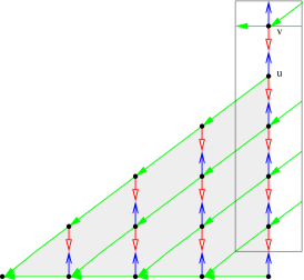
Figure 13.4: Example of a toroidal map where $d_{1}(u,z_{1}(u))$ has size $\Omega(n\times f)$.

Lemma 66

Let $u,v$ be vertices of $G^{\infty}$ such that $R_{i}(u)\subseteq R_{i}(v)$, then $u_{i}\leq v_{i}$. Moreover if $R_{i}(u)\subsetneq R_{i}(v)$, then $v_{i}-u_{i}>(N-n)(|R(L_{i-1}(u),L_{i-1}(v))|+|R(L_{i+1}(u),L_{i+1}(v))|)\geq 0$.

Proof.  We distinguish two cases depending of the fact that the Schnyder wood is of type 2.i or not.

$\bullet$ Case 1: The Schnyder wood is not of type 2.i.

Suppose first that $u$ and $v$ are both in a region delimited by two consecutive lines of color $i-1$ and two consecutive lines of color $i+1$. Let $L_{i-1}^{j},L_{i-1}^{j+1}$, $L_{i+1}^{j^{\prime}},L_{i+1}^{j^{\prime}+1}$ be these lines such that $L_{i-1}^{j+1}$ is on the positive side of $L_{i-1}^{j}$, $L_{i+1}^{j^{\prime}+1}$ is on the positive side of $L_{i+1}^{j^{\prime}}$, and $L_{k}^{\ell}\in\mathcal{L}_{k}^{\ell}$ (see Figure 13.5). We distinguish cases corresponding to equality or not between lines $L_{i-1}(u)$, $L_{i-1}(v)$ and $L_{i+1}(u)$, $L_{i+1}(v)$.

Figure 13.5: Position of $u$ and $v$ in the proof of Lemma 66

$\star$ Case 1.1: $L_{i-1}(u)=L_{i-1}(v)$ and $L_{i+1}(u)=L_{i+1}(v)$. Then $v_{i}-u_{i}=d_{i}(v,z_{i}(v))-d_{i}(u,z_{i}(u))=d_{i}(v,u)$. Thus clearly, if $R_{i}(u)\subseteq R_{i}(v)$, then $u_{i}\leq v_{i}$ and if $R_{i}(u)\subsetneq R_{i}(v)$, $v_{i}-u_{i}>0=(N-n)(|R(L_{i-1}(u),L_{i-1}(v))|+|R(L_{i+1}(u),L_{i+1}(v))|)$.

$\star$ Case 1.2: $L_{i-1}(u)=L_{i-1}(v)$ and $L_{i+1}(u)\neq L_{i+1}(v)$. As $u\in R_{i}(v)$, we have $L_{i+1}(u)=L_{i+1}^{j^{\prime}}$ and $L_{i+1}(v)=L_{i+1}^{j^{\prime}+1}$. Then $v_{i}-u_{i}=d_{i}(v,z_{i}(v))-d_{i}(u,z_{i}(u))+N(f_{i+1}(L_{i+1}(v))-f_{i+1}(L_{i+1}(u)))=d_{i}(v,z_{i}(v))-d_{i}(u,z_{i}(u))+Nf_{i+1}^{j^{\prime}}$. Let $u^{\prime}$ be the intersection of $P_{i+1}(u)$ with $L_{i-1}^{j+1}$ (maybe $u=u^{\prime}$). Let $v^{\prime}$ be the intersection of $P_{i+1}(v)$ with $L_{i-1}^{j+1}$ (maybe $v=v^{\prime}$). Since $L_{i+1}(u)\neq L_{i+1}(v)$, we have $u^{\prime}\neq v^{\prime}$. Since $u\in R_{i}(v)$, we have $u^{\prime}\in R_{i}(v^{\prime})$ and so $u^{\prime}\in P_{i-1}(v^{\prime})$. Then, by Lemma 65, $d_{i}(z_{i}(v^{\prime}),v^{\prime})+d_{i}(u^{\prime},z_{i}(u^{\prime}))<(n-1)f_{i+1}^{j^{\prime}}$. If $L_{i-1}(u)=L_{i-1}^{j+1}$ then, one can see that $d_{i}(v,z_{i}(v))-d_{i}(u,z_{i}(u))\geq d_{i}(v^{\prime},z_{i}(v^{\prime}))-d_{i}(u^{\prime},z_{i}(u^{\prime}))$. If $L_{i-1}(u)=L_{i-1}^{j}$, one can see that $d_{i}(v,z_{i}(v))-d_{i}(u,z_{i}(u))\geq d_{i}(v^{\prime},z_{i}(v^{\prime}))-d_{i}(u^{\prime},z_{i}(u^{\prime}))-f_{i+1}^{j^{\prime}}$. So finally, $v_{i}-u_{i}=d_{i}(v,z_{i}(v))-d_{i}(u,z_{i}(u))+Nf_{i+1}^{j^{\prime}}\geq d_{i}(v^{\prime},z_{i}(v^{\prime}))-d_{i}(u^{\prime},z_{i}(u^{\prime}))+(N-1)f_{i+1}^{j^{\prime}}>(N-n)f_{i+1}^{j^{\prime}}=(N-n)(|R(L_{i-1}(u),L_{i-1}(v))|+|R(L_{i+1}(u),L_{i+1}(v))|)\geq 0$.

$\star$ Case 1.3: $L_{i-1}(u)\neq L_{i-1}(v)$ and $L_{i+1}(u)=L_{i+1}(v)$. This case is completely symmetric to the previous case.

$\star$ Case 1.4: $L_{i-1}(u)\neq L_{i-1}(v)$ and $L_{i+1}(u)\neq L_{i+1}(v)$. As $u\in R_{i}(v)$, we have $L_{i+1}(u)=L_{i+1}^{j^{\prime}}$, $L_{i+1}(v)=L_{i+1}^{j^{\prime}+1}$, $L_{i-1}(u)=L_{i-1}^{j+1}$, and $L_{i-1}(v)=L_{i-1}^{j}$. Then $v_{i}-u_{i}=d_{i}(v,z_{i}(v))-d_{i}(u,z_{i}(u))+N(f_{i+1}(L_{i+1}(v))-f_{i+1}(L_{i+1}(u)))-N(f_{i-1}(L_{i-1}(v))-f_{i-1}(L_{i-1}(u)))=d_{i}(v,z_{i}(v))-d_{i}(u,z_{i}(u))+Nf_{i+1}^{j^{\prime}}+Nf_{i-1}^{j}$. Let $u^{\prime}$ be the intersection of $P_{i+1}(u)$ with $L_{i-1}^{j+1}$ (maybe $u=u^{\prime}$). Let $u^{\prime\prime}$ be the intersection of $P_{i-1}(u)$ with $L_{i+1}^{j^{\prime}}$ (maybe $u=u^{\prime\prime}$). Let $v^{\prime}$ be the intersection of $P_{i+1}(v)$ with $L_{i-1}^{j+1}$ (maybe $v=v^{\prime}$). Let $v^{\prime\prime}$ be the intersection of $P_{i-1}(v)$ with $L_{i+1}^{j^{\prime}}$ (maybe $v=v^{\prime\prime}$). Since $L_{i+1}(u)\neq L_{i+1}(v)$, we have $u^{\prime}\neq v^{\prime}$. Since $u\in R_{i}(v)$, we have $u^{\prime}\in R_{i}(v^{\prime})$ and so $u^{\prime}\in P_{i-1}(v^{\prime})$. Then, by Lemma 65, $d_{i}(z_{i}(v^{\prime}),v^{\prime})+d_{i}(u^{\prime},z_{i}(u^{\prime}))<(n-1)f_{i+1}^{j^{\prime}}$. Symmetrically, $d_{i}(z_{i}(v^{\prime\prime}),v^{\prime\prime})+d_{i}(u^{\prime\prime},z_{i}(u^{\prime\prime}))<(n-1)f_{i-1}^{j}$. Moreover, we have $d_{i}(v,z_{i}(v))-d_{i}(u,z_{i}(u))\geq d_{i}(v^{\prime},z_{i}(v^{\prime}))-d_{i}(u^{\prime},z_{i}(u^{\prime}))+d_{i}(v^{\prime\prime},z_{i}(v^{\prime\prime}))-d_{i}(u^{\prime\prime},z_{i}(u^{\prime\prime}))-f_{i+1}^{j^{\prime}}-f_{i-1}^{j}$. So finally, $v_{i}-u_{i}=d_{i}(v,z_{i}(v))-d_{i}(u,z_{i}(u))+Nf_{i+1}^{j^{\prime}}+Nf_{i-1}^{j}\geq d_{i}(v^{\prime},z_{i}(v^{\prime}))-d_{i}(u^{\prime},z_{i}(u^{\prime}))+d_{i}(v^{\prime\prime},z_{i}(v^{\prime\prime}))-d_{i}(u^{\prime\prime},z_{i}(u^{\prime\prime}))+(N-1)f_{i+1}^{j^{\prime}}+(N-1)f_{i-1}^{j}>(N-n)f_{i+1}^{j^{\prime}}+(N-n)f_{i-1}^{j}=(N-n)(|R(L_{i-1}(u),L_{i-1}(v))|+|R(L_{i+1}(u),L_{i+1}(v))|)\geq 0$.

Suppose now that $u$ and $v$ do not lie in a region delimited by two consecutive lines of color $i-1$ and/or in a region delimited by two consecutive lines of color $i+1$. One can easily find distinct vertices $w_{0},\ldots,w_{r}$ ($w_{i}$, $1\leq i<r$ chosen at intersections of monochromatic lines of colors $i-1$ and $i+1$) such that $w_{0}=u$, $w_{r}=v$, and for $0\leq\ell\leq r-1$, we have $R_{i}(w_{\ell})\subsetneq R_{i}(w_{\ell+1})$ and $w_{\ell},w_{\ell+1}$ are both in a region delimited by two consecutive lines of color $i-1$ and in a region delimited by two consecutive lines of color $i+1$. Thus by the first part of the proof, $(w_{\ell})_{i}-(w_{\ell+1})_{i}>(N-n)(|R(L_{i-1}(w_{\ell+1}),L_{i-1}(w_{\ell}))|+|R(L_{i+1}(w_{\ell+1}),L_{i+1}(w_{\ell}))|)$. Thus $v_{i}-u_{i}>(N-n)\sum_{\ell}(|R(L_{i-1}(w_{\ell+1}),L_{i-1}(w_{\ell}))|+|R(L_{i+1}(w_{\ell+1}),L_{i+1}(w_{\ell}))|)$. For any $a,b,c$ such $R_{i}(a)\subseteq R_{i}(b)\subseteq R_{i}(c)$, we have $|R(L_{j}(a),L_{j}(b))|+|R(L_{j}(b),L_{j}(c))|=|R(L_{j}(a),L_{j}(c))|$. Thus we obtain the result by summing the size of the regions.

$\bullet$ Case 2: The Schnyder wood is of type 2.i.

Suppose first that $u$ and $v$ are both in a region delimited by two consecutive lines of color $i+1$.

Let $L_{i+1}^{j},L_{i+1}^{j+1}$ be these lines such that $L_{i+1}^{j+1}$ is on the positive side of $L_{i+1}^{j}$, and $L_{i+1}^{\ell}\in\mathcal{L}_{i+1}^{\ell}$. We can assume that we do not have both $u$ and $v$ in $L_{i+1}^{j+1}$ (by eventually choosing other consecutive lines of color $i+1$). We consider two cases:

$\star$ Case 2.1: $v\notin L_{i+1}^{j+1}$. Then by Lemma 59, $L_{i+1}^{j}=L_{i+1}(u)=(L_{i-1}(u))^{-1}=L_{i+1}(v)=(L_{i-1}(v))^{-1}$. Then $v_{i}-u_{i}=d_{i}(v,z_{i}(v))-d_{i}(u,z_{i}(u))=d_{i}(v,u)$. Thus clearly, if $R_{i}(u)\subseteq R_{i}(v)$, then $u_{i}\leq v_{i}$ and if $R_{i}(u)\subsetneq R_{i}(v)$, then $v_{i}-u_{i}>0=(N-n)(|R(L_{i-1}(u),L_{i-1}(v))|+|R(L_{i+1}(u),L_{i+1}(v))|)$.

$\star$ Case 2.2: $v\in L_{i+1}^{j+1}$. Then $L_{i+1}^{j+1}=L_{i+1}(v)=(L_{i-1}(v))^{-1}$ and $d_{i}(v,z_{i}(v))=0$. By assumption $u\notin L_{i+1}^{j+1}$ and by Lemma 59, $L_{i+1}^{j}=L_{i+1}(u)=(L_{i-1}(u))^{-1}$. Then $v_{i}-u_{i}=d_{i}(v,z_{i}(v))-d_{i}(u,z_{i}(u))+N(f_{i+1}(L_{i+1}(v))-f_{i+1}(L_{i+1}(u)))-N(f_{i-1}(L_{i-1}(v))-f_{i-1}(L_{i-1}(u)))=-d_{i}(u,z_{i}(u))+2Nf_{i+1}^{j}$. Let $L_{i}$ and $L^{\prime}_{i}$ be two consecutive $i$-lines such that $u$ lies in the region between them and $L^{\prime}_{i}$ is on the right of $L_{i}$. Let $u^{\prime}$ be the intersection of $P_{i+1}(u)$ with $L_{i}$ (maybe $u=u^{\prime}$). Let $u^{\prime\prime}$ be the intersection of $P_{i-1}(u)$ with $L^{\prime}_{i}$ (maybe $u=u^{\prime\prime}$). Then, by Lemma 65, $d_{i}(u^{\prime},z_{i}(u^{\prime}))<(n-1)f_{i+1}^{j}$ and $d_{i}(u^{\prime\prime},z_{i}(u^{\prime\prime}))<(n-1)f_{i+1}^{j}$. Thus we have $d_{i}(u,z_{i}(u))\leq d_{i}(u^{\prime},z_{i}(u^{\prime}))+d_{i}(u^{\prime\prime},z_{i}(u^{\prime\prime}))+f_{i+1}^{j}<(2(n-1)+1)f_{i+1}^{j}$. So finally, $v_{i}-u_{i}>-(2n-1)f_{i+1}^{j}+2Nf_{i+1}^{j}>2(N-n)f_{i+1}^{j}=(N-n)(|R(L_{i-1}(u),L_{i-1}(v))|+|R(L_{i+1}(u),L_{i+1}(v))|)\geq 0$.

If $u$ and $v$ do not lie in a region delimited by two consecutive lines of color $i+1$, then as in case 1, one can find intermediate vertices to obtain the result. $\Box$

Lemma 67

If two vertices $u,v$ are adjacent, then for each color $i$, we have $|v_{i}-u_{i}|\leq 2Nf$.

Proof.  Since $u,v$ are adjacent, they are both in a region delimited by two consecutive lines of color $i-1$ and in a region delimited by two consecutive lines of color $i+1$. Let $L_{i-1}^{j},L_{i-1}^{j+1}$ be these two consecutive lines of color $i-1$ and $L_{i+1}^{j^{\prime}},L_{i+1}^{j^{\prime}+1}$ these two consecutive lines of color $i+1$ with $L_{k}^{\ell}\in\mathcal{L}_{k}^{\ell}$, $L_{i-1}^{j+1}$ is on the positive side of $L_{i-1}^{j}$ and $L_{i+1}^{j^{\prime}+1}$ is on the positive side of $L_{i+1}^{j^{\prime}}$ (see Figure 13.5 when the Schnyder wood is not of type 2.i). If the Schnyder wood is of type 2.i we assume that $L_{i-1}^{j+1}=(L_{i+1}^{j^{\prime}})^{-1}$ and $L_{i-1}^{j}=(L_{i+1}^{j^{\prime}+1})^{-1}$. Let $z$ be a vertex on the intersection of $L_{i-1}^{j+1}$ and $L_{i+1}^{j^{\prime}}$. Let $z^{\prime}$ be a vertex on the intersection of $L_{i-1}^{j}$ and $L_{i+1}^{j^{\prime}+1}$. Thus we have $R_{i}(z)\subseteq R_{i}(u)\subseteq R_{i}(z^{\prime})$ and $R_{i}(z)\subseteq R_{i}(v)\subseteq R_{i}(z^{\prime})$. So by Lemma 66, $z_{i}\leq u_{i}\leq z^{\prime}_{i}$ and $z_{i}\leq v_{i}\leq z^{\prime}_{i}$. So $|v_{i}-u_{i}|\leq z^{\prime}_{i}-z_{i}=N(f_{i+1}(L_{i+1}^{j^{\prime}+1})-f_{i+1}(L_{i+1}^{j^{\prime}})-N(f_{i-1}(L_{i-1}^{j})-f_{i-1}(L_{i-1}^{j+1}))=Nf_{i+1}^{j^{\prime}}+Nf_{i-1}^{j}\leq 2Nf$. $\Box$

We are now able to prove the following:

Theorem 24

If $G$ is a toroidal map given with an intersecting Schnyder wood, then the mapping of each vertex of $G^{\infty}$ on its region vector gives a geodesic embedding of $G$.

Proof.  By Lemmas 61 and 64, the mapping of $G^{\infty}$ on its region vector is periodic with respect to $S$, $S^{\prime}$ that are not collinear. For any pair $u,v$ of distinct vertices of $G^{\infty}$, by Lemma 32.(iii), there exists $i,j$ with $R_{i}(u)\subsetneq R_{i}(v)$ and $R_{j}(v)\subsetneq R_{j}(u)$ thus, by Lemma 66, $u_{i}<v_{i}$ and $v_{j}<u_{j}$. So $\mathcal{V}^{\infty}$ is a set of pairwise incomparable elements of $\mathbb{R}^{3}$.

(D1) $\mathcal{V}^{\infty}$ is a set of pairwise incomparable elements so the mapping between vertices of $G^{\infty}$ and $\mathcal{V}^{\infty}$ is a bijection.

(D2) Let $e=uv$ be an edge of $G^{\infty}$. We show that $w=u\vee v$ is on the surface $S_{\mathcal{V}^{\infty}}$. By definition $u\vee v$ is in $\mathcal{D}_{\mathcal{V}^{\infty}}$. Suppose, by contradiction that $w\notin S_{\mathcal{V}^{\infty}}$. Then there exist $x\in\mathcal{V}^{\infty}$ with $x<w$. Let $x$ also denote the corresponding vertex of $G^{\infty}$. Edge $e$ is in a region $R_{i}(x)$ for some $i$. So $u,v\in R_{i}(x)$ and thus by Lemma 32.(i), $R_{i}(u)\subseteq R_{i}(x)$ and $R_{i}(v)\subseteq R_{i}(x)$. Then by Lemma 66, $w_{i}=\max(u_{i},v_{i})\leq x_{i}$, a contradiction. Thus the elbow geodesic between $u$ and $v$ is on the surface.

(D3) Consider a vertex $v\in\mathcal{V}$ and a color $i$. Let $u$ be the extremity of the arc $e_{i}(v)$. We have $u\in R_{i-1}(v)$ and $u\in R_{i+1}(v)$, so by Lemma 32.(i), $R_{i-1}(u)\subseteq R_{i-1}(v)$ and $R_{i+1}(u)\subseteq R_{i+1}(v)$. Thus by Lemma 32.(iii), $R_{i}(v)\subsetneq R_{i}(u)$. So, by Lemma 66, $v_{i}<u_{i}$, $u_{i-1}\leq v_{i-1}$ and $u_{i+1}\leq v_{i+1}$. So the orthogonal arc of vertex $v$ in direction of the basis vector $e_{i}$ is part of the elbow geodesic of the edge $e_{i}(v)$.

(D4) Suppose there exists a pair of crossing edges $e=uv$ and $e^{\prime}=u^{\prime}v^{\prime}$ on the surface $S_{\mathcal{V}^{\infty}}$. The two edges $e,e^{\prime}$ cannot intersect on orthogonal arcs so they intersects on a plane orthogonal to one of the coordinate axis. Up to symmetry we may assume that we are in the situation of Figure 13.6 with $u_{1}=u^{\prime}_{1}$, $u_{2}>u^{\prime}_{2}$ and $v_{2}<v^{\prime}_{2}$. Between $u$ and $u^{\prime}$, there is a path consisting of orthogonal arcs only. With (D3), this implies that there is a bidirected path $P^{*}$ colored $0$ from $u$ to $u^{\prime}$ and colored $2$ from $u^{\prime}$ to $u$. We have $u\in R_{2}(v)$, so by Lemma 32.(i), $R_{2}(u)\subseteq R_{2}(v)$. We have $u^{\prime}\in R_{2}(u)$, so $u^{\prime}\in R_{2}(v)$. If $P_{0}(v)$ contains $u^{\prime}$, then there is a directed cycle containing $v,u,u^{\prime}$ in $G^{\infty}_{1}\cup(G^{\infty}_{0})^{-1}\cup(G^{\infty}_{2})^{-1}$, contradicting Lemma 6, so $P_{0}(v)$ does not contain $u^{\prime}$. If $P_{1}(v)$ contains $u^{\prime}$, then $u^{\prime}\in P_{1}(u)\cap P_{0}(u)$, contradicting Lemma 7. So $u^{\prime}\in R_{2}^{\circ}(v)$. Thus the edge $u^{\prime}v^{\prime}$ implies that $v^{\prime}\in R_{2}(v)$. So by Lemma 66, $v^{\prime}_{2}\leq v_{2}$, a contradiction. $\Box$

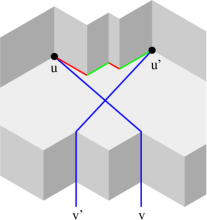
Figure 13.6: A pair of crossing elbow geodesic

Theorem 17 and 24 imply Theorem 23.

One can ask what is the “size” of the obtained geodesic embedding of Theorem 24? Of course this mapping is infinite so there is no real size, but as the object is periodic one can consider the smallest size of the vectors such that the mapping is periodic with respect to them. There are several such pairs of vectors, one is $S,S^{\prime}$. Recall that $S_{i}=N(c_{i+1}-c_{i-1})f$ and $S^{\prime}_{i}=N(c^{\prime}_{i+1}-c^{\prime}_{i-1})f$. Unfortunately the size of $S,S^{\prime}$ can be arbitrarily large. Indeed, the values of $c_{i+1}-c_{i-1}$ and $c^{\prime}_{i+1}-c^{\prime}_{i-1}$ are unbounded as a toroidal map can be artificially “very twisted” in the considered parallelogram representation (independently from the number of vertices or faces). Nevertheless we can prove existence of bounded size vectors for which the mapping is periodic with respect to them.

Lemma 68

If $G$ is a toroidal map given with an intersecting Schnyder wood, then the mapping of each vertex of $G^{\infty}$ on its region vector gives a periodic mapping of $G^{\infty}$ with respect to non collinear vectors $Y$ and $Y^{\prime}$ where the size of $Y$ and $Y^{\prime}$ is in $\mathcal{O}(\omega Nf)$. In general we have $\omega\leq n$ and in the case where $G$ is a simple toroidal triangulation given with a Schnyder wood obtained by Theorem 16, we have $\omega=1$.

Proof.  By Lemma 62, the vectors $Z_{i-1},Z_{i+1}$ (when the Schnyder wood is not of type 2.i) span a subset of $S,S^{\prime}$ (it can happen that this subset is strict). Thus in the parallelogram delimited by the vectors $Z_{i-1},Z_{i+1}$ (that is a parallelogram by Lemma 63), there is a parallelogram with sides $Y,Y^{\prime}$ containing a copy of $V$. The size of the vectors $Z_{i}$ is in $\mathcal{O}(\omega Nf)$ and so $Y$ and $Y^{\prime}$ also.

In general we have $\omega_{i}\leq n$ as each intersection between two monochromatic cycles of $G$ of color $i-1$ and $i+1$ corresponds to a different vertex of $G$ and thus $\omega\leq n$. In the case of simple toroidal triangulation given with a Schnyder wood obtained by Theorem 16, we have, for each color $i$, $\omega_{i}=1$, and thus $\omega=1$. $\Box$

Note that the geodesic embeddings of Theorem 24 are not necessarily rigid. A geodesic embedding is rigid [26, 41] if for every pair $u,v\in\mathcal{V}$ such that $u\vee v$ is in $\mathcal{S}_{\mathcal{V}}$, then $u$ and $v$ are the only elements of $\mathcal{V}$ that are dominated by $u\vee v$. The geodesic embedding of Figure 13.1 is not rigid has the bend corresponding to the loop of color $1$ is dominated by three vertices of $G^{\infty}$. We do not know if it is possible to build a rigid geodesic embedding from an intersecting Schnyder wood of a toroidal map. Maybe a technique similar to the one presented in [26] can be generalized to the torus.

It has been already mentioned that in the geodesic embeddings of Theorem 24 the points corresponding to vertices are not coplanar. The problem to build a coplanar geodesic embedding from the Schnyder wood of a toroidal map is open. In the plane, there are some examples of maps $G$ [26] for which it is no possible to require both rigidity and co-planarity. It is not difficult to transform these examples into toroidal maps such that the same is true is the toroidal case.

Another question related to co-planarity is whether one can require that the points of the orthogonal surface corresponding to edges of the graph (i.e. bends) are coplanar. This property is related to contact representation by homologous triangles [26]. It is known that in the plane, not all Schnyder woods are supported by such surfaces. Kratochvil’s conjecture [38], proved in [34], states that every 4-connected planar triangulation admits a contact representation by homothetic triangles. Can this be extended to the torus?

13.4 Example of a geodesic embedding

We use the example of the toroidal map $G$ of Figure 3.12 to illustrate the region vector method. This toroidal map has $n=3$ vertices, $f=4$ faces and $e=7$ edges. Let $N=n=3$. There are two edges that are oriented in two directions. The Schnyder wood is of type 1, with two $1$-cycles. We choose as origin the three bold monochromatic lines of Figure 13.7. We give them value $0$ and compute the other values $f_{i}(L)$ as explained in Section 13.2, i.e. we compute the “number” of faces between $L$ and the origin $L^{*}$ and put a minus if we are on the left of $L^{*}$ (this corresponds to values indicated on the border of Figure 13.7, that are values $0,-4,-8,-12$ for lines of color $0$, values $-4,-2,0,2,4$ for lines of color $1$ and values $0,4$ for lines of color $2$). Then we compute the region vector of the points according to Definition 9. For example, the point $v$ of Figure 13.7 as the following values (the three points $z_{i}(v)$ are represented on the figure): $v_{0}\ =\ d_{0}(v,z_{0}(v))\ +\ N\times\big{(}f_{1}(L_{1}(v))-f_{2}(L_{2}(v))\big{)}=0+3(0-0)=0$, $v_{1}\ =\ d_{1}(v,z_{1}(v))\ +\ N\times\big{(}f_{2}(L_{2}(v))-f_{0}(L_{0}(v))\big{)}=0+3(0-(-4))=12$, $v_{2}\ =\ d_{2}(v,z_{2}(v))\ +\ N\times\big{(}f_{0}(L_{0}(v))-f_{1}(L_{1}(v))\big{)}=1+3(-4-0)=-11$. We compute similarly the region vectors of all the vertices that are in the black box representing one copy of the graph and let $\mathcal{V}=\{(0,0,0),(0,12,-11),(6,12,-18)\}$ be the set of these vectors. Then we compute the $c_{i}$’s and $c^{\prime}_{i}$’s by algebraically counting the number of times the monochromatic cycles crosses the sides of the black box. A monochromatic cycle of color $0$ goes $-1$ time from right to left and $-2$ times from bottom to top. So $c_{0}=-1$ and $c^{\prime}_{0}=-2$. Similarly $c_{1}=0$, $c^{\prime}_{1}=1$, $c_{2}=1$, $c^{\prime}_{2}=0$. Then we compute $S_{i}=N(c_{i+1}-c_{i-1})f$ and $S^{\prime}_{i}=N(c^{\prime}_{i+1}-c^{\prime}_{i-1})f$ and obtain $S=(-12,24,-12)$, $S^{\prime}=(12,24,-36)$. Then the region vectors of the vertices of $G^{\infty}$ are $\{u\in\mathbb{R}^{3}\,|\,\exists\,v\in\mathcal{V},\ k_{1},k_{2}\in\mathbb{Z}$ such that $u=v+kS+k^{\prime}S\}$. In this example, the points are not coplanar, they lie on the two different planes of equation $x+y+z=0$ and $x+y+z=1$. The geodesic embedding that is obtained by mapping each vertex to its region vector is the geodesic embedding of Figure 13.1. The black parallelogram has sides the vectors $S,S^{\prime}$ and represent a basic tile.

Figure 13.7: Computation of the region vectors for the Schnyder wood of Figure 3.12.

13.5 Geodesic embedding and duality

Given an orthogonal surface generated by $\mathcal{V}$, let $\mathcal{F}_{\mathcal{V}}$ be the maximal points of $\mathcal{S}_{\mathcal{V}}$, i.e. the points of $\mathcal{S}_{\mathcal{V}}$ that are not dominated by any vertex of $\mathcal{S}_{\mathcal{V}}$. If $A,B\in\mathcal{F}_{\mathcal{V}}$ and $A\wedge B\in\mathcal{S}_{\mathcal{V}}$, then $\mathcal{S}_{\mathcal{V}}$ contains the union of the two line segments joining $A$ and $B$ to $A\wedge B$. Such arcs are called dual elbow geodesic. The dual orthogonal arc of $A\in\mathcal{F}_{\mathcal{V}}$ in the direction of the standard basis vector $e_{i}$ is the intersection of the ray $A+\lambda e_{i}$ with $\mathcal{S}_{\mathcal{V}}$.

Given a toroidal map $G$, let $G^{\infty*}$ be the dual of $G^{\infty}$. A dual geodesic embedding of $G$ is a drawing of $G^{\infty*}$ on the orthogonal surface $\mathcal{S}_{\mathcal{V}^{\infty}}$, where $\mathcal{V}^{\infty}$ is a periodic mapping of $G^{\infty}$ with respect to two non collinear vectors, satisfying the following (see example of Figure 13.8):

• There is a bijection between the vertices of $G^{\infty*}$ and $\mathcal{F}_{\mathcal{V}^{\infty}}$.

• Every edge of $G^{\infty*}$ is a dual elbow geodesic.

• Every dual orthogonal arc in $\mathcal{S}_{\mathcal{V}^{\infty}}$ is part of an edge of $G^{\infty*}$.

• There are no crossing edges in the embedding of $G^{\infty*}$ on $\mathcal{S}_{\mathcal{V}^{\infty}}$.

Figure 13.8: Dual geodesic embedding of the toroidal map of Figure 3.12.

Let $G$ be a toroidal map given with a intersecting Schnyder wood. Consider the mapping of each vertex on its region vector. We consider the dual of the Schnyder wood of $G$. By Proposition 10, it is an intersecting Schnyder wood of $G^{*}$. A face $F$ of $G^{\infty}$ is mapped on the point $\bigvee_{v\in F}v$. Let $\overline{G^{\infty}}$ be a simultaneous drawing of $G^{\infty}$ and $G^{\infty*}$ such that only dual edges intersect. To avoid confusion, we note $R_{i}$ the regions of the primal Schnyder wood and $R_{i}^{*}$ the regions of the dual Schnyder wood.

Lemma 69

For any face $F$ of $G^{\infty}$, we have that $\bigvee_{v\in F}v$ is a maximal point of $\mathcal{S}_{\mathcal{V}^{\infty}}$.

Proof.  Let $F$ be a face of $G^{\infty}$. For any vertex $u$ of $\mathcal{V}^{\infty}$, there exists a color $i$, such that the face $F$ is in the region $R_{i}(u)$. Thus for $v\in F$, we have $v\in R_{i}(u)$. By Lemma 66, we have $v_{i}\leq u_{i}$ and so $F_{i}\leq u_{i}$. So $F=\bigvee_{v\in F}v$ is a point of $\mathcal{S}_{\mathcal{V}^{\infty}}$.

Suppose, by contradiction, that $F$ is not a maximal point of $\mathcal{S}_{\mathcal{V}^{\infty}}$. Then there is a point $\alpha\in\mathcal{S}_{\mathcal{V}^{\infty}}$ that dominates $F$ and for at least one coordinate $j$, we have $F_{j}<\alpha_{j}$. Consider the angle labeling corresponding to the considered Schnyder wood. Every face is of type $1$ so the angles at $F$ form, in counterclockwise order, nonempty intervals of $0$’s, $1$’s, and $2$’s. For each color, let $z^{i}$ be a vertex of $F$ with angle $i$. We have $F$ is in the region $R_{i}(z^{i})$. So $z^{i-1}\in R_{i}(z^{i})$ and by Lemma 32.(i), we have $R_{i}(z^{i-1})\subseteq R_{i}(z^{i})$. Since $F$ is in $R_{i-1}(z^{i-1})$, it is not in $R_{i}(z^{i-1})$ and thus $R_{i}(z^{i-1})\subsetneq R_{i}(z^{i})$. Then by Lemma 66, we have $(z^{i-1})_{i}<(z^{i})_{i}$ and symmetrically $(z^{i+1})_{i}<(z^{i})_{i}$. So $F_{j-1}=(z^{j-1})_{j-1}>(z^{j})_{j-1}$ and $F_{j+1}>(z^{j})_{j+1}$. Thus $\alpha$ strictly dominates $z^{j}$, a contradiction to $\alpha\in\mathcal{S}_{\mathcal{V}^{\infty}}$. Thus $F$ is a maximal point of $\mathcal{S}_{\mathcal{V}^{\infty}}$ $\Box$

Lemma 70

If two faces $A,B$ are such that $R_{i}^{*}(B)\subseteq R_{i}^{*}(A)$, then $A_{i}\leq B_{i}$.

Proof.  Consider the angle labeling corresponding to the considered Schnyder wood. Let $v\in B$ be a vertex whose angle at $B$ is labeled $i$. We have $v\in R^{*}_{i}(B)$ and so $v\in R^{*}_{i}(A)$. In $\overline{G^{\infty}}$, the path $P_{i}(v)$ cannot leave $R^{*}_{i}(A)$, the path $P_{i+1}(v)$ cannot intersect $P_{i+1}(A)$ and the path $P_{i-1}(v)$ cannot intersect $P_{i-1}(A)$. Thus $P_{i+1}(v)$ intersect $P_{i-1}(A)$ and the path $P_{i-1}(v)$ intersect $P_{i+1}(A)$. So $A\in R_{i}(v)$. Thus for all $u\in A$, we have $u\in R_{i}(v)$, so $R_{i}(u)\subseteq R_{i}(v)$, and so $u_{i}\leq v_{i}$. Then $A_{i}=\max_{u\in A}u_{i}\leq v_{i}\leq\max_{w\in B}w_{i}=B_{i}$. $\Box$

Theorem 25

If $G$ is a toroidal map given with an intersecting Schnyder wood and each vertex of $G^{\infty}$ is mapped on its region vector, then the mapping of each face of $G^{\infty*}$ on the point $\bigvee_{v\in F}v$ gives a dual geodesic embedding of $G$.

Proof.  By Lemmas 61 and 64, the mapping is periodic with respect to non collinear vectors.

(D1*) Consider a counting of elements on the orthogonal surface, where we count two copies of the same object just once (note that we are on an infinite and periodic object). We have that the sum of primal orthogonal arcs plus dual ones is exactly $3m$. There are $3n$ primal orthogonal arcs and thus there are $3m-3n=3f$ dual orthogonal arcs. Each maximal point of $\mathcal{S}_{\mathcal{V}^{\infty}}$ is incident to $3$ dual orthogonal arcs and there is no dual orthogonal arc incident to two distinct maximal points. So there is $f$ maximal points. Thus by Lemma 69, we have a bijection between faces of $G^{\infty}$ and maximal points of $\mathcal{S}_{\mathcal{V}^{\infty}}$.

Let $\mathcal{V}^{\infty*}$ be the maximal points of $\mathcal{S}_{\mathcal{V}^{\infty}}$. Let $\mathcal{D}^{*}_{\mathcal{V}^{\infty}}=\{A\in\mathbb{R}^{3}\ |\ \exists\,B\in\mathcal{V}^{\infty*}$ such that $A\leq B\}$. Note that the boundary of $\mathcal{D}^{*}_{\mathcal{V}^{\infty}}$ is $\mathcal{S}_{\mathcal{V}^{\infty}}$.

(D2*) Let $e=AB$ be an edge of $G^{\infty*}$. We show that $w=A\wedge B$ is on the surface $S_{\mathcal{V}^{\infty}}$. By definition $w$ is in $\mathcal{D}^{*}_{\mathcal{V}^{\infty}}$. Suppose, by contradiction that $w\notin S_{\mathcal{V}^{\infty}}$. Then there exist $C$ a maximal point of $S_{\mathcal{V}^{\infty}}$ with $w<C$. By the bijection (D1*) between maximal point and vertices of $G^{\infty*}$, the point $C$ corresponds to a vertex of $G^{\infty*}$, also denoted $C$. Edge $e$ is in a region $R_{i}^{*}(C)$ for some $i$. So $A,B\in R_{i}^{*}(C)$ and thus, by Lemma 32.(i), $R_{i}^{*}(A)\subseteq R_{i}^{*}(C)$ and $R_{i}^{*}(B)\subseteq R_{i}^{*}(C)$. Then by Lemma 70, we have $C_{i}\leq\min(A_{i},B_{i})=w_{i}$, a contradiction. Thus the dual elbow geodesic between $A$ and $B$ is also on the surface.

(D3*) Consider a vertex $A$ of $G^{\infty*}$ and a color $i$. Let $B$ be the extremity of the arc $e_{i}(A)$. We have $B\in R_{i-1}^{*}(A)$ and $B\in R_{i+1}^{*}(A)$, so by Lemma 32.(i), $R_{i-1}^{*}(B)\subseteq R_{i-1}^{*}(A)$ and $R_{i+1}^{*}(B)\subseteq R_{i+1}^{*}(A)$. So by Lemma 70, $A_{i-1}\leq B_{i-1}$ and $A_{i+1}\leq B_{i+1}$. As $A$ and $B$ are distinct maximal point of $\mathcal{S}_{\mathcal{V}^{\infty}}$, they are incomparable, thus $B_{i}<A_{i}$. So the dual orthogonal arc of vertex $A$ in direction of the basis vector $e_{i}$ is part of edge $e_{i}(A)$.

(D4*) Suppose there exists a pair of crossing edges $e=AB$ and $e^{\prime}=A^{\prime}B^{\prime}$ of $G^{\infty*}$ on the surface $S_{\mathcal{V}^{\infty}}$. The two edges $e,e^{\prime}$ cannot intersect on orthogonal arcs so they intersects on a plane orthogonal to one of the coordinate axis. Up to symmetry we may assume that we are in the situation $A_{1}=A^{\prime}_{1}$, $A^{\prime}_{0}>A_{0}$ and $B^{\prime}_{0}<B_{0}$. Between $A$ and $A^{\prime}$, there is a path consisting of orthogonal arcs only. With (D3*), this implies that there is a bidirected path $P^{*}$ colored $2$ from $A$ to $A^{\prime}$ and colored $0$ from $A^{\prime}$ to $A$. We have $A\in R_{0}(B)$, so by Lemma 32.(i), $R_{0}(A)\subseteq R_{0}(B)$. We have $A^{\prime}\in R_{0}(A)$, so $A^{\prime}\in R_{0}(B)$. If $P_{2}(B)$ contains $A^{\prime}$, then there is a cycle containing $A,A^{\prime},B$ in $(G^{\infty}_{1})^{*}\cup(G^{\infty}_{0})^{*-1}\cup(G^{\infty}_{2})^{*-1}$, contradicting Lemma 6, so $P_{2}(B)$ does not contain $A^{\prime}$. If $P_{1}(B)$ contains $A^{\prime}$, then $A^{\prime}\in P_{1}(A)\cap P_{2}(A)$, contradicting Lemma 7. So $A^{\prime}\in R_{0}^{\circ}(B)$. Thus the edge $A^{\prime}B^{\prime}$ implies that $B^{\prime}\in R_{0}(B)$. So by Lemma 70, $B^{\prime}_{0}\geq B_{0}$, a contradiction. $\Box$

Theorems 24 and 25 can be combined to obtain a simultaneous representation of a Schnyder wood and its dual on an orthogonal surface. The projection of this 3-dimensional object on the plane of equation $x+y+z=0$ gives a representation of the primal and the dual where edges are allowed to have one bend and two dual edges have to cross on their bends (see example of Figure 13.9).

Theorem 26

An essentially 3-connected toroidal map admits a simultaneous flat torus representation of the primal and the dual where edges are allowed to have one bend and two dual edges have to cross on their bends. Such a representation is contained in a (triangular) grid of size $\mathcal{O}(n^{2}f)\times\mathcal{O}(n^{2}f)$ in general and $\mathcal{O}(nf)\times\mathcal{O}(nf)$ if the map is a simple triangulation. Furthermore the length of the edges are in $\mathcal{O}(nf)$.

Proof.  Let $G$ be an essentially 3-connected toroidal map. By Theorems 17 (or Theorem 16 if $G$ is a simple triangulation), $G$ admits an intersecting Schnyder wood (where monochromatic cycles of different colors intersect just once if $G$ is simple). By Theorems 24 and 25, the mapping of each vertex of $G^{\infty}$ on its region vector gives a primal and dual geodesic embedding. Thus the projection of this embedding on the plane of equation $x+y+z=0$ gives a representation of the primal and the dual of $G^{\infty}$ where edges are allowed to have one bend and two dual edges have to cross on their bends.

By Lemma 68, the obtained mapping is a periodic mapping of $G^{\infty}$ with respect to non collinear vectors $Y$ and $Y^{\prime}$ where the size of $Y$ and $Y^{\prime}$ is in $\mathcal{O}(\omega Nf)$, with $\omega\leq n$ in general and $\omega=1$ in case of a simple triangulation. Let $N=n$. The embedding gives a representation in a parallelogram of sides $Y,Y^{\prime}$ where the size of the vectors $Y$ and $Y^{\prime}$ is in $\mathcal{O}(n^{2}f)$ in general and in $\mathcal{O}(nf)$ if the graph is simple and the Schnyder wood is obtained by Theorem 16. By Lemma 67 the length of the edges in this representation are in $\mathcal{O}(nf)$. $\Box$

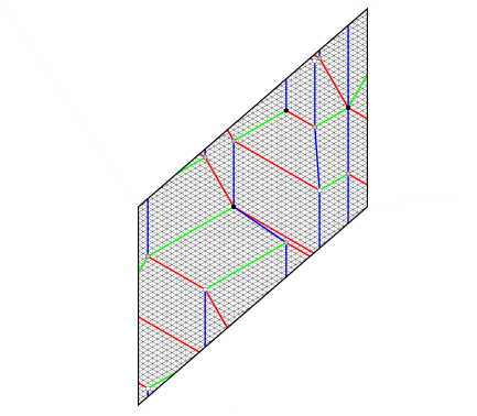
Figure 13.9: Simultaneous representation of the primal and the dual of the toroidal map of Figure 3.12 (see also Figure 7.5) with edges having one bend (in gray).

13.6 Straight-line representation

A straight-line representation of a toroidal map $G$ is the restriction to a parallelogram of a periodic straight-line representation of $G^{\infty}$. In the embeddings obtained by Theorem 23, vertices are not coplanar but we prove that for toroidal triangulations one can project the vertices on a plane to obtain a periodic straight-line representation of $G^{\infty}$ (see Figure 13.10).

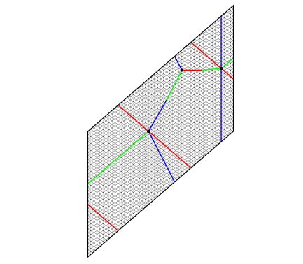
Figure 13.10: Straight-line representation of the map of Figure 3.12 obtained by projecting the geodesic embedding of Figure 13.1

For this purpose, we have to choose $N$ bigger than previously. Note that Figure 13.10 is the projection of the geodesic embedding of Figure 13.1 obtained with the value of $N=n$. In this particular case this gives a straight-line representation but in this section we only prove that such a technique works for triangulations and for $N$ sufficiently large. To obtain a straight-line representation of a general toroidal map, one first has to triangulate it.

Let $G$ be a toroidal triangulation given with an intersecting Schnyder wood and $V^{\infty}$ the set of region vectors of vertices of $G^{\infty}$. The Schnyder wood is crossing by Proposition 9. Recall that $\omega_{i}$ is the integer such that two monochromatic cycles of $G$ of colors $i-1$ and $i+1$ intersect exactly $\omega_{i}$ times.

Lemma 71

For any vertex $v$, the number of faces in the bounded region delimited by the three lines $L_{i}(v)$, for $i\in\{0,1,2\}$, is strictly less than $(5\min_{i}(\omega_{i})+\max_{i}(\omega_{i}))f$.

Proof.  Suppose by symmetry that $\min(\omega_{i})=\omega_{1}$. Let $L_{i}=L_{i}(v)$ and $z_{i}=z_{i}(v)$. Let $T$ be the bounded region delimited by the three monochromatic lines $L_{i}$. If $T$ is non empty, then its boundary is a cycle $C$ oriented clockwise or counterclockwise. Assume that $C$ is oriented counterclockwise (the proof is similar if oriented clockwise). The region $T$ is on the left sides of the lines $L_{i}$. We have $z_{i-1}\in P_{i}(z_{i+1})$.

We define, for $j,k\in\mathbb{N}$, monochromatic lines $L_{2}(j)$, $L_{0}(k)$ and vertices $z(j,k)$ as follows (see Figure 13.11). Let $L_{2}(1)$ be the first $2$-line intersecting $L_{0}\setminus\{z_{1}\}$ while walking from $z_{1}$, along $L_{0}$ in the direction of $L_{0}$. Let $L_{0}(1)$ be the first $0$-line of color $0$ intersecting $L_{2}\setminus\{z_{1}\}$ while walking from $z_{1}$, along $L_{2}$ in the reverse direction of $L_{2}$. Let $z(1,1)$ be the intersection between $L_{2}(1)$ and $L_{0}(1)$. Let $z(j,1)$, $j\geq 0$, be the consecutive copies of $z(1,1)$ along $L_{0}(1)$ such that $z(j+1,1)$ is after $z(j,1)$ in the direction of $L_{0}(1)$. Let $L_{2}(j)$, $j\geq 0$, be the $2$-line of color $2$ containing $z(j,1)$. Note that we may have $L_{2}=L_{2}(0)$ but in any case $L_{2}$ is between $L_{2}(0)$ and $L_{2}(1)$. Let $z(j,k)$, $k\geq 0$, be the consecutive copies of $z(j,1)$ along $L_{2}(j)$ such that $z(j,k+1)$ is after $z(j,k)$ in the reverse direction of $L_{2}(j)$. Let $L_{0}(k)$, $k\geq 0$, be the $0$-line containing $z(1,k)$. Note that we may have $L_{0}=L_{0}(0)$ but in any case $L_{0}$ is between $L_{0}(0)$ and $L_{0}(1)$. Let $S(j,k)$ be the region delimited by $L_{2}(j),L_{2}(j+1),L_{0}(k),L_{0}(k+1)$. All the region $S(j,k)$ are copies of $S(0,0)$. The region $S(0,0)$ may contain several copies of a face of $G$ but the number of copies of a face in $S(0,0)$ is equal to $\omega_{1}$. Let $R$ be the unbounded region situated on the right of $L_{0}(1)$ and on the right of $L_{2}(1)$. As $P_{0}(v)$ cannot intersect $L_{0}(1)$ and $P_{2}(v)$ cannot intersect $L_{2}(1)$, vertex $v$ is in $R$. Let $P(j,k)$ be the subpath of $L_{0}(k)$ between $z(j,k)$ and $z(j+1,k)$. All the lines $L_{0}(k)$ are composed only of copies of $P(0,0)$. The interior vertices of the path $P(0,0)$ cannot contains two copies of the same vertex, otherwise there will be a vertex $z(j,k)$ between $z(0,0)$ and $z(1,0)$. Thus all interior vertices of a path $P(j,k)$ corresponds to distinct vertices of $G$.

The Schnyder wood is crossing, thus $1$-lines are crossing $0$-lines. As a line $L_{0}(k)$ is composed only of copies of $P(0,0)$, any path $P(j,k)$ is crossed by a $1$-line. Let $L^{\prime}_{1}$ be the first $1$-line crossing $P(1,1)$ on a vertex $x$ while walking from $z(1,1)$ along $L_{0}(1)$. By the Schnyder property, line $L^{\prime}_{1}$ is not intersecting $R\setminus\{z(1,1)\}$. As $v\in R$ we have $L_{1}$ is on the left of $L^{\prime}_{1}$ (maybe $L_{1}=L^{\prime}_{1}$). Thus the region $T$ is included in the region $T^{\prime}$ delimited by $L_{0},L^{\prime}_{1},L_{2}$.

Let $y$ be the vertex where $L^{\prime}_{1}$ is leaving $S(1,1)$. We claim that $y\in L_{2}(1)$. Note that by the Schnyder property, we have $y\in L_{2}(1)\cup P(1,2)$. Suppose by contradiction that $y$ is an interior vertex of $P(1,2)$. Let $d_{x}$ be the length of the subpath of $P(1,1)$ between $z(1,1)$ and $x$. Let $d_{y}$ be the length of the subpath of $P(1,2)$ between $z(1,2)$ and $y$. Suppose $d_{y}<d_{x}$, then there should be a distinct copy of $L^{\prime}_{1}$ intersecting $P(1,1)$ between $z(1,1)$ and $x$ on a copy of $y$, a contradiction to the choice of $L^{\prime}_{1}$. So $d_{x}\leq d_{y}$. Let $A$ be the subpath of $L^{\prime}_{1}$ between $x$ and $y$. Let $B$ be the subpath of $P(1,1)$ between $x$ and the copy of $y$ (if $d_{x}=d_{y}$, then $B$ is just a single vertex). Consider all the copies of $A$ and $B$ between lines $L_{2}(1)$ and $L_{2}(2)$, they form an infinite line $L$ situated on the right of $L_{2}(1)$ that prevents $L^{\prime}_{1}$ from crossing $L_{2}(1)$, a contradiction.

By the position of $x$ and $y$. We have $L^{\prime}_{1}$ intersects $S(0,1)$ and $S(1,0)$. We claim that $L^{\prime}_{1}$ cannot intersect both $S(0,3)$ and $S(3,0)$. Suppose by contradiction that $L^{\prime}_{1}$ intersects both $S(0,3)$ and $S(3,0)$. Then $L^{\prime}_{1}$ is crossing $S(0,2)$ without crossing $L_{2}(0)$ or $L_{2}(1)$. Similarly $L^{\prime}_{1}$ is crossing $S(2,0)$ without crossing $L_{0}(0)$ or $L_{0}(1)$. Thus by superposing what happen in $S(0,2)$ and $S(2,0)$ in a square $S(j,k)$, we have that there are two crossing $1$-lines, a contradiction. Thus $L^{\prime}_{1}$ intersects at most one of $S(0,3)$ and $S(3,0)$.

Suppose that $L^{\prime}_{1}$ does not intersect $S(3,0)$. Then the part of $T^{\prime}$ situated right of $L_{0}(2)$ (left part on Figure 13.11) is strictly included in $(S(0,0)\cup S(1,0)\cup S(2,0)\cup S(0,1)\cup S(1,1))$. Thus this part of $T^{\prime}$ contains at most $5\omega_{1}f$ faces. Now consider the part of $T^{\prime}$ situated on the left of $L_{0}(2)$ (right part on Figure 13.11). Let $y^{\prime}$ be the intersection of $L^{\prime}_{1}$ with $L_{2}$. Let $Q$ be the subpath of $L^{\prime}_{1}$ between $y$ and $y^{\prime}$. By definition of $L_{2}(1)$, there are no $2$-lines between $L_{2}$ and $L_{2}(1)$. So $Q$ cannot intersect a $2$-line on one of its interior vertices. Thus $Q$ is crossing at most $\omega_{2}$ consecutive $0$-lines (that are not necessarily lines of type $L_{0}(k)$). Let $L^{\prime}_{0}$ be the $\omega_{2}+1$-th consecutive $0$-line that is on the left of $L_{0}(2)$ (counting $L_{0}(2)$). Then the part of $T^{\prime}$ situated on the left of $L_{0}(2)$ is strictly included in the region delimited by $L_{0}(2),L^{\prime}_{0},L_{2},L_{2}(1)$, and thus contains at most $\omega_{2}$ copies of a face of $G$. Thus $T^{\prime}$ contains at most $(\omega_{2}+5\omega_{1})f$ faces.

Symmetrically if $L^{\prime}_{1}$ does not intersect $S(0,3)$ we have that $T^{\prime}$ contains at most $(\omega_{0}+5\omega_{1})f$ faces. Then in any case, $T^{\prime}$ contains at most $(\max(\omega_{0},\omega_{2})+5\omega_{1})f$ faces and the lemma is true. $\Box$

Figure 13.11: Notations of the proof of Lemma 71.

The bound of Lemma 71 is somehow sharp. In the example of Figure 13.12, the rectangle represent a toroidal triangulation $G$ and the universal cover is partially represented. For each value of $k\geq 0$, there is a toroidal triangulation $G$ with $n=4(k+1)$ vertices, where the gray region, representing the region delimited by the three monochromatic lines $L_{i}(v)$ contains $4\sum_{j=1}^{2k+1}+3(2k+2)=\Omega(n\times f)$ faces. Figure 13.12 represent such a triangulation for $k=2$.

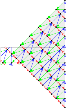
Figure 13.12: Example of a toroidal triangulation where the number of faces in the region delimited by the three monochromatic lines $L_{i}(v)$ contains $\Omega(n\times f)$ faces.

For planar maps the region vector method gives vertices that all lie on the same plane. This property is very helpful in proving that the position of the points on $P$ gives straight-line representations. In the torus, things are more complicated as our generalization of the region vector method does not give coplanar points. But Lemma 60 and 71 show that all the points lie in the region situated between the two planes of equation $x+y+z=0$ and $x+y+z=t$, with $t=(5\min(\omega_{i})+\max(\omega_{i}))f$. Note that $t$ is bounded by $6nf$ by Lemma 68 and this is independent from $N$. Thus from “far away” it looks like the points are coplanar and by taking $N$ sufficiently large, non coplanar points are “far enough” from each other to enable the region vector method to give straight-line representations.

Let $N=t+n$.

Lemma 72

Let $u,v$ be two vertices of $G^{\infty}$ such that $e_{i-1}(v)=uv$, $L_{i}=L_{i}(u)=L_{i}(v)$, and such that both $u$, $v$ are in the region $R(L_{i},L^{\prime}_{i})$ for $L^{\prime}_{i}$ a $i$-line consecutive to $L_{i}$. Then $v_{i+1}-u_{i+1}<|R(L_{i},L^{\prime}_{i})|$ and $e_{i-1}(v)$ is going counterclockwise around the closed disk bounded by $\{e_{i-1}(v)\}\cup P_{i}(u)\cup P_{i}(v)$.

Proof.  Let $y$ be the first vertex of $P_{i}(v)$ that is also in $P_{i}(u)$. Let $Q_{u}$ (resp. $Q_{v}$) the part of $P_{i}(u)$ (resp. $P_{i}(v)$) between $u$ (resp. $v$) and $y$.

Let $D$ be the closed disk bounded by the cycle $C=(Q_{v})^{-1}\cup\{e_{i-1}(v)\}\cup Q_{u}$. If $C$ is going clockwise around $D$, then $P_{i+1}(v)$ is leaving $v$ in $D$ and thus has to intersect $Q_{u}$ or $Q_{v}$. In both cases, there is a cycle in $G^{\infty}_{i+1}\cup(G^{\infty}_{i})^{-1}\cup(G^{\infty}_{i-1})^{-1}$, a contradiction to Lemma 6. So $C$ is going clockwise around $D$.

As $L_{i}(u)=L_{i}(v)$ and $L_{i-1}(u)=L_{i-1}(v)$, we have $v_{i+1}-u_{i+1}=d_{i+1}(v,u)$ and this is equal to the number of faces in $D$. We have $D\subsetneq R(L_{i},L^{\prime}_{i})$. Suppose $D$ contains two copies of a given face. Then, these two copies are on different sides of a $1$-line. By the Schnyder property, it is not possible to have a $1$-line entering $D$. So $D$ contains at most one copy of each face of $R(L_{i},L^{\prime}_{i})$. $\Box$

Lemma 73

For any face $F$ of $G^{\infty}$, incident to vertices $u,v,w$ (given in counterclockwise order around $F$), the cross product $\overrightarrow{vw}\wedge\overrightarrow{vu}$ has strictly positive coordinates.

Proof.  Consider the angle labeling corresponding to the Schnyder wood. The angles at $F$ are labeled in counterclockwise order $0,1,2$. As $\overrightarrow{uv}\wedge\overrightarrow{uw}=\overrightarrow{vw}\wedge\overrightarrow{vu}=\overrightarrow{wu}\wedge\overrightarrow{wv}$, we may assume that $u,v,w$ are such that $u$ is in the angle labeled $0$, vertex $v$ in the angle labeled $1$ and vertex $w$ in the angle labeled $2$. The face $F$ is either a cycle completely directed into one direction or it has two edges oriented in one direction and one edge oriented in the other. Let

$$\overrightarrow{X}=\overrightarrow{vw}\wedge\overrightarrow{vu}=\begin{pmatrix}(w_{1}-v_{1})(u_{2}-v_{2})-(w_{2}-v_{2})(u_{1}-v_{1})\\ -(w_{0}-v_{0})(u_{2}-v_{2})+(w_{2}-v_{2})(u_{0}-v_{0})\\ (w_{0}-v_{0})(u_{1}-v_{1})-(w_{1}-v_{1})(u_{0}-v_{0})\end{pmatrix}$$

By symmetry, we consider the following two cases:

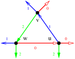
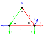
(a)		(b)

Figure 13.13: (a) case 1 and (b) case 2 of the proof of Lemma 73

$\bullet$ Case 1: the edges of the face $F$ are in counterclockwise order $e_{1}(u)$, $e_{2}(v)$, $e_{0}(w)$ (see Figure 13.13.(a)).

We have $v\in P_{1}(u)$, so $v\in R_{0}(u)\cap R_{2}(u)$ and $u\in R_{1}^{\circ}(v)$ (as there is no edges oriented in two direction). By Lemma 32, we have $R_{0}(v)\subseteq R_{0}(u)$ and $R_{2}(v)\subseteq R_{2}(u)$ and $R_{1}(u)\subsetneq R_{1}(v)$. In fact the first two inclusions are strict as $u\notin R_{0}(v)\cup R_{2}(v)$. So by Lemma 66, we have $v_{0}<u_{0}$, $v_{2}<u_{2}$, $u_{1}<v_{1}$. We can prove similar inequalities for the other pairs of vertices and we obtain $w_{0}<v_{0}<u_{0}$, $u_{1}<w_{1}<v_{1}$, $v_{2}<u_{2}<w_{2}$. By just studying the signs of the different terms occurring in the value of the coordinates of $\overrightarrow{X}$, it is clear that $\overrightarrow{X}$ as strictly positive coordinates. (For the first coordinates, it is easier if written in the following form $X_{0}=(u_{1}-w_{1})(v_{2}-w_{2})-(u_{2}-w_{2})(v_{1}-w_{1})$.)

$\bullet$ Case 2: the edges of the face $F$ are in counterclockwise order $e_{0}(v)$, $e_{2}(v)$, $e_{0}(w)$.(see Figure 13.13.(b)).

As in the previous case, one can easily obtain the following inequalities: $w_{0}<v_{0}<u_{0}$, $u_{1}<w_{1}<v_{1}$, $u_{2}<v_{2}<w_{2}$ (the only difference with case $1$ is between $u_{2}$ and $v_{2}$). Exactly like in the previous case, it is clear to see that $X_{0}$ and $X_{2}$ are strictly positive. But there is no way to reformulate $X_{1}$ to have a similar proof. Let $A=w_{2}-v_{2}$, $B=u_{0}-v_{0}$, $C=v_{0}-w_{0}$ and $D=v_{2}-u_{2}$, so $X_{1}=AB-CD$ and $A,B,C,D$ are all strictly positive.

Vertices $u,v,w$ are in the region $R(L_{1},L^{\prime}_{1})$ for $L^{\prime}_{1}$ a $1$-line consecutive to $L_{1}$. We consider two cases depending on equality or not between $L_{1}(u)$ and $L_{1}(v)$.

$\star$ Subcase 2.1: $L_{1}(u)=L_{1}(v)$.

We have $X_{1}=A(B-D)+D(A-C)$.

We have $B-D=(u_{0}+u_{2})-(v_{0}+v_{2})=(v_{1}-u_{1})+(\sum u_{i}-\sum v_{i})$. Since $u\in P_{0}(v)$, we have $L_{0}(u)=L_{0}(v)$. Suppose that $L_{2}(u)=L_{2}(v)$, then by Lemma 60, we have $\sum u_{i}=\sum v_{i}$, and thus $B-D=v_{1}-u_{1}>0$. Suppose now that $L_{2}(u)\neq L_{2}(v)$. By Lemmas 60 and 71, $\sum u_{i}-\sum v_{i}>-t$. By Lemma 66, $v_{1}-u_{1}>(N-n)|R(L_{2}(u),L_{2}(v))|\geq N-n$. So $B-D>N-n-t\geq 0$.

We have $A-C=(w_{0}+w_{2})-(v_{0}+v_{2})=(v_{1}-w_{1})+(\sum w_{i}-\sum v_{i})>\sum w_{i}-\sum v_{i}$. Suppose that $L_{1}(v)=L_{1}(w)$, then by Lemma 60, we have $\sum v_{i}=\sum w_{i}$ and thus $A-C=v_{1}-w_{1}>0$. Then $X_{1}>0$. Suppose now that $L_{1}(v)\neq L_{1}(w)$. By Lemma 72, $D=v_{2}-u_{2}<|R(L_{1},L^{\prime}_{1})|$. By Lemma 66, $A=w_{2}-v_{2}>(N-n)|R(L_{1},L^{\prime}_{1})|$. By Lemmas 60 and 71, $\sum w_{i}-\sum v_{i}>-t$, so $A-C>-t$. Then $X_{1}>(N-n-t)|R(L_{1},L^{\prime}_{1})|>0$.

$\star$ Subcase 2.2: $L_{1}(u)\neq L_{1}(v)$.

We have $X_{1}=B(A-C)+C(B-D)$.

Suppose that $L_{1}(w)\neq L_{1}(v)$. Then $L_{1}(w)=L_{1}(u)$. By Lemma 72, $e_{0}(w)$ is going counterclockwise around the closed disk $D$ bounded by $\{e_{0}(w)\}\cup P_{1}(w)\cup P_{1}(u)$. Then $v$ is inside $D$ and $P_{1}(v)$ has to intersect $P_{1}(w)\cup P_{1}(u)$, so $L_{1}(v)=L_{1}(u)$, contradicting our assumption. So $L_{1}(v)=L_{1}(w)$.

By Lemma 66, $B=u_{0}-v_{0}>(N-n)|R(L_{1},L^{\prime}_{1})|$. We have $A-C=(w_{0}+w_{2})-(v_{0}+v_{2})=(v_{1}-w_{1})+(\sum w_{i}-\sum v_{i})$. By Lemma 60, we have $\sum v_{i}=\sum w_{i}$ and thus $A-C=v_{1}-w_{1}>0$. By (the symmetric of) Lemma 72, $C=v_{0}-w_{0}<|R(L_{1},L^{\prime}_{1})|$. By Lemmas 60 and 71, $B-D=(u_{0}+u_{2})-(v_{0}+v_{2})=(v_{1}-u_{1})+(\sum u_{i}-\sum v_{i})>-t$. So $X_{1}>(N-n-t)|R(L_{1},L^{\prime}_{1})|>0$. $\Box$

Let $G$ be an essentially 3-connected toroidal map. Consider a periodic mapping of $G^{\infty}$ embedded graph $H$ (finite or infinite) and a face $F$ of $H$. Denote $(f_{1},f_{2},\ldots,f_{t})$ the counterclockwise facial walk around $F$. Given a mapping of the vertices of $H$ in $\mathbb{R}^{2}$, we say that $F$ is correctly oriented if for any triplet $1\leq i_{1}<i_{2}<i_{3}\leq t$, the points $f_{i_{1}}$, $f_{i_{2}}$, and $f_{i_{3}}$ form a counterclockwise triangle. Note that a correctly oriented face is drawn as a convex polygon.

Lemma 74

Let $G$ be an essentially 3-connected toroidal map given with a periodic mapping of $G^{\infty}$ such that every face of $G^{\infty}$ is correctly oriented. This mapping gives a straight-line representation of $G^{\infty}$.

Proof.  We proceed by induction on the number of vertices $n$ of $G$. Note that the theorem holds for $n=1$, so we assume that $n>1$. Given any vertex $v$ of $G$, let $(u_{0},u_{1},\ldots,u_{d-1})$ be the sequence of its neighbors in counterclockwise order (subscript understood modulo $d$). Every face being correctly oriented, for every $i\in[0,d-1]$ the oriented angle (oriented counterclockwise) $(\overrightarrow{vu_{i}},\overrightarrow{vu_{i+1}})<\pi$. Let the winding number $k_{v}$ of $v$ be the integer such that $2k_{v}\pi=\sum_{i\in[0,d-1]}(\overrightarrow{vu_{i}},\overrightarrow{vu_{i+1}})$. It is clear that $k_{v}\geq 1$. Let us prove that $k_{v}=1$ for every vertex $v$.

Claim 6

For any vertex $v$, its winding number $k_{v}=1$.

Proof.  In a parallelogram representation of $G$, we can sum up all the angles by grouping them around the vertices or around the faces.

$$\sum_{v\in V(G)}\sum_{u_{i}\in N(v)}(\overrightarrow{vu_{i}},\overrightarrow{vu_{i+1}})=\sum_{F\in F(G)}\sum_{f_{i}\in F}(\overrightarrow{f_{i}f_{i-1}},\overrightarrow{f_{i}f_{i+1}})$$

The face being correctly oriented, they form convex polygons. Thus the angles of a face $F$ sum at $(|F|-2)\pi$.

$$\sum_{v\in V(G)}2k_{v}\pi=\sum_{F\in F(G)}(|F|-2)\pi$$

$$\sum_{v\in V(G)}k_{v}=\frac{1}{2}\sum_{F\in F(G)}|F|-f$$

$$\sum_{v\in V(G)}k_{v}=m-f$$

So by Euler’s formula $\sum_{v\in V(G)}k_{v}=n$, and thus $k_{v}=1$ for every vertex $v$. $\Diamond$

Let $v$ be a vertex of $G$ that minimizes the number of loops whose ends are on $v$. Thus either $v$ has no incident loop, or every vertex is incident to at least one loop.

Assume that $v$ has no incident loop. Let $v^{\prime}$ be any copy of $v$ in $G^{\infty}$ and denote its neighbors $(u_{0},u_{1},\ldots,u_{d-1})$ in counterclockwise order. As $k_{v}=1$, the points $u_{0},u_{1},\ldots,u_{d-1}$ form a polygon $P$ containing the point $v^{\prime}$ and the segments $[v^{\prime},u_{i}]$ for any $i\in[0,d-1]$. It is well known that any polygon, admits a partition into triangles by adding some of the chords. Let us call $O$ the outerplanar graph with outer boundary $(u_{0},u_{1},\ldots,u_{d-1})$, obtained by this “triangulation” of $P$. Let us now consider the toroidal map $G^{\prime}=(G\setminus\{v\})\cup O$ and its periodic embedding obtained from the mapping of $G^{\infty}$ by removing the copies of $v$. It is easy to see that in this embedding every face of $G^{\prime}$ is correctly oriented (including the inner faces of $O$, or the faces of $G$ that have been shortened by an edge $u_{i}u_{i+1}$). Thus by induction hypothesis, the mapping gives a straight-line representation of $G^{\prime\infty}$. It is also a straight-line representation of $G^{\infty}$ minus the copies of $v$ where the interior of each copy of the polygons $P$ are pairwise disjoint and do not intersect any vertex or edge. Thus one can add the copies of $v$ on their initial positions and add the edges with their neighbors without intersecting any edge. The obtained drawing is thus a straight-line representation of $G^{\infty}$.

Assume now that every vertex is incident to at least one loop. Since these loops are non-contractible and do not cross each other, they form homothetic cycles. Thus $G$ is as depicted in Figure 13.14, where the dotted segments stand for edges that may be in $G$ but not necessarily. Since the mapping is periodic the edges corresponding to loops of $G$ form several parallel lines, cutting the plane into infinite strips. Since for any $1\leq i\leq n$, $k_{v_{i}}=1$, a line of copies of $v_{i}$ divides the plane, in such a way that their neighbors which are copies of $v_{i-1}$ and their neighbors which are copies of $v_{i+1}$ are in distinct half-planes. Thus adjacent copies of $v_{i}$ and $v_{i+1}$ are on two lines bounding a strip. Then one can see that the edges between copies of $v_{i}$ and $v_{i+1}$ are contained in this strip without intersecting each other. Thus the obtained mapping of $G^{\infty}$ is a straight-line representation. $\Box$

Figure 13.14: The graph $G$ if every vertex is incident to a loop.

A plane is positive if it has equation $\alpha x+\beta y+\gamma z=0$ with $\alpha,\beta,\gamma\geq 0$.

Theorem 27

If $G$ is a toroidal triangulation given with a crossing Schnyder wood, and $V^{\infty}$ the set of region vectors of vertices of $G^{\infty}$. Then the projection of $V^{\infty}$ on a positive plane gives a straight-line representation of $G^{\infty}$.

Proof.  Let $\alpha,\beta,\gamma\geq 0$ and consider the projection of $V^{\infty}$ on the plane $P$ of equation $\alpha x+\beta y+\gamma z=0$. A normal vector of the plane is given by the vector $\overrightarrow{n}=(\alpha,\beta,\gamma)$. Consider a face $F$ of $G^{\infty}$. Suppose that $F$ is incident to vertices $u,v,w$ (given in counterclockwise order around $F$). By Lemma 73, $(\overrightarrow{uv}\wedge\overrightarrow{uw}).\overrightarrow{n}$ is positive. Thus the projection of the face $F$ on $P$ is correctly oriented. So by Lemma 74, the projection of $V^{\infty}$ on $P$ gives a straight-line representation of $G^{\infty}$. $\Box$

Theorems 13 and 27 implies the following:

Theorem 28

A toroidal map admits a straight-line flat torus representation in a polynomial size grid.

Indeed, any toroidal map $G$ can be transformed into a toroidal triangulation $G^{\prime}$ by adding a linear number of vertices and edges and such that $G^{\prime}$ is simple if and only if $G$ is simple (see for example the proof of Lemma 2.3 of [42]). Then by Theorem 13, $G^{\prime}$ admits a crossing Schnyder wood. By Theorem 27, the projection of the set of region vectors of vertices of $G^{\prime\infty}$ on a positive plane gives a straight-line representation of $G^{\prime\infty}$. The grid where the representation is obtained can be the triangular grid, if the projection is done on the plane of equation $x+y+z=0$, or the square grid, if the projection is done on one of the plane of equation $x=0$, $y=0$ or $z=0$. By Lemma 68, and the choice of $N$, the obtained mapping is a periodic mapping of $G^{\infty}$ with respect to non collinear vectors $Y$ and $Y^{\prime}$ where the size of these vectors is in $\mathcal{O}(\omega^{2}n^{2})$ with $\omega\leq n$ in general and $\omega=1$ if the graph is simple and the Schnyder wood obtained by Theorem 16. By Lemma 67, the length of the edges in this representation are in $\mathcal{O}(n^{3})$ in general and in $\mathcal{O}(n^{2})$ if the graph is simple. When the graph is not simple, there is a non-contractible cycle of length $1$ or $2$ and thus the size of one of the two vectors $Y$, $Y^{\prime}$ is in $\mathcal{O}(n^{3})$. Thus the grid obtained in Theorem 28 has size in $\mathcal{O}(n^{3})\times\mathcal{O}(n^{4})$ in general and $\mathcal{O}(n^{2})\times\mathcal{O}(n^{2})$ if the graph is simple.

The method presented here gives a polynomial algorithm to obtain straight-line representation of any toroidal maps in polynomial size grids. Indeed, all the proofs leads to polynomial algorithms, even the proof of Theorem 15 [28] which uses results from Robertson and Seymour [47] on disjoint paths problems.

It would be nice to extend Theorem 27 to obtain convex straight-line representation for essentially 3-connected toroidal maps.

Note that the results presented in this chapter motivated Castelli Aleardi, Devillers and Fusy [15] to develop direct methods to obtain straight line representations for toroidal maps. They manage to generalize planar canonical ordering to the cylinder to obtain straight-line representation of toroidal triangulations in grids of size $\mathcal{O}(n)\times\mathcal{O}(n^{\frac{3}{2}})$.

Conclusion

In this manuscript we propose a generalization of Schnyder woods to higher genus oriented surfaces. For this purpose we keep the simplicity of the local definition of Schnyder woods in the plane and extend it to surfaces. A drawback is the loss of the main global property of the planar case : the partition into three trees (see Figures 1.6 and 2.3). Nevertheless in the toroidal case we are able to define some other global properties that a Schnyder wood may have or may not have (crossing, balanced, minimality, etc.) that enable to understand the structure of the manipulated objects and use it for nice applications like graph drawing or optimal encoding. Many questions were raised all along the manuscript concerning toroidal Schnyder woods, let us recall one of the simplest property that one may ask: does a simple toroidal triangulation admit a Schnyder wood where each of the three colors induces a connected subgraph? Among the numerous applications of planar Schnyder woods that are still to be generalized to the torus, we hope that the obtained bijection can be used to generate random toroidal triangulations with uniform distribution.

In the toroidal case ($g=1$), Euler’s formula ensures that every vertex plays exactly the same role. When going to higher genus ($g\geq 2$), some strange things happen with the need of special vertices satisfying “several times” the local property (see Figure 3.1). The lattice structure of homologous orientations is a general result that is valid in this context but we are not yet able to find a proof of existence of the considered objects. We only conjecture that, when $g\geq 2$, a map admits a Schnyder wood if and only if it is essentially 3-connected. Also we have no guess of what would be some global interesting property in this case. Indeed, generalizing the global properties that we found for the torus is not straightforward since one has to deal with the special vertices. For example the definition of $\gamma$ is not anymore “stable by homology”, i.e. if two non-contractible cycles $C,C^{\prime}$ are homologous, we may have $\gamma(C)\neq\gamma(C^{\prime})$ whereas we have equality on the torus by Lemma 33.

Originally Schnyder woods were defined for planar triangulations and then, by allowing edges to be oriented in two directions, they have been generalized to (internally) 3-connected planar maps. Thus this manuscript is written for the general situation of (essentially) 3-connected maps except when we prove results that are specific to triangulations. We may have adopted a different point of view where instead of generalizing toward 3-connected maps we would have generalized toward $d$-angulations.

Indeed, there are many kinds of planar maps that admit orientations that are similar to Schnyder woods. For example planar 4-connected triangulations admit so-called transversal structures [31], quadrangulations admit 2-orientations [5], $d$-angulations of girth $d$ admit $\frac{d}{d-2}$-orientations [8], even-degree maps admit Eulerian orientations [49], corner triangulations admits partition into $3$ bipolar orientations [20], etc. Among these different kind of orientations, Schnyder woods (for triangulations) and 2-orientations (for quadrangulations) can be seen has particular cases of $\frac{d}{d-2}$-orientations (for $d$-angulations of girth $d$). We do not see a common way to present these different orientations in a unified framework so we choose to present this manuscript on Schnyder woods only as this is certainly one of the most famous objects of this kind (and also the one that we started to look at).

Nevertheless it seems that several structural properties that have been presented in this manuscript for Schnyder woods in higher genus are still valid in the context of $\frac{d}{d-2}$-orientations. Figure 13.15 gives examples of toroidal $d$-angulations for $d=3,4,5,6$ given with $\frac{d}{d-2}$-orientations, i.e. assignments of positive integers, on the half-edges of the map $G$ such that, for every edge, the weights of its two half-edges sum to $d-2$, and for every vertex, the weights of its incident half-edges sum to $d$. Such a fractional orientation of $G$ can be seen as a classical orientation in the $(d-2)$-multigraph $H$ obtained from $G$ by replacing every edge by $d-2$ parallel edges. Indeed having a $\frac{d}{d-2}$-orientation of $G$ is equivalent of having an orientation of the edges of $H$ (in one direction only) where every vertex has outdegree exactly $d$. A notion (and existence !) of balanced orientation can then be defined similarly as in this manuscript. Then the lattice structure in the multigraph naturally define a minimal element that can be used for bijection purpose. A similar story can be told for transversal structures (see Figure 13.16) by looking at the angle graph to define the balanced property (and also maybe for other kind of orientations?) but we are at a point where this manuscript should stop and of course research continues …

$d=3$	$d=4$	$d=5$	$d=6$

Figure 13.15: Example of $\frac{d}{d-2}$-orientations of toroidal maps for $d=3,4,5,6$.

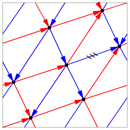
Figure 13.16: The minimal balanced transversal structure of $K_{7}$ w.r.t. to the rooted (dashed) edge.

Bibliography

- [1] B. Albar, D. Gonçalves, K. Knauer, Orienting triangulations, Journal of Graph Theory 83 (2016) 392-405.
- [2] M. Albenque, D. Poulalhon, Generic method for bijections between blossoming trees and planar maps, Electronic Journal of Combinatorics 22 (2015) P2.38.
- [3] J. Barát, C. Thomassen, Claw-decompositions and tutte-orientations, Journal of Graph Theory 52 (2006) 135-146.
- [4] J. Barbay, L. Castelli Aleardi, M. He, J. I. Munro, Succinct representation of labeled graphs, Algorithmica 61 (2012) 224-257.
- [5] L. Barrière, C. Huemer, 4-labelings and grid embeddings of plane quadrangulations, GD 2010, Lecture Notes in Computer Science 5849 (2010) 413-414.
- [6] O. Bernardi, Bijective counting of tree-rooted maps and shuffles of parenthesis systems, Electronic Journal of Combinatorics 14 (2007) R9.
- [7] O. Bernardi, G. Chapuy A bijection for covered maps, or a shortcut between Harer-Zagier’s and Jackson’s formulas, Journal of Combinatorial Theory A 118 (2011) 1718-1748.
- [8] O. Bernardi, E. Fusy, A bijection for triangulations, quadrangulations, pentagulations, etc., Journal of Combinatorial Theory A 119 (2012) 218-244.
- [9] N. Bonichon, C. Gavoille, N. Hanusse, An information-theoretic upper bound of planar graphs using triangulation, STACS 2003, Lecture Notes in Computer Science 2607 (2003) 499-510.
- [10] N. Bonichon, A bijection between realizers of maximal plane graphs and pairs of non-crossing dyck paths, Discrete Mathematics 298 (2005) 104-114.
- [11] N. Bonichon, S. Felsner, M. Mosbah, Convex drawings of 3-connected plane graphs, Algorithmica 47 (2007) 399-420.
- [12] N. Bonichon, C. Gavoille, N. Hanusse, D. Ilcinkas, Connections between theta-graphs, delaunay triangulations, and orthogonal surfaces, WG 2010, Lecture Notes in Computer Science 6410 (2010) 266-278.
- [13] L. Castelli Aleardi, E. Fusy, T. Lewiner, Schnyder woods for higher genus triangulated surfaces, with applications to encoding, Discrete and Computational Geometry 42 (2009) 489-516.
- [14] L. Castelli Aleardi, E. Fusy, T. Lewiner, Optimal encoding of triangular and quadrangular meshes with fixed topology, CCCG 2010.
- [15] L. Castelli Aleardi, O. Devillers, E. Fusy, Canonical ordering for triangulations on the cylinder, with applications to periodic straight-line drawings, GD 2012, Lecture Notes in Computer Science 7704 (2012) 376-387.
- [16] E. Chambers, D. Eppstein, M. Goodrich, M. Löffler, Drawing graphs in the plane with a prescribed outer face and polynomial area, GD 2010, Lecture Notes in Computer Science 6502 (2011) 129-140.
- [17] V. Despré, D. Gonçalves, B. Lévêque, Encoding toroidal triangulations, Discrete and Computational Geometry (2016) 1-38.
- [18] E. Duchi, D. Poulalhon, G. Schaeffer, Uniform random sampling of simple branched coverings of the sphere by itself, SODA 2014 294-304.
- [19] C. Duncan, M. Goodrich, S. Kobourov, Planar drawings of higher-genus graphs, Journal of Graph Algorithms and Applications 15 (2011) 13-32.
- [20] D. Eppstein, E. Mumford, Steinitz theorems for simple orthogonal polyhedra, Journal of Computational Geometry 5 (2014) 179-244.
- [21] S. Felsner, Convex drawings of planar graphs and the order dimension of 3-polytopes, Order 18 (2001) 19-37.
- [22] S. Felsner, Geodesic embeddings and planar graphs, Order 20 (2003) 135-150.
- [23] S. Felsner, Lattice structures from planar graphs, Electronic Journal of Combinatorics 11 (2004) R15.
- [24] S. Felsner, Geometric Graphs and Arrangements, Vieweg, 2004.
- [25] S. Felsner, W. T. Trotter, Posets and planar graphs, Journal Graph Theory 49 (2005) 273-284.
- [26] S. Felsner, F. Zickfeld, Schnyder woods and orthogonal surfaces, Discrete and Computational Geometry 40 (2008) 103-126.
- [27] S. Felsner, K. Knauer, ULD-lattices and -bonds, Combinatorics, Probability and Computing 18 (2009) 707-724.
- [28] G. Fijavz, personal communication, 2011.
- [29] H. de Fraysseix, P. Ossona de Mendez, P. Rosenstiehl, On triangle contact graphs, Combinatorics, Probability and Computing 3 (1994) 233-246.
- [30] H. de Fraysseix, P. Ossona de Mendez, On topological aspects of orientations, Discrete Mathematics 229 (2001) 57-72.
- [31] E. Fusy, Transversal structures on triangulations: a combinatorial study and straight-line drawings, Discrete Mathematics 309 (2009) 1870-1894.
- [32] P. Giblin, Graphs, surfaces and homology, Cambridge University Press, Cambridge, third edition, 2010.
- [33] D. Gonçalves, B. Lévêque, A. Pinlou, Triangle contact representations and duality, Discrete and Computational Geometry 48 (2012) 239-254.
- [34] D. Gonçalves, B. Lévêque, A. Pinlou, Triangle contact representations and duality, GD 2010, Lecture Notes in Computer Science 6502 (2011) 262-273.
- [35] D. Gonçalves, B. Lévêque, Toroidal maps: Schnyder woods, orthogonal surfaces and straight-line representations, Discrete and Computational Geometry 51 (2014) 67-131.
- [36] D. Gonçalves, K. Knauer, B. Lévêque, On the structure of Schnyder woods on orientable surfaces, manuscript, 2015. arXiv:1501.05475
- [37] G. Kant, Drawing planar graphs using the canonical ordering, Algorithmica 16 (1996) 4-32.
- [38] J. Kratochvíl, Bertinoro Workshop on Graph Drawing, 2007.
- [39] W. S. Massey, Algebraic Topology: An Introduction, Harcourt, Brace and World, New York, 1967
- [40] F. Meunier, personal communication, 2015.
- [41] E. Miller, Planar graphs as minimal resolutions of trivariate monomial ideals, Documenta Mathematica 7 (2002) 43-90.
- [42] B. Mohar, Straight-line representations of maps on the torus and other flat surfaces, Discrete Mathematics 155 (1996) 173-181.
- [43] B. Mohar, P. Rosenstiehl, Tessellation and visibility representations of maps on the torus, Discrete and Computational Geometry 19 (1998) 249-263.
- [44] P. Ossona de Mendez, Orientations bipolaires, PhD Thesis, manuscript, 1994.
- [45] D. Poulalhon, G. Schaeffer, Optimal coding and sampling of triangulations, Algorithmica 46 (2006) 505-527.
- [46] J. Propp, Lattice structure for orientations of graphs, manuscript, 1993. arXiv:math/0209005
- [47] N. Robertson, P.D Seymour, Graph minors. VI. Disjoint paths across a disc,Journal of Combinatorial Theory B 41 (1986) 115-138.
- [48] P. Rosenstiehl, Embedding in the plane with orientation constraints: The angle graph, Annals of New York Academy of Sciences 555 (1989) 340-346.
- [49] G. Schaeffer, Bijective census and random generation of eulerian planar maps with prescribed vertex degrees, Electronics Journal of Combinnatorics 4 (1997) R20.
- [50] W. Schnyder, Planar graphs and poset dimension, Order 5 (1989) 323-343.
- [51] W. Schnyder, Embedding planar graphs on the grid, SODA 1990 138-148.
- [52] T. Ueckerdt, Geometric representations of graphs with low polygonal complexity, PhD thesis, manuscript, 2011.