Simple, Fast and Lightweight Parallel Wavelet Tree Construction

Abstract

The wavelet tree (Grossi et al. [SODA, 2003]) and wavelet matrix (Claude et al. [Inf. Syst., 47:15–32, 2015]) are compact indices for texts over an alphabet $[0,\sigma)$ that support rank, select and access queries in $O(\lg\sigma)$ time. We first present new practical sequential and parallel algorithms for wavelet tree construction. Their unifying characteristics is that they construct the wavelet tree bottom-up, i. e., they compute the last level first. We also show that this bottom-up construction can easily be adapted to wavelet matrices. In practice, our best sequential algorithm is up to twice as fast as the currently fastest sequential wavelet tree construction algorithm (Shun [DCC, 2015]), simultaneously saving a factor of 2 in space. This scales up to 32 cores, where we are about equally fast as the currently fastest parallel wavelet tree construction algorithm (Labeit et al. [DCC, 2016]), but still use only about 75 % of the space. An additional theoretical result shows how to adapt any wavelet tree construction algorithm to the wavelet matrix in the same (asymptotic) time, using only little extra space.

1 Introduction

The wavelet tree (WT), introduced in 2003 by Grossi et al. [10], is a space-efficient data structure that can answer access, rank, and select queries for a text over an alphabet $[0,\sigma)$ in $\mathop{}\mathopen{}\mathcal{O}\mathopen{}\left(\lg\sigma\right)$ time, requiring just ${n\lceil\lg\sigma\rceil(1+o(1))}$ bits of space. WTs are used as a basic data structure in many applications, e. g., text indexing [10], compression [16, 11], and in computational geometry as an alternative to fractional cascading [14]. More information on the history of wavelet trees and many more of their applications can be found in the survey articles by Ferragina et al. [5] and Navarro [18].

1.1 Our Contributions.

In this paper, we focus on the construction of wavelet trees, but the reader should note that with some trivial modifications all our sequential and parallel algorithms work as well for wavelet matrices (and are actually also implemented for both variants). The highlights of our new algorithms are the following:

• We present the fastest sequential WT-construction algorithms (pcWT and psWT) that are up to twice as fast as serialWT [20], the previously fastest implementation for wavelet trees.

• Simultaneously, our new algorithms use much less space than all previous ones: on realistically sized alphabets, pcWT uses almost no space in addition to the input and output, while psWT uses only one additional array of the same size as the text. Previous ones such as serialWT or recWT [13] use at least twice as much additional space.

• We parallelize our new algorithms, obtaining the fastest parallel WT-construction algorithms on medium-sized workstations of up to 32 cores.

• In particular, this results in the first practical parallel algorithms for wavelet matrices.

A final (theoretical) contribution of this paper is that we show that the wavelet tree and the wavelet matrix are equivalent, in the sense that every algorithm that can compute the former can also compute the latter in the same time with only $(n+\sigma)(1+o(1))+(\sigma+2)\lceil\lg n\rceil$ bits of additional space.

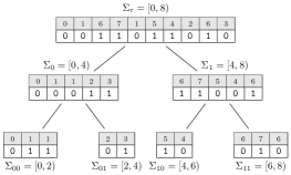
(a) Pointer-based wavelet tree.

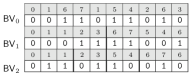
(b) Level-wise wavelet tree.

(c) Binary representation of $\mathop{}\mathopen{}\mathsf{T}\mathopen{}$.

Figure 1: The text $\mathop{}\mathopen{}\mathsf{T}\mathopen{}=\texttt{0167154263}$, its binary representation in LABEL:sub@sfig:example_text, and the the two variants of wavelet trees of $\mathop{}\mathopen{}\mathsf{T}\mathopen{}$. The light gray ( ) arrays contain the characters represented at the corresponding position in the bit vector and are not a part of the WT. In LABEL:sub@sfig:example_pWT, $\Sigma_{\alpha}$ denotes the characters that are represented by the bit vector for $\alpha\in\{r,0,1,00,01,10,11\}$. In LABEL:sub@sfig:example_lWT, thick lines represent the borders of the intervals.

1.2 Further Related Work.

There exists lots of theoretical work when it comes to WT-construction. One line of research addresses lowering the construction time below $\mathop{}\mathopen{}\mathcal{O}\mathopen{}\left(n\lg\sigma\right)$, which is possible on a word-RAM by using word packing techniques. Babenko et al. [1] and Munro et al. [17] independently obtained a construction time of $\mathop{}\mathopen{}\mathcal{O}\mathopen{}\left(n\lceil\lg\sigma/\sqrt{\lg n}\rceil\right)$. Recently, Shun [21] has parallelized the word packing approach by Babenko et al. [1] to improve the construction to $\mathop{}\mathopen{}\mathcal{O}\mathopen{}\left(\sigma+\lg n\right)$ parallel time requiring $\mathop{}\mathopen{}\mathcal{O}\mathopen{}\left(n\lceil\lg\sigma/\sqrt{\lg n}\rceil\right)$ work (here and in the following, we analyze parallel algorithms using JáJá’s work-time paradigm [12]).

Fuentes-Sepúlveda et al. [7] were the first to describe and implement practical parallel WT-construction algorithms, requiring $\mathop{}\mathopen{}\mathcal{O}\mathopen{}\left(n\right)$ time and $\mathop{}\mathopen{}\mathcal{O}\mathopen{}\left(n\lg\sigma\right)$ work. Faster practical approaches were presented subsequently by Shun [20] and by Labeit et al. [13], both requiring $\mathop{}\mathopen{}\mathcal{O}\mathopen{}\left(\lg n\lg\sigma\right)$ time and $\mathop{}\mathopen{}\mathcal{O}\mathopen{}\left(n\lg\sigma\right)$ work.

A different line of research addresses the (theoretical) working space during construction: Claude et al. [3] and Tischler [22] showed how to reduce the construction space for the WT to $O(\lg n)$ bits. However, none of these algorithms have been implemented beyond a proof-of-concept-status.

Although many papers (e. g., [20, 21]) on wavelet tree construction mention that their algorithms can also be adapted to wavelet matrices, none of them has actually been implemented. The only (sequential and semi-external) implementation of a WM-construction algorithm we are aware of is from the succinct data structure library (SDSL) [8]. Finally, we mention that a faster and smaller alternative to the WT (that can only be used in very specific text indexing applications) can be constructed semi-externally [9] and that there is a recent online WT-construction algorithm [4].

2 Preliminaries

Let $\mathsf{T}=\mathop{}\mathopen{}\mathsf{T}\mathopen{}[0]\dots\mathop{}\mathopen{}\mathsf{T}\mathopen{}[n-1]$ be a text of length $n$ over an alphabet $\Sigma=[0,\sigma)$. Each character $\mathop{}\mathopen{}\mathsf{T}\mathopen{}[i]$ can be represented using $\lceil\lg\sigma\rceil$ bits. In this paper, the leftmost bit is the most significant bit (MSB) and the least significant bit (LSB) is the rightmost bit. We denote the binary representation of a character $\alpha\in\Sigma$ as $\mathop{}\mathopen{}\mathop{\text{bits}}\mathopen{}\left(\alpha\right)$, e. g. $\mathop{}\mathopen{}\mathop{\text{bits}}\mathopen{}\left(3\right)=(\mathtt{011})_{2}$. Whenever we write a binary representation of a value, we indicate it by a subscript two. The $k$-th bit (from MSB to LSB) of a character $\alpha$ is denoted by $\mathop{}\mathopen{}\mathop{\text{bit}}\mathopen{}\left(k,\alpha\right)$ for all $0\leq k<\lceil\lg\sigma\rceil$. Given $\alpha\in\Sigma$, the bit prefix of size $k$ of $\alpha$ are the $k$ most significant bits, i. e., $\mathop{}\mathopen{}\mathop{\text{prefix}}\mathopen{}\left(k,\alpha\right)=(\mathop{}\mathopen{}\mathop{\text{bit}}\mathopen{}\left(0,\alpha\right)\dots\mathop{}\mathopen{}\mathop{\text{bit}}\mathopen{}\left(k-1,\alpha\right))_{2}$. We interpret sequences of bits as integer values.

Let $\mathsf{BV}$ be a bit vector of size $n$. The operation $\textnormal{{rank}}_{0}(\mathsf{BV},i)$ returns the number of 0’s in $\mathsf{BV}[0,i)$, whereas $\textnormal{{select}}_{0}(\mathsf{BV},i)$ returns the position of the $i$-th 0 in $\mathsf{BV}$. The operations $\textnormal{{rank}}_{1}(\mathsf{BV},i)$ and $\textnormal{{select}}_{1}(\mathsf{BV},i)$ are defined analogously.

Given an array A of $n$ integers and an associative operator $+$ (we only use addition), the zero based prefix sum for A returns an array $\textsf{B}[0,n)$ with $\textsf{B}[0]=0$ and $\textsf{B}[i]=\textsf{A}[i-1]+\textsf{B}[i-1]$ for all $i\in[1,n)$. The prefix sum can be computed in $\mathop{}\mathopen{}\mathcal{O}\mathopen{}\left(\lg n\right)$ parallel time and $\mathop{}\mathopen{}\mathcal{O}\mathopen{}\left(n\right)$ work [12].

Wavelet Trees.

Let $\mathop{}\mathopen{}\mathsf{T}\mathopen{}$ be a text of length $n$ over an alphabet $[0,\sigma)$. The wavelet tree (WT) of $\mathop{}\mathopen{}\mathsf{T}\mathopen{}$ is a complete and balanced binary tree. Each node of the WT represents characters in $[\ell,r)\subseteq[0,\sigma)$. The root of the WT represents characters in $[0,\sigma)$, i. e., all characters. The left (or right) child of a node representing characters in $[\ell,r)$ represents the characters in $[\ell,(\ell+r)/2)$ (or $[(\ell+r)/2,r)$, respectively). A node is a leaf if $l+2\geq r$.

The characters in $[\ell,r)$ at a node $v$ are represented using a bit vector $\mathsf{BV}_{v}$ such that the $i$-th bit in $\mathsf{BV}_{v}$ is $\mathop{}\mathopen{}\mathop{\text{bit}}\mathopen{}\left(d(v),{\mathop{}\mathopen{}\mathsf{T}\mathopen{}_{[\ell,r)}}[i]\right)$, where $d(v)$ is the depth of $v$ in WT, i. e., the number of edges on the path from the root to $v$, and $\mathop{}\mathopen{}\mathsf{T}\mathopen{}_{[\ell,r)}$ denotes the array containing the characters of $\mathop{}\mathopen{}\mathsf{T}\mathopen{}$ (in the same order) that are in $[\ell,r)$. The interval of a WT at which a character is represented at level $\ell$ is encoded by its length-$\ell$ bit prefix, as shown in the following Observation:

Observation 1 (Fuentes-Sepúlveda et al. [6]).

Given a character $\mathop{}\mathopen{}\mathsf{T}\mathopen{}[i]$ for $i\in[0,n)$ and a level $\ell\in[1,\lceil\lg\sigma\rceil)$ of the WT, the interval pertinent to $\mathop{}\mathopen{}\mathsf{T}\mathopen{}[i]$ in $\mathsf{BV}_{\ell}$ can be computed by $\mathop{}\mathopen{}\mathop{\text{prefix}}\mathopen{}\left(\ell,\mathop{}\mathopen{}\mathsf{T}\mathopen{}[i]\right)$.

There are two variants of the WT: the pointer-based and the level-wise WT. The pointer-based WT uses pointers to represent the tree structure, see Figure 1a. In the level-wise WT, we concatenate the bit vectors of all nodes at the same depth in a pointer-based WT. Since we lose the tree topology, the resulting bit vectors correspond to a level that is equal to the depth of the concatenated nodes. We store only a single bit vector $\mathsf{BV}_{\ell}$ for each level $\ell\in[0,\lceil\lg\sigma\rceil)$, see Figure 1b. This retains the functionality from the pointer-based WT [14, 15], but reduces the redundancy for the binary rank- and select-structures on the bit vectors.

The wavelet tree (both variants) can be used to generalize the operations access, rank and select from bit vectors to alphabets of size $\sigma$. Answering these queries then requires $\mathop{}\mathopen{}\mathcal{O}\mathopen{}\left(\lg\sigma\right)$ time. To do so, the bit vectors are augmented by binary rank and select structures. We point to [2] for a detailed description of the operations. In the following, we work with the level-wise WT.

3 New Wavelet Tree Construction Algorithms

As shown in Observation 1, each level $\ell$ of the WT contains disjoint intervals corresponding to the length-$\ell$ bit prefixes of the characters in $\mathop{}\mathopen{}\mathsf{T}\mathopen{}$. This enables us to start on the last level $\lceil\lg\sigma\rceil-1$, and then iteratively work through the other levels in a bottom-up manner until the tree is fully constructed. To get this process started, we need to know the borders of the intervals on the last level, for which we must first compute the histogram of the text characters (as in the first phase of counting sort). On subsequent levels $\ell\in[0,\lceil\lg\sigma\rceil-1)$ we use the fact that we can quickly compute the histograms of the considered bit prefixes of size $\ell$ from the histogram of bit prefixes of size $\ell+1$, without rescanning the text. Saving one scan of the text per level is one of the reasons that our algorithms are faster. This and the resulting low memory consumption (up to 50 % of the competitors) are the main distinguishing features of our new algorithms from the previous WT-construction algorithms. We assume that arrays are initialized with 0’s. In this section, $id$ refers to the identity function. Later (when we construct wavelet matrices in §5), we need to replace the identity function with the bit-reversal permutation.

3.1 Sequential Wavelet Tree Construction.

Our first WT-construction algorithm (pcWT, see Algorithm 1) starts with the computation of the number of occurrences of each character in $\mathop{}\mathopen{}\mathsf{T}\mathopen{}$ to fill the initial histogram $\textsf{Hist}[0,\sigma)$. In addition, the first level of the WT is computed, as it contains the MSBs of all characters in text order (lines 1 and 1). This requires $\mathop{}\mathopen{}\mathcal{O}\mathopen{}\left(n\right)$ time and $\sigma\lceil\lg n\rceil$ bits space for the histogram. Later on we require additional $\sigma\lceil\lg n\rceil$ bits to store the starting positions of the intervals (see array $\mathop{}\mathopen{}\mathsf{SPos}\mathopen{}[0,\sigma)$ in Algorithm 1).

Initially, we have a histogram for all characters in $\mathop{}\mathopen{}\mathsf{T}\mathopen{}$. During each iteration (say at level $\ell$) we need the histogram for all bit prefixes of size $\ell-1$ of the characters in $\mathop{}\mathopen{}\mathsf{T}\mathopen{}$. Therefore, if we have the histogram of length-$\ell$ bit prefixes, we can simply compute the histogram of the bit prefixes of size $\ell-1$ by ignoring the last bit of the current prefix. E. g., the amount of characters with bit prefix $(\mathtt{01})_{2}$ is the total number of characters with bit prefixes $(\mathtt{010})_{2}$ and $(\mathtt{011})_{2}$. We can do so in $\mathop{}\mathopen{}\mathcal{O}\mathopen{}\left(\sigma\right)$ time requiring no additional space reusing the space of the histogram of length-$\ell$ bit prefixes (line 1).

Using the updated histogram, we compute the starting positions of the intervals of the characters that can by identified by their bit prefix of size $\ell-1$ for level $\ell$. The starting position of the interval representing characters with bit prefix $0$ is always $0$, therefore we only compute the starting positions for all other bit prefixes (line 1). Again, this requires $\mathop{}\mathopen{}\mathcal{O}\mathopen{}\left(\sigma\right)$ time and no additional space, as we can reuse the space used to store the starting positions of the intervals of the previously considered level.

Last, we need to compute the bit vector for the current level $\ell$. To do so, we simply scan $\mathop{}\mathopen{}\mathsf{T}\mathopen{}$ once from left to right and consider the bit prefix of length $\ell-1$ of each character. Since we have computed the the starting position ($\mathop{}\mathopen{}\mathsf{SPos}\mathopen{}$) in the bit vector where the $\ell$-th MSB of the characters needs to be stored, we can store it accordingly and increase the position for characters with the same bit prefix by one (lines 1 and 1). This requires $\mathop{}\mathopen{}\mathcal{O}\mathopen{}\left(n\right)$ time and no additional space. Since we need to compute $\mathop{}\mathopen{}\mathcal{O}\mathopen{}\left(\lg\sigma\right)$ levels, this results in the following Lemma:

Lemma 1.

Algorithm pcWT computes the WT of a text of length $n$ over an alphabet of size $\sigma$ in $\mathop{}\mathopen{}\mathcal{O}\mathopen{}\left(n\lg\sigma\right)$ time using $2\sigma\lceil\lg n\rceil$ bits of space in addition to the input and output.

1 for $i=0$ to $n-1$ do

2       $\mathop{}\mathopen{}\mathsf{Hist}\mathopen{}[\mathop{}\mathopen{}\mathsf{T}\mathopen{}[i]]\textsf{++}$

3       $\mathsf{BV}_{0}[i]=\textnormal{{Bit}}(0,\mathop{}\mathopen{}\mathsf{T}\mathopen{}[i])$

4for $\ell=\lceil\lg\sigma\rceil-1$ to $1$ do

5       for $i=0$ to $2^{\ell}-1$ do

6             $\mathop{}\mathopen{}\mathsf{Hist}\mathopen{}[i]=\mathop{}\mathopen{}\mathsf{Hist}\mathopen{}[2i]+\mathop{}\mathopen{}\mathsf{Hist}\mathopen{}[2i+1]$

7      for $i=1$ to $2^{\ell}-1$ do

8             $\mathop{}\mathopen{}\mathsf{SPos}\mathopen{}[id(i)]=\mathop{}\mathopen{}\mathsf{SPos}\mathopen{}[id(i-1)]+\mathop{}\mathopen{}\mathsf{Hist}\mathopen{}[id(i-1)]$

9      for $i=0$ to $n-1$ do

10             $pos=\mathop{}\mathopen{}\mathsf{SPos}\mathopen{}[\mathop{}\mathopen{}\mathop{\text{prefix}}\mathopen{}\left(\ell,\mathop{}\mathopen{}\mathsf{T}\mathopen{}[i]\right)]\textsf{++}$

11             $\mathsf{BV}_{\ell}[pos]=\mathop{}\mathopen{}\mathop{\text{bit}}\mathopen{}\left(\ell,\mathop{}\mathopen{}\mathsf{T}\mathopen{}[i]\right)$

Algorithm 1 pcWT (sequential)

3.2 Parallel Wavelet Tree Construction.

The naïve way to parallelize the pcWT algorithm is to parallelize it such that each core is responsible for the construction of one level of the WT. To this end, each core needs to first compute the corresponding histogram of the level, and then the resulting starting positions of the intervals (each requiring $2^{\ell}\lceil\lg n\rceil$ bits of space at level $\ell$). This results in the following Lemma:

Lemma 2.

The parallelization of pcWT computes the WT in $\mathop{}\mathopen{}\mathcal{O}\mathopen{}\left(n\right)$ time with $\mathop{}\mathopen{}\mathcal{O}\mathopen{}\left(n\lg\sigma\right)$ work requiring $4\sigma\lceil\lg n\rceil$ bits of space in addition to the input and output.

The disadvantage of this naïve parallelization is that we cannot efficiently use more than $\lceil\lg\sigma\rceil$ cores. To use more cores, instead of parallelizing level-wise, we could do the following. Each of the $p$ cores gets a slice of the text of size $\Theta(\frac{n}{p})$ and computes the corresponding bits in the bit vectors on all levels. On level $\ell$, each core $c$ first computes its local histogram $\mathop{}\mathopen{}\mathsf{Hist}\mathopen{}_{c}[0,\sigma)$ according to the length-$\ell$ bit-prefixes of the input characters. Using a parallel zero based prefix sum operation, these local histograms are then combined such that in the end each core knows where to write its bits (arrays $\mathop{}\mathopen{}\mathsf{SPos}\mathopen{}_{c}[0,\sigma)$ for $c\in[0,p)$). As in the sequential algorithm, the final writing is then accomplished by scanning the local slice of the text from left to right, writing the bits to their correct places in $\mathsf{BV}_{\ell}$, and incrementing the corresponding value in $\mathop{}\mathopen{}\mathsf{SPos}\mathopen{}_{c}$.

This comes with the problem that two or more cores may want to concurrently write bits to the same computer word, resulting in race conditions. To avoid these race conditions, one would have to implement mechanisms for exclusive writes, which would result in unacceptably slow running times. We rather propose the following approaches.

3.2.1 Using Sorting.

Instead of having each core write randomly to each bit vector $\mathsf{BV}_{\ell}$, we want each core to be responsible for the same interval on each level of the WT. To this end, we globally sort the input text (using the starting positions $\mathop{}\mathopen{}\mathsf{SPos}\mathopen{}_{c}$ on level $\ell$). The resulting sorted text $\mathsf{T}_{\text{sorted}}$ is then again split into slices of size $\Theta(\frac{n}{p})$. Then, each core scans its local slice from left to right and writes the corresponding bits to the bit vector $\mathsf{BV}_{\ell}$ (also from left to right). To avoid race conditions and false sharing, i. e., working on data in a cache line that has been changed by another core, we further make sure that the size of each slice of the text is a common multiple of the cache lines’ length and the size of a computer word.

The resulting parallel WT-construction algorithm (psWT, see Algorithm 2) works as follows: First, each of the $p$ cores computes the local histogram ($\mathop{}\mathopen{}\mathsf{Hist}\mathopen{}_{c}$ for $c\in[0,p)$) of its slice of $\mathop{}\mathopen{}\mathsf{T}\mathopen{}$ and, at the same time, fills $\mathsf{BV}_{0}$ (lines 2 and 2). We compute the local starting positions ($\mathop{}\mathopen{}\mathsf{SPos}\mathopen{}_{c}$ for $c\in[0,p)$), using the zero based prefix sum of $\mathop{}\mathopen{}\mathsf{SPos}\mathopen{}_{0}[0],\mathop{}\mathopen{}\mathsf{SPos}\mathopen{}_{1}[0],\dots,\mathop{}\mathopen{}\mathsf{SPos}\mathopen{}_{p-1}[0],\dots,\mathop{}\mathopen{}\mathsf{SPos}\mathopen{}_{0}[\sigma-1],\dots,\mathop{}\mathopen{}\mathsf{SPos}\mathopen{}_{p-1}[\sigma-1]$, with respect to (w.r.t.) $id$, see line 2. Here, “w.r.t. $id$” means that character $id(i)$ follows character $id(i-1)$ for all $i\in[1,2^{j})$. Note that we replace $id$ with the bit-reversal permutation when constructing WMs in §5.1. All in all this requires $\mathop{}\mathopen{}\mathcal{O}\mathopen{}\left(\lg p+\sigma\right)$ time, $\mathop{}\mathopen{}\mathcal{O}\mathopen{}\left(n+p\sigma\right)$ work and $2p\sigma\lceil\lg n\rceil$ bits of space using $p$ cores. Using this information ($\mathop{}\mathopen{}\mathsf{Hist}\mathopen{}_{c}$ and $\mathop{}\mathopen{}\mathsf{SPos}\mathopen{}_{c}$), we can compute the corresponding values of $\mathop{}\mathopen{}\mathsf{Hist}\mathopen{}_{c}$ and $\mathop{}\mathopen{}\mathsf{SPos}\mathopen{}_{c}$ for all levels $\ell\in[1,\lceil\lg\sigma\rceil)$.

For each level (see loop starting at line 2) the time and work required are the same as during the first step. There is no additional space required since we can reuse the space used during the previous iteration. To sort the text, we use the local starting positions (to represent the intervals in counting sort, see line 2). Storing the sorted text requires additional $n\lceil\lg\sigma\rceil$ bits of space (which we reuse at each level). After sorting the text, each core can simply insert its bits at the corresponding position in $\mathsf{BV}_{\ell}$ (line 2). This leads to the following Lemma:

Lemma 3.

Algorithm psWT computes the WT of a text of length $n$ over an alphabet of size $\sigma$ in $\mathop{}\mathopen{}\mathcal{O}\mathopen{}\left(\lg\sigma\left(\frac{n}{p}+\lg p+\sigma\right)\right)$ time and $\mathop{}\mathopen{}\mathcal{O}\mathopen{}\left(\lg\sigma(n+p\sigma)\right)$ work requiring $2p\sigma\lceil\lg n\rceil+n\lceil\lg\sigma\rceil$ bits of space in addition to the input and output using $p$ cores.

This algorithm can efficiently use up to $p\leq n/\sigma$ cores. Using that many cores yields $\mathop{}\mathopen{}\mathcal{O}\mathopen{}\left(n\lg\sigma\right)$ work with $\mathop{}\mathopen{}\mathcal{O}\mathopen{}\left(\lg\sigma\left(\sigma+\lg n\right)\right)$ time. Employing more cores would only increase the required work, without achieving a better running time than on $n/\sigma$ cores. In theory, better work can be archived by using word packing techniques. The algorithm can also be used to compute the WT sequentially, where it proved to be very efficiently (see §4).

Using sorting for the parallel construction of WTs has already been considered by Shun [20] (sortWT). There, the WT is computed from the first to the last level. Hence, for each level the text has to be scanned twice for sorting and once (the sorted text) for the computation of the bit vector.

1 parfor $c=0$ to $p-1$ do

2       for $i=c\frac{n}{p}$ to $(c+1)\frac{n}{p}$ do

3             $\mathop{}\mathopen{}\mathsf{Hist}\mathopen{}_{c}[\mathop{}\mathopen{}\mathsf{T}\mathopen{}[i]]\textsf{++}$

4             $\mathsf{BV}_{0}[i]=\mathop{}\mathopen{}\mathop{\text{bit}}\mathopen{}\left(0,\mathop{}\mathopen{}\mathsf{T}\mathopen{}[i]\right)$

5for $\ell=\lceil\lg\sigma\rceil-1$ to $1$ do

6       parfor $c=0$ to $p-1$ do

7             for $i=0$ to $2^{\ell}-1$ do

8                   $\mathop{}\mathopen{}\mathsf{Hist}\mathopen{}_{c}[i]=\mathop{}\mathopen{}\mathsf{Hist}\mathopen{}_{c}[2i]+\mathop{}\mathopen{}\mathsf{Hist}\mathopen{}_{c}[2i+1]$

9      $\mathop{}\mathopen{}\mathsf{SPos}\mathopen{}_{c}=$ Parallel zero based prefix sum w.r.t. $id$

10       $\mathsf{T}_{\text{sorted}}=\textnormal{{ParallelCountingSort(}}\textnormal{\emph{$\mathop{}\mathopen{}\mathsf{T}\mathopen{}$,\,$\mathop{}\mathopen{}\mathsf{SPos}\mathopen{}$}}\textnormal{{)}}$

11       parfor $c=0$ to $p-1$ do

12             for $i=c\frac{n}{p}$ to $(c+1)\frac{n}{p}$ do

13                   $\mathsf{BV}_{\ell}[i]=\mathop{}\mathopen{}\mathop{\text{bit}}\mathopen{}\left(\ell,\mathsf{T}_{\text{sorted}}[i]\right)$

Algorithm 2 psWT (parallel)

3.2.2 Domain Decomposition.

The domain decomposition [13, 7] is a popular technique for parallel WT-construction. There, each core gets a slice of the text of size $\Theta(\frac{n}{p})$ and computes a partial WT for that slice (in parallel). We use the sequential version of our WT-construction algorithms pcWT and psWT (see §3.1 and §3.2.1) to compute the partial WTs (we call the resulting parallel algorithms ddpcWT and ddpsWT). The final WT is computed by merging all partial WTs in parallel.

To merge the partial WTs, we concatenate the intervals of all partial WTs that correspond to the same bit prefix and store these concatenations with respect to their corresponding bit prefix at the correct level of the merged WT. We can do so in parallel by using the borders of the intervals of the partial WTs that have already been computed during their construction. To this end, a zero based prefix sum computes the starting positions of the intervals in the merged WT. Then, each processor writes its intervals at the corresponding positions. Here, we also avoid race conditions by choosing the borders of the merged intervals according to the width of a computer word. As the computation of the partial WTs can be parallelized perfectly, we only require one parallel prefix sum, and the merging is one parallel scan of all bit vectors. We do not merge in-place (and thus need another $n\lceil\lg\sigma\rceil$ bits for the final WT). When computing the partial WTs with psWT, we can reuse the space required for sorting the text. This results in the following Lemma:

Lemma 4.

Algorithms ddpcWT and ddpsWT compute the WT of a text $\mathop{}\mathopen{}\mathsf{T}\mathopen{}$ of length $n$ over an alphabet of size $\sigma$ in $\mathop{}\mathopen{}\mathcal{O}\mathopen{}\left(\frac{n}{p}\lg\sigma+\lg p+\sigma\right)$ time and $\mathop{}\mathopen{}\mathcal{O}\mathopen{}\left(n\lg\sigma+p\sigma\right)$ work requiring $2p\sigma\lceil\lg n\rceil+n\lceil\lg\sigma\rceil$ bits of space in addition to the input and output using $p$ cores.

4 Experiments

We conducted our experiments on a workstation equipped with two Intel Xeon E5-2686 processor (22 cores with frequency up to 3 GHz and cache sizes: 32 kB L1D and L1I, 256 kB L2 and 40 MB L3) with Hyper-threading turned off and 256 GB RAM. We implemented our algorithms using C++. We compiled all code using g++ 6.2 with flags -03 and -march=native. To express parallelism, we use OpenMP 4.5 in our algorithms.

4.1 Algorithms.

In our experiments, we compare the implementations of the following algorithms (all sources have last been accessed on 2017-10-27):

• pcWT and psWT: the new WT-construction algorithms presented in this paper. We also parallelized these algorithm using domain decomposition (ddpcWT and ddpsWT).

• serialWT [21]: the previously fastest sequential WT-construction algorithm that is based on [6].

• levelWT [21]: this algorithm constructs the WT top-down and determines the intervals similar to pcWT but needs to scan the text twice for each level.

• recWT [13]: the fastest parallel WT-construction algorithm (when using more than 32 cores). Here, the text is split (in parallel) while computing the WT top-down, such that each interval can be computed independently.

• ddWT and pWT [7]: the original implementation of domain decomposition (ddWT) and a parallel WT-construction algorithm similar to levelWT.

Summing up the state of the art prior to our work, serialWT is the fastest sequential WT-construction algorithm, and recWT is the fastest parallel WT-construction algorithm. When it comes to memory usage, pWT is the modest but up to 20 times slower than recWT. Due to the huge difference in running time, we have listed the results of our experiments for ddWT and pWT separately in Table 2. Other implementations (e. g. the WM- and WT-construction algorithms in the SDSL or sortWT [20]) were already proved slower and/or more space consuming.

4.2 Data Sets.

For our experiments we use real-world texts and a text over a word-based alphabets, see Table 1 for more details. All sources have last been accessed on 2017-10-27.

• XML, DNA, ENG, PROT and SRC: texts from the Pizza and Chili corpus containing XML documents, DNA data, English texts, protein data and source code. These files represent common real-world data (http://pizzachili.dcc.uchile.cl).

• 1000G: collection of DNA data sets from the 1000 Genomes Project. This is an example of a text with a very small alphabet (http://www.internationalgenome.org/data).

• CC: concatenation of different websites (without the HTML tags) crawled by the common crawl corpus. We removed all additional meta data, which has been added by the corpus (http://commoncrawl.org).

• WORDS: a collection of Russian news article from 2011 that we transformed in a word-based (integer) alphabet. This text is an example of a text with a large alphabet (http://statmt.org/wmt16/translation-task.html).

Name	$n/10^{8}$	$\sigma$	Name	$n/10^{8}$	$\sigma$
XML	$2.9$	97	SRC	$2.1$	230
DNA	$4$	16	1000G	$88.2$	4
ENG	$22.1$	239	CC	$100.7$	243
PROT	$11.8$	27	WORDS	$1.4$	2245405

Table 1: Statistics of the data used in our experiments.

4.3 Results.

Due to the structure of the paper we first focus on the WT-construction algorithms, but the running times and the memory usage of our WM-construction algorithms are nearly the same and can be found in §5 (see Table 3). All running times are the median on five executions of the corresponding WT-construction algorithm (without the construction of rank/select-support). An overview of all running times and memory consumption can be found in Figure 2.

4.3.1 Running Times.

In the sequential case, our new algorithm pcWT and psWT are of similar speed with psWT being slightly faster than pcWT being the second fastest. On large alphabets pcWT is 1.55 times as fast as psWT, but on average psWT is 2.75 % (and at most 9.62 %) faster than pcWT. Both algorithms are faster than the previously fastest WT-construction algorithm serialWT. Compared with serialWT, psWT is on average 1.92 timer and at most 3.23 times as fast as serialWT. This results in a new fastest sequential WT-construction algorithm that is also more memory efficient (see §4.3.2).

The situation is different in the parallel case (on 32 cores), where two algorithms (recWT, ddpcWT) are of similar speed. On average ddpcWT is 13 % faster than recWT. Especially on larger texts and texts with small alphabet (PROT and 1000G and CC), ddpcWT is faster than recWT. On shorter texts and texts with large alphabets recWT is faster than ddpcWT, albeit pcWT is of similar speed (but still slower).

Note that there is no distinct sequential version of our domain decomposition algorithms as no merging is required and the WT is constructed using pcWT or psWT. On larger texts (e. g. 1000G and CC), our domain decomposition algorithms are faster than pcWT and psWT. For really large alphabets, the domain decomposition algorithms are not well suited, as merging becomes very cost intensive for each level.

When it comes to small alphabets, the parallel version of pcWT is not a good choice, as the number of cores that can be used is very small (we can only use 2 cores when computing the WT for 1000G, see §3.2). Furthermore, one of our presented algorithm (ddpcWT) is of similar speed as the currently fastest parallel WT-construction algorithm, while requiring less space. Still, our algorithms do not scale as well as recWT, see Figure 3.

The fast running times of our algorithms can be explained with the bottom-up construction. Here, we require one scan less of the text per level than our competitors (except for recWT that also requires only one scan of the text per level).

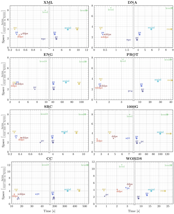
Figure 2: Running time and memory usage of the WT-constuction algorithms measured in seconds and bytes per byte of the input text, resp. Algorithms run on one core are marked with $\otimes$ whereas algorithms running on 32 cores are marked with $\times$.

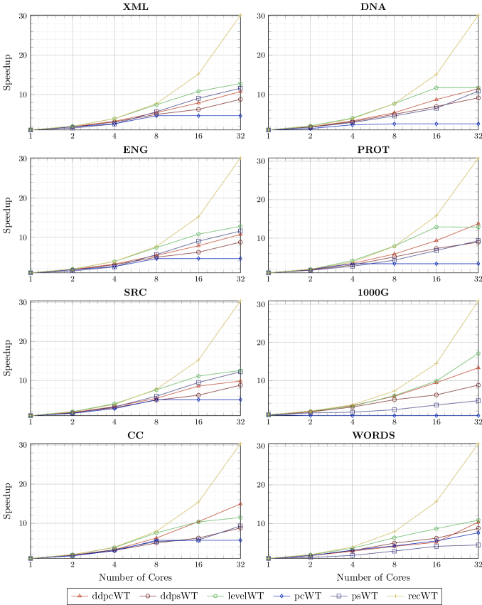
Figure 3: Comparison of the speedup of the WT-construction algorithms.

	ddWT				pWT
Text	$t_{1}$	$t_{32}$	$\text{m}_{1}$	$\text{m}_{32}$	$t_{1}$	$t_{32}$	$\text{m}_{1}$	$\text{m}_{32}$
XML	14.231	5.078	2.815	2.783	13.574	2.450	1.944	1.966
DNA	-	-	-	-	13.060	4.152	1.489	1.511
ENG	136.866	8.909	2.987	2.966	132.871	21.094	1.993	1.994
PROT	-	6.136	-	2.258	49.105	-	1.633	-
SRC	12.620	5.176	3.073	3.025	12.056	1.869	2.091	2.124
1000G	163.438	5.849	1.438	1.385	159.540	83.642	1.124	1.125
CC	-	24.0159	-	2.994	624.458	90.914	1.401	1.402
WORDS	26.386	9.563	2.786	2.803	26.666	3.673	1.869	1.883

Table 2: Experimental results of the WT-construction algorithms ddWT and pWT [7]. The experiments were conducted on the hardware and test instances that are described in §4. We measured the running time (in seconds) of the algorithms using one core ($t_{1}$) and 32 cores ($t_{32}$). The memory is given in bytes per byte of the input text when using one core ($\text{m}_{1}$) and 32 cores ($\text{m}_{32}$). A dash denotes that the algorithm could not compute the WT of the given text.

4.3.2 Memory Consumption.

The disadvantages of our algorithms when it comes to scaling are redeemed by their memory consumption, see again Figure 2. There we marked the number of bytes required per byte of input. The lowest memory consumption is achieved by pcWT, which matches our theoretical assumptions. Next, psWT requires 35 % more memory than pcWT, but still 27 % less than recWT when both are executed in parallel. In the sequential case, pcWT and psWT require 50 % and 25 % less space than serialWT. Our domain decomposition algorithms also match their expected memory consumption, as they require the same space as the algorithm used for the construction of the partial WTs in addition to a bit vector of the size of the text used for merging the partial WTs. (If psWT is used to compute the partial WTs, the space used for sorting of the text slices can be reused for the merging.) The memory consumption of levelWT is enormous, requiring around 77 % more memory than pcWT in both cases (sequential and parallel).

In practice, our algorithms require less memory than their competitors (with WORDS being the only exception). One reason is that our competitors use multiple arrays of text size to speed up the computation.

5 The Wavelet Matrix

A variant of the WT, the wavelet matrix (WM), was introduced in 2011 by Claude et al. [2]. It requires the same space as a WT and has the same asymptotic running times for access, rank, and select; but in practice it is often faster than a WT for rank and select queries [2], as it needs less calls to binary rank/select data structures. However, the fact that the WM loses some nice structural properties of the WT makes it harder to parallelize its construction, as divide-and-conquer WT-construction algorithms, e. g. recWT [13], cannot simply be transformed to WMs.

For the definition of the WM, we need additional notations: Reversing the significance of the bits is denoted by $\mathop{}\mathopen{}\mathop{\text{reverse}}\mathopen{}$, e. g., $\mathop{}\mathopen{}\mathop{\text{reverse}}\mathopen{}\left((\mathtt{001})_{2}\right)=(\mathtt{100})_{2}$. The bit-reversal permutation of order $k$ (denoted by $\pi_{k}$) is a permutation of $[0,2^{k})$ with $\pi_{k}(i)=(\mathop{}\mathopen{}\mathop{\text{reverse}}\mathopen{}\left(\mathop{}\mathopen{}\mathop{\text{bits}}\mathopen{}\left(i\right)\right))_{2}$. For example, $\pi_{2}=(0,2,1,3)=((\mathtt{00})_{2},(\mathtt{10})_{2},(\mathtt{01})_{2},(\mathtt{11})_{2})$. $\pi_{k}$ and $\pi_{k+1}$ can be computed from another, as $\pi_{k+1}=(2\pi_{k}(0),\dots,2\pi_{k}(2^{k}-1),2\pi_{k}(0)+1,\dots,2\pi_{k}(2^{k}-1)+1)$ and $\pi_{k}=(\pi_{k+1}(0)/2,\dots,\pi_{k+1}(2^{k}-1)/2)$. In practice, we can realize the division by a single bit shift.

Wavelet Matrices.

The wavelet matrix (WM) [2] has only a single bit vector $\mathop{}\mathopen{}\mathsf{BV}\mathopen{}^{\prime}_{\ell}$ per level $\ell\in[0,\lceil\lg\sigma\rceil)$ like the level-wise WT, but the tree structure is discarded completely in the sense that we do not require each character to be represented in an interval that is covered by the character’s interval on the previous level. In addition, we use the array $\mathop{}\mathopen{}\mathsf{Z}\mathopen{}[0,\lceil\lg\sigma\rceil)$ to store the number of zeros at each level $\ell$ in $\mathop{}\mathopen{}\mathsf{Z}\mathopen{}[\ell]$.

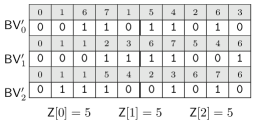
Figure 4: The WM of our running example, $\mathop{}\mathopen{}\mathsf{T}\mathopen{}=\mathtt{0167154263}$. The light gray ( ) arrays contain the characters represented at the corresponding position in the bit vector and are not a part of the WM. The thick lines highlight the number of zeros at each level.

$\mathop{}\mathopen{}\mathsf{BV}\mathopen{}^{\prime}_{0}$ contains the MSBs of each character in $\mathop{}\mathopen{}\mathsf{T}\mathopen{}$ in text order (this is the same as the first level of a WT). For $\ell\geq 1$, $\mathop{}\mathopen{}\mathsf{BV}\mathopen{}^{\prime}_{\ell}$ is defined as follows. Assume that a character $\alpha$ is represented at position $i$ in $\mathop{}\mathopen{}\mathsf{BV}\mathopen{}^{\prime}_{\ell-1}$. Then the position of its $\ell$-th MSB in $\mathop{}\mathopen{}\mathsf{BV}\mathopen{}^{\prime}_{\ell}$ depends on $\mathop{}\mathopen{}\mathsf{BV}\mathopen{}^{\prime}_{\ell-1}[i]$ in the following way: if $\mathop{}\mathopen{}\mathsf{BV}\mathopen{}^{\prime}_{\ell-1}[i]=0$, $\mathop{}\mathopen{}\mathop{\text{bit}}\mathopen{}\left(\ell,\alpha\right)$ is stored at position $\textnormal{{rank}}_{0}(\mathop{}\mathopen{}\mathsf{BV}\mathopen{}^{\prime}_{\ell-1},i)$; otherwise ($\mathop{}\mathopen{}\mathsf{BV}\mathopen{}^{\prime}_{\ell-1}[i]=1$), it is stored at position $\mathop{}\mathopen{}\mathsf{Z}\mathopen{}[\ell-1]+\textnormal{{rank}}_{1}(\mathop{}\mathopen{}\mathsf{BV}\mathopen{}^{\prime}_{\ell-1},i)$. For an example, see Figure 4.

Similar to the intervals in $\mathsf{BV}_{\ell}$ of the WT, characters of $\mathop{}\mathopen{}\mathsf{T}\mathopen{}$ form intervals in $\mathop{}\mathopen{}\mathsf{BV}\mathopen{}^{\prime}_{\ell}$ of the WM. Again, the intervals at level $\ell$ correspond to bit prefixes of size $\ell$, but due to the construction of the WM we consider the reversed bit prefixes. The simplicity of the change required to turn the previously discussed WT-construction algorithms in WM-construction algorithms are based on the following Observation:

Observation 2.

Given a character $\mathop{}\mathopen{}\mathsf{T}\mathopen{}[i]$ for $i\in[0,n)$ and a level $\ell\in[1,\lceil\lg\sigma\rceil)$ of the WM, the interval pertinent to $\mathop{}\mathopen{}\mathsf{T}\mathopen{}[i]$ in $\mathop{}\mathopen{}\mathsf{BV}\mathopen{}^{\prime}_{\ell}$ can be computed by $\mathop{}\mathopen{}\mathop{\text{reverse}}\mathopen{}\left(\mathop{}\mathopen{}\mathop{\text{prefix}}\mathopen{}\left(\ell,\mathop{}\mathopen{}\mathsf{T}\mathopen{}[i]\right)\right)$. Namely, $\mathop{}\mathopen{}\mathsf{BV}\mathopen{}^{\prime}_{\ell}[i]=\mathop{}\mathopen{}\mathop{\text{bit}}\mathopen{}\left(\ell,\mathop{}\mathopen{}\mathsf{T}\mathopen{}^{\prime}[i]\right)$, i. e., the $\ell$-th MSB of the $i$-th character of $\mathop{}\mathopen{}\mathsf{T}\mathopen{}^{\prime}$ in text order, where $\mathop{}\mathopen{}\mathsf{T}\mathopen{}^{\prime}$ is $\mathop{}\mathopen{}\mathsf{T}\mathopen{}$ stably sorted using the reversed bit prefixes of length $\ell$ of the characters as key.

As with WTs, if the bit vectors are augmented by (binary) rank and select data structures, the WM can be used to answer access, rank and select queries on a text over an alphabet of size $\sigma$ in $\mathop{}\mathopen{}\mathcal{O}\mathopen{}\left(\lg\sigma\right)$ time. We refer to [2] for a detailed description of these queries.

5.1 Adaption of our Algorithms to Wavelet Matrices.

When comparing the bit vectors of the WT and the WM at level $\ell$, we see two similarities. First, both bit vectors contain the $\ell$-th MSB of each character of $\mathop{}\mathopen{}\mathsf{T}\mathopen{}$ and second, the bits are grouped in intervals with respect to the bit prefix of size $\ell$ of the corresponding character and appear in the same order. Thus, the number and sizes of the intervals is the same. The difference is only the position of the intervals within each level. At level $\ell$, the intervals in $\mathsf{BV}_{\ell}$ of a WT occur in increasing order with respect to the bit prefixes of size $\ell$ of the characters in $\mathop{}\mathopen{}\mathsf{T}\mathopen{}$, i. e., the first interval corresponds to characters with bit prefix $0$, the second corresponds to characters with bit prefix $1$, and so on. The intervals in $\mathop{}\mathopen{}\mathsf{BV}\mathopen{}^{\prime}_{\ell}$ of a WM occur in increasing order with respect to the bit-reversal permutation $\pi_{\ell}$ of the characters in $\mathop{}\mathopen{}\mathsf{T}\mathopen{}$.

All our algorithms (pcWT, psWT, ddpcWT and ddpsWT) can be adjusted to compute the WM instead of the WT. We call them pcWM, psWM, ddpcWM and ddpsWM, respectively. To do so, we just have to replace the identity permutation by the bit reversal permutation $\pi$, i. e., choosing $id=\pi_{\ell}$ in lines 1 and 2 in Algorithms 1 and 2, resp. Then, the resulting starting positions of the intervals for bit prefixes are in bit reversal permutation order, i. e., the starting positions of the intervals for a WM (compare Observations 1 and 2).

	pc				ps				ddpc		ddpc
Text	$t_{1}$	$t_{32}$	$\text{m}_{1}$	$\text{m}_{32}$	$t_{1}$	$t_{32}$	$\text{m}_{1}$	$\text{m}_{32}$	$t_{32}$	$\text{m}_{32}$	$t_{32}$	$\text{m}_{32}$
XML	4.737	0.988	1.875	1.875	4.355	0.531	2.875	2.875	0.468	2.750	0.529	2.875
DNA	3.895	1.479	1.500	1.500	4.293	0.904	2.500	2.500	0.691	2.000	0.805	2.500
ENG	42.705	7.388	2.000	2.000	41.847	4.203	3.000	3.000	3.252	3.000	3.975	3.000
PROT	12.820	3.780	1.625	1.625	11.695	1.438	2.625	2.625	1.112	2.250	1.344	2.625
SRC	3.968	0.750	2.000	2.000	3.796	0.488	3.000	3.000	0.371	3.001	0.414	3.001
1000G	32.322	4.900	1.250	1.250	30.908	6.969	2.250	2.250	2.429	2.250	4.750	2.250
CC	191.166	33.893	2.000	2.000	203.923	15.817	3.000	3.000	13.798	3.000	16.180	3.000
WORDS	8.733	0.774	1.587	2.225	13.394	3.007	2.505	4.650	4.308	4.153	5.532	5.071

Table 3: Experimental results of our WM-construction algorithms described in §5.1. The hardware and test instances are described in §4. We measured the running time (in seconds) of the algorithms using one core ($t_{1}$) and 32 cores ($t_{32}$). The memory is given in bytes per byte of the input text when using one core ($\text{m}_{1}$) and 32 cores ($\text{m}_{32}$). Again, our algorithms based on domain decomposition use the corresponding sequential version of pcWM or psWM when run on one core.

In addition to the different order of the intervals, we also need to store the number of zeros. To this end, we use the starting positions of the intervals, as the number of zeros in any level is equal to even bit prefixes in the previous level. This requires additional $\lceil\lg\sigma\rceil\lceil\lg n\rceil$ bits of space and $\mathop{}\mathopen{}\mathcal{O}\mathopen{}\left(\sigma\right)$ time.

5.2 From the Wavelet Tree to the Wavelet Matrix.

We can also make use of these similarities by showing that every algorithm that can compute a WT can also compute a WM in the same asymptotic time.

Lemma 5.

We can compute in-place an array X and a bit vector U with rank and select data structures in time $\mathop{}\mathopen{}\mathcal{O}\mathopen{}\left(n+\sigma\right)$ and space $(n+\sigma)(1+o(1))+(\sigma+2)\lceil\lg n\rceil$ bits, such that $\mathsf{BV}_{\ell}[i]=\mathop{}\mathopen{}\mathsf{BV}\mathopen{}^{\prime}_{\ell}[j]$ with

$$j=\begin{cases}i&,\text{if\leavevmode\nobreak\ }\ell\leq 1\\ \mathsf{X}[2^{\ell-1}-2+bp]+\text{off}&,\text{otherwise}\end{cases}$$

where $bp=\mathop{\mathrm{prefix}}(\ell,\textnormal{{rank}}_{0}(\mathsf{U},\textnormal{{select}}_{1}(\mathsf{U},i+1)))$ and $\text{off}=i-\textnormal{{rank}}_{1}(\mathsf{U},\textnormal{{select}}_{0}(\mathsf{U},bp\ll(\lceil\lg\sigma\rceil-\ell)))$, with $\ll k$ denoting a left bit shift (by $k$ bits), i. e., affixing $k$ zeros on the right hand side.

Proof.

We require two auxiliary data structures for the transformation. The first one is the bit vector $\mathsf{U}$ of length $n+\sigma$ that stores the unary representation of the histogram of all characters in $\mathop{}\mathopen{}\mathsf{T}\mathopen{}$. The second one is an array $\mathsf{X}$ of size $(\sigma+2)\lceil\lg n\rceil$ bits, which at first is used for counting, and later on stores the starting positions of all intervals in the WM.

To compute $\mathsf{U}$ we first count the number of occurrences of all characters and store them in $\mathsf{X}$ such that $\mathsf{X}[i]=|\{j\in[0,n)\colon\mathop{}\mathopen{}\mathsf{T}\mathopen{}[j]=i\}|$ for all $i\in[0,\sigma)$. Then, the unary histogram is given by $\mathsf{U}=1^{\mathsf{X}[\mathtt{0}]}\mathtt{01}^{\mathsf{X}[1]}\mathtt{0}\dots\mathtt{1}^{\mathsf{X}[\sigma-1]}$. In addition, we augment $\mathsf{U}$ with a rank/select data structure. All this requires $\mathop{}\mathopen{}\mathcal{O}\mathopen{}\left(n+\sigma\right)$ time and $o(n+\sigma)$ bits space in addition to $\mathsf{U}$ and $\mathsf{X}$.

Next, we want to compute the starting positions of the intervals in the WM (i. e., fill the array $\mathsf{X}$ with its final content). We require those for intervals corresponding to bit prefixes of size $\ell$ with $\ell\in[1,\lceil\lg\sigma\rceil)$, i. e., for all but the first level of the WM. To this end, we compute the number of occurrences of characters that share a bit prefix of size $\lceil\lg\sigma\rceil-1$ in the first $\lceil\sigma/2\rceil-1$ positions of $\mathsf{X}$. With the histogram information still in $\mathsf{X}$, this can be done by setting $\mathsf{X}[i]=\mathsf{X}[2i]+\mathsf{X}[2i+1]$ for all $i\in[0,\lceil\sigma/2\rceil)$ in increasing order. We set all other positions of X to zero. Next, we compute the zero based prefix sum with respect to $\pi_{\lceil\lg\sigma\rceil-1}$ of the first $\lceil\sigma/2\rceil-1$ entries of X and in the last $\lceil\sigma/2\rceil-1$ entries of X. Here, “respect to $\pi_{\lceil\lg\sigma\rceil-1}$” means that character $\pi_{\lceil\lg\sigma\rceil-1}(i)$ follows character $\pi_{\lceil\lg\sigma\rceil-1}(i-1)$ for all $i\in[1,\lceil\sigma/2\rceil)$. In the same fashion, we compute the starting positions of the intervals in all other levels. (By first computing the number of occurrences of bit prefixes of size $k$ using the ones of size $k+1$ and storing the zero based prefix sum with respect to $\pi_{\lceil\lg k\rceil}$ in the rightmost free entries of X.) The $\sigma+2$ entries (of size $\lceil\lg n\rceil$) in X are sufficient for this. Since the first entries of X can be empty (depending on $\sigma$), we finally move the starting positions to the left, such that the first starting position is stored in $\mathsf{X}[0]$. All this can be done in $\mathop{}\mathopen{}\mathcal{O}\mathopen{}\left(\sigma\right)$ time without any additional space. Therefore, the construction of U (its augmenting rank/select data structure) and X requires $\mathop{}\mathopen{}\mathcal{O}\mathopen{}\left(n+\sigma\right)$ time and $(n+\sigma)(1+o(1))+(\sigma+2)\lceil\lg n\rceil$ bits of space (including U and X).

Now we need to answer queries asking for a position $j\in[0,n)$ in $\mathop{}\mathopen{}\mathsf{BV}\mathopen{}^{\prime}_{\ell}$ given a position $i\in[0,n)$ in $\mathsf{BV}_{\ell}$ for $\ell\in[0,\lceil\lg\sigma\rceil)$ in constant time, i. e., the position $j$ in the WM corresponding to the position $i$ in the WT. If $\ell\leq 1$ we know that $j=i$, because the bit vectors of the WT and WM are the same for the first two levels. Otherwise ($\ell>1$), the computation of the position $j$ consists of two steps. First, we determine the starting position of the interval in the WM (using $\mathsf{X}$). Second, we compute the number of entries in the interval existing before $i$ (which is the same for WM and WT, as the intervals are the same):

1. We first need to identify the bit prefix of length $\ell$ corresponding to the interval containing $i$. Note that we are only interested in the bit prefix and not in the character $c$ corresponding to position $i$. There are at least $i-1$ (or none, if $i=0$) characters occurring in $\mathop{}\mathopen{}\mathsf{T}\mathopen{}$ whose bit prefix of length $\ell$ is at most $\mathop{}\mathopen{}\mathop{\text{prefix}}\mathopen{}\left(\ell,c\right)$. (There are more than $i-1$ characters if at least one character with bit prefix $\mathop{}\mathopen{}\mathop{\text{prefix}}\mathopen{}\left(\ell,c\right)$ occurs after $c$ in $\mathop{}\mathopen{}\mathsf{T}\mathopen{}$.) Therefore, $c^{\prime}=\textnormal{{rank}}_{0}(\mathsf{U},\textnormal{{select}}_{1}(\mathsf{U},i+1))$ has the same bit prefix of length $\ell$ as $c$, i. e., $bp=\mathop{}\mathopen{}\mathop{\text{prefix}}\mathopen{}\left(\ell,c^{\prime}\right)=\mathop{}\mathopen{}\mathop{\text{prefix}}\mathopen{}\left(\ell,c\right)$. Since we have stored all starting positions of the intervals on level $\ell$ in the WM in $\mathsf{X}[2^{\ell}-2,2^{\ell+1})$ the starting position is $\mathsf{X}[2^{\ell}-2+bp]$.

2. Now we need to compute the offset of the position from the starting position of the interval. To do so, we compute the smallest character contained in the interval by padding the bit prefix with $\lceil\lg\sigma\rceil-\ell$ 0’s giving us a value $r=\textnormal{{select}}_{0}(\mathsf{U},bp\ll\lceil\lg\sigma\rceil-\ell)$. Next, we determine the number of 1’s occurring before the $r$-th 0 in $\mathsf{U}$ to compute the offset, i. e., $\textit{off}=i-\textnormal{{rank}}_{1}(\mathsf{U},r).$

Since all operations used for querying require constant time and there is only a constant number of operations, the query can be answered in constant time. ∎

6 Conclusions

We presented new sequential and parallel wavelet tree (and matrix) construction algorithms. Their unifying feature is their bottom-up approach, which saves repeated histogram computations per level from scratch and is also responsible for their space consciousness. Our experiments showed that our new sequential algorithms are up to twice as fast as the previously known algorithms while requiring just a fraction of the memory (at most half as much). In addition to the practical work, we also have shown how to (theoretically) adopt general WT-construction algorithms to compute a WM in the same asymptotic runtime.

The presented algorithms are the first practical parallel WM-construction algorithms. It remains an open problem how to design parallel algorithms for wavelet matrices that scale as well as the best one for wavelet trees [13].

References

- [1] Maxim A. Babenko, Pawel Gawrychowski, Tomasz Kociumaka, and Tatiana A. Starikovskaya. Wavelet trees meet suffix trees. In Annual ACM-SIAM Symposium on Discrete Algorithms (SODA), pages 572–591. SIAM, 2015.
- [2] Francisco Claude, Gonzalo Navarro, and Alberto Ordóñez Pereira. The wavelet matrix: An efficient wavelet tree for large alphabets. Inf. Syst., 47:15–32, 2015.
- [3] Francisco Claude, Patrick K. Nicholson, and Diego Seco. Space efficient wavelet tree construction. In International Symposium on String Processing and Information Retrieval (SPIRE), volume 7024 of LNCS, pages 185–196. Springer, 2011.
- [4] Paulo G. S. da Fonseca and Israel B. F. da Silva. Online construction of wavelet trees. In International Symposium on Experimental Algorithms (SEA), volume 75 of LIPIcs, pages 16:1–16:14. Schloss Dagstuhl - Leibniz-Zentrum für Informatik, 2017.
- [5] Paolo Ferragina, Raffaele Giancarlo, and Giovanni Manzini. The myriad virtues of wavelet trees. Inf. Comput., 207(8):849–866, 2009.
- [6] José Fuentes-Sepúlveda, Erick Elejalde, Leo Ferres, and Diego Seco. Efficient wavelet tree construction and querying for multicore architectures. In International Symposium on Experimental Algorithms (SEA), volume 8504 of LNCS, pages 150–161. Springer, 2014.
- [7] José Fuentes-Sepúlveda, Erick Elejalde, Leo Ferres, and Diego Seco. Parallel construction of wavelet trees on multicore architectures. Knowl. Inf. Syst., 51(3):1043–1066, 2017.
- [8] Simon Gog, Timo Beller, Alistair Moffat, and Matthias Petri. From theory to practice: Plug and play with succinct data structures. In International Symposium on Experimental Algorithms (SEA), pages 326–337, 2014.
- [9] Simon Gog, Juha Kärkkäinen, Dominik Kempa, Matthias Petri, and Simon J. Puglisi. Faster, minuter. In Data Compression Conference (DCC), pages 53–62, 2016.
- [10] Roberto Grossi, Ankur Gupta, and Jeffrey Scott Vitter. High-order entropy-compressed text indexes. In Annual ACM-SIAM Symposium on Discrete Algorithms (SODA), pages 841–850. SIAM, 2003.
- [11] Roberto Grossi, Jeffrey Scott Vitter, and Bojian Xu. Wavelet trees: From theory to practice. In International Conference on Data Compression, Communications and Processing (CCP), pages 210–221. IEEE, 2011.
- [12] Joseph JáJá. An Introduction to Parallel Algorithms. Addison-Wesley, 1992.
- [13] Julian Labeit, Julian Shun, and Guy E. Blelloch. Parallel lightweight wavelet tree, suffix array and FM-index construction. In Data Compression Conference (DCC), pages 33–42. IEEE, 2016.
- [14] Veli Mäkinen and Gonzalo Navarro. Position-restricted substring searching. In Latin American Theoretical Informatics Symposium (LATIN), volume 3887 of LNCS, pages 703–714. Springer, 2006.
- [15] Veli Mäkinen and Gonzalo Navarro. Rank and select revisited and extended. Theor. Comput. Sci., 387(3):332–347, 2007.
- [16] Christos Makris. Wavelet trees: A survey. Comput. Sci. Inf. Syst., 9(2):585–625, 2012.
- [17] J. Ian Munro, Yakov Nekrich, and Jeffrey Scott Vitter. Fast construction of wavelet trees. Theor. Comput. Sci., 638:91–97, 2016.
- [18] Gonzalo Navarro. Wavelet trees for all. J. Discrete Algorithms, 25:2–20, 2014.
- [19] Benedikt Oesing. Effiziente Erstellung von Waveletmatrizen (B. Sc. Thesis in German), 2016.
- [20] Julian Shun. Parallel wavelet tree construction. In Data Compression Conference (DCC), pages 63–72. IEEE, 2015.
- [21] Julian Shun. Improved parallel construction of wavelet trees and rank/select structures. In Data Compression Conference (DCC), pages 92–101. IEEE, 2017.
- [22] German Tischler. On wavelet tree construction. In Annual Symposium on Combinatorial Pattern Matching (CPM), volume 6661 of LNCS, pages 208–218. Springer, 2011.