Mutual Uncertainty, Conditional Uncertainty and Strong Sub-Additivity

Abstract

We introduce a new concept called as the mutual uncertainty between two observables in a given quantum state which enjoys similar features like the mutual information for two random variables. Further, we define the conditional uncertainty as well as conditional variance and show that conditioning on more observable reduces the uncertainty. Given three observables, we prove a ‘strong sub-additivity’ relation for the conditional uncertainty under certain condition. As an application, we show that using the conditional variance one can detect bipartite higher dimensional entangled states. The efficacy of our detection method lies in the fact that it gives better detection criteria than most of the existing criteria based on geometry of the states. Interestingly, we find that for $N$-qubit product states, the mutual uncertainty is exactly equal to $N-\sqrt{N}$, and if it is other than this value, the state is entangled. We also show that using the mutual uncertainty between two observables, one can detect non-Gaussian steering where Reid’s criteria fails to detect. Our results may open up a new direction of exploration in quantum theory and quantum information using the mutual uncertainty, conditional uncertainty and the strong sub-additivity for multiple observables.

I Introduction

In quantum theory, Heisenberg’s uncertainty relation whu restricts the knowledge of physical observables one can have about the quantum system. The Heisenberg-Robertson uncertainty hpru ; kenn ; book1 ; uncert_review relation suggests the impossibility of preparing an ensemble where one can measure two non-commuting observables with infinite precisions. Later, Schrödinger esu improved the lower bound of this uncertainty relation. In fact, Robertson and Schrödinger formulated mathematically the uncertainty relation for any two observables. Recently, the stronger uncertainty relations have been proved which go beyond the Robertson-Schrödinger uncertainty relation str-ur1 and this has strengthened the notion of incompatible observables in quantum theory str-ur2 ; str-ur3 ; str-ur4 ; str-ur5 ; str-ur6 ; str-ur7 .

Shannon introduced entropy as a measure of information contained in a classical random variable shannon-ent . The introduction of entropy paved a path for a new field “Classical Information Science” info . Later, von Neumann extended the idea of entropy to the quantum domain where one replaces the probability distribution of random variables with the density operators for the states of quantum systems. Undoubtedly, entropy is an important quantity in quantum information science qinfo ; wilde-book . As entropy measures lack of information about the preparation of a system, one can also express uncertainty relations in terms of entropies entro-unce ; rev-entro . However, in the quantum world, variance of an observable is also a measure of lack of information about the state preparation huang . Therefore, it may be natural to ask if using the variance as uncertainty measure, one can define analogous quantities such as the mutual information, the conditional entropy and the notion of strong sub-additivity.

Once we define these quantities, one immediate question is: Do they provide new insights about the quantum systems. The answer to this is in affirmative. For example, the mutual information, is the corner stone in defining many important aspects in information theory, like, unveiling correlations, channel capacities etc in quantum information science qinfo ; wilde-book . The conditional entropy is also inevitably an important quantity which is relevant in quantum communication as well as quantum computation qinfo ; wilde-book . While these analogies are very tempting to address for quantum uncertainty related quantities, there is a major departure between these two notions. The uncertainty is a function of both a quantum state and an observable whereas the notion of entropy depends on either of the two qinfo ; wilde-book . Moreover, while the uncertainty captures only the second moment, the entropy contains all the possible moments.

In this paper, we introduce the notion of mutual uncertainty, conditional uncertainty and strong sub-additivity on the basis of quantum uncertainties expressed in terms of standard deviations and variances. Interestingly, we find that the standard deviation (quantum uncertainty) behaves in many ways like entropy. For example, we find that a chain rule for the sum uncertainty holds. Due to this fact one can easily define many important quantities like conditional mutual uncertainty as well. Another important aspect of this formalism is that one can have a version of ‘strong subadditivity (SSA)’ for quantum uncertainties which may have implications in quantum information and this may be of independent interest. Also, we prove the strong subadditivity for more than three observables using the mutual uncertainty.

Then, we address the physical implication of all these quantities introduced here. As illustrations, we consider two important aspects in quantum information science – detecting entanglement entrev ; entdetrev ; corr-rev as well as quantum steering steer1 . We find that using the conditional variance, we can detect entanglement of higher dimensional bipartite mixed state. The method we present here is stronger than the criteria found by Vicente high_ent1 . Moreover, we find that for $N$-qubit product states, the mutual uncertainty is exactly equal to $N-\sqrt{N}$. This provides a sufficient condition to detect $N$-qubit entanglement. The other important finding is that we derive a steering criteria based on the mutual uncertainty. This criteria is as powerful as Reid’s steering criteria MDsteer for two qubits, and overpowers it when we consider non-Gaussian bipartite states. These results show the efficacy of our formalism. In fact, from the perspective of experimental realizations, our formalism might be one step ahead of the usual entropic formalism because, variances are easy to measure experimentally compared to entropic quantities which cannot be measured directly.

The paper is organized as follows. In the next section, we discuss the sum uncertainty relation. Then, we define mutual uncertainty, conditional uncertainty and derive some important identities and inequalities like the chain rule, the strong subadditivity of uncertainties in section-III. In section-IV, we study the physical implication of these quantities, namely, usefulness of the conditional variance in detecting entangled states and finding steerable states using the mutual uncertainty. We conclude in the last section.

II Setting the stage: Sum uncertainty relations

Let us consider a set of observables represented by Hermitian operators $\{A_{i}\}$, then the uncertainty of $A_{i}$ in a given quantum state $\rho$ is defined as the statistical variance ($\triangle^{2}$) or standard deviation ($\triangle$) of the corresponding observable, i.e., $\triangle A_{i}^{2}=\langle A_{i}^{2}\rangle-\langle A_{i}\rangle^{2}$, where $\langle A_{i}\rangle=\operatorname{Tr}[\rho A_{i}]$ for the state $\rho$. This positive quantity can only be zero if $\rho$ is an eigenstate of $A_{i}$, representing the exact predictability of the measurement outcome. Hence, a quantum state with zero uncertainty must be a simultaneous eigenstate of all $A_{i}$’s. The “sum uncertainty relation” arun1 tells us that the sum of uncertainty of two observables is greater or equals to the uncertainty of the sum of the observables on a quantum system. If $A$ and $B$ are two general observables that represent some physical quantities, then one may ask: What is the relation between $\triangle(A+B)$, $\triangle A$, and $\triangle B$? The following theorem answers this.
Theorem.1 arun1 : Quantum fluctuation in the sum of any two observables is always less than or equal to the sum of their individual fluctuations, i.e., $\triangle(A+B)\leq\triangle A+\triangle B$.

The theorem was proved for pure states only but one can easily extend the result for the arbitrary mixed states by employing the purification of the mixed states in higher dimensional Hilbert space. The physical meaning of the sum uncertainty relation is that if we have an ensemble of quantum systems then the ignorance in totality is always less than the sum of the individual ignorances. In the case of two observables, if we prepare a large number of quantum systems in the state $\rho$, and then perform the measurement of $A$ on some of those systems and $B$ on some others, then the standard deviations in $A$ plus $B$ will be more than the standard deviation in the measurement of $(A+B)$ on those systems. Hence, it is always advisable to go for the ‘joint measurement’ if we want to minimize the error. Another aspect of this theorem is that it is similar in spirit to the subadditivity of the von Neumann entropy, i.e., $S(\rho_{12})\leq S(\rho_{1})+S(\rho_{2})$, where $\rho_{12}$ is a two particle density operator and $\rho_{2}$=$\operatorname{Tr}_{1}(\rho_{12})$ is the reduced density for subsystem $2$. Noticing this resemblance of quantum entropy and standard deviation measure of uncertainty, it is tempting to see if we can unravel some other features. Before doing that we will first summarize the properties of the uncertainty (captured by standard deviation) arun1 .

Properties of $\triangle(\cdot)$: (i) $\triangle A_{i}\geq 0$ for $\{A_{i}\}$ in $\rho$, (ii) It is convex in nature, i.e., $\triangle(\sum_{i}p_{i}A_{i})\leq\sum_{i}p_{i}\triangle(A_{i})$, with $0\leq p_{i}\leq 1$ and $\sum_{i}p_{i}=1$ and (iii) one cannot decrease the uncertainty of an observable by mixing several states $\rho=\sum_{\ell}\lambda_{\ell}\rho_{\ell}$, i.e., $\triangle(A)_{\rho}\geq\sum_{\ell}\lambda_{\ell}\triangle(A)_{\rho_{\ell}}$, with $\sum_{\ell}\lambda_{\ell}=1$. This is similar to the fact that entropy is also a concave function of the density matrices, i.e., $S(\sum_{\ell}\lambda_{\ell}\rho_{\ell})\geq\sum_{\ell}\lambda_{\ell}S(\rho_{\ell})$.

In fact, it is not difficult to see that if we have more than two observables (say three observables $A$, $B$, and $C$), then the sum uncertainty relation will read as $\triangle(A+B+C)\leq\triangle A+\triangle B+\triangle C$. In general, for observables $\{A_{i}\}$, we will have the sum uncertainty relation as $\triangle(\sum_{i}A_{i})\leq\sum_{i}\triangle A_{i}$ arun1 .

III Mutual uncertainty

For any two observable A and B, the mutual uncertainty in the quantum state $\rho$ is defined as

$$M(A:B):=\triangle A+\triangle B-\triangle(A+B).$$ (1)

We name $M(A:B)$ as the mutual uncertainty in the same spirit as that of the mutual information. (The mutual information for a bipartite state $\rho_{12}$ is defined as $I(\rho_{12})=S(\rho_{1})+S(\rho_{2})-S(\rho_{12})$.) The quantity $M(A:B)$ captures how much overlap two observables can have in a given quantum state.
Properties of $M(A:B)$: (i) $M(A:B)\geq 0$, (ii) it is symmetric in $A$ and $B$, i.e., $M(A:B)=M(B:A)$, and (iii) $M(A:A)=0$. Note that $I(\rho_{12})$ also satisfies similar properties.
The above definition of mutual uncertainty can be generalized for $n$ number of observables. Thus, given a set of observables $\{A_{i};i=1,2,...,n\}$, we have

$$M(A_{1}:A_{2}:\cdots:A_{n}):=\sum_{i=1}^{n}\triangle A_{i}-\triangle(\sum_{i=1}^{n}A_{i}).$$ (2)

The above relation is analogous to the mutual information for $n$-particle quantum state $\rho_{12..n}$ which is defined as $I(\rho_{12..n})=\sum_{i=1}^{n}S(\rho_{i})-S(\rho_{12...n})$ note2 .

Note that all the observables may not have same physical dimension but one can make them of same dimension by multiplying them with proper dimensional quantities. Although in this article we have omitted this possibility by considering dimensionless observables.

III.1 Conditional uncertainty and chain rule for uncertainties

We define a new quantity called the conditional uncertainty (similar to the conditional entropy $S(\rho_{1|2})=S(\rho_{12})-S(\rho_{2})$) as

$$\triangle(A|B): = \triangle(A+B)-\triangle B.$$ (3)

This suggest that how much uncertainty in $(A+B)$ remains after we remove the uncertainty in $B$.
Properties of $\triangle(A|B)$: (i)$\triangle(A|B)\leq\triangle A$, i.e., conditioning on more observables reduces the uncertainty. (ii) $\triangle(A|B)\geq 0$ but can be negative if $\triangle(A+B)<\triangle B$ or vice versa, (iii) $\triangle(A|A)=\triangle A$.
By noting that $\triangle(A|B)=\triangle A-M(A:B)$ and $M(A:B)\geq 0$, we have property (i). A simple example will illustrate the property (ii) note-ve .

Now we will derive some useful results using the mutual uncertainty and the conditional uncertainty.
Theorem.2 Chain rule for the sum uncertainty holds, i.e., $\triangle\left(\displaystyle\sum_{i=1}^{n}A_{i}\right)=\displaystyle\sum_{i=1}^{n}\triangle(A_{i}|A_{i-1}+\cdot\cdot\cdot+A_{1})$.

Proof.

For three observables, the chain rule reads as

$$\triangle(A+B+C)=\triangle A+\triangle(B|A)+\triangle(C|A+B).$$

Now consider

$$RHS = \triangle A+\triangle(B|A)+\triangle(C|A+B)$$

$$= \triangle A+\triangle(B|A)+\triangle(C+A+B)-\triangle(A+B)$$

$$= \triangle(C+A+B)=LHS.$$

Similarly, one can prove by mathematical induction, that the theorem holds for all positive integer $n$. ∎

This tells us that the sum uncertainty of two observable is equal to the uncertainty of one observable plus the conditional uncertainty of the other observables, i.e., $\triangle(A+B)=\triangle(A)+\triangle(B|A)$ which is similar to the entropy of the joint random variables or the bipartite systems. We can also define the following quantity as well.
Conditional mutual uncertainty.– We define another quantity which we call the conditional mutual uncertainty in the same spirit of the conditional mutual information. This is defined as $M(A:B|C):=\triangle(A|C)+\triangle(B|C)-\triangle(A+B|C)$, which can be simplified as

$$M(A:B|C)=\triangle(B|C)-\triangle(B|C+A),$$ (4)

using the chain rule for the mutual uncertainty.

III.2 Strong sub-additivity like relations

The strong sub-additivity of entropy is an important result in information science. It gives a fundamental limitation to the distribution of entropy in a composite system araki-lieb ; lieb-ruskai . In classical case it implies the non-negativity of the mutual information. For the relative entropy based quantum mutual information, $I(\rho_{12..n})=S(\rho_{12..n}||\otimes_{i=1}^{n}\sigma_{i})$ m-mutual-rela , the strong sub-additivity of entropy guarantees the positivity posi-mu-m but not for the other versions of mutual information posi-mu-m1 . In a broad sense, the strong sub-additivity of entropy implies that the conditioning will not increase the entropy, i.e., $S(\rho_{1|23})\leq S(\rho_{1|2})$. Moreover, beyond three particle systems we do not know the actual form of strong sub-additivity of quantum entropy.
Here, we will prove a strong sub-additivity like relation concerning the uncertainties for multiple observables in a given quantum state.
Theorem.3 If $M(B:C)=0$, then $\triangle(A|B+C)\leq\triangle(A|B)$, i.e., conditioning on more observables reduces the uncertainty.

Proof.

Lets start with the sum uncertainty relation, i.e.,

$$\triangle(A+B+C) \leq \triangle(A+B)+\triangle C$$

$$\triangle(A+B+C)-\triangle(B+C) \leq \triangle(A+B)-\triangle B+\triangle B$$

$$+\triangle C-\triangle(B+C)$$

$$\triangle(A|B+C) \leq \triangle(A|B)+M(B:C)$$

Hence, the proof. ∎

The above relation can be understood as the “Strong Sub-Additivity” of uncertainty. The strong sub-additivity relation for uncertainty also ensures that the mutual uncertainty is always positive. For arbitrary number of observables, the strong sub-additivity relation says that if $M(A_{2}+\cdot\cdot\cdot+A_{n-1}:A_{n})=0$, then $\triangle(A_{1}|A_{2}+\cdot\cdot\cdot+A_{n})\leq\triangle(A_{1}|A_{2}+\cdot\cdot\cdot+A_{n-1})$.

Next, we will prove two important relations concerning the mutual uncertainty.
Inequality.1 Discarding the observable, one cannot increase the mutual uncertainty, i.e., $M(A:B)\leq M(A:B+C)$.

Proof.

To prove this, let us start with the quantity $M(A:B+C)$.

$$M(A:B+C)=\triangle A+\triangle(B+C)-\triangle(A+B+C)$$

$$\triangle(A+B+C)=\triangle A+\triangle(B+C)-M(A:B+C)$$

$$\leq\triangle A+\triangle B+\triangle C-M(A:B+C)$$

$$\leq M(A:B)+\triangle(A+B)+\triangle C-M(A:B+C)$$

$$\leq(\triangle A+\triangle B+\triangle C)-(M(A:B+C)-M(A:B)).$$

Using the sum uncertainty relation for three observables

$$\triangle(A+B+C)\leq\triangle A+\triangle B+\triangle C$$

and Eq.(III.2), we get

$$M(A:B+C)-M(A:B))\geq 0.$$

Hence the proof. ∎

This is another form of strong sub-additivity in terms of mutual uncertainty. Interestingly, mutual information also satisfies $I(\rho_{12})\leq I(\rho_{1(23)})$ info . Similarly, there is another total correlation measure, called as the entanglement of purification purif , that satisfies $E(\rho_{12})\leq E(\rho_{1(23)})$ puriarn . These observations provide added motivation to explore these new quantities in a greater details.

All these inequalities resemble with the well known inequalities concerning the entropy which are the corner stone of quantum information science. However, we note that these similarities are structural, actual interpretations of these inequalities might be completely different.

Conditional variance.– Here, we define the conditional variance (similar to the conditional entropy) as

$$\triangle(A|B)^{2}:=\triangle(A+B)^{2}-\triangle{B}^{2}.$$ (5)

This quantity is equivalent to $\triangle A^{2}+2\operatorname{Cov}(A,B)$, where $\operatorname{Cov}(A,B)=\frac{1}{2}\operatorname{Tr}[\rho(AB+BA)]-\operatorname{Tr}[\rho A]\operatorname{Tr}[\rho B]$ is the covariance of $A$ and $B$. It says that if the covariance is nonzero then the uncertainty in $A$ may increase or decrease due to the knowledge of the uncertainty of $B$ as covariance can take both positive (correlation) and negative (anti-correlation) values. This is in some sense different from the conditional uncertainty.

IV Physical implications

In this section, we will focus on some applications of the quantities we introduced in the main text, eg., the mutual uncertainty, the conditional uncertainty and the conditional variance. We will study these quantities for discrete systems such as the qubit-systems as well as higher dimensional systems, and the continuous variable systems also.

IV.1 Detection of entangled states

Entanglement is a crucial resource for many quantum information protocols (e.g., see entrev ). Hence, detection and quantification of entanglement is an important task. Several ways to detect entanglement have been proposed in the recent past entdetrev . In the literature, the uncertainty relations have been employed to detect entanglement where operators can be either locally applied on the subsystems hofmann or globally applied on the system as a whole guehne . This motivates us to ask the natural question here: Can we detect entanglement using the conditional variance or other introduced quantities here? In the subsequent analysis, we answer this question in affirmative.

There exists many elegant methods to detect entanglement using the local uncertainty relations hofmann ; high_ent4 ; high_ent7 ; highD_Bloch_sep or using geometry of quantum states cove1 ; maxE ; local ; high_ent1 ; high_ent2 ; high_ent3 ; high_ent5 ; high_ent6 . It is worthwhile to mention that using local uncertainty relations, one can detect more general form of entanglement, known as generalized entanglement which includes standard entanglement as special case sugg_1 ; sugg_2 ; sugg_3 ; sugg_4 .

In the following we use the conditional variance to derive a criteria which will detect the entanglement of two qudit mixed states. We find that the criteria based on the conditional variance is better than the existent criteria based on the geometry of the quantum states high_ent1 ; high_ent4 ; high_ent5 ; high_ent6 ; high_ent7 . We also consider $N$-qubit pure states and find a sufficient criteria of detecting its entanglement using the mutual uncertainty.

Bloch representation of $N$-particle quantum systems and the condition for its separability.– To express quantum states in higher dimension geometrically, one need to understand the structure of $SU(d)$ group. It contains $d^{2}-1$ generators termed as $\sigma_{i}$, which form the basis of the Lie algebra with commutation and anti-commutation relations respectively

$$[\sigma_{i},\sigma_{j}]=2i\sum_{k}f_{ijk}\sigma_{k},~{}~{}~{}~{}~{}~{}~{}$$

$$\{\sigma_{i},\sigma_{j}\}=\frac{4}{d}\delta_{ij}+2\sum_{k}d_{ijk}\sigma_{k}.$$

Here $f_{ijk}$ and $d_{ijk}$ are the anti-symmetric and symmetric structure constants. All $\sigma_{i}$ are traceless Hermitian matrices which satisfy $\sigma_{i}\sigma_{j}=\frac{2}{d}\delta_{ij}\mathbb{I}_{d}+\sum_{k}\left(if_{ijk}+d_{ijk}\right)\sigma_{k}$. For $d=2$, the symmetric structure constants, $d_{ijk}$ are ideally zero and the generators are well known Pauli matrices whereas for $d=3$, the generators are Gell-Mann matrices.

Any arbitrary single particle quantum state in $d$-dimension can be expressed as $\varrho=\frac{1}{d}\mathbb{I}_{d}+\frac{1}{2}\vec{r}.\vec{\sigma},$ where $\mathbb{I}_{n}$ is the identity matrix of order $n$ and $|\vec{r}|^{2}\leq\frac{2(d-1)}{d}$. The density matrix, $\varrho$, is a Hermitian matrix with $\varrho\geq 0$, $\varrho\geq\varrho^{2}$ (equality holds when $\varrho$ is pure) and ${\rm Tr}[\varrho]=1$.

The $N$-qudit state can be expressed in the generalized Bloch vector representation as

$$\rho=\frac{1}{d^{N}}\mathbb{I}_{d^{N}}+\frac{1}{2d^{N-1}}[\vec{\sigma}.\vec{r}\otimes\mathbb{I}_{d}^{\otimes N-1}+\cdots+\mathbb{I}_{d}^{\otimes N-1}\otimes\vec{\sigma}.\vec{r_{N}}]+\frac{1}{4d^{N-2}}\sum_{ij}[t_{ij0\cdots 0}\sigma_{i}\otimes\sigma_{j}\otimes\mathbb{I}_{d}^{\otimes N-2}+\cdots$$

$$+t_{0\cdots 0ij}\mathbb{I}_{d}^{\otimes N-2}\otimes\sigma_{i}\otimes\sigma_{j}]+\cdots+\frac{1}{2^{N}}\sum_{i_{1}\cdots i_{N}}t_{i_{1}\cdots i_{N}}\sigma_{i_{1}}\otimes\cdots\otimes\sigma_{i_{N}},~{}~{}~{}~{}~{}~{}~{}~{}~{}~{}~{}~{}~{}~{}~{}~{}~{}~{}~{}~{}~{}~{}~{}~{}~{}~{}~{}~{}~{}~{}~{}~{}~{}~{}$$ (6)

where $\vec{r_{i}}$ are the Bloch vector for the $i^{th}$ subsystem, $\{[t_{ij0\cdots 0}],\cdots,[t_{0\cdots 0ij}]\}$ are pairwise correlation tensors, and $[t_{i_{1}\cdots i_{N}}]$ is the $N$-way correlation tensor. The are other type of correlation tensors, like, $3$-way, $4$-way, $\cdots$, $N-1$-way, which will not play a role in our analysis. For notational simplicity, we will call $T^{(k)}$ as $k$-way correlation tensor, where for example, $T^{(2)}$ forms a set $\{[t_{ij0\cdots 0}],\cdots,[t_{0\cdots 0ij}]\}$ and so on. The conditions required to approve the above matrix as a valid density matrix are – $|\vec{r_{i}}|^{2}\leq\frac{2(d-1)}{d}$, $\rho\geq 0$, $\rho\geq\rho^{2}$ (equality holds when $\rho$ is pure) and ${\rm Tr}[\rho]=1$.

Now, we are ready to address the separability of the $N$-particle quantum state expressed in Eq.(6). This problem can easily be addressed by exploiting the Bloch-vector representation of the quantum systems as is shown in Refs. multi_Bloch_sep1 ; multi_Bloch_sep2 ; multi_Bloch_sep3 ; multi_Bloch_sep4 ; multi_Bloch_sep5 ; multi_Bloch_sep6 . In order to describe the separability criteria, one can make use of the Ky-Fan norm kf_norm . The Ky-Fan norm of a matrix, $X$, is defined as sum of the singular values ($\lambda_{i}$) of $X$, i.e., $||X||_{KF}:=\sum_{i}\lambda_{i}(X)$ $=\operatorname{Tr}[\sqrt{X^{\dagger}X}]$, where $\dagger$ denotes complex conjugation. In the Bloch-vector representation, for the state, $\rho$, if the reduced density matrix of a subsystem consisting of $k$ ($2\leq k\leq N$) out of $N$ parts is separable then $||T^{(k)}||_{KF}\leq\sqrt{(1/2^{k})d^{k}(d-1)^{k}}$ multi_Bloch_sep1 . This is a set of conditions which leads to the hierarchy of entanglement structures entrev . However, in this work, we are restricting our analysis for two qudit states and multi-qubit states. Note that for $N=2$, the separability condition is high_ent1

$$||T||_{KF}\leq\frac{d(d-1)}{2}$$ (7)

and for $N$-qubit states ($d=2$), the separability conditions become $||T^{(k)}||_{KF}\leq 1$ multi_Bloch_sep1 .

IV.1.1 Detecting entanglement in higher dimensional bipartite quantum systems using conditional variance

A bipartite quantum state of $d$-dimension is entangled when it cannot be expressed as $\rho=\sum_{i}p_{i}\rho_{1}^{i}\otimes\rho_{2}^{i}$. This means, for separable states, the correlation matrix can be expressed as $T=\sum_{i}p_{i}\vec{r_{1}}_{i}\vec{r_{2}}_{i}^{\intercal}$, where $p_{i}$ is the classical mixing parameter and $\intercal$ denotes the transposition. Here, we shed some light on the separability of the bipartite state using the quantities like the conditional variance and by exploiting the Bloch-vector representation of the state.

Let $\mathcal{A}=\{\tilde{A}_{i}=\vec{a}_{i}.\vec{\sigma};i=1,...,d^{2}-1\}$ are a complete set of orthogonal observables such that ${\rm Tr}[\tilde{A}_{i}\tilde{A}_{j}]=2\delta_{ij}$. We can express these observables in a compact form like $\tilde{A}_{i}=\sum_{j}\Theta_{ij}\sigma_{j}$, where $\Theta$ $\in SO(d^{2}-1)$. Similarly, consider another such set of observables, $\mathcal{B}=\{\tilde{B}_{i}=\vec{b}_{i}.\vec{\sigma};i=1,...,d^{2}-1\}$, where $\vec{a}_{i}(\vec{b}_{i})$ denotes the Bloch vector of the orthogonal operators $\tilde{A}_{i}(\tilde{B}_{i})$ with unit norm. For observables like $A_{i}=\tilde{A}_{i}\otimes\mathbb{I}_{d}$ and $B_{i}=\mathbb{I}_{d}\otimes\tilde{B}_{i}$, the sum of all conditional variance is

$$\sum_{i}\triangle(A_{i}|B_{i})^{2}=\sum_{i}\triangle(A_{i}+B_{i})^{2}-\sum_{i}\triangle B_{i}^{2}.$$ (8)

For two qudit separable states and the choice of above observables, we state the following theorem.
Theorem-4 For two qudit separable states and the set of observables $\{A_{i}\}$ and $\{B_{i}\}$ described above, $\sum_{i}\triangle(A_{i}|B_{i})^{2}\geq 2(d-1)$. This criteria is equivalent to $||T||_{KF}\leq\frac{2(d-1)}{d}-\frac{1}{2}(|\vec{r_{1}}|-|\vec{r_{2}}|)^{2}$.

Proof.

For the two qudit states, the sum of conditional variance can be expressed as

$$\sum_{i}\triangle(A_{i}|B_{i})^{2}=\frac{2}{d}(d^{2}-1)+2\sum_{i}\vec{a}_{i}^{\intercal}T\vec{b}_{i}~{}~{}~{}~{}~{}~{}~{}~{}~{}~{}$$

$$-\sum_{i}(\vec{r_{1}}_{i}.\vec{a}_{i}+\vec{r_{2}}_{i}.\vec{b}_{i})^{2}+|\vec{r_{2}}|^{2},$$

$$\leq\frac{2}{d}(d^{2}-1)+2\sum_{i}\vec{a}_{i}^{\intercal}T\vec{b}_{i}-(|\vec{r_{1}}|^{2}-2|\vec{r_{1}}||\vec{r_{2}}|).$$ (9)

While deriving the above relation, we have employed the fact that the symmetric structure constant $d_{ijk}$ follows $\sum_{i=1}^{d^{2}-1}d_{iik}=0$, $\forall k$.

However, for two qudit separable states, the sum of conditional variance can directly be calculated as

$$\sum_{i}\triangle(A_{i}|B_{i})^{2}=\frac{2}{d}(d^{2}-1)+2\sum_{i,j}p_{j}(\vec{r_{1}}_{j}.\vec{a}_{i})(\vec{r_{2}}_{j}.\vec{b}_{i})$$

$$-\sum_{i}\big{[}\sum_{j}p_{j}(\vec{r_{1}}_{j}.\vec{a}_{i}+\vec{r_{2}}_{j}.\vec{b}_{i})\big{]}^{2}+|\vec{r_{2}}|^{2},$$

$$\geq\frac{2}{d}(d^{2}-1)-\sum_{j}p_{j}(|\vec{r_{1}}_{j}|^{2}+|\vec{r_{2}}_{j}|^{2})+|\vec{r_{2}}|^{2},$$

$$\geq 2(d-1),~{}~{}~{}~{}~{}~{}~{}~{}~{}~{}~{}~{}~{}~{}~{}~{}~{}~{}~{}~{}~{}~{}~{}~{}~{}~{}~{}~{}~{}~{}~{}~{}~{}~{}~{}~{}~{}~{}~{}~{}~{}~{}~{}~{}~{}~{}~{}~{}~{}~{}~{}~{}$$ (10)

where we used the relation, $2\sum_{j}p_{j}(\vec{r_{1}}_{j}.\vec{a}_{i})(\vec{r_{2}}_{j}.\vec{b}_{i})=\sum_{j}p_{j}[(\vec{r_{1}}_{j}.\vec{a}_{i}+\vec{r_{2}}_{j}.\vec{b}_{i})^{2}-\{(\vec{r_{1}}_{j}.\vec{a}_{i})^{2}+(\vec{r_{2}}_{j}.\vec{b}_{i})^{2}\}]$. The Eq.(10) proves one part of the Theorem-4.

Now from Eqs.(9, 10), one could easily find that for two qudit separable states,

$$\sum_{i}\vec{a}_{i}^{\intercal}T\vec{b}_{i}\geq-\frac{2(d-1)}{d}+\frac{1}{2}(|\vec{r_{1}}|-|\vec{r_{2}}|)^{2}.$$ (11)

The Eq.(11) will be valid for any basis vectors $\vec{a}_{i}$ and $\vec{b}_{i}$. If we choose $\vec{a}_{i}=\vec{u}_{i}$ and $\vec{b}_{i}=-\vec{v}_{i}$, where $\vec{u}_{i}$ and $\vec{v}_{i}$ are left and right singular vectors of $T$ respectively, then the Eq.(12) can be casted as

$$||T||_{KF}\leq\frac{2(d-1)}{d}-\frac{1}{2}(|\vec{r_{1}}|-|\vec{r_{2}}|)^{2}.$$ (12)

Hence, the theorem is proved. ∎

To show the efficacy of the new criteria, we have considered the following examples.
Example.1.– Let us consider a two qubit state considered in canonical form, $\rho=\frac{1}{4}[\mathbb{I}_{4}+\frac{2}{5}(1-\alpha)\sigma_{3}\otimes\mathbb{I}_{2}-\frac{3}{5}(1-\alpha)\mathbb{I}_{2}\otimes\sigma_{3}-\alpha\sum_{i=1}^{3}\sigma_{i}\otimes\sigma_{i}],$ which is entangled for $\alpha>\frac{1}{19(5\sqrt{6}-6)}\simeq 0.3288$ as predicted by Peres-Horodecki criteria peres-horo . According to the new criteria, the above state is entangled when $\alpha>\frac{49}{74+5\sqrt{221}}\simeq 0.3303$ whereas the criteria in Eq.(7) detects it for $\alpha>\frac{1}{3}$. This example displays that the separability criteria derived in Eq.(12) is weaker than than the Peres-Horodecki criteria in $2\otimes 2$ dimension but it is stronger than the criteria in Eq.(7).

Example.2.– Now, we consider the bound entangled state in $3\otimes 3$ from Ref.TilesS , i.e. $\rho=\frac{1}{4}[\mathbb{I}_{9}-\sum_{i}^{4}|\psi_{i}\rangle\langle\psi_{i}|]$, where $|\psi_{0}\rangle=|0\rangle(|0\rangle-|1\rangle)/\sqrt{2}$, $|\psi_{1}\rangle=(|0\rangle-|1\rangle)|2\rangle/\sqrt{2}$, $|\psi_{2}\rangle=|2\rangle(|1\rangle-|2\rangle)/\sqrt{2}$, $|\psi_{3}\rangle=(|1\rangle-|2\rangle)|0\rangle/\sqrt{2}$ and $|\psi_{2}\rangle=(|0\rangle+|1\rangle+|2\rangle)(|0\rangle+|1\rangle+|2\rangle)/3$. For this state one readily finds that $||T||_{KF}\simeq 3.1603$, which violates both the conditions (12) and (7). Hence, for this state, both the new criteria and the criteria in Eq.(7) are able to detect its entanglement. Note that in this case, Peres-Horodecki criteria fails.

IV.1.2 Mutual uncertainty and the $N$-qubit pure states

Before proceeding towards $N$-qubit pure states, we consider two qubit pure states. Let us consider two observables $A=\vec{a}.\vec{\sigma}\otimes\mathbb{I}_{2}$ and $B=\mathbb{I}_{2}\otimes\vec{a}.\vec{\sigma}$ with $\vec{a}.\vec{r_{1}}=\vec{b}.\vec{r_{2}}=0$ and $|\vec{a}|^{2}=|\vec{b}|^{2}=1$, where $\vec{\sigma}$ contains Pauli matrices only whytraceless . Then for arbitrary pure two-qubit states the mutual uncertainty reads as $M(A:B)=2-\sqrt{2+2\vec{a^{\intercal}}T\vec{b}}$, where $T=[t_{ij}]$ is the correlation matrix. For pure product state, $T=\vec{r_{1}}\vec{r_{2}}^{\intercal}$, the mutual uncertainty turns out to be $M(A:B)=2-\sqrt{2}$. This result tells us that if the mutual uncertainty for a given pure state is found to be other than $2-\sqrt{2}\approx 0.586$, then the given pure state is entangled. This gives a sufficient condition for the detection of pure entangled state. Thus, we can say that the mutual uncertainty between two observables can detect pure entangled state. This may provide direct detection of pure entangled states in real experiment. Moreover, this is a state independent and observable independent universal value for the mutual uncertainty.

There is another important aspect to this analysis for qubit systems. To show it, we consider arbitrary two qubit entangled state in Schmidt decomposition form as $|\Psi\rangle=\sqrt{\lambda}|00\rangle+\sqrt{1-\lambda}|11\rangle$. The mutual uncertainty for the arbitrary pure two-qubit entangled state is given by

$$M(A:B)_{|\Psi\rangle}=2-\sqrt{2+2Ct},$$ (13)

where $C$ is the concurrence of $|\Psi\rangle$ conc and $t=a_{1}b_{1}-a_{2}b_{2}$. Note that the concurrence of any arbitrary $|\Psi\rangle$ is defined as $C=|\langle\Psi|\sigma_{2}\otimes\sigma_{2}|\Psi^{*}\rangle|$, where $*$ complex conjugation. Interestingly, from the above relation one can see that by measuring the mutual uncertainty between two observables, one can directly infer the concurrence as $C=\frac{1}{2t}[2+M(M-4)]$. Note that $t$ depends on the choice of observables.

The above analysis paves the way to extend the results for $N$-qubits. The mutual uncertainty expression for $N$-qubit state is $M(A_{1}:\cdots:A_{N})=N-\sqrt{N+2\sum_{ij}\vec{a}_{i}^{\intercal}T^{(2)}\vec{a}_{j}},$ where we have considered $A_{i}=\cdots\otimes\vec{a}_{i}.\vec{\sigma}\otimes\cdots$, with $i$ denotes the particular qubit and $\vec{a}_{i}.\vec{r}_{i}=0$, $|\vec{a}_{i}|^{2}=1$. (For example, $A_{1}=\vec{a}_{1}.\vec{\sigma}\otimes\mathbb{I}_{2}\otimes\mathbb{I}_{2}\cdots$, $A_{2}=\mathbb{I}_{2}\otimes\vec{a}_{2}.\vec{\sigma}\otimes\mathbb{I}_{2}\otimes\cdots$ etc.) If the pure state is completely factorized then the bi-correlation matrices can be decomposed as $\{[t_{ij0\cdots}]=\vec{r}_{1}\vec{r}_{2}^{\intercal},\cdots,[t_{\cdots 0ij}]=\vec{r}_{N-1}\vec{r}_{N}^{\intercal}\}$. Hence, for genuine product states,

$$M(A_{1}:\cdots:A_{N})=N-\sqrt{N}.$$ (14)

Hence, we state the following proposition.
Proposition.1.– For pure $N$-qubit states with all pairwise correlation tensors of the form $T^{(2)}=\vec{r}_{i}\vec{r}_{j}^{\intercal}$ ($i\neq j$) and the set of $N$ observables $\{A_{i}\}$, the mutual uncertainty is $M(A_{1}:\cdots:A_{N})=N-\sqrt{N}$, where $r_{i}$ is the Bloch vector of $i^{th}$ subsystem.

Negation of the Proposition.1 for any pure $N$-qubit state sufficiently tells us that the state contains at least pairwise entanglement. Again, this provides a universal way to detect multiqubit entanglement.

IV.2 Detection of steerability of quantum states

Quantum steering is a non-local phenomenon introduced by Schrödinger steer1 while reinterpreting the EPR-paradox epr . The presence of entanglement between two subsystems in a bipartite state enables one to control the state of one subsystem by its entangled counter part steer1 ; MDsteer . Later, it was mathematically formalized in Refs. detesteer ; detesteer2 . Let Alice prepares an entangled state $\rho_{12}$ and sends one particle to Bob. Her job is to convince Bob that they are sharing non-local correlations (entanglement). Bob will believe such a claim if his state cannot be expressed by local hidden state model (LHS), i.e., $\tilde{\rho}_{1}^{e}=\sum_{\mu}p(\mu)\mathcal{P}(e|E,\mu)\rho_{2}^{Q}(\mu)$, where $F=\{p(\mu),\rho_{2}^{Q}(\mu)\}$ is an ensemble prepared by Alice and $\mathcal{P}(e|E,\mu)$ is Alice’s stochastic map. Here, $p(\mu)$ is the distribution of hidden variable $\mu$ with constraint $\sum_{\mu}p(\mu)=1$ and $E$ denotes all possible projective measurements for Alice. Conversely, if Bob cannot find such $F$ and $\mathcal{P}(e|E,\mu)$, then, he must admit that Alice can steer his system. Below, we present a strategy to detect quantum steering using the mutual uncertainty.

Strategy.– To test whether a multiparticle state exhibits steering, one can devise an inequality based on the quantum properties of one of the particles and the inequality will be satisfied if the system has LHS model description. The violation of such inequality will be the signature of the steerability in the system.

Here, we will devise such an inequality based on a simple property of the mutual uncertainty, i.e., $M(A:B)\geq 0$. We will employ the method used by Reid in Ref.MDsteer . If two arbitrary observables, $A$ and $C$ has non-zero correlations, i.e., $\operatorname{Cov}(A,C)\neq 0$, then by knowing the measurement outcome of $C$ one can infer the value of $A$ which may reduce the error in the later measurement. Using this simple observation one can derive steering inequalities using different types of uncertainty relations und_steer0 ; und_steer1 ; und_steer3 .

If Alice infers the measurement outcomes of $A$ performed by Bob, then the inferred uncertainty of $A$ is

$$\triangle_{\inf}A=\sqrt{\langle A-A_{est}(C)\rangle^{2}},$$ (15)

where $A_{est}(C)$ is the Alice’s estimate using her measurement outcomes of $C$. In Ref.und_steer1 , it has been proved that the following inequality holds if we assume that Bob has LHS description

$$\triangle_{\inf}A+\triangle_{\inf}B\geq\triangle(A+B).$$

$$\mbox{Hence,}\hskip 2.84544ptM_{\inf}(A:B)\geq 0,~{}~{}~{}~{}~{}~{}~{}~{}~{}~{}~{}$$ (16)

where $M_{\inf}(A:B)=\triangle_{\inf}A+\triangle_{\inf}B-\triangle(A+B)$, might be termed as the ‘inferred’ mutual uncertainty. The Eq.(16) is another type of steering inequality.
Proposition.2.– For any bipartite quantum state and any two observables, $A$ and $B$, if $M_{\inf}(A:B)<0$, then the quantum state can demonstrate steering.

To demonstrate the power of the steering criteria in Proposition.2, we consider the following examples.
Example-1.– In order to demonstrate our criteria in discrete systems, here, we will discuss the steerability of the Werner state,

$$\rho_{W}=p|\Psi^{-}\rangle\langle\Psi^{-}|+\frac{1-p}{4}\mathbb{I}_{4},$$ (17)

where $|\Psi^{-}\rangle=\frac{1}{\sqrt{2}}(|01\rangle-|10\rangle)$ and $\mathbb{I}_{4}$ is the identity matrix of order $4$. The state $\rho_{W}$ is entangled for $p>\frac{1}{3}$, steerable for $p>\frac{1}{2}$ and Bell non-local for $p>\frac{1}{\sqrt{2}}$.

Let us consider two noncommuting observables, $A=\sigma_{x}/2$ and $B=\sigma_{z}/2$. In this case, the direct calculation shows that $M_{\inf}(A:B)=\sqrt{1-p^{2}}-1/\sqrt{2}$. Therefore, the Werner state will show steerability if $p>1/\sqrt{2}$ for two measurement settings. However, there exist two measurement steering inequalities which are violated by Werner state for $p>1/\sqrt{2}$ und_steer0 ; und_steer1 ; other_steer1 . Then the question is: what new features our new criteria entails. To show the power of our steering inequality, we will consider the following continuous variable systems.

Example-2.– We will consider the non-Gaussian state which can be created from a two-mode squeezed vacuum by subtracting a single photon from any of the two modes. The Wigner function of such a state in terms of the conjugate variables ($X_{1},P_{X_{1}}$), ($X_{2},P_{X_{2}}$) can be expressed as GSAgr ,

$$W(X_{1},P_{X_{1}},X_{2},P_{X_{2}}) = \frac{1}{\pi^{2}}\exp[2\sinh(2\alpha)(X_{1}X_{2}-P_{X_{1}}P_{X_{2}})-\cosh(2\alpha)\sum_{i=1}^{2}(X_{i}^{2}+P_{X_{i}}^{2})][-\sinh(2\alpha)\{(P_{X_{1}}-P_{X_{2}})^{2}$$ (18)

$$- (X_{1}-X_{2})^{2}\}+\cosh(2\alpha)\{(P_{X_{1}}-P_{X_{1}})^{2}+(X_{1}-X_{2})^{2}\}-1],$$

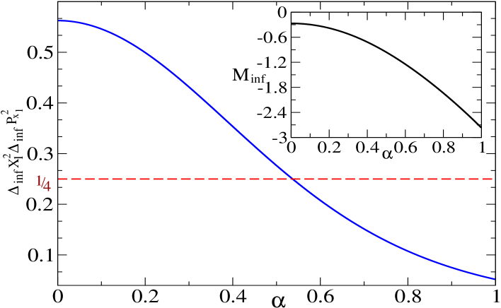
Figure 1: (Color online) The graph shows the steerability of single photon subtracted squeezed vacuum state. The solid blue curve depicts the plot of the product of inferred uncertainties, $\triangle_{\inf}X_{1}^{2}\triangle_{\inf}P_{X_{1}}^{2}$ and the red dashed line represents the lower bound of Reid’s inequality whereas the inset graph shows the plot of $M_{\inf}(X_{1}:P_{X_{1}})$ (solid black curve). It is clear that while the criteria based on the mutual uncertainty captures the steerability for any value of $\alpha$, the Reid criteria fails for $\alpha\leq\frac{1}{4}\cosh^{-1}(\frac{13}{3})\approx 0.536$.

where $\alpha$ is a squeezing parameter. Now, Alice will infer the conjugate observables ($X_{1},P_{X_{1}}$) measured at Bob’s by performing the observables ($X_{2},P_{X_{2}}$) at her side. The inferred uncertainties can directly be calculated and hence, the inferred mutual uncertainty is

$$M_{\inf}(X_{1}:P_{X_{1}})=\frac{\sqrt{3}}{2}\left(\frac{1}{\eta_{-}}+\frac{1}{\eta_{+}}\right)-(\eta_{+}+\eta_{-}),$$ (19)

where $\eta_{\pm}=\sqrt{\cosh(2\alpha)\pm\cosh(\alpha)\sinh(\alpha)}$. If $M_{\inf}(X_{1}:P_{X_{1}})<0$, then we can conclude that the state will demonstrate steering. To compare, we consider the Reid’s criteria for steering which for our case is $\triangle_{\inf}X_{1}^{2}\triangle_{\inf}P_{X_{1}}^{2}\geq 1/4$ MDsteer . For the state considered in Eq.(18), the right hand side of Reid’s inequality comes out to be

$$\triangle_{\inf}X_{1}^{2}\triangle_{\inf}P_{X_{1}}^{2}=\frac{9}{2[3\cosh(4\alpha)+5]}.$$ (20)

Now to draw comparison between two steering criteria, we plot Eqs.(19 and 20). From the Fig.(1), we find that the steerability captured by the criteria based on mutual uncertainty is more than that of Reid’s. More precisely, the criteria based on mutual uncertainty captures steerability for the whole range of $\alpha$ while the Reid’s criteria fails for $\alpha\leq\frac{1}{4}\cosh^{-1}(\frac{13}{3})\approx 0.536$.

V Discussions and conclusions

We have introduced several new quantities called as the mutual uncertainty, the conditional uncertainty and the conditional variance which may be useful in many ways to develop faithful notions in quantum information theory. In doing so, we have been able to prove many results similar to that of entropic ones such as the chain rule and the strong sub-additivity relations for the uncertainty. We have also shown that the conditional variance and the mutual uncertainty are useful to witness entanglement and quantum steering phenomenon. Specifically, as physical applications, we find that using the conditional variance, one can detect higher dimensional bipartite entangled states better than the criteria given in Ref.high_ent1 . Also, we find that the mutual uncertainty for $N$-qubit product states is exactly equal to $N-\sqrt{N}$, which provides a sufficient criteria to detect entanglement in multi-qubit pure states. Moreover, the steering criteria based on mutual uncertainty is able to detect non-Gaussian steering where Reid’s criteria MDsteer fails. In future, it may be interesting to see if these notions have other implications in quantum information science.

Acknowledgement.– AKP gratefully acknowledges the local hospitality during his visits at IOP, Bhubaneswar for the period 2014-2016, where this work has been initiated. We would like to thank Sujit Choudhary for many stimulating feedback. We greatly acknowledge the effort of the anonymous referee, which enriched the presentation as well as the quality of our work.

References

- (1) W. Heisenberg, Z. Phys. 43, 172 (1927).
- (2) E.H. Kennard, Z. Phys. 44, 326 (1927).
- (3) J.A. Wheeler and W.H. Zurek, Quantum theory and measurement, Princeton series in physics, Princeton university press, 1983.
- (4) H.P. Robertson, Phys. Rev. 35, 667 (1930).
- (5) D. Sen, Current Science 107, 203 (2014).
- (6) E. Schrödinger, Sitzungsberichte der Preussischen Akademie der Wissenschaften, Physikalisch-mathematische Klasse 14, 296 (1930).
- (7) L. Maccone and A.K. Pati, Phys. Rev. Lett. 113, 260401 (2014).
- (8) Q.-C. Song and C.-F. Qiao, arXiv: 1504.01137 (2015).
- (9) K. Wang, X. Zhan, Z. Bian, J. Li, Y. Zhang, and P. Xue, Phys. Rev. A 93, 052108 (2016).
- (10) Y. Xiao and N. Jing, Scientific Report 6, 36616 (2016).
- (11) J. Zhang, Y. Zhang, and C. Yu, arXiv: 1607.08223 (2016).
- (12) Y. Xiao, N. Jing, X. Li-Jost and S.M. Fei, Scientific Report 6, 23201 (2016).
- (13) T. Li, Y. Xiao, T. Ma, S.M. Fei, N. Jing, X. Li-Jost, and Z.-X. Wang, Scientific Report 6, 23201 (2016).
- (14) C.E. Shannon, The Bell System Technical Journal, 27, 379 (1948).
- (15) T.M. Cover and J.A. Thomas, Elements of information theory, John Wiley and Sons, Inc., New York, USA, (1991).
- (16) M.A. Nielsen and I.L. Chuang, Quantum Computation and Quantum Information, Cambridge: Cambridge University Press, (Cambridge), (2000).
- (17) M.M. Wilde, Quantum Information Theory, Cambridge University Press, (Cambridge), (2013).
- (18) H. Maassen and J.B.M. Uffink, Phys. Rev. Lett. 60, 1103 (1988).
- (19) P.J. Coles, M. Berta, M. Tomamichel, and S. Wehner, arXiv: 1511.04857 (2015).
- (20) Variance and entropy are closely related, eg., see the Refs. – Y. Huang, Phys. Rev. A 86, 024101 (2012); G. Tóth, arXiv: 1701.07461.
- (21) K. Modi, A. Brodutch, H. Cable, T. Paterek, and V. Vedral, Rev. Mod. Phys. 84, 1655 (2012).
- (22) Horodecki R., Horodecki P., Horodecki M., and Horodecki K., Rev. Mod. Phys. 81, 865 (2007).
- (23) O. Gühne and G. Tóth, Phys. Rep. 474 1 (2009).
- (24) E. Schrödinger, Proc. Cambridge Philos. Soc. 31, 553 (1935); 32, 446 (1936).
- (25) J.I. de Vicente, Quantum Inf. Comput. 7, 624 (2007).
- (26) A.K. Pati and P.K. Sahu, Phys. Lett. A 367, 177 (2007).
- (27) There exist no unique multiparticle generalization of quantum mutual information. We have considered the relative distance based one proposed in Ref.m-mutual-rela .
- (28) As an illustration of the fact that , let us consider a Harmonic oscillator Hamiltonian . Let and . With this choice, one can see the quantity can be negative. For example, if is an eigenstate of the Hamiltonian then while is positive, and hence can be negative.
- (29) H. Araki and H. Lieb, Commun. Math. Phys. 18, 160 (1970).
- (30) E.H. Lieb and M.B. Ruskai, J. Math. Phys. 14, 1938 (1973).
- (31) B. Groisman, S. Popescu, and A. Winter, Phys. Rev. A 72, 032317 (2005).
- (32) F. Herbut, J. Phys. A: Math. Gen. 37, 3535 (2004).
- (33) Sk Sazim and P. Agrawal, arXiv: 1607.05155 (2016).
- (34) B.M. Terhal, M. Horodecki, D.W. Leung, and D.P. DiVincenzo, J. Math. Phys. 43, 4286 (2002).
- (35) S. Bagchi and A.K. Pati, Phys. Rev. A 91, 042323 (2015).
- (36) H.F. Hofmann and S. Takeuchi, Phys. Rev. A 68, 032103 (2003).
- (37) O. Gühne, Phys. Rev. Lett. 92, 117903 (2004).
- (38) C. Qian, J.-L. Li, and C.-F. Qiao, Quantum Inf. Process. 17 84 (2018).
- (39) O. Gühne, P. Hyllus, O. Gittsovich, and J. Eisert, Phys. Rev. Lett. 99, 130504 (2007).
- (40) J.I. de Vicente, Phys. Rev. A 75, 052320 (2007); Erratum - Phys. Rev. A 77, 039903 (2008).
- (41) A.R. Usha Devi, R. Prabhu, and A.K. Rajagopal, Phys. Rev. Lett. 98, 060501 (2007).
- (42) S. Beigi, IEEE Xplore: in the proceedings of 2014 Iran Workshop on Communication and Information Theory (IWCIT) pp. 1-6 (2014); arXiv: 1405.2502 .
- (43) P. Agrawal, Sk Sazim, I. Chakrabarty, and A.K. Pati, Int. J. Quantum Inform. 14, 1640034 (2016).
- (44) R. Schwonnek, L. Dammeier, and R.F. Werner, Phys. Rev. Lett. 119, 170404 (2017).
- (45) J.-L. Li and C.-F. Qiao, Sci. Rep. 8, 1442 (2018).
- (46) O. Rudolph, Quantum Inf. Process. 4, 219 (2005).
- (47) K. Chen and L.-A. Wu, Quantum Inf. Comput. 3, 193 (2003).
- (48) H. Barnum, E. Knill, G. Ortiz, R. Somma, and L. Viola, Phys. Rev. Lett. 92, 107902 (2004)
- (49) L. Viola, H. Barnum, E. Knill, G. Ortiz, and R. Somma, quant-ph/0403044.
- (50) R. Somma, G. Ortiz, H. Barnum, E. Knill, and L. Viola, Phys. Rev. A 70, 042311 (2004).
- (51) S. Boixo1, L. Viola, and G. Ortiz, EPL(Europhysics Letters) 79, 40003 (2007).
- (52) Ali S.M. Hassan and P.S. Joag, Quant. Inf. and Comp. 8, 0773 (2008).
- (53) A.S.M. Hassan and P.S. Joag, Phys. Rev. A 77, 062334 (2008).
- (54) A.S.M. Hassan and P.S. Joag, Phys. Rev. A 80, 042302 (2009).
- (55) J.I. de Vicente and M. Huber, Phys. Rev. A 84, 062306 (2011).
- (56) M. Li, J. Wang, S.-M. Fei, and X. Li-Jost, Phys. Rev. A 89, 022325 (2014).
- (57) M. Li, S.-M. Fei, X. Li-Jost, and H. Fan, Phys. Rev. A 92, 062338 (2015).
- (58) R. Bhatia, Matrix analysis. Volume 169 of Graduate texts in mathematics (Springer) (1997).
- (59) A. Peres, Phys. Rev. Lett. 77, 1413 (1996); M. Horodecki, P. Horodecki, and R. Horodecki, Phys. Lett. A 223, 1 (1996).
- (60) C.H. Bennett, D.P. DiVincenzo, T. Mor, P.W. Shor, J.A. Smolin, and B.M. Terhal, Phys. Rev. Lett. 82, 5385 (1999).
- (61) The variance is invariant under the substraction of constant diagonal matrix, i.e., for observable , with and is the identity matrix. Therefore, without loss of generality one can consider traceless Hermitian operators as observables.
- (62) S. Hill and W.K. Wootters, Phys. Rev. Lett. 78, 5022 (1997); W.K. Wootters, Phys. Rev. Lett. 80, 2245 (1998).
- (63) A. Einstein, D. Podolsky, and N. Rosen, Phys. Rev. 47, 777 (1935).
- (64) M.D. Reid, Phys. Rev. A 40, 913 (1989).
- (65) H.M. Wiseman, S.J. Jones, and A.C. Doherty, Phys. Rev. Lett. 98, 140402 (2007).
- (66) S.J. Jones, H.M. Wiseman, and A.C. Doherty, Phys. Rev. A 76, 052116 (2007).
- (67) E.G. Cavalcanti and M.D. Reid, Journal of Modern Optics 54, 2373 (2007).
- (68) A.G. Maity, S. Datta, and A.S. Majumdar, Phys. Rev. A 96, 052326 (2017).
- (69) G. Sharma, C. Mukhopadhyay, S. Sazim, and A.K. Pati, arXiv: 1801.00994.
- (70) E.G. Cavalcanti, S.J. Jones, H.M. Wiseman, and M.D. Reid, Phys. Rev. A 80, 032112 (2009).
- (71) G.S. Agarwal, Quantum Optics (Cambridge University Press, Cambridge, 2013).