Transmission of charge and spin in a topological-insulator-based magnetic structure

Abstract

We discuss the effect of a magnetic thin-film ribbon at the surface of a topological insulator on the charge and spin transport due to surface electrons. If the magnetization in the magnetic ribbon is perpendicular to the surface of a topological insulator, it leads to a gap in the energy spectrum of surface electrons. As a result, the ribbon is a barrier for electrons, which leads to electrical resistance. We have calculated conductance of such a structure. The conductance reveal some oscillations with the length of the magnetized region due to the interference of transmitted and reflected waves. We have also calculated the Seebeck coefficient when electron flux is due to a temperature gradient.

PACS numbers

72.25.Dc, 72.25.Mk

I Introduction

Topological insulators (TIs) are systems which are insulators in the bulk, but their conducting properties are associated with surface (in 3-dimensional case) electronic states emerging in the gap hasan10 ; qi11 . The unique electric and magnetic properties of TIs are related mainly to robustness of the energy spectrum of surface electronic states to any perturbation which does not break the time inversion symmetry fu06 ; fu07 . This means that nonmagnetic impurities or defects do not open energy gap in the Dirac spectrum of the surface electrons. On the other hand, the effect of magnetic field or a nonzero magnetization at the surface can be crucial as they break the symmetry protection mechanism of the topological insulator liu09 ; zitko10 ; abanin11 ; cheianov12 ; rosenberg12 ; biswas10 ; zhang12 . In particular, the magnetization oriented perpendicularly to the surface of a TI opens an energy gap liu09 ; zhang12 ; henk12 ; chen10 ; wray11 , whereas the gap is absent in the case of in-plane magnetization. This behavior gives a chance to control the parameters of electron energy spectrum by variation of the magnetization orientation, that can be done, for instance, by applying a weak external magnetic field.

Another important property of surface electrons described by the Dirac Hamiltonian is the total transparency of any potential barrier for electrons incident on the barrier katsnelson . This phenomenon is known as the Klein effect. However, formation of an energy gap in the Dirac spectrum significantly changes the situation. This is because electrons can propagate only via continuous energy spectrum, and are reflected from the gap.

In this paper we discuss the possibility of using a structure with a local magnetization region on top of a TI to control transport of surface electrons. It is important that electron transport in a TI means transport of charge and spin since the electron states are spin-polarized along the direction of electron motion.

It should be noted that structures of this type attracted a lot of attention recently kong11 ; yokoyama11 ; fan14 ; mellnik14 ; semenov14 ; chang15 ; mahfouzi16 due to the possibility of an effective control of magnetization in the magnetic layer by the electric current in TI. It is related to the current-generated spin torque reversing the magnetic moments in the layer. Especially important is the spin-orbit component of the torque kurebayashi14 which is due to the current-induced spin polarization of electrons under spin-orbit interaction in the TI.

The other interesting types of a hybrid structure, which includes superconducting and magnetic layers on top of the topological insulator, have been also considered tanaka09 ; dolcini15 . In this case, one appear the Majorana excitations, which can be manipulated by the magnetization direction tanaka09 , or a possibility of controlling the phase shift in the Josephson current by the in-plane magnetic field dolcini15 .

In this paper we mostly concentrate on charge and spin transmission through the magnetized region assuming that the electric current is weak enough, so that the magnetic moments in the ribbon can be viewed as frozen. We consider the model with perpendicular magnetization. In this case the magnetization opens a gap in the electronic spectrum of TI, which creates an effective barrier for the motion of spin-polarized elecrons in TI. Thus, by controlling the magnetization orientation one can change the resistance of the structure kong11 .

II Model

We consider a system consisting of a three-dimensional (3D) topological insulator and a narrow thin-film magnetic ribbon on top of its surface. Magnetization in the ribbon is assumed to be perpendicular to the surface of TI, as shown schematically in Fig. 1. Hamiltonian which describes electrons at the surface of TI can be written in the following form:

$$\hat{H}=-iv\left(\sigma_{x}\partial_{x}+\sigma_{y}\partial_{y}\right)+m(x)\,\sigma_{z},$$ (1)

where $\sigma_{i}$ are the spin Pauli matrices, while $m(x)=gM_{z}(x)$ leads to the energy gap that is determined by the $z$-component of magnetization $M_{z}(x)$. The parameters $v/\hbar$ and $g$ are the velocity of surface electrons in TI and the coupling constant, respectively.

Figure 1: Schematic of a topological insulator with a magnetic thin-film ribbon on its surface. Magnetization ${\bf M}$ in the ribbon is perpendicular to the surface of TI.

Without any magnetic film at the surface, $m(x)=0$, the Hamiltonian (1) describes massless two-dimensional (2D) Dirac electrons at the surface of TI. The energy spectrum of such electrons has two branches, $\varepsilon_{1,2}(k)=\pm vk$. The main properties of 3D TIs are related to the fact that the low-energy electron excitations are described by massless Dirac electrons, and the spectrum is protected by the time-reversal symmetry of the system, so that any perturbation which does not break this symmetry can not open an energy gap in the Dirac spectrum hasan10 ; qi11 . As we can see from Eq. (1), Dirac electrons are spin-polarized along the wavevector ${\bf k}$, so the electric charge transmitted by Dirac electron is accompanied by the transmission of spin oriented in the direction of electron motion. One can check that any potential barrier can not stop the motion of massless Dirac electrons (Klein paradox katsnelson ).

The magnetization perpendicular to the TI surface can open the energy gap since the magnetization breaks the time-reversal invariance. As a result, electrons in TI can be effectively scattered and reflected from the barrier. We assume that the magnetic region of length $L$ is along the $x$-axis as shown in Fig. 1. Correspondingly, we can assume $m(x)$ in the following form:

$$m(x)=\left\{\begin{array}[]{cc}m_{0},&0\leq x\leq L,\\ 0,&x<0\;{\rm or}\;x>L.\end{array}\right.$$ (4)

The Schrödinger equation, $(\hat{H}-\varepsilon)\,\psi({\bf r})=0$, for the spinor components $\varphi$,$\chi$ of the wavefunction $\psi({\bf r})=e^{ik_{y}y}\psi_{k_{y}}(x)$ can be presented as

$$\left(m-\varepsilon\right)\varphi_{k_{y}}+v\left(-i\partial_{x}-ik_{y}\right)\chi_{k_{y}}=0,$$

$$v\left(-i\partial_{x}+ik_{y}\right)\varphi_{k_{y}}-\left(m+\varepsilon\right)\chi_{k_{y}}=0.$$ (5)

Since we assumed the gap in the form given by Eq. (2), these equations can be solved separately in the regions I, II and III (see Fig. 1).

III One-dimensional motion

Let us consider first the motion of electrons along the axis $x$. This corresponds to $k_{y}=0$ in equations (3). By solving these equations in the regions I ($x<0$), II ($0<x<L$) and III ($x>L$) we find (similar formulae are presented by Yokoyama yokoyama11 for a different choice of the Hamiltonian describing Bi₂Se₃ TI)

$$\psi_{k_{y}=0}(x)=\frac{e^{ik_{x}x}}{\sqrt{2}}\left(\begin{array}[]{c}1\\ 1\end{array}\right)+\frac{re^{-ik_{x}x}}{\sqrt{2}}\left(\begin{array}[]{c}1\\ -1\end{array}\right),\;x<0,$$ (10)

$$\psi_{k_{y}=0}(x)=\frac{Ae^{ik^{\prime}_{x}x}}{\sqrt{2\varepsilon(\varepsilon+m_{0})}}\left(\begin{array}[]{c}\varepsilon+m_{0}\\ \sqrt{\varepsilon^{2}-m_{0}^{2}}\end{array}\right)\hskip 36.98866pt$$ (13)

$$+\frac{Be^{-ik^{\prime}_{x}x}}{\sqrt{2\varepsilon(\varepsilon+m_{0})}}\left(\begin{array}[]{c}\varepsilon+m_{0}\\ -\sqrt{\varepsilon^{2}-m_{0}^{2}}\end{array}\right),\;0<x<L,$$ (16)

$$\psi_{k_{y}=0}(x)=\frac{te^{ik_{x}x}}{\sqrt{2}}\left(\begin{array}[]{c}1\\ 1\end{array}\right),\;x>L,\hskip 51.21504pt$$ (19)

where $r$ and $t$ are the coefficients of reflection and transmission, $A$ and $B$ are constants, $k_{x}=\varepsilon/v$, $k^{\prime}_{x}=\sqrt{\varepsilon^{2}-m_{0}^{2}}/v$, and we assumed $\varepsilon>m_{0}$.

Equation (4) represents the incoming and reflected waves with spin polarization along the direction of the electron motion. Due to external magnetization ${\bf M}$ in the region II, the waves propagating in opposite directions in this region (5) are not spin polarized in the direction of motion. If the energy of an electron is slightly above the gap, $(\varepsilon-m_{0})\ll m_{0}$, the effect of magnetization field is so strong that the electron is spin polarized along axis $z$, i.e. perpendicular to the direction of electron motion. The transmitted (outgoing) electron (6) is spin polarized along the axis $x$.

Matching the solutions (4)-(6) at the interfaces $x=0$ and $x=L$, i.e., $\psi_{k_{y}=0}(-\delta)=\psi_{k_{y}=0}(+\delta)$ and $\psi_{k_{y}=0}(L-\delta)=\psi_{k_{y}=0}(L+\delta)$, we obtain four equations for the spinor components, and finally we can find the values of all constants $r,t,A,B$ entering Eqs. (4)-(6). In particular, we find the transmission coefficient for an electron with energy $\varepsilon>m_{0}$

$$t_{k_{y}=0}=4e^{i(k^{\prime}_{x}-k_{x})L}\sqrt{\varepsilon^{2}-m_{0}^{2}}\left[\left(\sqrt{\varepsilon+m_{0}}+\sqrt{\varepsilon-m_{0}}\right)^{2}\right.$$

$$\left.-e^{2ik^{\prime}_{x}L}\left(\sqrt{\varepsilon+m_{0}}-\sqrt{\varepsilon-m_{0}}\right)^{2}\right]^{-1}.\hskip 14.22636pt$$ (20)

From this equation follows that the probability of transmission through the ”magnetization barrier”, $T_{k_{y}=0}=|t_{k_{y}=0}|^{2}$, can go to zero if the electron energy is close to the value of the gap, $(\varepsilon-m_{0})\ll m_{0}$ and $L\to\infty$.

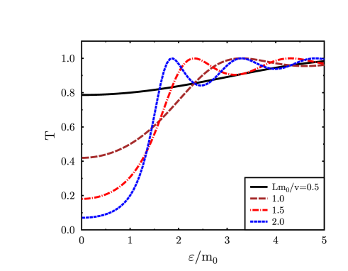
Figure 2: Transmission probability $T_{k_{y}=0}$ as a function of energy for different length of magnetization region. Electron is moving along axis $x$.

Indeed, in the limit of $(\varepsilon-m_{0})\ll m_{0}$ from Eq. (7) follows

$$T_{k_{y}=0}\simeq\frac{4\,(\varepsilon-m_{0})}{m_{0}(1-\cos 2k^{\prime}_{x}L)+2(\varepsilon-m_{0})(1+\cos 2k^{\prime}_{x}L)}\,,\hskip 5.69046pt$$ (21)

which means that the transmission probabilty $T_{k_{y}=0}$ is oscillating with the length $L$. These oscillations are due to the interference of transmitted and reflected waves in the magnetized region. If $k^{\prime}_{x}L$ is not very close to $n\pi$ ($n$ is integer), then we obtain $T_{k_{y}=0}=0$ but at the points $k^{\prime}_{x}L=n\pi$ we get $T_{k_{y}=0}=1$. Since $k^{\prime}_{x}=\sqrt{\varepsilon^{2}-m_{0}^{2}}/v$, for $(\varepsilon-m_{0})\ll m_{0}$ and small enough $L\ll v/\sqrt{2m_{0}(\varepsilon-m_{0})}$ we also obtain full transparency of the magnetic barrier, $T_{k_{y}=0}\simeq 1$. It should be also mentioned that when $T_{k_{y}=0}=0$, the constants $A$ and $B$ in Eq. (5) do not vanish, which indicates that an electron coming from the region I can partially penetrate into the region II, but it does not go through the outer interface $x=L$. In the case of large electron energy, $\varepsilon\gg m_{0}$, we find from Eq. (7) that $T_{k_{y}=0}\simeq 1$, like in the case of TI without any magnetic barrier.

The electrons with energies $\varepsilon<m_{0}$ can penetrate through the gap by tunneling. In this case, the wavefunction in region II has the following form

$$\psi_{k_{y}=0}(x)=\frac{Ae^{\kappa x}}{\sqrt{2m_{0}(\varepsilon+m_{0})}}\left(\begin{array}[]{c}\varepsilon+m_{0}\\ -i\sqrt{m_{0}^{2}-\varepsilon^{2}}\end{array}\right)$$ (24)

$$+\frac{Be^{-\kappa x}}{\sqrt{2m_{0}(\varepsilon+m_{0})}}\left(\begin{array}[]{c}\varepsilon+m_{0}\\ i\sqrt{m_{0}^{2}-\varepsilon^{2}}\end{array}\right),\;0<x<L,$$ (27)

where $\kappa=\sqrt{m_{0}^{2}-\varepsilon^{2}}/v$. Hence, calculating the transmission coefficient like before we find for $0<\varepsilon<m_{0}$

$$t_{k_{y}=0}=-4ie^{(\kappa-ik_{x})L}\sqrt{m_{0}^{2}-\varepsilon^{2}}$$

$$\times\left[\left(\sqrt{m_{0}+\varepsilon}-i\sqrt{m_{0}-\varepsilon}\right)^{2}\right.$$

$$\left.-e^{2\kappa L}\left(\sqrt{m_{0}+\varepsilon}+i\sqrt{m_{0}-\varepsilon}\right)^{2}\right]^{-1}.$$ (28)

Using this expression (10) we can find that for $\varepsilon\ll m_{0}$ the transmission probability has a simple form

$$T_{k_{y}=0}=\frac{2}{1+\cosh(2\kappa L)}\;,$$ (29)

and in the limit of $\kappa L\to 0$ we get $T_{k_{y}=0}=1$.

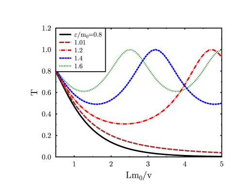
Figure 3: Transmission probability $T_{k_{y}=0}$ as a function of length $L$ of the magnetized region for different values of electron energy. Electrons are moving along the axis $x$.

The dependence of transmission probabilty $T_{k_{y}=0}$ on the electron energy $\varepsilon$ and on the length $L$ are presented in Figs. 2 and 3, respectively. Here we used the dimensionless energy $\varepsilon/m_{0}$ and length $Lm_{0}/v$. If we take $m_{0}=100$ meV and $v=10^{-8}$ eV$\cdot$cm, we obtain the value of length unit $v/m_{0}=1$ nm.

IV Two-dimensional motion of electrons

Let us consider first overbarrier transmission of electrons. Taking into account a nonzero value of $k_{y}$ for electrons incoming at a certain angle to the surface, we write the solution of Eqs. (3) for the wavefunction in the regions I, II, and III as (we omit the common multiplier $e^{ik_{y}y}$)

$$\psi_{\bf k}(x)=\frac{e^{ik_{x}x}}{\sqrt{2}}\left(\begin{array}[]{c}1\\ k_{+}/k\end{array}\right)+\frac{re^{-ik_{x}x}}{\sqrt{2}}\left(\begin{array}[]{c}1\\ -k_{-}/k\end{array}\right),\;x<0,\hskip 14.22636pt$$ (34)

$$\psi_{\bf k}(x)=\frac{Ae^{ik^{\prime}_{x}x}}{\sqrt{2\varepsilon(\varepsilon+m_{0})}}\left(\begin{array}[]{c}\varepsilon+m_{0}\\ vk^{\prime}_{+}\end{array}\right)\hskip 56.9055pt$$ (37)

$$+\frac{Be^{-ik^{\prime}_{x}x}}{\sqrt{2\varepsilon(\varepsilon+m_{0})}}\left(\begin{array}[]{c}\varepsilon+m_{0}\\ -vk^{\prime}_{-}\end{array}\right),\;0<x<L,$$ (40)

$$\psi_{\bf k}(x)=\frac{t\,e^{ik_{x}x}}{\sqrt{2}}\left(\begin{array}[]{c}1\\ k_{+}/k\end{array}\right),\;x>L,\hskip 51.21504pt$$ (43)

where we denote $k_{\pm}=k_{x}\pm ik_{y}$, $k^{\prime}_{\pm}=k^{\prime}_{x}\pm ik_{y}$, and $k^{\prime}_{x}=(\varepsilon^{2}-m_{0}^{2}-v^{2}k_{y}^{2})^{1/2}/v$. Here we take into account that the $k_{y}$ component of vector ${\bf k}$ is conserved when the electron is transmitted through the interface. This is due to the translational invariance along $y$. Note that here we use vector ${\bf k}$ being the wavevector of incoming wave as a quantum number to label scattering states, which are the eigenstates of Schrödinger equation with Hamiltonian (1).

After matching Eqs. (12) to (14) at $x=0$ and $x=L$ one can obtain the following expression for transmission coefficient depending on the direction of vector ${\bf k}$ for $\varepsilon>(m_{0}^{2}+v^{2}k_{y}^{2})^{1/2}$

$$t({\bf k})=2vk^{\prime}_{x}\,e^{i(k^{\prime}_{x}-k_{x})L}(1+k/k_{+})\,(\varepsilon+m_{0})\hskip 22.76228pt$$

$$\times\Big{[}\Big{(}\varepsilon+m_{0}+\frac{\varepsilon k^{\prime}_{+}}{k_{-}}\Big{)}\Big{(}\varepsilon+m_{0}+\frac{\varepsilon k^{\prime}_{-}}{k_{+}}\Big{)}-e^{2ik^{\prime}_{x}L}$$

$$\times\Big{(}\varepsilon+m_{0}-\frac{\varepsilon k^{\prime}_{+}}{k_{+}}\Big{)}\Big{(}\varepsilon+m_{0}-\frac{\varepsilon k^{\prime}_{-}}{k_{-}}\Big{)}\Big{]}^{-1}.$$ (44)

One can check that electrons incident on the interface at a nonzero angle $\phi=\tan^{-1}(k_{y}/k_{x})$ are not transferred so easily as those with $\phi=0$.

One can also consider the subbarrier transmission of electrons. In this case the electrons are tunneled through the gap, and instead of Eq. (13) we get

$$\psi_{\kappa,k_{y}}(x)=\frac{1}{\sqrt{2[m_{0}(\varepsilon+m_{0})+v^{2}k_{y}(k_{y}-\kappa)]}}\hskip 28.45274pt$$

$$\times\left[Ae^{\kappa x}\left(\begin{array}[]{c}\varepsilon+m_{0}\\ -iv(\kappa-k_{y})\end{array}\right)+Be^{-\kappa x}\left(\begin{array}[]{c}\varepsilon+m_{0}\\ iv(\kappa+k_{y})\end{array}\right)\right],$$ (49)

$$0<x<L,\hskip 14.22636pt$$ (50)

whereas for $x<0$ and $x>L$ we can use again Eqs. (12) and (14). Here we denote $\kappa=(m_{0}^{2}+v^{2}k_{y}^{2}-\varepsilon^{2})^{1/2}/v$.

Then for the transmission coefficient at $0<\varepsilon<(m_{0}^{2}+v^{2}k_{y}^{2})^{1/2}$ we obtain

$$t({\bf k})=\Big{(}1+\frac{k_{+}}{k_{-}}\Big{)}\,\sqrt{m_{0}\left(\varepsilon+m_{0}\right)+v^{2}k_{y}(k_{y}-\kappa)}$$

$$\times\left(\varepsilon+m_{0}-iv(\kappa+k_{y})\frac{k_{+}}{k}\right)\hskip 28.45274pt$$

$$\times\left[\left(\varepsilon+m_{0}-iv(\kappa+k_{y})\frac{k}{k_{-}}\right)\hskip 28.45274pt\right.$$

$$\left.\times\left(\varepsilon+m_{0}-iv(\kappa+k_{y})\frac{k_{+}}{k}\right)\hskip 28.45274pt\right.$$

$$\left.-e^{2\kappa L}\,\left(\varepsilon+m_{0}+iv(\kappa+k_{y})\frac{k}{k_{-}}\right)\hskip 28.45274pt\right.$$

$$\left.\times\left(\varepsilon+m_{0}+iv(\kappa-k_{y})\frac{k_{+}}{k}\right)\right]^{-1}.$$ (51)

The results (15) and (17) can be used for the calculation of various transport properties of TI/magnetic layer structures. Here we present the calculation of conductance and thermoelectricity.

V Conductance

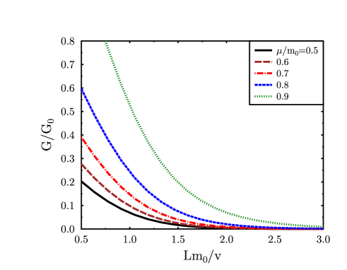
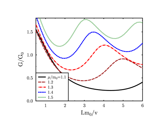
Figure 4: Electrical conductance as a function of length $L$ of the magnetized region for indicated values of the Fermi level $\mu$. The character of curves is different in the tunneling regime, $\mu<m_{0}$ and at the overbarrier transmission, $\mu>m_{0}$.

Now we calculate the conductance of the structure assuming that the magnetic nanoribbon is a unique barrier for the motion of electrons along the surface (usual impurities are fully transparent). Then we take chemical potential $\mu$ on the right side (region III) and $\mu+eU$ on the left side (region I). This corresponds to the electron flux from left to right (see Fig. 1) under external voltage $U$.

The electric current across the magnetic region reads

$$j=\frac{ev}{\hbar}{\sum}^{\prime}_{\bf k}\frac{k_{x}}{k}|t({\bf k})|^{2}\big{[}\theta(\mu+eU-\varepsilon_{1k})-\theta(\mu-\varepsilon_{1k})\big{]},\hskip 11.38092pt$$ (52)

where $vk_{x}/\hbar k$ is the $x$-component of electron velocity in region III, $\varepsilon_{1k}=vk$ is the energy spectrum of electrons in region III with energy $\varepsilon>0$, and $\theta(z)$ is the Heaviside’s function. The sum over ${\bf k}$ is restricted by $k_{x}>0$.

The results of numerical calculation of the electric conductance $G=jL/U$ are presented in Fig. 4, where we denote $G_{0}=e^{2}/\hbar$. As we see, for $\mu>m_{0}$ the conductance is also oscillating with $L$, similarly to the transmission probability $T_{k_{y}=0}$. This is because the main contribution to the current is related to electrons incoming with the small value of $k_{y}$, i.e., perpendicular to the interface.

VI Thermoelectricity

Figure 5: Linear response thermoelectric coefficient $\beta$ as a function of $L$ for different values of the chemical potential $\mu$.

Using the transmission coefficient (15) and (17) in the region of overbarrier motion and tunneling, one can also calculate the electric current generated by a temperature gradient (Seebeck effect). We assume that the temperature of TI in the regions I and III is $T_{1,2}=T\pm\Delta T/2$, respectively. The thermoelectric current can be then written in the form

$$j_{T}=\frac{ev}{\hbar}{\sum}^{\prime}_{\bf k}\frac{k_{x}}{k}\,|t({\bf k})|^{2}\big{[}f_{1}(\varepsilon_{1k}-\mu)-f_{2}(\varepsilon_{1k}-\mu)\big{]},\hskip 11.38092pt$$ (53)

where $f_{1,2}(z)=[\exp(z/k_{B}T_{1,2})+1]^{-1}$ are the Fermi-Dirac distribution functions in the region I and III, and we assume $\Delta T\ll\mu/k_{B}$ so that the thermoelectricity is due to electrons in the upper energy band $\varepsilon_{1k}$.

The results of numerical calculation of the linear response thermoelectric coefficient $\beta$ defined as $\beta\equiv GS=j_{T}L/m_{0}T$, where $S$ is the Seebeck coefficient and we denote $\beta_{0}=ek_{B}/\hbar$, are presented in Fig. 5. Like the electrical conductance, the thermoelectric coefficient $\beta$ reveals some oscillations with increasing magnetic region length $L$. As we see, the dependence of $\beta$ on $L$ is very similar to the dependence of conductance $G(L)$ because in both cases the main effect is mostly related to the dependence of transmission coefficion on the length $L$.

VII Application of the Dirac model to ${\rm Bi}_{2}{\rm Se}_{3}$ topological insulator and the spin torque

The standard model of ${\rm Bi}_{2}{\rm Se}_{3}$ topological insulator uses the following Hamiltonian (without magnetization term)

$$H_{0}=-iv(\sigma_{x}\partial_{y}-\sigma_{y}\partial_{x}),$$ (54)

which differs from the Dirac model in Eq. (1). However, by using unitary transformation $U={\rm diag}(1,i)$ the Dirac Hamiltonian $H_{0}=-iv\mbox{$\bm{\sigma}$}\cdot\mbox{$\bm{\nabla}$}$ transforms into (20). It means just a different choice of the phase in basis functions in ”different” models. The corresponding transformation of Pauli matrices is $U^{\dagger}\sigma_{x}U=-\sigma_{y}$, $U^{\dagger}\sigma_{y}U=\sigma_{x}$ and $U^{\dagger}\sigma_{z}U=\sigma_{z}$. Thus, the Dirac model with magnetization (1) describes the Bi₂Te₃ TI with magnetization along the same axis $z$. The spin polarization of electrons along the direction of motion (helicity) in the Dirac model corresponds to the polarization perpendicular to the direction of electron motion in Bi₂Te₃ TI. This allows us to use all the results of calculation of transmission of electrons through the magnetized region in Bi₂Te₃ with the standard Dirac model (1).

The problem of spin torque needs special consideration, which is not in the scope of this paper, and we restrict ourselves by briefly discussing the main points. The total spin transfer torque (STT) acting on the moments in the magnetized regions can be calculated as a difference of incoming and outgoing spin currents. Since the spin currents in incoming and reflected waves have the same sign, and there is a relation between reflection $R$ and transmission $T$ probability, $T+R=1$, one can find the following expression for STT

$$\mathcal{T}_{STT}=v{\sum}^{\prime}_{\bf k}\frac{k_{x}}{k}\,\big{(}1-|t({\bf k})|^{2}\big{)}\big{[}\theta(\mu+eU-\varepsilon_{1k})$$

$$-\theta(\mu-\varepsilon_{1k})\big{]}.$$ (55)

In the case of Bi₂Te₃ TI the spin polarization of current is along $-y$. Thus, the STT component of torque is also along $-y$ leading to current-induced deviation of magnetic moments from perpendicular. The maximum of STT is for $|t({\bf k})|^{2}=0$ (full reflection), whereas at a full transparency, $|t({\bf k})|^{2}=1$, STT is zero.

Another component of the torque, namely, the spin-orbit torque (SOT) is nonzero due to the spin-polarized electrons in TI. Indeed, the nonequilibrium current along axis $x$ is associated with the prevailing number of electrons with spin in $-y$ direction, which results in a nonequilibrium magnetization $\mathcal{M}_{y}$ of the electron gas. In its turn, it leads to the generation of SOT acting at the magnetic moments as $\mbox{$\bm{\mathcal{T}}$}_{SOT}\sim{\bf M}\times\mbox{$\bm{\mathcal{M}}$}$, i.e. along $x$.

VIII Conclusions

We calculated the conductance and thermoelectric coefficient of a topological-insulator-based structure consisting of a TI and a thin magnetic ribbon on its surface. In fact, these parameters characterize transport properties of the region II since transport in the regions I and III is purely ballistic.

It should be noted that we did not take into account the possibility of scattering from impurities in the region II. In contrast to the transport through regions I and III, transport in the region II depends on the presence of potential scatterers, which appears due to the gap. However, we can neglect this effect as we consider narrow magnetic ribbon, i.e., when $L\ll\ell$, where $\ell$ is the mean free path of electrons in the region $0<x<L$.

It is also interesting to analyze the problem of spin transmission through the region under the magnetic ribbon in the Dirac model of TI. Generally, the electron spin is not conserved when an electron traverses the magnetic region, contrary to the electric charge which has to be conserved. As we see from Eqs. (4) and (5), spin of an electron changes its orientation when it passes through the interface $x=0$, whereas reflected electrons have spin orientation opposite to the spin of incoming electrons. Thus, the flux of electrons reflected from the interface $x=0$ is associated with the spin current $J_{x}$ (spin along $x$) in the same direction as the spin flux of incoming electrons. This indicates that the spin current in region I is enhanced with increasing reflection coefficient $R=|r|^{2}$. In the limit of $R\to 1$ we get the net spin current generator in the absence of charge current. In turn, the spin current in the region III flows in the same direction as the particle (electron) flux, which is proportional to the transmission coefficient $T=|t|^{2}$. Therefore, the spin current passing through the structure is not conserved, due to the spin torque exerted on magnetic moments in the region II. The maximum spin torque corresponds to the limit of $T=0$, i.e., to the limit of total reflection of electrons.

- (1) M. Z. Hasan and C. L. Kane, Rev. Mod. Phys. 82, 3045 (2010),
- (2) X. L. Qi and S. C. Zhang, Rev. Mod. Phys. 83, 1057 (2011).
- (3) L. Fu and C. L. Kane, Phys. Rev. B 74, 195312 (2006).
- (4) L. Fu and C. L. Kane, Phys. Rev. B 76, 045302 (2007),
- (5) Q. Liu, C. X. Liu, C. Xu, X. L. Qi, and S. C. Zhang, Phys. Rev. Lett. 102, 156603 (2009).
- (6) R. itko, Phys. Rev. B 81, 241414 (2010).
- (7) D. A. Abanin and D. A. Pesin, Phys. Rev. Lett. 106, 136802 (2011).
- (8) V. Cheianov, M. Szyniszewski, E. Burovski, Yu. Sherkunov, and V. Fal’ko, Phys. Rev. B 86, 054424 (2012).
- (9) G. Rosenberg and M. Franz, Phys. Rev. B 85, 195119 (2012).
- (10) R. R. Biswas and A. V. Balatsky, Phys. Rev. B 81, 233405 (2010).
- (11) D. Zhang, A. Richardella, D. W. Rench, S. Y. Xu, A. Kandala, T. C. Flanagan, H. Beidenkopf, A. L. Yeats, B. B. Buckley, P. V. Klimov, D. D. Awschalom, A. Yazdani, P. Schiffer, M. Z. Hasan, and N. Samarth, Phys. Rev. B 86, 205127 (2012).
- (12) J. Henk, A. Ernst, S. V. Eremeev, E. V. Chulkov, I. V. Maznichenko, and I. Mertig, Phys. Rev. Lett. 108, 206801 (2012).
- (13) Y. L. Chen, J.-H. Chu, J. G. Analytis, Z. K. Liu, K. Igarashi, H.-H. Kuo, X. L. Qi, S. K. Mo, R. G. Moore, D. H. Lu, M. Hashimoto, T. Sasagawa, S. C. Zhang, I. R. Fisher, Z. Hussain, Z. X. Shen, Science 329, 659 (2010).
- (14) L. A. Wray, S.-Y. Xu, Y. Xia, D. Hsieh, A. V. Fedorov, Y. S. Hor, R. J. Cava, A. Bansil, H. Lin and M. Z. Hasan, Nature Phys. 7, 32 (2011).
- (15) M. I. Katsnelson, Graphene: Carbon in Two Dimensions, Chap. 4 (Cambridge Univ. Press, 2012).
- (16) B. D. Kong, Y. G. Semenov, C. M. Krowne, and K. W. Kim, Appl. Phys. Lett. 98, 243112 (2011).
- (17) T. Yokoyama, Phys. Rev. B 84, 113407 (2011).
- (18) Y. Fan, P. Upadhyaya, X. Kou, M. Lang, S. Takei, Z. Wang, J. Tang, L. He, L.-T. Chang, M. Montazeri, G. Yu, W. Jiang, T. Nie, R. N. Schwartz, Y. Tserkovniak, and K. L. Wang, Nature Mat. 13, 699 (2014).
- (19) A. R. Mellnik, J. S. Lee, A. Richardella, J. L. Grab, P. J. Mintun, M. H. Fischer, A. Vaezi, A. Manchon, E.-A. Kim, N. Samarth, and D. C. Ralph, Nature 511, 449 (2014).
- (20) Y. G. Semenov, X. Duan, and K. W. Kim, Phys. Rev. B 89, 201405(R) (2014).
- (21) P.-H. Chang, T. Markussen, S. Smidstrup, K. Stokbro, and B. K. Nikolić, Phys. Rev. B 92, 201406(R) (2015).
- (22) F. Mahfouzi, B. K. Nikolić, and N. Kioussis, Phys. Rev. B 93, 115419 (2016).
- (23) H. Kurebayashi, J. Sinova, D. Fang, A. C. Irvine, T. D. Skinner, J. Wunderlich, V. Novaák, R. P. Gallagher, E. K. Vehstedt, L. P. Zárbo, K. Výborný, A. J. Ferguson, and T. Jungwirth, Nature Nanotechnol. 9, 211 (2014).
- (24) Y. Tanaka, T. Yokoyama, and N. Nagaosa, Phys. Rev. Lett. 103, 107002 (2009).
- (25) F. Dolcini, M. Houzet, and J. S. Meyer, Phys. Rec. B 92, 035428 (2015).