Efficient high-resolution RF pulse design applied to simultaneous multi-slice excitation

Abstract

RF pulse design via optimal control is typically based on gradient and quasi-Newton approaches and therefore suffers from slow convergence. We present a flexible and highly efficient method that uses exact second-order information within a globally convergent trust-region CG-Newton method to yield an improved convergence rate. The approach is applied to the design of RF pulses for single- and simultaneous multi-slice (SMS) excitation and validated using phantom and in-vivo experiments on a $3\text{\,}\mathrm{T}$ scanner using a modified gradient echo sequence.

Keywords pulse design, optimal control, second-order methods, simultaneous multi-slice excitation

1 Introduction

For many applications in MRI there is still demand for the optimization of selective RF excitation, e.g., for simultaneous multi-slice excitation [30, 49], UTE imaging [8], or velocity selective excitation [15]. To achieve a well-defined slice profile at high field strength while meeting B₁ peak amplitude limitations is a challenge for RF pulse design and becomes especially critical for quantitative methods. Correspondingly, many approaches for general pulse design have been proposed in the literature. RF pulses with low flip angles can be designed using the small tip angle simplification [37], which makes use of an approximation of the Bloch equation to compute a pulse via the Fourier transform of the desired slice profile. However, this simplification breaks down for large flip angles. The resulting excitation error for large flip angle pulses can be reduced by applying the Shinnar–Le Roux (SLR) technique [38] or optimization methods, e.g., simulated annealing, evolutionary approaches or optimal control [45, 54, 26, 12, 56, 29, 51]. The SLR method is based on the hard pulse approximation and a transformation of the excitation problem, allowing to solve the excitation problem recursively by applying fast filter design algorithms such as the Parks–McClellan algorithm [38]. Originally, this approach only covered special pulses such as $90\mathrm{°}$ and $180\mathrm{°}$ excitation or refocusing, but Lee [31] generalized this approach to arbitrary flip angles with an exact parameter relation. Despite its limitations due to neglected relaxation terms and sensitivity to B₁ inhomogeneities, it found widespread use (see, e.g., [31, 3, 21, 32]) and is considered to be the gold standard for large tip angle pulse design. An alternative approach is based on optimizing a suitable functional; see, e.g., [50, 56, 38, 19, 7]. In particular, optimal control (OC) approaches involve the solution of the Bloch equation describing the evolution of the magnetization vector in an exterior magnetic field [12, 27, 46, 5, 29, 20, 56, 51]. They often lead to better excitation profiles due to a more accurate design model and are increasingly used in MRI, for instance, to perform multidimensional and multichannel RF design [56, 20], robust 2D spatial selective pulses [51] and saturation contrast [29]. In addition, arbitrary flip angles and target slice profiles, as well as inclusion of additional physical effects such as, e.g., relaxation can be handled. However, so far OC approaches are limited by the computational effort and require a proper modeling of the objective. In particular, standard gradient-based approaches suffer from slow convergence, imposing significant limitations on the accuracy of the obtained slice profiles. On the other hand, Newton methods show a locally quadratic convergence, but require second-order information which in general is expensive to compute [1]. Approximating the Hessian using finite differences causes loss of quadratic convergence due to the lack of exact second-order information and typically requires significantly more iterations. Superlinear convergence can be obtained using quasi-Newton methods based on exact gradients [14], although their performance can be sensitive to implementation details. The purpose of this work is to demonstrate that for the OC approach to pulse design, it is in fact possible to use exact second-order information while avoiding the need of computing the full Hessian, yielding a highly efficient numerical method for the optimal control of the full time-dependent Bloch equation. In contrast to [1] (which uses black-box optimization method and symbolically calculated Hessians based on an effective-matrix approximation of the Bloch equation), we propose a matrix-free Newton–Krylov method [28] using first- and second-order derivatives based on the adjoint calculus [24] together with a trust-region globalization [48]; for details we refer to Section 2.2. Recently, similar matrix-free Newton–Krylov approaches with line search globalization were presented for optimal control of quantum systems in the context of NMR pulse sequence design [11, 10]. In comparison, the proposed trust-region framework significantly reduces the computational effort, particularly for the initial steps far away from the optimum. The effectiveness of the proposed method is demonstrated for the design of pulses for single and simultaneous multi-slice excitation (SMS).

SMS excitation is increasingly used to accelerate imaging experiments [30, 36, 17, 49]. Conventional design approaches, based on a superposition of phase-shifted sub-pulses [33] or sinusoidal modulation [30], typically result in a linear scaling of the B₁ peak amplitude, a quadratic peak power and a linear increase in the overall RF power [35, 2]. The required maximal B₁ peak amplitude of conventional multi-slice pulses therefore easily exceeds the transmit voltage of the RF amplifier. In this case, clipping will occur, while rescaling will decrease and limit the maximal flip angle of such a pulse. On the other hand, restrictions of the specific absorption rate limit the total (integrated) B₁ power and therefore the maximal number of slices as well as the pulse duration and flip angle. The increase of B₁ power can be addressed by the Power Independent of Number of Slices (PINS) technique [35], which was extended to the kT-PINS method [43] to account for B₁ inhomogeneities. This approach leads to a nearly slice-independent power requirement, but the periodicity of the resulting excitation restricts the slice orientation and positioning. Furthermore, the slice profile accuracy is reduced [17], and a limited ratio between slice thickness and slice distance may further restrict possible applications. The combination of PINS with regular multi-band pulses was shown to reduce the overall RF power by up to $50\text{\,}\mathrm{\char 37\relax}$ (MultiPINS [16]) and was applied to refocusing pulses in a multi-band RARE sequence with 13 slices [18].

A different way to reduce the maximum B₁ amplitude is to increase the pulse length; however, this stretching increases the minimal echo and repetition times and decreases the RF bandwidth, thus reducing the slice profile accuracy [2]. Applying variable rate selective excitation [13, 41] avoids this problem but leads to an increased sensitivity to slice profile degradations at off-resonance frequencies. In addition, they require specific sequence alterations, e.g., variable slice gradients or gradient blips. Instead of using the same phase for all sub-slices, the peak power can be reduced by changing the uniform phase schedule to a different phase for each individual slice [53]. Alternative approaches[57, 44] using phase-matched excitation and refocusing pairs show that a nonlinear phase pattern can be corrected by a subsequent refocusing pulse. Another way to reduce the power deposition and SAR of SMS pulses is to combine them with parallel transmission [25]. This allows to capitalize transmit sensitivities in the pulse design and leads to a more uniform excitation with an increased power efficiency [55, 39]. Recently, Guerin et al. [22] demonstrated that it is possible to explicitly control both global and local SAR as well as the peak power using a spokes-SMS-pTx pulse design.

The focus of this work, however, is on single channel imaging, where we apply our OC-based pulse design for efficient SMS pulse optimization using a direct description of the desired magnetization pattern. Its flexible formulation allows a trade-off between the slice profile accuracy and the required pulse power and is well suited for the reduction of power and amplitude requirements of such pulses, even for a large number of slices or large flip angles or in presence of relaxation. The efficient implementation of the proposed method allows to optimize for SMS pulses with a high spatial resolution to achieve accurate excitation profiles. The RF pulses are designed to achieve a uniform effective echo time and phase for each slice and use a constant slice-selective gradient, allowing to insert the RF pulse into existing sequences and opening up a wide range of applications.

2 Theory

This section is concerned with the description of the optimal control approach to RF pulse design as well as of the proposed numerical solution approach.

2.1 Optimal control framework

Our OC approach is based on the full time-dependent Bloch equation, which describes the temporal evolution of the ensemble magnetization vector ${M}(t)=({M_{x}}(t),{M_{y}}(t),{M_{z}}(t))^{T}$ due to a transient external magnetic field ${B}(t)$ as the solution of the ordinary differential equation (ODE)

(1) $$\left\{\begin{aligned} \dot{{M}}(t)&=\gamma{B}(t)\times{M}(t)+{R}({M}(t)),\qquad t>0,\\ {M}(0)&={M^{0}},\end{aligned}\right.$$

where $\gamma$ is the gyromagnetic ratio, ${M^{0}}$ is the initial magnetization and

(2) $${R(M}(t))=(-{M_{x}}(t)/T_{2},-{M_{y}}(t)/T_{2},-({M_{z}}(t)-M_{0})/T_{1})^{T}$$

denotes the relaxation term with relaxation times $T_{1},T_{2}$ and the equilibrium magnetization $M_{0}$. To encode spatial information in MR imaging, the external magnetic field ${B}$ (and thus the magnetization vector) depends on the slice direction $z$, hence the Bloch equation can be considered as a parametrized family of three-dimensional ODEs. In the on-resonance case and ignoring spatial field inhomogeneities, the Bloch equation can be expressed in the rotating frame as

(3) $$\left\{\begin{aligned} {\dot{M}}(t;z)&={A}({u}(t);z){M}(t;z)+{b}(z),\qquad t>0,\\ {M}(0;z)&={M^{0}}(z),\end{aligned}\right.$$

where the control ${u}(t)=({u_{x}}(t),{u_{y}}(t))$ describes the RF pulse,

(4) $${A}({u};z)=\begin{pmatrix}-\frac{1}{T_{2}}&\gamma{G_{z}}(t)z&\gamma{u_{y}}(t)B_{1}\\ -\gamma{G_{z}}(t)z&-\frac{1}{T_{2}}&\gamma{u_{x}}(t)B_{1}\\ -\gamma{u_{y}}(t)B_{1}&-\gamma{u_{x}}(t)B_{1}&-\frac{1}{T_{1}}\end{pmatrix},\qquad{b}(z)=\begin{pmatrix}0\\ 0\\ \frac{{M_{0}}}{T_{1}}\end{pmatrix},$$

and $G_{z}$ is the slice-selective gradient; see, e. g., [34, Chapter 6.1].

The OC approach consists in computing for given initial magnetization ${M^{0}}(z)$ the RF pulse ${u}(t)$, $t\in[0,T_{u}]$, that minimizes the squared error at read-out time $T>T_{u}$ between the corresponding solution ${M}(T;z)$ of (3) and a prescribed slice profile ${M_{d}}(z)$ for all $z\in[-a,a]$ together with a quadratic cost term modeling the SAR of the pulse, i.e., solving

(5) $$\min\limits_{({u},{M})\text{ satisfying \eqref{eq:bloch_rot}}}\quad J({M},{u})=\frac{1}{2}\int_{-a}^{a}|{M}(T;z)-{M_{d}}(z)|_{2}^{2}\,dz+\frac{\alpha}{2}\int_{0}^{T_{u}}|{u}(t)|_{2}^{2}\,dt.$$

The parameter $\alpha>0$ controls the trade-off between the competing goals of slice profile attainment and SAR reduction.

2.2 Adjoint approach

The standard gradient method for solving (5) consists of computing for given ${u}^{k}$ the gradient ${g}({u}^{k})$ of $j({u}):=J({M}({u}),{u})$ and setting ${u}^{k+1}={u}^{k}-s^{k}{g}({u}^{k})$ for some suitable step length $s^{k}$. The gradient can be calculated efficiently using the adjoint method, which in this case yields

(6) $${g}({u}^{k})(t) =\alpha{u}(t)+\gamma B_{1}\begin{pmatrix}\int_{-a}^{a}{M_{z}}(t;z){P_{y}}(t;z)-{M_{y}}(t;z){P_{z}}(t;z)\,dz\\[2.15277pt] \int_{-a}^{a}{M_{z}}(t;z){P_{x}}(t;z)-{M_{x}}(t;z){P_{z}}(t;z)\,dz\end{pmatrix}$$

$$=:\alpha{u}(t)+\begin{pmatrix}\int_{-a}^{a}{M}(t;z){A_{1}}{P}(t;z)\,dz\\[2.15277pt] \int_{-a}^{a}{M}(t;z){A_{2}}{P}(t;z)\,dz\end{pmatrix},\qquad 0\leq t\leq T_{u},$$

where ${M}$ is the solution to (3) for ${u}={u}^{k}$ and $0<t\leq T$, ${P}$ is the solution to the adjoint (backward in time) equation

(7) $$\left\{\begin{aligned} -\dot{{P}}(t;z)&={A}({u}(t);z)^{T}{P}(t;z),\qquad 0\leq t<T,\\ {P}(T;z)&={M}(T;z)-{M_{d}}(z),\end{aligned}\right.$$

and for the sake of brevity, we have set

(8) $${A_{1}}:=\gamma B_{1}\begin{pmatrix}0&0&0\\ 0&0&-1\\ 0&1&0\end{pmatrix},\qquad{A_{2}}:=\gamma B_{1}\begin{pmatrix}0&0&-1\\ 0&0&0\\ 1&0&0\end{pmatrix}.$$

However, this method requires a line search to converge and usually suffers from slow convergence close to a minimizer. This is not the case for Newton’s method (which is a second-order method and converges locally quadratically), where one additionally computes the Hessian ${H}({u}^{k})$ of $j$ at $u^{k}$, solves for $\delta{u}$ in

(9) $${H}({u}^{k})\delta{u}=-{g}({u}^{k}),$$

and sets ${u}^{k+1}={u}^{k}+\delta{u}$. While the full Hessian ${H}({u}^{k})$ is very expensive to compute in practice, solving (9) using a Krylov method such as conjugate gradients (CG) only requires computing the Hessian action ${H}({u}^{k}){h}$ for a given direction ${h}$ per iteration; see, e.g., [28]. The crucial observation in our approach is that the adjoint method allows computing this action exactly (e.g., without employing finite difference approximations) and without knowledge of the full Hessian. Since Krylov methods usually converge within very few iterations, this so-called “matrix-free” approach amounts to significant computational savings. To derive a procedure for computing the Hessian action ${H}({u}^{k}){h}$ for a given direction ${h}$ directly, we start by differentiating (6) with respect to ${u}$ in direction $h$ and applying the product rule. This yields

(10) $$[{H}({u}^{k}){h}](t)=\alpha{h}(t)+\begin{pmatrix}\int_{-a}^{a}\delta{M}(t;z){A_{1}}{P}(t;z)+{M}(t;z){A_{1}}\delta{P}(t;z)\,dz\\[2.15277pt] \int_{-a}^{a}\delta{M}(t;z){A_{2}}{P}(t;z)+{M}(t;z){A_{2}}\delta{P}(t;z)\,dz\end{pmatrix},\quad 0\leq t\leq T_{u},$$

where $\delta{M}$ – corresponding to the directional derivative of ${M}$ with respect to ${u}$ – is given by the solution of the linearized state equation

(11) $$\left\{\begin{aligned} \dot{{\delta{M}}}(t;z)&={A}({u}^{k};z){\delta{M}}(t;z)+{A}^{\prime}({h}){M},\qquad 0<t\leq T,\\ \delta{M}(0;z)&=(0,0,0)^{T},\end{aligned}\right.$$

with

(12) $${A}^{\prime}({h})=\gamma B_{1}\begin{pmatrix}0&0&{h_{y}}(t)\\ 0&0&{h_{x}}(t)\\ -{h_{y}}(t)&-{h_{x}}(t)&0\end{pmatrix},$$

and $\delta{P}$ – corresponding to the directional derivative of ${P}$ with respect to ${u}$ – is the solution of the linearized adjoint equation

(13) $$\left\{\begin{aligned} -\dot{\delta{P}}(t;z)&={A}({u}^{k};z)^{T}{\delta{P}}(t;z)+{A}^{\prime}({h})^{T}{P},\qquad 0\leq t<T,\\ \delta{P}(T;z)&=\delta{M}(T;z).\end{aligned}\right.$$

This characterization can be derived using formal Lagrangian calculus and rigorously justified using the implicit function theorem; see, e.g., [23, Chapter 1.6]. Since (10) can be computed by solving the two ODEs (11) and (13), the cost of computing a single Hessian action is comparable to that of a gradient evaluation; cf. (6). This has already been observed in the context of seismic imaging [40], meteorology [52], and optimal control of partial differential equations [24], but has received little attention so far in the context of optimal control of ODEs.

One difficulty is that the Bloch equation (3) is bilinear since it involves the product of the unknowns ${u}$ and ${M}$. Hence, the optimal control problem (5) is not convex and the Hessian ${H}({u})$ is not necessarily positive definite (or even invertible), thus precluding a direct application of the CG-Newton method. We therefore embed Newton’s method into the trust-region framework of Steihaug [48], where a breakdown of the CG method is handled by a trust-region step and the trust region radius is continually adapted. This allows global convergence (i.e., for any starting point) to a local minimizer as well as transition to fast quadratic convergence; see [48]. As an added advantage, computational time is saved since the CG method is usually not fully resolved far away from the optimum. The full algorithm is given in Appendix A.

2.3 Discretization

For the numerical computation of optimal controls, both the Bloch equation (3) and the optimal control problem in (5) need to be discretized. Here, the time interval $[0,T]$ is replaced by a time grid $0=t_{0}<\dots<t_{N}=T$ with time steps $\Delta t_{m}:=t_{m}-t_{m-1}$, chosen such that $t_{N_{u}}=T_{u}<T$ for some $N_{u}<N$. The domain $[-a,a]$ is replaced by a spatial grid $-a=z_{1}<\dots<z_{Z}=a$ with grid sizes $\Delta z_{m}:=z_{m}-z_{m-1}$. We note that for each $z_{i}$, the corresponding ODEs can be solved independently and in parallel. The Bloch equation is discretized using a Crank–Nicolson method, where the state ${M}$ is discretized as continuous piecewise linear functions with values ${M}_{m}:={M}(t_{m})$, and the controls ${u}$ are treated as piecewise constant functions, i.e., ${u}=\sum_{m=1}^{N_{u}}{u_{m}}\chi_{(t_{m-1},t_{m}]}(t)$, where $\chi_{(a,b]}$ is the characteristic function of the half-open interval $(a,b]$.

For the efficient computation of optimal controls, it is crucial that both the gradient and the Hessian action are computed in a manner consistent with the chosen discretization. This implies that the adjoint state ${P}$ has to be discretized as piecewise constant using an appropriate time-stepping scheme [4], and that the linearized state $\delta{M}$ and the linearized adjoint state $\delta{P}$ have to be discretized in the same way as the state and adjoint state, respectively. Furthermore, the conjugate gradient method has to be implemented using the scaled inner product $\langle{u},{v}\rangle:=\sum_{m=1}^{N_{u}}\Delta t_{m}{u}_{m}{v}_{m}$ and the corresponding induced norm $\|{u}\|^{2}:=\langle{u},{u}\rangle$. For completeness, the resulting schemes and discrete derivatives are given in Appendix B.

3 Methods

This section describes the computational implementation of the proposed pulse design and the experimental protocol for its validation.

3.1 Pulse design

The OC approach described in Section 2 is implemented in MATLAB (The MathWorks, Inc., Natick, USA) using the Parallel Toolbox for parallel solution of the (linearized) Bloch and adjoint equation for different values of $z_{i}$. In the spirit of reproducible research, the code used to generate the results in this paper can be downloaded from https://github.com/chaigner/rfcontrol/releases/v1.2.

The initial magnetization vector is set to equilibrium, i.e., ${M^{0}}(z)=M_{0}(0,0,1)^{T}$. The slice-selective gradient $G_{z}(t)$ is extracted out of a standard Cartesian GRE sequence simulation and consists of a trapezoidal shape of length $2.56\text{\,}\mathrm{ms}$ that is followed by a re-phasing part of length $0.92\text{\,}\mathrm{ms}$ to correct the phase dispersion using the maximal slew rate; i.e., $T_{u}=$ $2.56\text{\,}\mathrm{ms}$ and $T=$ $3.48\text{\,}\mathrm{ms}$ with a temporal resolution of $\Delta t=$ $5\text{\,}\mathrm{\SIUnitSymbolMicro s}$ for the single-slice excitation (see dashed line in Fig. 2(a)) and $T_{u}=$ $10.24\text{\,}\mathrm{ms}$ and $T=$ $13.92\text{\,}\mathrm{ms}$ with a temporal resolution of $\Delta t=$ $20\text{\,}\mathrm{\SIUnitSymbolMicro s}$ for the SMS excitation (see dashed line in Fig. 4(a)). This corresponds in both cases to $N=697$ uniform time steps for the time interval $[0,T]$ and $N_{u}=512$ time steps for the control interval $[0,T_{u}]$. For the spatial computational domain, $a=$ $0.5\text{\,}\mathrm{m}$ is chosen to consider typical scanner dimensions; the domain $[-a,a]$ is discretized using $Z=5001$ equidistant points to achieve a homogeneous spatial resolution of $\Delta z=$ $0.2\text{\,}\mathrm{mm}$.

For the desired magnetization vector, we consider three examples:

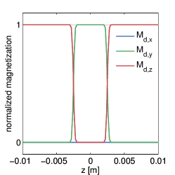
(a) ${M_{d}}$ for single slice (zoom)

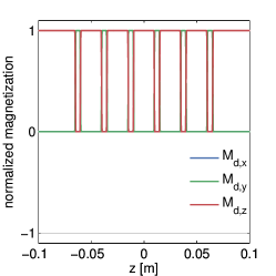
(b) ${M_{d}}$ for SMS 6 (zoom)

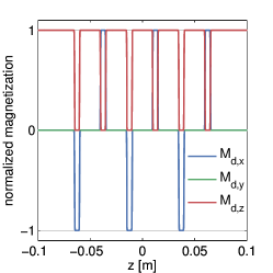
(c) ${M_{d}}$ for phase shifted SMS 6 (zoom)

Figure 1: Desired magnetization for single- (a) and multi-slice (b,c) pulse design

Single-slice excitation

To validate the design procedure, we compute an optimized pulse for a single slice of a given thickness $\Delta_{w}$ and a flip angle of $90\mathrm{°}$, i.e., we set

(14) $${\tilde{M}_{d}}(z)=\begin{cases}\left(0,\sin($$),\cos($$)\right)^{T}&\text{if }|z|<\Delta_{w}/2,\\ (0,0,1)^{T}&\text{else,}\end{cases}$$

as visualized in Fig. 1(a). To reduce Gibbs ringing, this vector is filtered before the optimization with a Gaussian kernel with a full width at half maximum of $1.6\text{\,}\mathrm{mm}$. For comparison, an SLR pulse [38, 31] with an identical temporal resolution and pulse duration is designed to the same specification (slice width, flip angle, full width at half maximum) using the Parks–McClellan (PM) algorithm [38] with a $1\text{\,}\mathrm{\char 37\relax}$ in- and out-of slice ripple as usual [38] and a bandwidth of $2.35\text{\,}\mathrm{kHz}$. To achieve a fully refocused magnetization, the refocusing area of the slice selective gradient for the SLR pulse is increased by $4.1\text{\,}\mathrm{p}\mathrm{e}\mathrm{r}\mathrm{c}\mathrm{e}\mathrm{n}\mathrm{t}$ compared to the OC pulse (Fig. 2(a)).

SMS excitation: phantom

RF pulses for the simultaneous excitation of two, four, and six equidistant rectangular slices with a flip angle of $90\mathrm{°}$ are computed, i.e., we set

(15) $${\tilde{M}_{d}}(z)=\begin{cases}\left(0,\sin($$),\cos($$)\right)^{T}&\text{if $z$ in slice},\\ (0,0,1)^{T}&\text{if $z$ out of slice,}\end{cases}$$

and apply Gauss filtering; see Fig. 1(b) for the case of six slices.

Since PINS pulses are not suitable for axial or axial-oblique slice preference as they generate a periodic slice pattern extending outside the field of interest [49], the optimized pulses are compared with conventional SMS pulses obtained using superposed phase-shifted sinc-based excitation pulses, again for the same slice width, flip angle and full width at half maximum.

SMS excitation: in-vivo

Since multi-slice in-vivo imaging using slice-GRAPPA starts to suffer from g-factor problems for more than three slices, we modify the above-described SMS pulses using a CAIPIRINHA-based excitation pattern [6], which alternates two different pulses to achieve phase-shifted magnetization vectors in order to increase the spatial distance of aliased voxels. Here, the first vector and pulse are identical to those designed for the phantom. For odd slice numbers, the second vector is modified by adding a phase term of $\pi$ to every second slice of the desired magnetization, i.e.,

(16) $${\tilde{M}_{d}}(z)=\begin{cases}\left(0,\pm\sin($$),\cos($$)\right)^{T}&\text{if $z$ in odd/even slice},\\ (0,0,1)^{T}&\text{if $z$ out of slice}\end{cases}$$

(before filtering). For even slice numbers, the transverse pattern has to be further shifted by $\frac{\pi}{2}$, i.e.,

(17) $${\tilde{M}_{d}}(z)=\begin{cases}\left(\pm\sin($$),0,\cos($$)\right)^{T}&\text{if $z$ in even/odd slice},\\ (0,0,1)^{T}&\text{if $z$ out of slice,}\end{cases}$$

see Fig. 1(c) for the case of six slices. The additional phase shift is balanced before reconstruction by subtracting a phase of $\frac{\pi}{2}$ from every second phase-encoding line of the measured k-space data. Since typical relaxation times in the human brain are at least an order of magnitude bigger than the pulse duration, relaxation effects are neglected in the optimization.

The starting point for the optimization is chosen in all cases as ${u}^{0}=[0,\dots,0]$. The control cost parameter is fixed at $\alpha=10^{-4}$ for both the single-slice and the multi-slice optimization. The parameters in Appendix A are set to $\mathrm{tol}_{N}=10^{-9}$, $\mathrm{maxit}_{N}=5$, $\mathrm{tol}_{C}=10^{-6}$, $\mathrm{maxit}_{C}=50$, $\rho_{0}=1$, $\rho_{\max}=2$, $q=2$, $\sigma_{1}=0.03$, $\sigma_{2}=0.25$, $\sigma_{3}=0.7$. All calculations are performed on a workstation with a four-core $64\text{\,}\mathrm{bit}$ processor with $3.1\text{\,}\mathrm{GHz}$ (Intel i$5$-$3350$P) and $16\text{\,}\mathrm{GB}$ of RAM.

3.2 Experimental validation

Fully sampled experimental data for a phantom and a healthy volunteer were acquired on a $3\text{\,}\mathrm{T}$ MR scanner (Magnetom Skyra, Siemens Healthcare, Erlangen, Germany) using the built-in body coil to transmit the RF pulse. The MR signals were received using a body coil for the phantom experiments and a $32$-channel head coil for the in-vivo experiments. A standard Cartesian GRE sequence was modified to import and apply external RF pulses. By changing the read-out gradient from the frequency-axis to the slice direction, the excited slice can be measured and visualized. The single-slice excitation was measured using a water filled sphere with a diameter of $170\text{\,}\mathrm{mm}$. To acquire a high resolution in z-direction, we used a matrix size of $512\text{\times}384$ with a FOV of $250\text{\times}187\text{\,}\mathrm{mm}$ and a bandwidth of $390\text{\,}\mathrm{Hz}$. The echo time was $T_{E}=$ $5\text{\,}\mathrm{ms}$ and the repetition time $T_{R}=$ $2000\text{\,}\mathrm{ms}$ to get fully relaxed magnetization before the next excitation. The SMS phantom experiments were performed using a homogeneous cylinder phantom with diameter of $140\text{\,}\mathrm{mm}$, length of $400\text{\,}\mathrm{mm}$, and relaxation times $T_{1}=$ $102\text{\,}\mathrm{ms}$, $T_{2}=$ $81\text{\,}\mathrm{ms}$, and $T_{2}^{*}=$ $70\text{\,}\mathrm{ms}$. The sequence parameters were $T_{E}=$ $10\text{\,}\mathrm{ms}$, $T_{R}=$ $1000\text{\,}\mathrm{ms}$, bandwidth $390\text{\,}\mathrm{Hz}$, matrix size $512\text{\times}288$, and a field of view of $250\text{\times}141\text{\,}\mathrm{mm}$.

To verify the in-vivo applicability, human brain images of a healthy volunteer were acquired using the above described GRE sequence modified to include the optimized CAIPIRINHA-based pulses. The sequence parameters were set to $T_{E}=$ $10\text{\,}\mathrm{ms}$, $T_{R}=$ $4000\text{\,}\mathrm{ms}$, bandwidth $390\text{\,}\mathrm{Hz}$, matrix size $192\text{\times}120$ and FOV $300\text{\times}187\text{\,}\mathrm{mm}$. After acquisition, the k-space data of the individual slices were separated using an offline slice-GRAPPA ($32$ coils, kernel size of $4\text{\times}4$) reconstruction [42, 9]. The reference scans used in the slice-GRAPPA reconstruction were performed with the same sequence using an optimized single-slice pulse (not shown here). To decrease the scanning time, we acquired $25$ k-space lines ($1\text{/}5$ of the full dataset) around the k-space center for each reference scan. After this separation, a conventional Cartesian reconstruction was performed individually for each slice.

4 Results

Single-slice excitation

Figure 2 shows the results of the design of an RF pulse for the excitation of a single slice of width $\Delta_{w}=$ $5\text{\,}\mathrm{mm}$; see Fig. 1(a). The computed pulse (after $4$ Newton iterations and a total number of $28$ CG steps taking $989\text{\,}\mathrm{s}$ on the above-mentioned workstation is shown in Fig. 2(a). (To indicate the sequence timing, the slice-selective gradient $G_{z}$ – although not part of the optimization – is shown dashed.) It can be seen that $u_{x}(t)$ is similar, but not identical, to a standard sinc shape, and that $u_{y}(t)$ is close to zero, which is expected due to the symmetry of the prescribed slice profile. Figure 2(b) contains a detail of the corresponding transverse magnetization ${M_{xy}}(T)=({M_{x}}(T)^{2}+{M_{y}}(T)^{2})^{1/2}$ obtained from the numerical solution of the Bloch equation, which is confirmed by experimental phantom measurements in Fig. 2(c) and LABEL:sub@fig:single:3. Both simulation and measurement show an excitation with a steep transition between the in- and out-of-slice regions and a homogeneous flip angle distribution across the target slice.

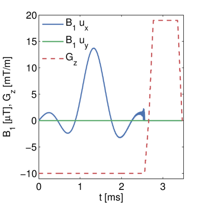
(a) optimized pulse $(u_{x},u_{y})$, gradient $G_{z}$ (fixed)

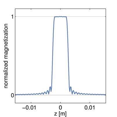
(b) optimized transverse magnetization

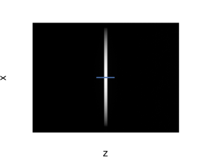
(c) reconstruction of excitation

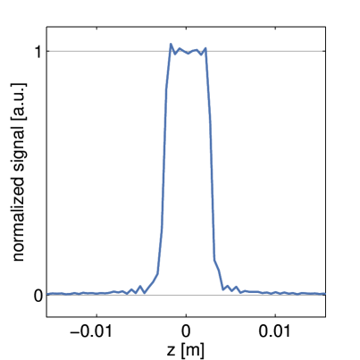
(d) measured transverse magnetization

Figure 2: Optimized pulse and slice profile for single-slice excitation

Figure 3 compares the optimized (OC) pulse with a standard SLR pulse by showing details of the corresponding simulated magnetizations (Fig. 3(a) for OC and Fig. 3(b) for SLR; in both cases the targeted ideal magnetization is shown dashed). It can be seen that the in-slice magnetization of the optimized pulse has oscillations of higher frequency but of much smaller amplitude than that of the SLR pulse. This becomes especially visible when comparing the resulting in-slice phases (Fig. 3(c)).

This is achieved by allowing higher ripples close to the slice while decreasing the amplitude monotonically away from the slice. (Note that only a small central segment of this region is shown in the figures.) This leads to the total root mean squared error (RMSE) and the mean absolute error (MAE) with the ideal rectangular magnetization pattern (Fig. 3(d)) matching the full width at half maximum of both pulses being smaller for the OC pulse ($1.46\text{\times}{10}^{-2}$ and $1.10\text{\times}{10}^{-4}$, respectively) compared to the SLR pulse ($1.62\text{\times}{10}^{-2}$ and $2.27\text{\times}{10}^{-4}$, with an equal power demand for both pulses.

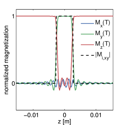
(a) simulated magnetization (OC)

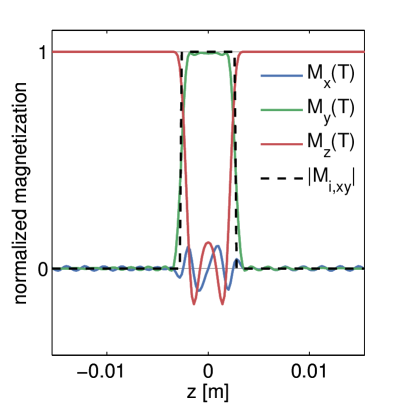
(b) simulated magnetization (SLR)

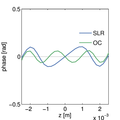
(c) in-slice phase

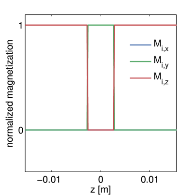
(d) ideal magnetization

Figure 3: Comparison of SLR and OC pulse

SMS excitation: phantom

Figure 4 shows the results of the design of RF pulses for simultaneous excitation of two, four and six equidistant slices with a separation of $25\text{\,}\mathrm{mm}$ and a thickness $\Delta_{w}=$ $5\text{\,}\mathrm{mm}$; see Fig. 1(b). The computational effort in all cases is similar to that in the single-slice case. The corresponding computed pulses are shown in Figs. 4(a) to LABEL:sub@fig:sms:a6. A graphical analysis shows that instead of higher amplitudes, the optimization distributes the total RF power (which increases with the number of slices) more uniformly over the pulse length. A central section of the corresponding optimized slice profiles are given in Figs. 4(d) to LABEL:sub@fig:sms:b6. It can be seen that all slices have a sharp profile which does not deteriorate as the number of slices increases (although it decreases slightly farther from the center and the bandwidth is slightly reduced). These results are validated by the experimental phantom measurements using the computed pulses: Figs. 4(g) to LABEL:sub@fig:sms:c6 show the reconstructed excitation inside the phantom, while Figs. 4(j) to LABEL:sub@fig:sms:d6 show the measured slice profiles along a cut parallel to the $x$-axis in the center of the previous images.

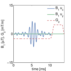
(a) optimized pulse (2 slices)

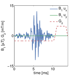
(b) optimized pulse (4 slices)

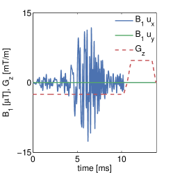
(c) optimized pulse (6 slices)

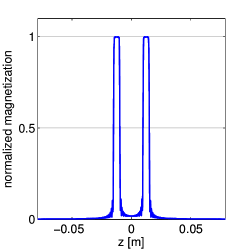
(d) optimized slice profile (2)

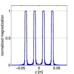
(e) optimized slice profile (4)

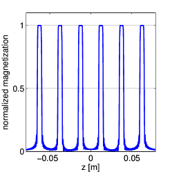
(f) optimized slice profile (6)

(g) reconstructed excitation (2)

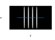
(h) reconstructed excitation (4)

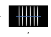
(i) reconstructed excitation (6)

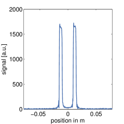
(j) measured slice profile (2)

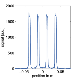
(k) measured slice profile (4)

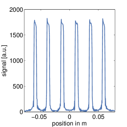
(l) measured slice profile (6)

Figure 4: Optimized pulses and slice profiles for SMS excitation (phantom)

A quantitative comparison of SLR and OC-based SMS pulses from one to six simultaneous slices is given in Table 1, which shows both the power requirement of the computed pulses, both in total B₁ energy

(18) $$\|{B_{1,x}}\|_{2}^{2}=\int_{0}^{T}|B_{1}u_{x}(t)|^{2}\,dt$$

and in peak B₁ amplitude

(19) $$\|{B_{1,x}}\|_{\infty}=\max_{t\in[0,T]}|B_{1}u_{x}(t)|,$$

as well as the mean absolute error (MAE) with respect to the ideal (unfiltered) slice profiles for the in-slice and the out-of-slice regions. While both methods lead to a linear increase of the total energy with the number of slices, the peak amplitude increases more slowly for the OC pulses than for the conventional pulses. Furthermore, we remark that the peak B₁ amplitude for four, five and six slices remain similar. Regarding the corresponding slice profiles, the OC pulses lead to a significantly lower MAE in both the in-slice and out-of-slice regions compared to the SLR pulses. Visual inspection of Figs. 4(d) to LABEL:sub@fig:sms:b6 shows that this is due to the fact that the out-of-slice ripples are concentrated around the in-slice regions while quickly decaying away from them.

Table 1: Comparison of B₁ power and the mean absolute error (MAE) of the transverse magnetization after excitation for conventional and OC based SMS pulses

	$\|B_{1,x}\|_{2}^{2}$		$\|B_{1,x}\|_{\infty}$		MAE in-slice		MAE out-of-slice
	[a.u.]		[$\mathrm{\SIUnitSymbolMicro T}$]		[a.u.]		[a.u.]
slices	conv	OC	conv	OC	conv	OC	conv	OC
$1$	$19.5$	$19.5$	$3.5$	$3.49$	$0.062$	$0.052$	$0.0039$	$0.0014$
$2$	$38.9$	$38.1$	$7.0$	$6.78$	$0.060$	$0.052$	$0.0040$	$0.0018$
$3$	$58.4$	$57.2$	$10.5$	$10.02$	$0.054$	$0.053$	$0.0039$	$0.0030$
$4$	$77.9$	$76.3$	$14.0$	$12.13$	$0.065$	$0.045$	$0.0086$	$0.0031$
$5$	$97.3$	$95.5$	$17.5$	$11.38$	$0.059$	$0.053$	$0.0078$	$0.0051$
$6$	$116.8$	$113.9$	$21.0$	$12.63$	$0.068$	$0.053$	$0.0075$	$0.0067$

Finally, we illustrate the influence of the regularization parameter $\alpha$ in Table 2, where the root of mean square error (RMSE), the total B₁ energy as well as the B₁ peak of the OC SMS 6 pulses is shown for different values of the control cost parameter $\alpha$. As can be seen, a bigger $\alpha$ leads to an increase in the error between desired and controlled magnetization while both the total B₁ power and the peak B₁ amplitude are reduced, although these effects amount to less than $20\text{\,}\mathrm{p}\mathrm{e}\mathrm{r}\mathrm{c}\mathrm{e}\mathrm{n}\mathrm{t}$ over a range of parameters spanning two orders of magnitude. This demonstrates that the results presented here are robust with respect to the choice of the control cost parameter.

Table 2: Comparison of RMSE, B₁ power and B₁ peak for different values of $\alpha$

$\alpha$	RMSE	$\|B_{1,x}\|_{2}^{2}$	$\|B_{1,x}\|_{\infty}$
[a.u.]	[a.u.]	[a.u.]	[$\mathrm{\SIUnitSymbolMicro T}$]
$1\text{\times}{10}^{-5}$	$2.374\text{\times}{10}^{-2}$	$117.0$	$12.75$
$5\text{\times}{10}^{-5}$	$2.375\text{\times}{10}^{-2}$	$115.1$	$12.71$
$1\text{\times}{10}^{-4}$	$2.377\text{\times}{10}^{-2}$	$113.9$	$12.62$
$5\text{\times}{10}^{-4}$	$2.437\text{\times}{10}^{-2}$	$106.7$	$12.14$
$1\text{\times}{10}^{-3}$	$2.591\text{\times}{10}^{-2}$	$98.9$	$11.63$

SMS excitation: in-vivo

The CAIPIRINHA-based modifications to the SMS pulse design (see Fig. 1(c)) are illustrated in Fig. 5 (showing the case of five slices for the sake of variation). Figure 5(a) shows the unmodified pulse, which differs in structure from the cases with an even number of slices in, e.g., Fig. 4(c) due to the different symmetry of the slice profile (see Fig. 5(b)). On the other hand, the pulse is very similar to the modified pulse for the alternating phase shift; see Fig. 5(c) for the computed pulse and Fig. 5(d) for the resulting slice profile. For illustration, a slice-aliased reconstruction of the acquired in-vivo data using this pulse sequence is shown in Fig. 5(e).

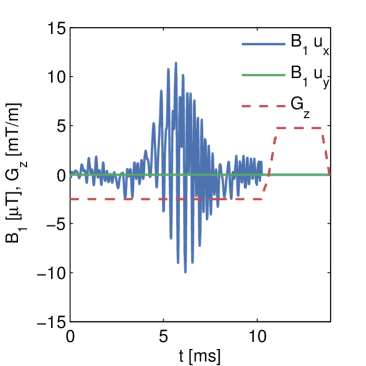
(a) optimized pulse (no shift)

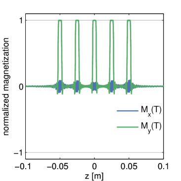
(b) optimized slice profile of (a)

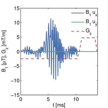
(c) optimized pulse (phase shift)

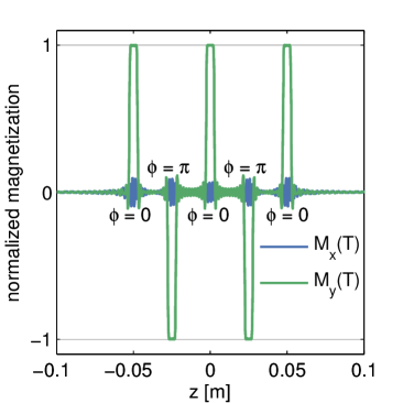
(d) optimized slice profile of (c)

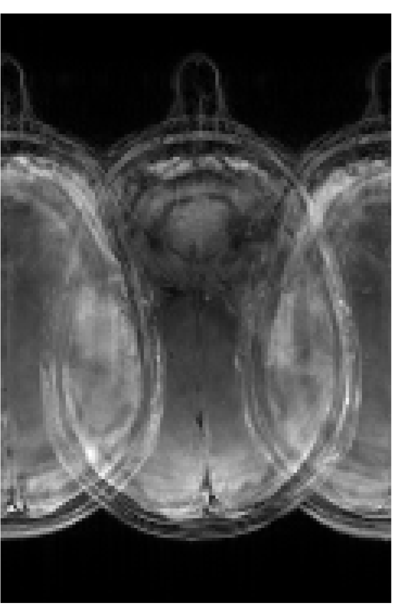
(e) slice-aliased reconstruction

Figure 5: Optimized pulses, slice profiles and slice-aliased Cartesian reconstruction for CAIPIRINHA-based SMS excitation pattern (five slices)

z readout

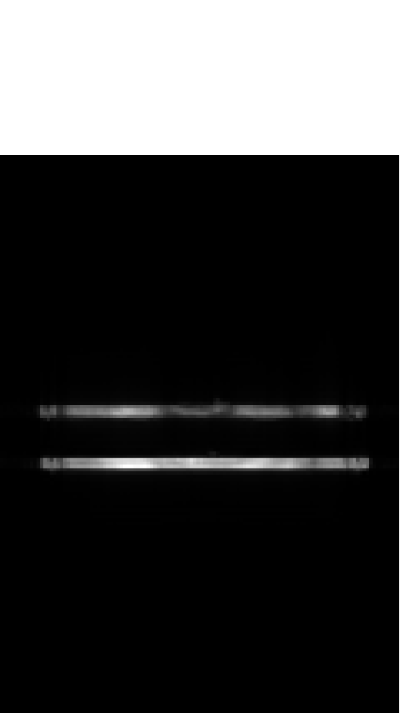
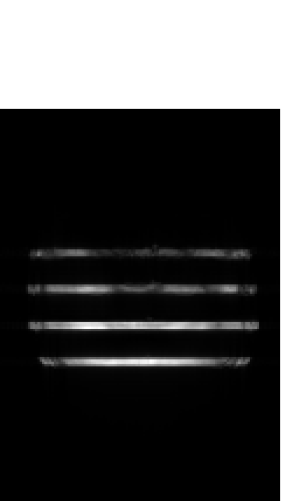
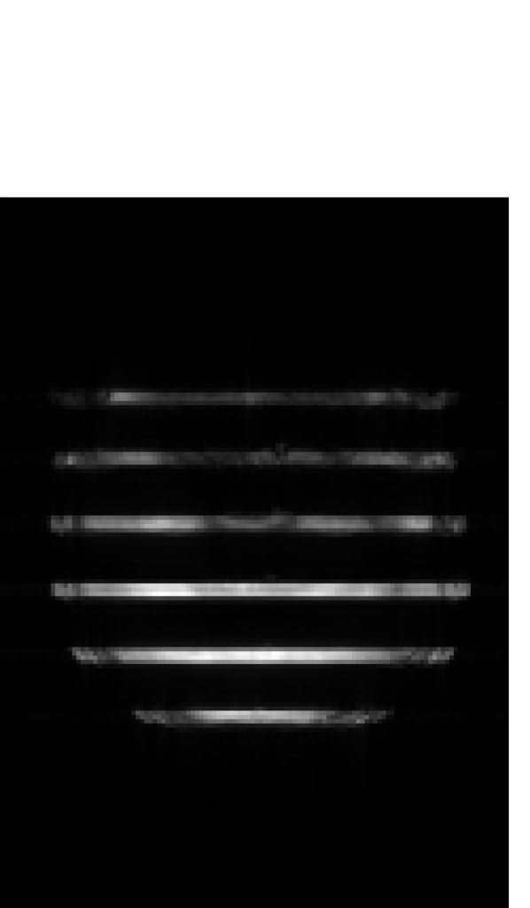
sG reconstruction

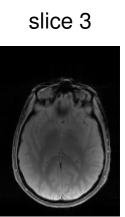
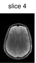
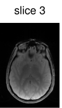
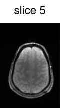
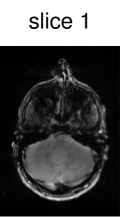
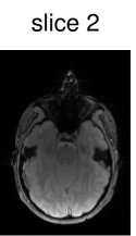
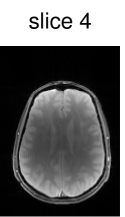
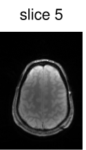
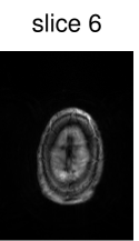
Figure 6: Slice-GRAPPA reconstruction of in-vivo data using CAIPIRINHA-based SMS excitation pattern for two (top), four (middle) and six (bottom) slices (left: conventional reconstruction showing the collapsed data in slice-encoding direction; right: reconstruction of GRAPPA-separated slices)

Figure 6 shows the image reconstruction using optimized RF pulses for simultaneous excitation of two, four and six slices with the same slice separation and thickness as above. As can be seen clearly in the first column, all three pulses lead to the desired excitation pattern in-vivo as well. The remaining columns show the slice-GRAPPA reconstructions, which illustrate that the excitation is uniform across the field of view.

5 Discussion

Our optimization approach is related to the basic ideas presented by Conolly et al. [12]. In the context of MRI, the implementation of this principle was also carried out by other groups using gradient [56, 20] and quasi-Newton [51] methods. However, these methods do not make full use of second-order information and therefore achieve at best superlinear convergence. In contrast, our Newton method makes use of exact second derivatives and is therefore quadratically convergent. In particular, the main contribution of our work is the efficient computation of exact Hessian actions using the adjoint approach and its implementation in a matrix-free trust-region CG–Newton method. The use of exact derivatives speeds up convergence of the CG method, while the trust-region framework guarantees global convergence and terminates the CG method early especially at the beginning of the optimization. Both techniques save CG steps and therefore computations of Hessian actions, allowing the use of second-order information with limited computational effort and memory requirements. Since computing a Hessian action incurs the same computational cost as a gradient evaluation (i.e., the solution of two ODEs; compare (6) with (10)), we were able to compute a minimizer, e.g., for the single-slice example, with a computational effort corresponding to $32$ gradient evaluations ($4$ for the right-hand side in each Newton iteration and $28$ for the Hessian action in each CG iteration). This is less than the same number of iterations of a gradient or quasi-Newton method with line search (required in this case for global convergence), demonstrating the efficiency of the proposed approach. Therefore, our method can be used to compute RF pulses with a high temporal resolution, allowing the design of pulses for a desired magnetization on a very fine spatial scale, in particular for the excitation of a sharp slice profile.

Furthermore, the proposed algorithm does not require an educated initial guess for global convergence (to a local minimizer, which might depend on the initial guess if more than one exists) and allows for pulse optimization in non-standard situations where no analytic RF pulse exists (e.g., for large flip angles). Compared to design methods using a simplification or approximation of the Bloch equation [37, 38], our OC based approach is capable of including relaxation terms. However, for standard in-vivo imaging applications of the human head, the relevant relaxation times are very long compared to the RF pulse duration. Thus, in our examples the influence of relaxation during excitation on the designed pulses is insignificant and has been neglected in the optimization process (although the inclusion may be indicated for other applications). The presented direct design approach allows to specify the desired magnetization in x-, y- and z-direction independently for every point in the field of view. This spatial independence of each control point allows to directly apply parallel computing to speed up the optimization process. While real-time optimization was not the aim of this work, a proof-of-concept implementation of the proposed approach on a GPU system (CUDA, double precision, GeForce GTX $550$ Ti with $192$ cores and $1024\text{\,}\mathrm{MB}$ of RAM) shows an average speedup of $135$ (e.g., $6.8\text{\,}\mathrm{s}$ instead of $989\text{\,}\mathrm{s}$ for the single-slice example) while yielding identical results, thus making patient-specific design feasible as well as making the gap between OC and SLR pulse design nearly negligible. This allows efficient and fast generation of accurate slice profiles – important for minimal slice gaps, optimal contrast and low systematic errors in quantitative imaging – for arbitrary flip angles and even for specialized pulses such as refocusing or inversion.

In particular, our approach can be used to design pulses for the simultaneous excitation of multiple slices, which increases the temporal efficiency of advanced imaging techniques such as diffusion tensor imaging, functional imaging or dynamic scans. In these contexts, SMS excitation is successfully used to reduce the total imaging time [30, 36, 17, 49]; however, the peak B₁ amplitude of conventional SMS pulses is one of the main restrictions of applying SMS imaging to high-field systems [49]. The performed studies show that compared to conventional SMS design, the presented procedure yields pulses with a reduced B₁ peak amplitude (e.g., $40\text{\,}\mathrm{\char 37\relax}$ reduction for six simultaneous slices). Depending on the desired temporal resolution, the bandwidth and the slice profiles of the outer slices are slightly changed, which results in a decreased B₁ peak amplitude. It could be shown that the peak B₁ amplitude does not increase linearly with the number of slices, while the power requirement per slice remains constant and the overall power consumption is comparable to that of conventional pulses. To further reduce the SAR it is necessary to either change the excitation velocity using a time-varying slice selective gradient [13], or to extend the pulse design to parallel transmit [25, 55, 39, 22]. Furthermore, our OC-based pulses produce sharp slice profiles with a lower mean absolute error compared to the used PM-based SLR pulse, both in- and out-of-slice, at the cost of slightly larger out-of-slice ripples close to the in-slice regions. Of course, the ripple behavior of the SLR pulse can be balanced with the transition steepness by using different digital filter design methods (i.e. PM for minimizing the maximum ripple or a least squares linear-phase FIR filter for minimizing integrated squared error). The OC ripple amplitude close to the transition band can be further controlled by using offset-dependent weights as demonstrated by Skinner et al. [47]. In addition, the computational complexity of OC methods is significantly higher than for direct or linearized methods. This implies that OC-based pulse design is advantageous in situations where high in-slice contrast and low B₁ peak amplitude are important, while SLR pulses should be used when minimal near-slice excitation and computational effort are crucial.

The presented OC approach is able to avoid some possible disadvantages of previously proposed design methods for SMS excitation. In particular, the OC design method prescribes each slice with the same uniform echo-time and phase in comparison to time-shifted [2], phase relaxation [53] and nonlinear phase design techniques [57, 44]. On the other hand, some of their features such as different echo times [2] or a non-uniform phase pattern [53, 57, 44] (e.g., for spin echo experiments) can be incorporated in our approach to further reduce the B₁ peak amplitude. It also should be possible to combine the OC design method with other techniques analogous to MultiPINS [16, 18] that combine PINS with conventional multiband pulses for a further reduction of SAR. Finally, the phantom and in-vivo experiments demonstrate that it is possible to simply replace standard pulses by optimized pulses in existing imaging sequences, and that the proposed method is therefore well suited for application in a wide range of imaging situations in MRI.

6 Conclusions

This paper demonstrates a novel general-purpose implementation of RF pulse optimization based on the full time-dependent Bloch equation and a highly efficient second-order optimization technique assuring global convergence to a local minimizer, which allows large-scale optimization with flexible problem-specific constraints. The power and applicability of this technique was demonstrated for SMS, where a reduced B₁ peak amplitude allows exciting a higher number of simultaneous slices or achieving a higher flip angle. Phantom and in-vivo measurements (on a $3\text{\,}\mathrm{T}$ scanner) verified these findings for optimized single- and multi-slice pulses. Even for a large number of simultaneously acquired slices, the reconstructed images show good image quality and thus the applicability of the optimized RF pulses for practical imaging applications. While the computational requirements for optimal control approaches are of course significantly greater than for, e.g., SLR-based approaches, a proof-of-concept GPU implementation indicates that this gap can be sufficiently narrowed to make patient-specific design feasible.

Due to the flexibility of the optimal control formulation and the efficiency of our optimization strategy, it is possible to consider field inhomogeneities (B₁, B₀), design complex RF pulses for parallel transmit, or to extend the framework to include pointwise constraints due to hardware limits such as peak B1 amplitude and slew rate.

Appendix A Trust-region algorithm

[H] Trust-region CG-Newton algorithm Trust region parameters $\mathrm{tol}_{N}$, $\mathrm{maxit}_{N}$, $\mathrm{tol}_{C}$, $\mathrm{maxit}_{C}$, $\rho_{0}$, $\rho_{\max}$, $q>1$, $0<\sigma_{1}<\sigma_{2}<\sigma_{3}<1$ Control ${u}$

Set ${u}^{0}\equiv 0,\quad k=0,\quad{g}\equiv 1,\quad\rho=\rho_{0}$*initialization (*[f]TR-Newton step)$\|g\|>\mathrm{tol}_{N}$ and $k<\mathrm{maxit}_{N}$ Compute gradient ${g}({u}^{k})$  Set ${p}^{0}={r}^{0}=-{g}({u}^{k})$, $\delta{u}=0$, $i=0$  (*[f]TR-CG step)$\|{r}^{i}\|>\mathrm{tol}_{C}\|{r}^{0}\|$ and $i<\mathrm{maxit}_{C}$ Compute ${H}({u}^{k}){p}^{i}$  (*[f]negative curvature: CG fails)$\langle{p}^{i},{H}({u}^{k}){p}^{i}\rangle<\varepsilon$ Compute $\max\{\tau:\|\delta{u}+\tau{p}^{i}\|\leq\rho\}$*go to boundary of trust region Set $\delta{u}=\delta{u}+\tau{p}^{i}$; break

Compute $\alpha=\|{r}^{i}\|/\langle{p}^{i},{H}({u}^{k}){p}^{i}\rangle$  (*[f]step too large: model not trusted)$\|\delta{u}+\alpha{p}^{i}\|\geq\rho$ Compute $\max\{\tau:\|\delta{u}+\tau{p}^{i}\|\leq\rho\}$*go to boundary of trust region Set $\delta{u}=\delta{u}+\tau{p}^{i}$; break  Set ${r}^{i+1}={r}^{i}-\alpha{H}({u}^{k}){p}^{i}$  Set ${p}^{i+1}={r}^{i+1}+\|{r}^{i+1}\|^{2}/\|{r}^{i}\|^{2}{p}^{i}$  Set $\delta{u}=\delta{u}+\alpha{p}^{i}$, $i=i+1$  Compute $\delta J_{a}=J({u}^{k})-J({u}^{k}+\delta{u})$*actual function decrease Compute $\delta J_{m}=-\tfrac{1}{2}\langle\delta{u},{H}({u}^{k})\delta{u}\rangle-\langle\delta{u},{g}({u}^{k})\rangle$*predicted function decrease (*[f]sufficient decrease)$\delta J_{a}>\varepsilon$ and $\delta J_{a}>\sigma_{1}\delta J_{m}$ Set ${u}^{k+1}={u}^{k}+\delta{u}$*accept step (*[f]step accepted, model good)$\delta J_{a}>\varepsilon$ and $|\delta J_{a}/\delta J_{m}-1|\leq 1-\sigma_{3}$ Set $\rho=\min\left\{q\rho,\rho_{\max}\right\}$*increase radius (*[f]step rejected, no decrease)$\delta J_{a}\leq\varepsilon$ Set $\rho=\rho/q$*decrease radius (*[f]model bad)$\delta J_{a}<\sigma_{2}\delta J_{m}$ Set $\rho=\rho/q$*decrease radius

Appendix B Discretization

Cost functional:

$$J({M},{u})=\frac{1}{2}\sum_{i=1}^{Z}\Delta z_{i}|{M}_{N,i}-{M_{d}}(z_{i})|_{2}^{2}+\frac{\alpha}{2}\sum_{m=1}^{N}\Delta t_{m}|{u}_{m}|_{2}^{2}$$

Bloch equation

for all $i=1,\dots,Z$:

$$\left[{I}-\frac{\Delta t_{m}}{2}{A}({u}_{m};z_{i})\right]{M}_{m,i} =\left[{I}+\frac{\Delta t_{m}}{2}{A}({u}_{m};z_{i})\right]{M}_{m-1,i}+\Delta t_{m}{b},\quad m=1,\dots,N$$

$${M}_{0,i} ={M^{0}}(z_{i})$$

Adjoint equation

for all $i=1,\dots,Z$:

$$\left[{I}-\frac{\Delta t_{m}}{2}{A}({u}_{m};z_{i})^{T}\right]{P}_{m,i} =\left[{I}+\frac{\Delta t_{m+1}}{2}{A}({u}_{m+1};z_{i})^{T}\right]{P}_{m+1,i},\quad m=1,\dots,N-1$$

$$\left[{I}-\frac{\Delta t_{N}}{2}{A}({u}_{N};z_{i})^{T}\right]{P}_{N,i} ={M}_{N,i}-{M_{d}}(z_{i})$$

Discrete gradient

for all $m=1,\dots,N_{u}$:  $\bar{{M}}_{m}:=\frac{1}{2}({M}_{m}+{M}_{m-1})$,

$${g}_{m}=\alpha{u}_{m}+\gamma B_{1}\begin{pmatrix}\sum_{i=1}^{Z}\Delta z_{i}\left({P}_{m,i}^{T}{A_{1}}\bar{{M}}_{m,i}\right)\\ \sum_{i=1}^{Z}\Delta z_{i}\left({P}_{m,i}^{T}{A_{2}}\bar{{M}}_{m,i}\right)\end{pmatrix}$$

Linearized state equation

for all $i=1,\dots,Z$:

$$\left[{I}-\frac{\Delta t_{m}}{2}{A}(u_{m};z_{i})\right]\delta{M}_{m,i} =\left[{I}+\frac{\Delta t_{m}}{2}{A}(u_{m};z_{i})\right]\delta{M}_{m-1,i}+\Delta t_{m}{A^{\prime}}(\delta u_{m})\bar{{M}}_{m,i},\quad m=1,\dots,N$$

$$\delta{M}_{0,i} =0$$

Linearized adjoint equation

for all $i=1,\dots,Z$:

$$\left[{I}-\frac{\Delta t_{m}}{2}{A}(u_{m};z_{i})^{T}\right]\delta{P}_{m,i} =\left[{I}+\frac{\Delta t_{m+1}}{2}{A}(u_{m+1};z_{i})^{T}\right]\delta{P}_{m+1,i}+\frac{\Delta t_{m}}{2}{A^{\prime}}(\delta{u}_{m})^{T}P_{m,i}$$

$$+\frac{\Delta t_{m+1}}{2}{A^{\prime}}(\delta{u}_{m+1})^{T}{P}_{m+1,i},\quad m=1,\dots,N-1$$

$$\left[{I}-\frac{\Delta t_{N}}{2}{A}(u_{N};z_{i})^{T}\right]\delta{P}_{N,i} =\delta{M}_{N,i}+\frac{\Delta t_{N}}{2}{A^{\prime}}(\delta{u}_{N})^{T}{P}_{N,i}$$

Discrete Hessian action

for all $m=1,\dots,N_{u}$:  $\bar{\delta{M}_{m}}:=\frac{1}{2}(\delta{M}_{m}+\delta{M}_{m-1})$

$$\quad[{H}({u}){h}]_{m}=\alpha{h}_{m}+\gamma B_{1}\begin{pmatrix}\sum_{i=1}^{Z}\Delta z_{i}\left(\delta{P}_{m,i}^{T}{A_{1}}{\bar{M}}_{m,i}+{P}_{m,i}^{T}{A_{1}}{\bar{\delta M}}_{m,i}\right)\\ \sum_{i=1}^{Z}\Delta z_{i}\left(\delta{P}_{m,i}^{T}{A_{2}}{\bar{M}}_{m,i}+{P}_{m,i}^{T}{A_{2}}{\bar{\delta M}}_{m,i}\right)\end{pmatrix}$$

References

- [1] Christopher K. Anand, Alex D. Bain, Andrew T. Curtis and Zhenghua Nie “Designing optimal universal pulses using second-order, large-scale, non-linear optimization” In Journal of Magnetic Resonance 219, 2012, pp. 61–74 DOI: doi:10.1016/j.jmr.2012.04.004
- [2] Edward J. Auerbach et al. “Multiband accelerated spin-echo echo planar imaging with reduced peak RF power using time-shifted RF pulses” In Magnetic Resonance in Medicine 69.5, 2013, pp. 1261–1267 DOI: 10.1002/mrm.24719
- [3] Priti Balchandani, John Pauly and Daniel Spielman “Designing adiabatic radio frequency pulses using the Shinnar–Le Roux algorithm” In Magnetic Resonance in Medicine 64.3, 2010, pp. 843–851 DOI: 10.1002/mrm.22473
- [4] Roland Becker, Dominik Meidner and Boris Vexler “Efficient numerical solution of parabolic optimization problems by finite element methods” In Optimization Methods and Software 22.5, 2007, pp. 813–833 DOI: 10.1080/10556780701228532
- [5] Bernard Bonnard, Mathieu Claeys, Olivier Cots and Pierre Martinon “Geometric and numerical methods in the contrast imaging problem in nuclear magnetic resonance” In Acta Applicandae Mathematicae online first, 2014 DOI: 10.1007/s10440-014-9947-3
- [6] F.. Breuer et al. “Controlled aliasing in volumetric parallel imaging (2D CAIPIRINHA)” In Magnetic Resonance in Medicine 55.3, 2006, pp. 549–556 DOI: 10.1002/mrm.20787
- [7] M.. Buonocore “RF pulse design using the inverse scattering transform” In Magnetic Resonance in Medicine 29.4, 1993, pp. 470–477 DOI: 10.1002/mrm.1910290408
- [8] Graeme M. Bydder, Gary D. Fullerton and Ian R. Young “MRI of tissues with short T2s or T2*s” Wiley, 2012
- [9] Stephen F. Cauley et al. “Interslice leakage artifact reduction technique for simultaneous multislice acquisitions” In Magnetic Resonance in Medicine 72.1, 2014, pp. 93–102 DOI: 10.1002/mrm.24898
- [10] Gabriele Ciaramella and Alfio Borzi “SKRYN: A fast semismooth-Krylov–Newton method for controlling Ising spin systems” In Computer Physics Communications 190, 2015, pp. 213–223 DOI: 10.1016/j.cpc.2015.01.006
- [11] Gabriele Ciaramella, Alfio Borzi, G. Dirr and D. Wachsmuth “Newton methods for the optimal control of closed quantum spin systems” In SIAM Journal on Scientific Computing 37, 2015, pp. A319–A346 DOI: 10.1137/140966988
- [12] Steven Conolly, Dwight Nishimura and Albert Macovski “Optimal control solutions to the magnetic resonance selective excitation problem” In Medical Imaging, IEEE Transactions on MI-5.2, 1986, pp. 106–115 DOI: 10.1109/TMI.1986.4307754
- [13] Steven Conolly, Dwight Nishimura, Albert Macovski and Gary Glover “Variable-rate selective excitation” In Journal of Magnetic Resonance 78, 1988, pp. 440–458 DOI: 10.1016/0022-2364(88)90131-X
- [14] P. Fouquieres, S.G. Schirmer, S.J. Glaser and Ilya Kuprov “Second order gradient ascent pulse engineering” In Journal of Magnetic Resonance 212.2, 2011, pp. 412–417 DOI: 10.1016/j.jmr.2011.07.023
- [15] Ludovic Rochefort, Xavier Maître, Jacques Bittoun and Emmanuel Durand “Velocity-selective RF pulses in MRI” In Magnetic Resonance in Medicine 55.1, 2006, pp. 171–176 DOI: 10.1002/mrm.20751
- [16] Cornelius Eichner, Lawrence L. Wald and Kawin Setsompop “A low power radiofrequency pulse for simultaneous multislice excitation and refocusing” In Magnetic Resonance in Medicine 72.4, 2014, pp. 949–953 DOI: 10.1002/mrm.25389
- [17] D.. Feinberg and K. Setsompop “Ultra-fast MRI of the human brain with simultaneous multi-slice imaging” In Journal of Magnetic Resonance 229, 2013, pp. 90–100 DOI: 10.1016/j.jmr.2013.02.002
- [18] Borjan A. Gagoski et al. “RARE/turbo spin echo imaging with simultaneous multislice Wave-CAIPI” In Magnetic Resonance in Medicine 73.3, 2015, pp. 929–938 DOI: 10.1002/mrm.25615
- [19] J.. Gezelter and R. Freeman “Use of neural networks to design shaped radiofrequency pulses” In Journal of Magnetic Resonance (1969) 90.2, 1990, pp. 397–404 DOI: 10.1016/0022-2364(90)90149-4
- [20] W. Grissom et al. “Fast large-tip-angle multidimensional and parallel RF pulse design in MRI” In Medical Imaging, IEEE Transactions on 28.10, 2009, pp. 1548–1559 DOI: 10.1109/TMI.2009.2020064
- [21] William A. Grissom, Graeme C. McKinnon and Mika W. Vogel “Nonuniform and multidimensional Shinnar–Le Roux RF pulse design method” In Magnetic Resonance in Medicine 68.3, 2012, pp. 690–702 DOI: 10.1002/mrm.23269
- [22] Bastien Guérin et al. “Design of parallel transmission pulses for simultaneous multislice with explicit control for peak power and local specific absorption rate” In Magnetic Resonance in Medicine 73.5, 2014, pp. 1946–1953 DOI: 10.1002/mrm.25325
- [23] M. Hinze, R. Pinnau, M. Ulbrich and S. Ulbrich “Optimization with PDE Constraints” 23, Mathematical Modelling: Theory and Applications Springer, New York, 2009 DOI: 10.1007/978-1-4020-8839-1
- [24] Michael Hinze and Karl Kunisch “Second order methods for optimal control of time-dependent fluid flow” In SIAM Journal on Control and Optimization 40.3, 2001, pp. 925–946 DOI: 10.1137/S0363012999361810
- [25] Ulrich Katscher et al. “3D RF shimming using multi-frequency excitation” In Proc. ISMRM 16, 208, pp. 1311
- [26] A.. Khalifa, Abou-Bakr M. Youssef and Y.. Kadah “Optimal design of RF pulses with arbitrary profiles in magnetic resonance imaging” In Engineering in Medicine and Biology Society, 2001. Proceedings of the 23rd Annual International Conference of the IEEE 3, 2001, pp. 2296–2299 DOI: 10.1109/IEMBS.2001.1017234
- [27] Navin Khaneja et al. “Optimal control of coupled spin dynamics: design of NMR pulse sequences by gradient ascent algorithms” In Journal of Magnetic Resonance 172.2, 2005, pp. 296–305 DOI: 10.1016/j.jmr.2004.11.004
- [28] D.. Knoll and D.. Keyes “Jacobian-free Newton–Krylov methods: a survey of approaches and applications” In Journal of Computational Physics 193.2, 2004, pp. 357–397 DOI: 10.1016/j.jcp.2003.08.010
- [29] M. Lapert et al. “Exploring the physical limits of saturation contrast in magnetic resonance imaging” In Scientific Reports 2, 2012 DOI: 10.1038/srep00589
- [30] D.. Larkman et al. “Use of multicoil arrays for separation of signal from multiple slices simultaneously excited” In Journal of Magnetic Resonance Imaging 13.2, 2001, pp. 313–317 DOI: 10.1002/1522-2586(200102)13:2<313::AID-JMRI1045>3.0.CO;2-W
- [31] K.. Lee “General parameter relations for the Shinnar–Le Roux pulse design algorithm” In Journal of Magnetic Resonance 186.2, 2007, pp. 252–258 DOI: 10.1016/j.jmr.2007.03.010
- [32] Chao Ma and Zhi-Pei Liang “Design of multidimensional Shinnar–Le Roux radiofrequency pulses” In Magnetic Resonance in Medicine 73.2, 2015, pp. 633–645 DOI: 10.1002/mrm.25179
- [33] S. Müller “Multifrequency selective RF pulses for multislice MR imaging” In Magnetic Resonance in Medicine 6.3, 1988, pp. 364–371 DOI: 10.1002/mrm.1910060315
- [34] Dwight G. Nishimura “Principles of Magnetic Resonance Imaging” Standford University, 1996
- [35] D.. Norris, P.. Koopmans, R. Boyacioğlu and M. Barth “Power independent of number of slices (PINS) radiofrequency pulses for low-power simultaneous multislice excitation” In Magnetic Resonance in Medicine 66.5, 2011, pp. 1234–1240 DOI: 10.1002/mrm.23152
- [36] R.G. Nunes, J.. Hajnal, X. Golay and D.. Larkman “Simultaneous slice excitation and reconstruction for single shot EPI” In Proc. ISMRM 14, 2006, pp. 293
- [37] J. Pauly, D. Nishimura and A. Macovski “A k-space analysis of small-tip-angle excitation” In Journal of Magnetic Resonance (1969) 213.2, 1989, pp. 544–557 DOI: 10.1016/0022-2364(89)90265-5
- [38] John Pauly, Patrick Le Roux, Dwight Nishimura and Albert Macovski “Parameter relations for the Shinnar–Le Roux selective excitation pulse design algorithm” In Medical Imaging, IEEE Transactions on 10.1, 1991, pp. 53–65 DOI: 10.1109/42.75611
- [39] Benedikt A. Poser et al. “Simultaneous multislice excitation by parallel transmission” In Magnetic Resonance in Medicine 71.4, 2014, pp. 1416–1427 DOI: 10.1002/mrm.24791
- [40] Fadil Santosa and William W. Symes “Computation of the Hessian for least-squares solutions of inverse problems of reflection seismology” In Inverse Problems 4.1, 1988, pp. 211 DOI: 10.1088/0266-5611/4/1/017
- [41] K. Setsompop et al. “Improving diffusion MRI using simultaneous multi-slice echo planar imaging” In NeuroImage 63.1, 2012, pp. 569–580 DOI: 10.1016/j.neuroimage.2012.06.033
- [42] Kawin Setsompop et al. “Blipped-controlled aliasing in parallel imaging for simultaneous multislice echo planar imaging with reduced g-factor penalty” In Magnetic Resonance in Medicine 67.5, 2012, pp. 1210–1224 DOI: 10.1002/mrm.23097
- [43] A. Sharma et al. “kT-PINS RF pulses for low-power field inhomogeneity-compensated multislice excitation” In Proc. ISMRM 21, 2013, pp. 44
- [44] Anuj Sharma, Michael Lustig and William A. Grissom “Root-flipped multiband refocusing pulses” In Magnetic Resonance in Medicine Early View, 2015 DOI: 10.1002/mrm.25629
- [45] Jun Shen “Delayed-focus pulses optimized using simulated annealing” In Journal of Magnetic Resonance 149.2, 2001, pp. 234–238 DOI: 10.1006/jmre.2001.2306
- [46] Thomas E. Skinner et al. “New strategies for designing robust universal rotation pulses: Application to broadband refocusing at low power” In Journal of Magnetic Resonance 216, 2012, pp. 78–87 DOI: 10.1016/j.jmr.2012.01.005
- [47] Thomas E. Skinner, Naum I. Gershenzona, Manoj Nimbalkar and Steffen J. Glaser “Optimal control design of band-selective excitation pulses that accommodate relaxation and RF inhomogeneity” In Journal of Magnetic Resonance 217, 2012, pp. 53–60 DOI: 10.1016/j.jmr.2012.02.007
- [48] Trond Steihaug “The conjugate gradient method and trust regions in large scale optimization” In SIAM Journal on Numerical Analysis 20.3, 1983, pp. 626–637 DOI: 10.1137/0720042
- [49] K. Uğurbil et al. “Pushing spatial and temporal resolution for functional and diffusion MRI in the Human Connectome Project” In NeuroImage 80, 2013, pp. 80–104 DOI: 10.1016/j.neuroimage.2013.05.012
- [50] J.. Ulloa, M. Guarini, A. Guesalaga and P. Irarrazaval “Chebyshev series for designing RF pulses employing an optimal control approach” In Medical Imaging, IEEE Transactions on 23.11, 2004, pp. 1445–1452 DOI: 10.1109/TMI.2004.835602
- [51] M.. Vinding, I.. Maximov, Z. Tošner and N.. Nielsen “Fast numerical design of spatial-selective RF pulses in MRI using Krotov and quasi-Newton based optimal control methods” In Journal of Chemical Physics 137.5, 2012, pp. 054203 DOI: 10.1063/1.4739755
- [52] Zhi Wang, I.M. Navon, F.X. Le Dimet and X. Zou “The second order adjoint analysis: theory and applications” In Meteorology and Atmospheric Physics 50.1–3, 1992, pp. 3–20 DOI: 10.1007/BF01025501
- [53] Eric Wong “Optimized phase schedules for minimizing peak RF power in simultaneous multi-slice RF excitation pulses” In Proc. ISMRM 20, 2012, pp. 2209
- [54] Xi-Li Wu, Ping Xu and Ray Freeman “Delayed-focus pulses for magnetic resonance imaging: An evolutionary approach” In Magnetic Resonance in Medicine 20.1, 1991, pp. 165–170 DOI: 10.1002/mrm.1910200118
- [55] Xiaoping Wu et al. “Simultaneous multislice multiband parallel radiofrequency excitation with independent slice-specific transmit B homogenization” In Magnetic Resonance in Medicine 70.3, 2013, pp. 630–638 DOI: 10.1002/mrm.24828
- [56] D. Xu et al. “Designing multichannel, multidimensional, arbitrary flip angle RF pulses using an optimal control approach” In Magnetic Resonance in Medicine 59.3, 2008, pp. 547–560 DOI: 10.1002/mrm.21485
- [57] Kangrong Zhu, Adam B. Kerr and John M. Pauly “Nonlinear-phase multiband – RF pair with reduced peak power” In Proc. ISMRM 22, 2014, pp. 1440