Online Meta-learning by Parallel Algorithm Competition

Abstract

The efficiency of reinforcement learning algorithms depends critically on a few meta-parameters that modulates the learning updates and the trade-off between exploration and exploitation. The adaptation of the meta-parameters is an open question in reinforcement learning, which arguably has become more of an issue recently with the success of deep reinforcement learning in high-dimensional state spaces. The long learning times in domains such as Atari 2600 video games makes it not feasible to perform comprehensive searches of appropriate meta-parameter values. We propose the Online Meta-learning by Parallel Algorithm Competition (OMPAC) method. In the OMPAC method, several instances of a reinforcement learning algorithm are run in parallel with small differences in the initial values of the meta-parameters. After a fixed number of episodes, the instances are selected based on their performance in the task at hand. Before continuing the learning, Gaussian noise is added to the meta-parameters with a predefined probability. We validate the OMPAC method by improving the state-of-the-art results in stochastic SZ-Tetris and in standard Tetris with a smaller, 10$\times$10, board, by $31\,\%$ and $84\,\%$, respectively, and by improving the results for deep Sarsa($\lambda$) agents in three Atari 2600 games by $62\,\%$ or more. The experiments also show the ability of the OMPAC method to adapt the meta-parameters according to the learning progress in different tasks.

1 Introduction

The efficiency of reinforcement learning (Sutton and Barto,, 1998) algorithms depends critically on a few meta-parameters that modulates the learning updates and the trade-off between exploration for new knowledge and exploitation of existing knowledge. Ideally, these meta-parameters should not be fixed during learning. Instead, they should be adapted according to the current learning progress in the task at hand. The adaptation of the meta-parameters is an open question in reinforcement learning, which arguably has become more of an issue recently with the success of deep reinforcement learning in tasks with high-dimensional state spaces, such as ability of the DQN algorithm to achieve human-level performance in many Atari 2600 video games (Mnih et al.,, 2015). The complexity of and the long learning times in such tasks, where the episode length often increases with improvements in performance, makes it not feasible to perform comprehensive grid-like searches of appropriate meta-parameter values.

We propose the Online Meta-learning by Parallel Algorithm Competition (OMPAC) method. The idea behind OMPAC is simple. Run several instances of a reinforcement algorithm in parallel, with small differences in the initial values of the meta-parameters. After a fixed number of episodes, the instances are selected based on their performance in the task at hand. Before continuing the learning, Gaussian noise is added to the meta-parameters with a predefined probability. The OMPAC method is similar to a Lamarckian (Lamarck,, 1809) evolutionary process without the crossover operator, but with two main differences compared with standard applications of artificial evolution. First, the goal is not to find the parameters that represent the optimal solutions directly, instead the goal is to find the meta-parameters that enable reinforcement learning agents to learn more efficiently. Second, the goal is not to find the best set of fixed parameters, instead the goal is to adapt the values of the meta-parameters according to the current learning progress. Importantly, the OMPAC method differentiates between the objective of the learning (i.e., maximize the expected accumulated discounted rewards, in the cases of value-based reinforcement learning algorithms used in this study) and the overall goal of the task which is used as the selection criteria for continued learning.

The studies most related to our research have used a Darwinian evolutionary approach (i.e., the learning started from scratch in each generation) to find appropriate fixed values of the meta-parameters (Unemi et al.,, 1994; Eriksson et al.,, 2003; Elfwing et al.,, 2008, 2011). Schweighofer and Doya, (2003) proposed a meta-learning method based on the mid-term and the long-term running averages of the reward, and  Kobayashi et al., (2009) proposed a meta-learning method based on the absolute values of the TD-errors. Both methods require the setting of meta-meta-parameters, which is a non-trivial task. Proposed approaches for adapting individual meta-parameters include the incremental delta bar delta method (Sutton,, 1992) to tune $\alpha$, a method based on variance of the action value function (Ishii et al.,, 2002) to tune the inverse temperature $\beta$ in softmax action selection, and a Bayesian model averaging approach (Downey and Sanner,, 2010) and the Adaptive $\lambda$ Least-Squares Temporal Difference Learning method (Mann et al.,, 2016) to tune $\lambda$. François-Lavet et al., (2015) demonstrated that the performance of DQN could be improved in some Atari 2600 games by a rather ad-hoc tuning scheme that increase $\gamma$ ($\gamma\leftarrow\min(0.02+0.98\gamma,0.99)$) and decrease $\alpha$ ($\alpha\leftarrow 0.98\alpha$).

We validate the OMPAC method in stochastic SZ-Tetris and in standard Tetris with a smaller, 10$\times$10, board, and in the Atari 2600 domain. To be able to directly compare the learning performance with and without the OMPAC method, we use the same experimental setups as in our earlier study (Elfwing et al.,, 2017), where we proposed the sigmoid-weighted linear (SiL) unit and its derivative function (dSiL) as activation functions for neural network function approximation in reinforcement learning. In both SZ-Tetris and 10$\times$10 Tetris, we train shallow neural network agents with dSiL units in the hidden layer and improve the state-of-the-art scores by $31\,\%$ and $84\,\%$, respectively. In three Atari 2600 games, we train deep neural network agents with SiL units in the convolutional layers and dSiL units in the hidden fully-connected layer and improve the performance by $62\,\%$ or more. Finally, we demonstrate the ability of the OMPAC method to achieve efficient learning even if the initial values of the meta-parameters are not suitable for the task at hand.

2 Background

2.1 TD($\lambda$) and Sarsa($\lambda$)

In this study, we use two reinforcement learning algorithms: TD($\lambda$) (Sutton,, 1988) and Sarsa($\lambda$) (Rummery and Niranjan,, 1994; Sutton,, 1996). TD($\lambda$) learns an estimate of the state-value function, $V^{{}^{\pi}}$, and Sarsa($\lambda$) learns an estimate of the action-value function, $Q^{{}^{\pi}}$, while the agent follows policy $\pi$. If the approximated value functions, $V_{t}\approx V^{{}^{\pi}}$ and $Q_{t}\approx Q^{{}^{\pi}}$, are parameterized by the parameter vector $\boldsymbol{\theta}_{t}$, then the gradient-descent learning update of the parameters is computed by

$$\boldsymbol{\theta}_{t+1}=\boldsymbol{\theta}_{t}+\alpha\delta_{t}\boldsymbol{e}_{t},$$ (1)

where the TD-error, $\delta_{t}$, is

$$\delta_{t}=r_{t}+\gamma V_{t}(s_{t+1})-V_{t}(s_{t})$$ (2)

for TD($\lambda$) and

$$\delta_{t}=r_{t}+\gamma Q_{t}(s_{t+1},a_{t+1})-Q_{t}(s_{t},a_{t})$$ (3)

for Sarsa($\lambda$). The eligibility trace vector, $\boldsymbol{e}_{t}$, is

$$\boldsymbol{e}_{t}=\gamma\lambda\boldsymbol{e}_{t-1}+\nabla_{\boldsymbol{\theta}_{t}}V_{t}(s_{t}),\ \boldsymbol{e}_{0}=\boldsymbol{0},$$ (4)

for TD($\lambda$) and

$$\boldsymbol{e}_{t}=\gamma\lambda\boldsymbol{e}_{t-1}+\nabla_{\boldsymbol{\theta}_{t}}Q_{t}(s_{t},a_{t}),\ \boldsymbol{e}_{0}=\boldsymbol{0},$$ (5)

for Sarsa($\lambda$). Here, $s_{t}$ is the state at time $t$, $a_{t}$ is the action selected at time $t$, $r_{t}$ is the reward for taking action $a_{t}$ in state $s_{t}$, $\alpha$ is the learning rate, $\gamma$ is the discount factor of future rewards, $\lambda$ is the trace-decay rate, and $\nabla_{\boldsymbol{\theta}_{t}}V_{t}$ and $\nabla_{\boldsymbol{\theta}_{t}}Q_{t}$ are the vectors of partial derivatives of the function approximators with respect to each component of $\boldsymbol{\theta}_{t}$.

2.2 Sigmoid-weighted Linear Units

We recently proposed (Elfwing et al.,, 2017) the sigmoid-weighted linear (SiL) unit and its derivative function (dSiL) as activation functions for neural network function approximation in reinforcement learning. The activation $a_{k}$ of SiL unit $k$ for an input vector $\mathbf{s}$ is computed by the sigmoid function, $\sigma(\cdot)$, multiplied by its input, $z_{k}$:

$$a_{k}(\mathbf{s}) = z_{k}\sigma(z_{k}),$$ (6)

$$z_{k}(\mathbf{s}) = \sum_{i}w_{ik}s_{i}+b_{k},$$ (7)

$$\sigma(x) = \frac{1}{1+e^{-x}}.$$ (8)

Here, $w_{ik}$ is the weight connecting state $s_{i}$ and hidden unit $k$, $b_{k}$ is the bias weight for hidden unit $k$. The activation of the dSiL unit is computed by:

$$a_{k}(\mathbf{s})=\sigma(z_{k})\left(1+z_{k}(1-\sigma(z_{k}))\right).$$ (9)

The derivative of the activation function of the SiL unit, used for gradient-descent learning updates of the neural network weight parameters (see Equations 4 and 5), is given by

$$\nabla_{w_{ik}}a_{k}(\mathbf{s})=\sigma(z_{k})\left(1+z_{k}(1-\sigma(z_{k}))\right)s_{i},$$ (10)

and the derivative of the activation function of the dSiL unit is given by

$$\nabla_{w_{ik}}a_{k}(\mathbf{s}) = \sigma(z_{k})(1-\sigma(z_{k}))(2+$$ (11)

$$z_{k}(1-\sigma(z_{k}))-z_{k}\sigma(z_{k}))s_{i}.$$

2.3 Action selection

We use softmax action selection with a Boltzmann distribution in all experiments. For Sarsa($\lambda$), the probability to select action $a$ in state $s$ is defined as

$$\pi(a|s)=\frac{\exp({Q(s,a)/\tau})}{\sum_{b}\exp({Q(s,b)/\tau})}.$$ (12)

For the model-based TD($\lambda$) algorithm, we select an action $a$ in state $s$ that leads to the next state $s^{\prime}$ with a the probability defined as

$$\pi(a|s)=\frac{\exp({V(f(s,a))/\tau})}{\sum_{b}\exp({V(f(s,b))/\tau})}.$$ (13)

Here, $f(s,a)$ returns the next state $s^{\prime}$ according to the state transition dynamics and $\tau$ is the temperature that controls the trade-off between exploration and exploitation. We used hyperbolic discounting of the temperature and the temperature was decreased after every episode $i$:

$$\tau(i)=\frac{\tau_{0}}{1+\tau_{k}i}.$$ (14)

Here, $\tau_{0}$ is the initial temperature and $\tau_{k}$ controls the rate of discounting.

3 The OMPAC method

In this section, we present the OMPAC (Online Meta-learning by Parallel Algorithm Competition) method. Algorithm 1 shows the pseudo-code for the OMPAC method with Sarsa($\lambda$) and softmax action selection. Several, $N$, instances of the algorithm are run in parallel, with small differences in meta-parameter values. After a fixed number of episodes, the instances are selected for continued learning based on their performance in the task. The OMPAC method differentiates between the goal of the learning (i.e., maximize the expected accumulated discounted rewards, in the cases of Sarsa($\lambda$)) and the overall goal of the task as measured by the score, $F_{i}$, for each instance $i$ in each generation. In this study, the score is equal to the total number of points scored in the games we consider.

Algorithm 1 OMPAC with Sarsa($\lambda$) and softmax action selection

  Initialize matrix of parameter vectors, $\boldsymbol{\Theta}=[\boldsymbol{\theta}_{1},\dots,\boldsymbol{\theta}_{i},\dots,\boldsymbol{\theta}_{N}]$.

  Initialize matrix of meta-parameter vectors, $\boldsymbol{\Psi}=[\boldsymbol{\psi}_{1},\dots,\boldsymbol{\psi}_{i},\dots,\boldsymbol{\psi}_{N}]$.

  for each generation do

     Initialize vector of scores $\boldsymbol{F}\leftarrow\boldsymbol{0}$

     parfor $i=1$ to $N$ do {Parallel for loop}

        for each episode of the generation do

           Get initial state $s_{i}$ and select action $a_{i}\sim\pi(\cdot|s_{i})$. {Softmax action selection}

           $\boldsymbol{e_{i}}\leftarrow\boldsymbol{0}$

           while $s_{i}$ is not terminal do

              Take action $a_{i}$, observe reward $r_{i}$, score $f_{i}$, and next state $s^{\prime}_{i}$.

              $F_{i}\leftarrow F_{i}+f_{i}$.

              $\boldsymbol{e}_{i}\leftarrow\gamma_{i}\lambda_{i}\boldsymbol{e}_{i}+\nabla_{\boldsymbol{\theta}_{i}}Q(s_{i},a_{i}|\boldsymbol{\theta}_{i})$

              if $s^{\prime}_{i}$ is terminal then

                 $\delta_{i}\leftarrow r_{i}-Q(s_{i},a_{i}|\boldsymbol{\theta_{i}})$

              else

                 Select new action $a^{\prime}_{i}\sim\pi(\cdot|s^{\prime}_{i})$.

                 $\delta_{i}\leftarrow r_{i}+\gamma_{i}Q(s^{\prime}_{i},a^{\prime}_{i}|\boldsymbol{\theta_{i}})-Q(s_{i},a_{i}|\boldsymbol{\theta_{i}})$

                 $a_{i}\leftarrow a^{\prime}_{i}$

              end if

              $\boldsymbol{\theta}_{i}\leftarrow\boldsymbol{\theta}_{i}+\alpha_{i}\delta_{i}\boldsymbol{e}_{i}$

              $s_{i}\leftarrow s^{\prime}_{i}$

           end while

        end for

     end for

     $[\boldsymbol{\Theta},\boldsymbol{\Psi}]\leftarrow$ Selection($\boldsymbol{F},\boldsymbol{\Theta},\boldsymbol{\Psi}$)

     $\boldsymbol{\Psi}\leftarrow$ AddNoise($\boldsymbol{\Psi}$)

  end for

We use stochastic universal sampling (SUS; Baker,, 1987) combined with elitism as the Selection() method. SUS is a fitness proportionate selection method with no bias and minimal variance. Instead of spinning an imaginary roulette wheel with one pointer $N$ times, as in roulette wheel selection, SUS spins the wheel once with $N$ equally-spaced pointers. We first select the best algorithm instance and it continues learning without adding noise to any of the meta-parameters (i.e., elitism). We then use SUS to select the remaining instances and we add Gaussian noise to the meta-parameters with a predefined probability $p_{n}$. To ensure that changes in meta-parameter values are not too large and therefore disruptive to the learning process, we use a AddNoise() method that adds noise, $\epsilon$, to a meta-parameter, $\psi$, drawn from a normal distribution with standard deviation that depends on the magnitude of meta-parameter multiplied by predefined factor $\eta_{n}$. If $0\leq\psi\leq 1$ ($\alpha$, $\gamma$, and $\lambda$ in this study), then:

$$\epsilon\sim\begin{cases}\mathcal{N}\left(0,\left(\psi\eta_{n}\right)^{2}\right)&if\psi\leq 0.5,\\ \mathcal{N}\left(0,\left(\left(1-\psi\right)\eta_{n}\right)^{2}\right)&if\psi>0.5,\end{cases}$$ (15)

otherwise ($\tau_{0}$ and $\tau_{k}$ in this study):

$$\epsilon\sim\mathcal{N}\left(0,\left(\psi\eta_{n}\right)^{2}\right).$$ (16)

We also use Equations 15 and 16 to initialize the meta-parameters by adding Gaussian noise to common starting values.

4 Experiments

To be able to directly compare the learning performance with and without the OMPAC method, we used the same experimental setups as in our earlier study (Elfwing et al.,, 2017). In stochastic SZ-Tetris and standard Tetris with a smaller, 10$\times$10, board size, we trained agents with shallow neural network function approximators with dSiL hidden units using TD($\lambda$) and softmax action selection (hereafter, shallow dSiL agents). In the Atari 2600 domain, we trained agents with deep convolutional neural network function approximators with SiL hidden units in the convolutional layers and dSiL hidden units in the fully-connected layer using Sarsa($\lambda$) and softmax action selection (hereafter, deep SiL agents). In all OMPAC experiments, the number of parallel algorithm instances $N$ was set to $12$, the number of learning episodes in each generation was set to 100, the probability of adding Gaussian noise to a meta-parameter $p_{n}$ was set to $0.1$, and the factor controlling the magnitude of the Gaussian noise $\eta_{n}$ was set to $0.05$. The values were determined by preliminary experiments in stochastic SZ-Tetris.

4.1 Tetris

Due to prohibitively long learning times (in the case of high performance), it is not feasible to apply value-based reinforcement learning to standard Tetris with a board height of 20. The current state-of-the-art result for a single run of an algorithm, achieved by the CBMPI algorithm (Gabillon et al.,, 2013), is a mean score of 51 million cleared lines. We instead consider stochastic SZ-Tetris (Burgiel,, 1997; Szita and Szepesvári,, 2010), which only uses the S-shaped and the Z-shaped tetrominos, and standard Tetris with a smaller, 10$\times$10, board.

In both versions of Tetris, in each time step, a randomly selected tetromino appears above the board. The agent selects a rotation and a horizontal position, and the tetromino drops down the board, stopping when it hits another tetromino or the bottom of the board. If a row is completed, then it disappears. An episode ends when a tetromino does not fit within the board. The agent gets a score equal to the number of cleared lines, with a maximum of 2 points in SZ-Tetris and of 4 points in 10$\times$10 Tetris (only achievable by the stick-shaped tetromino). The possible number of actions is 17 for the S-shaped and the Z-shaped tetrominos. For the additional five tetrominos in 10$\times$10 Tetris, the possible numbers of actions are 9 for the block-shaped tetromino, 17 for stick-shaped tetromino, and 34 for the J-, L- and T-shaped tetrominos.

We recently achieved the current state-of-the-art results (Elfwing et al.,, 2017) using shallow dSiL agents. In SZ-Tetris, a shallow dSiL agent with 50 hidden nodes achieved a final (over 1,000 episodes) mean score of 263 points when averaged over 10 separate runs and of 320 points for the best run. In 10$\times$10 Tetris, a shallow dSiL agent with 250 hidden nodes achieved a final (over 10,000 episodes) mean score of 4,900 points when averaged over 5 separate runs of and 5,300 points for the best run, which improved the average score of 4,200 points and the best score of 5,000 points achieved by the CBMPI algorithm (Gabillon et al.,, 2013).

Using the OMPAC method we trained shallow dSiL agents with 50 hidden units in SZ-Tetris and 250 hidden units in 10$\times$10 Tetris. The features were similar to the original 21 features proposed by Bertsekas and Ioffe, (1996), except for not including the maximum column height and using the differences in column heights instead of the absolute differences. The binary state vectors were of length $460$ in SZ-Tetris and $260$ in 10$\times$10 Tetris. We used the following reward function proposed by Faußer and Schwenker, (2013):

$$r(\boldsymbol{s})=e^{-(\textrm{number of holes in }\boldsymbol{s})/z}.$$ (17)

Here, $z$ was set to $33$ for SZ-Tetris and $33/2$ for 10$\times$10 Tetris. We used the meta-parameters in Elfwing et al., (2017) as starting values to initialize the meta-parameters according to Equations 15 and 16: $\alpha$: 0.001, $\gamma$: 0.99, $\lambda$: 0.55, $\tau_{0}$: 0.5, and $\tau_{k}$: 0.00025. The experiments ran for 2,000 generations (i.e., 200,000 episodes of learning in total) in SZ-Tetris and 2,500 generations (250,000 episodes) in 10$\times$10 Tetris. The score used for selection was the total number of points received by an algorithm instance in one generation.

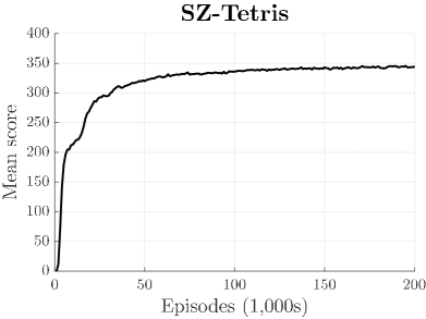
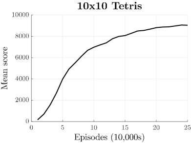
Figure 1: Average learning curves over the 12 algorithm instances in SZ-Tetris and in 10$\times$10 Tetris.

Figure 1 shows the average learning curves for the OMPAC method in SZ-Tetris and 10$\times$10 Tetris. The scores were computed as mean scores over every 10 generations (1,000 episodes) in SZ-Tetris and every 100 generations (10,000 episodes) in 10$\times$10 Tetris. The final scores are large and significant improvements of the previous state-of-the-art results achieved by shallow dSiL agents without OMPAC adaptation. The final average score of $345$ points is a $82$ points or $31\,\%$ improvement in SZ-Tetris, and the final average score of 9,000 points is a 4,100 points or $84\,\%$ improvement in 10$\times$10 Tetris.

Figure 2 shows the average values of the meta-parameters computed over the 12 algorithm instances.

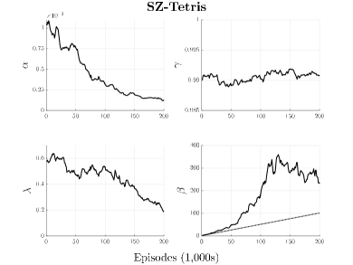
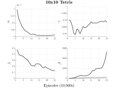
Figure 2: Average values of the meta-parameters in SZ-Tetris and 10$\times$10 Tetris for OMPAC adaptation. For visualization purposes, instead of showing $\tau(i)$, the figure shows the inverse temperature $\beta(i)=1/\tau(i)=(1+\tau_{k}i)/\tau_{0}$. The dotted lines in the $\beta$-panels show the $\beta(i)$-values for the starting values of $\tau_{0}$ and $\tau_{k}$.

The adaptations of $\alpha$ and $\lambda$ were similar in both games. The values of $\alpha$ decreased by about an order of magnitude, from $1.0{\times}10^{-3}$ to $1.25{\times}10^{-4}$ and $6.57{\times}10^{-5}$, and the values of $\lambda$ decreased from 0.55 to 0.188 and 0.125, in SZ-Tetris and in 10$\times$10 Tetris, respectively. More interestingly, while the value of $\gamma$ in SZ-Tetris was relatively stable around 0.99 (final average value of 0.9908), the value of $\gamma$ in 10$\times$10 Tetris first decreased to about 0.98 and then increased back towards 0.99 (final average value of 0.9886). The value of the inverse temperature $\beta=1/\tau$ in SZ-Tetris increased, in tandem with the improvement in mean score, to over 300 during first $\sim$125,000 episodes. During the last $\sim$75,000 episodes, there was only a very small ($\sim$5 points) improvement in mean score and the value of $\beta$ decreased slowly, reaching a final average value of 232. In 10$\times$10 Tetris, the mean score improved continuously and the value of $\beta$ increased over the whole learning process, reaching a final average value of $2670$ (i.e., approximately greedy action selection).

4.2 Atari 2600 games

We evaluated the OMPAC method in the Atari 2600 domain using the Arcade Learning Environment (Bellemare et al.,, 2013). We followed the experimental setup in our earlier study (Elfwing et al.,, 2017). The raw 210$\times$160 Atari 2600 RGB frames were pre-processed by extracting the luminance channel, taking the maximum pixel values over consecutive frames to prevent flickering, and then downsampling the grayscale images to 105$\times$80. The deep convolutional neural network used by the deep SiL agent consisted of two convolutional layers with SiL units (16 filters of size 8$\times$8 with a stride of 4 and 32 filters of size 4$\times$4 with a stride of 2), each followed by a max-pooling layer (pooling windows of size 3$\times$3 with a stride of 2), a fully-connected hidden layer with 512 dSiL units, and a fully-connected linear output layer with 4 to 18 output (or action-value) units, depending on the number of valid actions in the considered game. We used frame skipping where actions were selected every fourth frame and repeated for the next four frames. The input to the network was a 105$\times$80$\times$2 image consisting of the current and the fourth previous pre-processed frame. As in the DQN experiments (Mnih et al.,, 2015), we clipped the rewards to be between $-1$ and $+1$, but we did not clip the values of the TD-errors. An episode started with up to $30$ ’do nothing’ actions (no-op condition) and it was played until the end of the game or for a maximum of 18,000 frames (i.e., 5 minutes).

We used the meta-parameters in Elfwing et al., (2017) as starting values to initialize the meta-parameters according to Equations 15 and 16: $\alpha$: 0.001, $\gamma$: 0.99, $\lambda$: 0.8, $\tau_{0}$: 0.5, and $\tau_{k}$: 0.0005. The experiments ran for 2,000 generations (i.e., 200,000 episodes of learning in total). The score used for selection was the total raw score received by an algorithm instance in one generation.

The deep SiL agent in Elfwing et al., (2017) outperformed DQN, the Gorila implementation of DQN (Nair et al.,, 2015) and double DQN (van Hasselt et al.,, 2015) when tested on the 12 games played by DQN that started with the letters ’A’ and ’B’. In this study, we tested the OMPAC method in three Atari 2600 games: Alien, Amidar, and Assault. We choose those three because they are games where the deep SiL agents were outperformed by one or more of the other agents, and it should therefore be room for significant improvements in performance.

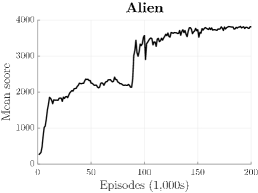
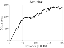
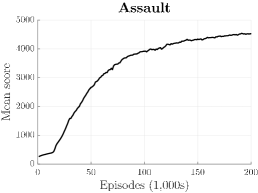
Figure 3: Average learning curves over the 12 algorithm instances in the Alien, Amidar, and Assault Atari 2600 games. The figure shows mean scores computed over every 10 generations (1,000 episodes).

Figure 3 shows the average learning curves over the 12 algorithm instances for the three games. Table 1 summarizes the results as the average scores in the final generation and the best mean scores of individual instances in any generation. The table also shows the final and best mean scores achieved by deep SiL agents without OMPAC adaptation, and the reported best mean scores achieved by DQN, the Gorila implementation of DQN, and double DQN. OMPAC adaptation of the meta-parameters significantly improved the performance of the deep SiL agents, between 83 % and 177 % when measured by average final scores and between 62 % and 82 % when measured by best mean scores. The OMPAC scores are also higher than the reported results for the other three methods, except for the double DQN score in the Assault game. However, the learned behavior in the Assault was still good. We tested the best performing agent in last generation using the final values of the meta-parameters, and it survived for the full 5 minutes in 88 out of 100 episodes. A video of a typical episode lasting for 5 minutes can be found at http://www.cns.atr.jp/~elfwing/videos/assault_OMPAC.mov.

Table 1: Average scores over the 12 instances in the final generations and the best mean scores of individual instances in any generation for deep SiL agents with OMPAC adaptation, final and best mean scores achieved by deep SiL agents without OMPAC adaptation, and the reported best mean scores achieved by DQN, the Gorila implementation of DQN, and double DQN in the no-op condition with 5 minutes of evaluation time.

				deep SiL		OMPAC
Game	DQN	Gorila	double DQN	Final	Best	Final	Best
Alien	3,069	2,621	2,907	1,370	2,246	3,798	4,097
Amidar	740	1,190	702	762	904	1,395	1,528
Assault	3,359	1,450	5,023	2,415	2,944	4,529	4,769

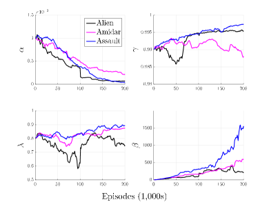
Figure 4: Average values of the meta-parameters in the Alien, Amidar, and Assault Atari 2600 games for OMPAC adaptation. For visualization purposes, instead of showing $\tau(i)$, the figure shows the inverse temperature $\beta(i)=1/\tau(i)=(1+\tau_{k}i)/\tau_{0}$.

Figure 4 shows average values of the meta-parameters over the learning process in the three Atari 2600 games. Similar to the two Tetris games, the values of $\alpha$ decreased, by about an order of magnitude of more, over the learning process. In contrast to the two Tetris games where the values of $\lambda$ decreased (from a smaller starting value of 0.55), the values of $\lambda$ either increased to about 0.9 (Amidar and Assault) or reached about 0.75 after first decreasing to 0.6 (Alien). The trajectories of the values of $\gamma$ and $\beta$ were different in the three games: 1) in Assault, both meta-parameters increased over the whole learning process (final average values of 0.9973 and 1556, for $\gamma$ and $\beta$, respectively); 2) in Amidar, the value of $\gamma$ was relatively stable but the value of $\beta$ increased, but slower than in Assault, over the whole learning process (0.9880 and 599); and 3) in Alien, the value of $\gamma$, similar to 10$\times$10 Tetris, decreased during the first $\sim$50,000 episodes before it started to increase, and the value of $\beta$, similar to SZ-Tetris, increased during the first $\sim$120,000 episodes when learning performance was increasing and it then slowly decreased when the learning performance plateaued (0.9953 and 206).

5 Analysis

In this section, we investigate the ability of the OMPAC method to learn when starting from bad settings of the meta-parameters. The experiments in the two Tetris and the Atari 2600 domains showed that OMPAC adaptation of the meta-parameters can significantly improve the learning performance when using suitable starting values of the meta-parameters. However, when, for example, encountering a new task, it would be valuable to be able to use OMPAC either as a method for achieving high performance even when the initial values of the meta-parameters are not suitable for the task at hand or as a method for finding suitable values of the meta-parameters for future experiments.

We chose to limit our investigation to different settings of $\gamma$ and $\tau_{k}$. We trained shallow dSiL agents in SZ-Tetris with three settings of the starting value of $\gamma\in\{0.8,0.9,0.99\}$ and three settings of the starting value of $\lambda\in\{$2.5$\times$10${}^{-3},$ 2.5$\times$10${}^{-4},$ 2.5$\times$10${}^{-5}\}$. We used the same values of the three other meta-parameters as in the earlier SZ-Tetris experiment. For each of the nine settings of $\gamma$ and $\tau_{k}$, we also trained agents without OMPAC adaptation for 10 separate runs.

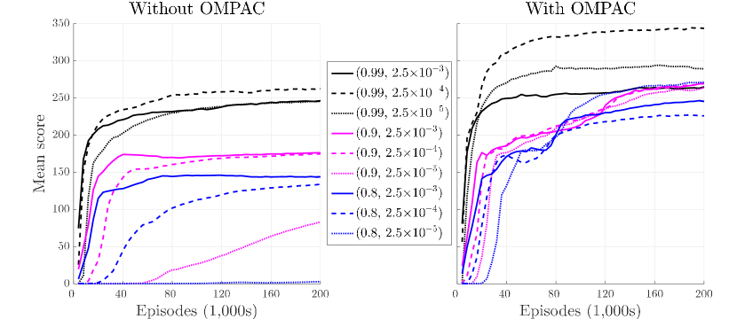
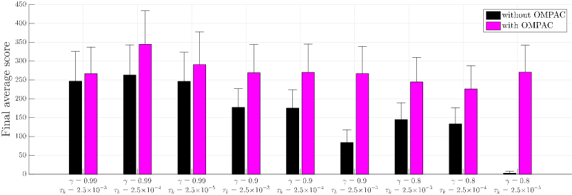
Figure 5: The top panel shows average learning curves for shallow dSiL agents in SZ-Tetris for different fixed values of $\gamma$ and $\tau_{k}$ (left) and for different starting values of the same meta-parameters for OMPAC adaptation (right). The three colors corresponds to different values of $\gamma$: black for 0.99, purple for 0.9, and blue for 0.8. The three line styles corresponds to different values of $\tau_{k}$: solid for 2.5$\times$10^-3, dashed for 2.5$\times$10^-4, dotted for 2.5$\times$10^-5. The bottom panel shows average scores over the final 1000 episodes with standard deviations

Figure 5 shows average learning curves with and without OMPAC adaptation of the meta-parameters (top panel), and the average scores over the final 1000 episodes with standard deviations (bottom panel). The results clearly show that the OMPAC method is able to overcome bad initial settings of meta-parameters. The two largest improvements in average final scores (267 and 183 points) were for the $(\gamma,\lambda)$-settings ((0.8, 2.5$\times$10^-5) and (0.9, 2.5$\times$10^-5)) that achieved the lowest average final scores (3 and 84 points) without OMPAC adaptation.

6 Conclusions

In this study, we proposed the OMPAC method for online adaptation of the meta-parameters in reinforcement learning by competition between algorithm instances running in parallel. We validated the proposed method by significantly improving the state-of-the-art scores in stochastic SZ-Tetris and 10$\times$10 Tetris, and by significantly improving the performance of deep Sarsa($\lambda$) agents in three Atari 2600 games. The experiments also demonstrated the ability of the OMPAC method to adapt the meta-parameters according to the learning progress in different tasks.

References

- Baker, (1987) Baker, J. E. (1987). Reducing bias and inefficiency in the selection algorithm. In Proceedings of the Second Genetic Algorithms on Genetic Algorithms and Their Application, pages 14–21.
- Bellemare et al., (2013) Bellemare, M. G., Naddaf, Y., Veness, J., and Bowling, M. (2013). The arcade learning environment: An evaluation platform for general agents. Journal of Artificial Intelligence Research, 47:253–279.
- Bertsekas and Ioffe, (1996) Bertsekas, D. P. and Ioffe, S. (1996). Temporal differences based policy iteration and applications in neuro-dynamic programming. Technical Report LIDS-P-2349, MIT.
- Burgiel, (1997) Burgiel, H. (1997). How to lose at Tetris. Mathematical Gazette, 81:194–200.
- Downey and Sanner, (2010) Downey, C. and Sanner, S. (2010). Temporal difference bayesian model averaging: A bayesian perspective on adapting lambda. In Proceedings of the International Conference on Machine Learning (ICML2010), pages 311–318.
- Elfwing et al., (2017) Elfwing, S., Uchibe, E., and Doya, K. (2017). Sigmoid-weighted linear units for neural network function approximation in reinforcement learning. CoRR, abs/1702.03118.
- Elfwing et al., (2008) Elfwing, S., Uchibe, E., Doya, K., and Christensen, H. I. (2008). Co-evolution of shaping rewards and meta-parameters in reinforcement learning. Adaptive Behavior, 16(6):400–412.
- Elfwing et al., (2011) Elfwing, S., Uchibe, E., Doya, K., and Christensen, H. I. (2011). Darwinian embodied evolution of the learning ability for survival. Adaptive Behavior, 19(2):101–120.
- Eriksson et al., (2003) Eriksson, A., Capi, G., and Doya, K. (2003). Evolution of meta-parameters in reinforcement learning algorithm. In Proceedings of the IEEE/RSJ Conference on Intelligent Robots and Systems (IROS2003), pages 412–417.
- Faußer and Schwenker, (2013) Faußer, S. and Schwenker, F. (2013). Neural network ensembles in reinforcement learning. Neural Processing Letters, pages 1–15.
- François-Lavet et al., (2015) François-Lavet, V., Fonteneau, R., and Ernst, D. (2015). How to discount deep reinforcement learning: Towards new dynamic strategies. CoRR, abs/1512.02011.
- Gabillon et al., (2013) Gabillon, V., Ghavamzadeh, M., and Scherrer, B. (2013). Approximate dynamic programming finally performs well in the game of Tetris. In Proceedings of Advances in Neural Information Processing Systems (NIPS2013), pages 1754–1762.
- Ishii et al., (2002) Ishii, S., Yoshida, W., and Yoshimoto, J. (2002). Control of exploitation–exploration meta-parameter in reinforcement learning. Neural Networks, 15(4-6):665–687.
- Kobayashi et al., (2009) Kobayashi, K., Mizoue, H., Kuremoto, T., and Obayashi, M. (2009). A meta-learning method based on temporal difference error. In Proceedings of International Conference on Neural Information Processing (ICONIP2009), pages 530–537.
- Lamarck, (1809) Lamarck, J. B. (1809). Philosophie Zoologique. Chez Dentu.
- Mann et al., (2016) Mann, T. A., Penedones, H., and Hester, T. (2016). Adaptive least-squares temporal difference learning. CoRR, abs/1612.09465.
- Mnih et al., (2015) Mnih, V., Kavukcuoglu, K., Silver, D., Rusu, A. A., Veness, J., Bellemare, M. G., Graves, A., Riedmiller, M., Fidjeland, A. K., Ostrovski, G., Petersen, S., Beattie, C., Sadik, A., Antonoglou, I., King, H., Kumaran, D., Wierstra, D., Legg, S., and Hassabis, D. (2015). Human-level control through deep reinforcement learning. Nature, 518(7540):529–533.
- Nair et al., (2015) Nair, A., Srinivasan, P., Blackwell, S., Alcicek, C., Fearon, R., Maria, A. D., Panneershelvam, V., Suleyman, M., Beattie, C., Petersen, S., Legg, S., Mnih, V., Kavukcuoglu, K., and Silver, D. (2015). Massively parallel methods for deep reinforcement learning. CoRR, abs/1507.04296.
- Rummery and Niranjan, (1994) Rummery, G. A. and Niranjan, M. (1994). On-line Q-learning using connectionist systems. Technical Report CUED/F-INFENG/TR 166, Cambridge University Engineering Department.
- Schweighofer and Doya, (2003) Schweighofer, N. and Doya, K. (2003). Meta-learning in reinforcement learning. Neural Networks, 16(1):5–9.
- Sutton, (1988) Sutton, R. S. (1988). Learning to predict by the method of temporal differences. Machine Learning, 3:9–44.
- Sutton, (1992) Sutton, R. S. (1992). Adapting bias by gradient descent: an incremental version of the delta-bar-delta. In Proceedings of the National Conference on Artificial Intelligence.
- Sutton, (1996) Sutton, R. S. (1996). Generalization in reinforcement learning: Successful examples using sparse coarse coding. In Proceedings of Advances in Neural Information Processing Systems (NIPS1996), pages 1038–1044. MIT Press.
- Sutton and Barto, (1998) Sutton, R. S. and Barto, A. (1998). Reinforcement Learning: An Introduction. MIT Press.
- Szita and Szepesvári, (2010) Szita, I. and Szepesvári, C. (2010). SZ-Tetris as a benchmark for studying key problems of reinforcement learning. In ICML 2010 workshop on machine learning and games.
- Unemi et al., (1994) Unemi, T., Nagaoyoshi, M., Hirayama, N., Nade, T., Yano, K., and Masujima, Y. (1994). Differentiation of learning abilities – a case study on optimizing parameter values in q-learning by a genetic algorithm. In Proceedings of the International Workshop on the Synthesis and Simulation of Living Systems, pages 331–336.
- van Hasselt et al., (2015) van Hasselt, H., Guez, A., and Silver, D. (2015). Deep reinforcement learning with double q-learning. CoRR, abs/1509.06461.