Speckle Reduction with Trained Nonlinear Diffusion Filtering

Abstract

Speckle reduction is a prerequisite for many image processing tasks in synthetic aperture radar (SAR) images, as well as all coherent images. In recent years, predominant state-of-the-art approaches for despeckling are usually based on nonlocal methods which mainly concentrate on achieving utmost image restoration quality, with relatively low computational efficiency. Therefore, in this study we aim to propose an efficient despeckling model with both high computational efficiency and high recovery quality. To this end, we exploit a newly-developed trainable nonlinear reaction diffusion(TNRD) framework which has proven a simple and effective model for various image restoration problems. In the original TNRD applications, the diffusion network is usually derived based on the direct gradient descent scheme. However, this approach will encounter some problem for the task of multiplicative noise reduction exploited in this study. To solve this problem, we employed a new architecture derived from the proximal gradient descent method. Taking into account the speckle noise statistics, the diffusion process for the despeckling task is derived. We then retrain all the model parameters in the presence of speckle noise. Finally, optimized nonlinear diffusion filtering models are obtained, which are specialized for despeckling with various noise levels. Experimental results substantiate that the trained filtering models provide comparable or even better results than state-of-the-art nonlocal approaches. Meanwhile, our proposed model merely contains convolution of linear filters with an image, which offers high level parallelism on GPUs. As a consequence, for images of size $512\times 512$, our GPU implementation takes less than 0.1 seconds to produce state-of-the-art despeckling performance.

1 Introduction

Synthetic aperture radar (SAR) images are inevitably corrupted by speckle noise, due to constructive and destructive electromagnetic wave interference during image acquisition. With fleets of satellites delivering a huge number of images, automatic analysis tools are essential for remote sensing major applications. Therefore, the quality of source images should be sufficient such that it is easy to extract information. However, the speckle noise visually degrades the appearance of images and therefore hinders automatic scene analysis and information extraction [6, 20]. For instance, speckle is the main obstacle towards the development of an effective optical-SAR fusion [4]. Hence, speckle reduction is a necessary preprocessing step in SAR image processing. Despeckling techniques have been extensively studied for almost 30 years [33, 31], and new algorithms are continuously proposed to provide better and better performance. Up to now, the despeckling techniques fall broadly into four categories: filtering based methods in (1) spatial domain or (2) a transform domain, e.g., wavelet domain; (3) nonlocal filtering; and (4) variational methods. As a comprehensive review of the despeckling algorithms is beyond the scope of this paper, we only provide a brief introduction for these methods. For more details, we refer the reader to [6].

The multi-look technique is a traditional spatial approach. It amounts to incoherently averaging independent observations of the same resolution cell, thus reducing the noise intensity. However, this simple averaging approach results in a clear loss in image resolution. To overcome this deficiency, a great deal of research has been conducted to develop suitable spatial filters which can reduce the noise, yet preserve details and edges [26] [37]. Filters of this kind include Lee filter proposed in [33] [34] which was developed under the minimum-mean-square-error (MMSE) criterion, and Kuan filter [31] as well as the $\Gamma$-Map filter [36] which are based on the more sophisticated maximum a posteriori (MAP) approach.

Anisotropic diffusion [43] based method is also a type of widely exploited spatial filtering technology for despeckling. Anisotropic diffusion is a popular technique in the image processing community, that aims at reducing image noise without removing significant parts of the image content. A few related works that apply anisotropic diffusion filtering for the despeckling task include speckle reducing anisotropic diffusion (SRAD) [53] and detail preserving anisotropic diffusion (DPAD) [3]. SRAD exploits the instantaneous coefficient of variation and it leads to better performance than the conventional anisotropic diffusion method in terms of mean preservation, variance reduction and edge localization. DPAD modifies the SRAD filter to rely on the Kuan filter [31] rather than the Lee filter. DPAD estimates the local statistics using a larger neighborhood, instead of the four direct neighbors used by SRAD. However, the despeckling methods based on anisotropic diffusion fell out of favor in recent years mainly because of limited performance. It is clear that there is a despeckling quality gap between the diffusion based approaches and state-of-the-art nonlocal algorithms.

Image filtering in the domain of wavelet has also been widely exploited for despeckling. Most of the wavelet-based despeckling techniques employ the statistical wavelet shrinkage technique with MAP Bayesian approach, e.g.[44, 1, 8, 45, 5]. In general, the wavelet-based methods guarantee a superior ability to preserve signal resolution in comparison with conventional spatial filters. However, they often suffer from isolated patterns in flat areas, or ringing effects near the edges of the images, leading to visually unappealing results.

Recently, incorporation with the modern denoising methods, e.g., nonlocal mean (NLM) [10], block-matching 3-D (BM3D) [17] and K-SVD [23], several nonlocal despeckling approaches have been proposed [18], [50], [42], [29]. Originated from the NLM algorithm, the probabilistic patch-based (PPB) filter [18] provides promising results by developing an effective similarity measure well suited to SAR images. A drawback of the PPB filter is the suppression of thin and dark details in the regularized images. As an extension of BM3D, Parrilli $et$ $al.$ [42] derived a SAR-oriented version of BM3D by taking into account the peculiar features of SAR images. It exhibits an objective performance comparable or superior to other techniques on simulated speckled images, and guarantees a very good subjective quality on real SAR images. Typical artifacts of the nonlocal methods are in the form of structured signal-like patches in flat areas, originated from the randomness of speckle and reinforced through the patch selection process. Generally speaking, most of these techniques mainly concentrate on achieving utmost despeckling quality, with relatively low computational efficiency. An notable exception is BM3D with its improved version [15]. However, the BM3D-based method involves a block matching process, which is challenging for parallel computation on GPUs, alluding to the fact that it is not straightforward to accelerate BM3D algorithm on parallel architectures.

The fourth category, i.e., variational methods [48, 7, 25, 12, 22, 30, 11, 24, 21, 28], minimizes some appropriate energy functionals consisted of an image prior regularizer and a data fitting term. As a well-known regularizer, total variation (TV) has been widely used for the despeckling task [48, 7, 21, 28]. For instance, in [21] a new variational model based on a hybrid data term and the widely used TV regularizer is proposed for restoring blurred images with multiplicative noise. Moreover, [28] proposes a two-step approach to solve the problem of restoring images degraded by multiplicative noise and blurring, where the multiplicative noise is first reduced by nonlocal filters and then a convex variational model is adopted to obtain the final restored images. Solutions of variational problems with TV regularization admit many desirable properties, most notably the appearance of sharp edges.

However, TV-based methods generate the so-called staircasing artifact. To remedy the staircasing artifact, [25] incorporates the total generalized variation (TGV) [9] penalty into the existing data fidelity term for speckle removal, and develops two novel variation despeckling models. By involving and balancing higher-order derivatives of the image, the TGV-based despeckling method outperforms the traditional TV methods by reducing the staircasing artifact. Recently, different from hand-crafted regularizers, such as TV and TGV models, [12] proposes a novel variational approach for speckle removal, which combines an image prior model named Fields of Experts (FoE) [46] and a recently proposed efficient non-convex optimization algorithm - iPiano [40]. The proposed method in [12] can obtain strongly competitive despeckling performance w.r.t. the state-of-the-art method - SAR-BM3D, meanwhile, preserve the property of computational efficiency.

1.1 Our Contribution

Traditional despeckling approaches based on anisotropic diffusion are handcrafted models which include elaborate selections of diffusivity coefficient, or optimal stopping time or proper reaction force term. In order to improve the capacity of the traditional diffusion-based despeckling models, we employ the newly-developed anisotropic diffusion based model [13] with trainable filters and influence functions. Instead of the first order gradient operator in previous diffusion-based despeckling models, we explore more filters of larger kernel size targeted for despeckling. On the other hand, different influence functions are considered and trained for different filters, rather than an unique function in the traditional diffusion model. Moreover, the parameters of each iteration can vary across diffusion steps.

As shown in [13], the optimized nonlinear diffusion model has broad applicability to a variety of image restoration problems, and achieves recovery results of high quality surpassing recent state-of-the-arts. Furthermore, it only involves a small number of explicit filtering steps, and hence is highly computationally efficient, especially with parallel computation on GPUs.

In this paper, we intend to apply the TNRD framework [13] to the task of multiplicative noise reduction. However, a direct use of the original TNRD model is not feasible, as we have to make a few modifications oriented to this specific task:

• We need to redesign the diffusion process by taking into consideration the peculiarity of multiplicative noise statistics.

• Based on the new diffusion process specialized for multiplicative noise reduction, we need to recalculate the gradients required for the training phase.

• In the original TNRD applications, the diffusion network is usually derived based on the direct gradient descent scheme. However, this approach will encounter some problem for the task of multiplicative noise reduction exploited in this work. The reason is explained in detail in Section 3.1 and the experimental part 4.1. To solve this problem, we employed a new architecture as shown in Fig. 2, which is derived from the proximal gradient descent method. Comparing Fig. 2 and Fig. 1, we can see that the structure of the proposed diffusion process Fig. 2 in our study is quite different from the original TNRD model Fig. 1.

Then, the model parameters in the diffusion process need to be trained by taking into account the Speckle noise statistics, including the linear filters and influence functions. Eventually, we reach a nonlinear reaction diffusion based approach for despeckling, which leads to state-of-the-art performance, meanwhile gains high computationally efficiency. Experimental results show that the proposed despeckling approach with optimized nonlinear diffusion filtering leads to state-of-the-art performance, meanwhile gains high computationally efficiency.

1.2 Organization

The remainder of the paper is organized as follows. Section II presents a general review of the speckle noise and the trainable nonlinear reaction diffusion process, which is required to derive the optimized diffusion process for despeckling. In the subsequent section III, we propose the optimized nonlinear diffusion process for despeckling. Subsequently, Section IV describes comprehensive experiment results for the proposed model. The concluding remarks are drawn in the final Section V.

2 Preliminaries

To make the paper self-contained, in this section we provide a brief review of the statistics property of speckle noise and the trainable nonlinear diffusion process proposed in [13].

2.1 Speckle Noise

Assume that $f\in\mathbb{R}^{N}$ (represented as a column-stacked vector) denotes the observed SAR image amplitude with number of looks $L$, and $u\in\mathbb{R}^{N}$ denotes the underlying true image amplitude i.e., the square root of the reflectivity. According to [27] [6], the fully-developed speckle can be modeled as the multiplicative Goodman’s noise, i.e.,

$$f=un,$$ (2.1)

where $n$ is the so-called speckle noise. In the multiplicative, or fully-developed, speckle model, the conditional pdf of $f$ given $u$ follows a Nakagami distribution:

$$p(f|u)=\frac{2L^{L}}{\Gamma(L)u^{2L}}f^{2L-1}\text{exp}\left(-\frac{Lf^{2}}{u^{2}}\right)\,,$$

where $\Gamma$ is the classical Gamma function. Note that the distribution According to the Gibbs function, this likelihood leads to the following energy term via $E=-\text{log}p(f|u)$

$$D_{1}(u,f)=\langle L\cdot(2\text{log}u+\frac{f^{2}}{u^{2}}),1\rangle\,,$$ (2.2)

where $\langle,\rangle$ denotes inner product. Unfortunately, this term is nonconvex w.r.t. $u$, that is cumbersome to derive the diffusion process as described in Sec. 3.1. There are two ways to resolve the nonconvexity. First, logarithmic transformation (i.e., $u_{l}=\text{log}\left(u\right)$) can be used. The resulting energy term is expressed as follows:

$$D_{2}(u_{l},f)=\langle L\cdot(2u_{l}+{f^{2}}{e^{-2u_{l}}}),1\rangle\,.$$ (2.3)

Second, an alternative method to define a convex date term is using the classical Csiszár I-divergence model [16], which is typically derived for Poisson noise. The I-divergence based data term for the amplitude model is given by [48, 25]

$$D_{3}(u,f)=\langle\lambda(u^{2}-2f^{2}\text{log}u),1\rangle\,,$$ (2.4)

which is strictly convex w.r.t. $u$.

Concerning the relation between (2.2) and (2.4), by following the argument stated in Steidl and Teuber’s work [48], we achieve similar equivalence by incorporating these two data terms into a Total Variation (TV) regularized variational model in the continuous form. The derivation reads as follows. Regarding the data term (2.2), let us consider the following convex variational functional by setting $u=e^{\frac{1}{2}w}$

$$\hat{w}=\arg\min\limits_{w\in BV}\int_{\Omega}\left(w+f^{2}e^{-w}\right)dx+\lambda|w|_{TV},~{}\hat{u}=e^{\frac{1}{2}\hat{w}}\,,$$ (2.5)

where $|w|_{TV}$ is the TV semi-norm defined as

$$|w|_{TV}=\int_{\Omega}|\nabla w|dx\,.$$ (2.6)

Regarding the data term (2.2), let us consider the following convex variational functional by setting $u=\sqrt{v}$

$$\hat{v}=\arg\min\limits_{v\in BV,v>0}\int_{\Omega}\left(v-f^{2}\text{log}v\right)dx+\lambda|v|_{TV},~{}\hat{u}=\sqrt{v}\,.$$ (2.7)

As $\nabla e^{w}=e^{w}\nabla w$, we have for $u=e^{w}$ that $\nabla u(x)=0$ if and only if $\nabla w(x)=0$. As a consequence, if we minimize (2.5) and (2.7) over smooth functions, the minimizer $\hat{w}$ for (2.5) and the minimizer $\hat{v}$ for (2.7) are respectively given by

$$1-f^{2}e^{-\hat{w}}-\lambda\text{div}\frac{\nabla\hat{w}}{|\nabla\hat{w}|}=0\,,$$

and

$$1-\frac{f^{2}}{\hat{v}}-\lambda\text{div}\frac{\nabla\hat{v}}{|\nabla\hat{v}|}=0\,,$$

for those points $|\nabla\hat{w}(x)|\neq 0$ and $|\nabla\hat{v}(x)|\neq 0$. Since we have $\frac{\nabla w}{|\nabla w|}=\frac{e^{w}\nabla w}{e^{w}|\nabla w|}=\frac{\nabla u}{|\nabla u|}$, it turns out that the minimizer $\hat{w}$ and $\hat{v}$ of the functional in the model (2.5) and model (2.7) respectively, coincide in the sense that $\hat{v}=e^{\hat{w}}$. Therefore, for both $\hat{u}$, we will obtain the same result. Note that this conclusion only holds for the those $L_{1}$-norm induced regularizers, such as the TV regularization. For some other regularized variational models (e.g., TGV-based model [25]), although this data term (2.4) seems inappropriate, it performs very well for despeckling.

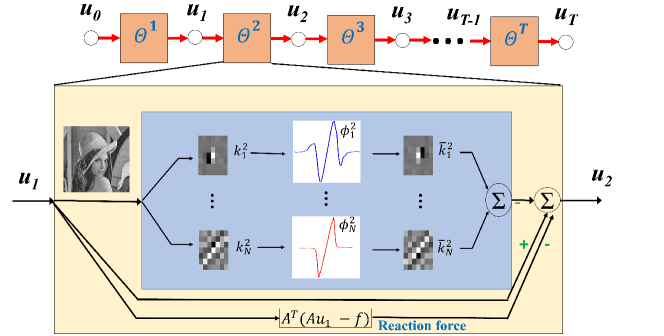
Figure 1: The detailed architecture of the original TNRD model with a reaction term, e.g., $\psi(u_{t-1},f)=A^{\top}(Au_{t-1}-f)$. Note that it is represented as a feed-forward network.

2.2 Trainable Nonlinear Reaction Diffusion (TNRD)

2.2.1 Highly parametrized nonlinear diffusion model

Recently, a simple but effective framework for image restoration called TNRD was proposed in [13], which is based on the concept of nonlinear reaction diffusion. The TNRD framework is modeled by highly parametrized linear filters as well as highly parametrized influence functions. In contrast to those conventional nonlinear diffusion models which usually make use of handcrafted parameters, all the parameters in the TNRD model, including the filters and the influence functions, are learned from training data through a loss based approach.

The proposed framework is formulated as the following time-dynamic nonlinear reaction-diffusion process with $T$ steps

$$\footnotesize\begin{cases}u_{0}=I_{0},\quad t=1\cdots T\\ u_{t}=\underbrace{\text{Prox}_{\mathcal{G}^{t}}}_{\text{reaction force}}\left(u_{t-1}-\left(\underbrace{\sum\limits_{i=1}^{N_{k}}\bar{k}_{i}^{t}*\phi_{i}^{t}(k_{i}^{t}*u_{t-1})}_{\text{diffusion force}}+\underbrace{\psi^{t}(u_{t-1},f)}_{\text{reaction force}}\right)\right)\,,\end{cases}$$ (2.8)

where $I_{0}$ is the initial status of the diffusion process, $*$ is the convolution operation, $T$ denotes the diffusion stages, $N_{k}$ denotes the number of filters, $k_{i}^{t}$ are time varying convolution kernels, $\bar{k}_{i}$ is obtained by rotating the kernel $k_{i}$ 180 degrees, $k_{i}*u$ denotes 2D convolution of the image $u$ with the filter kernel $k_{i}$, and $\phi_{i}^{t}$ are time varying influence functions (not restricted to be of a certain kind). Both the proximal mapping operation $\text{Prox}_{\mathcal{G}^{t}}(\hat{u})$ and $\psi^{t}(u_{t},f)$ are the reaction force. Usually, the reaction term $\psi^{t}(u)$ is chosen as the derivative of a certain smooth date term $\mathcal{D}(u,f)$, i.e., $\psi^{t}(u)=\nabla_{u}\mathcal{D}^{t}(u)$. Note that the proximal mapping operation [39] related to the function $\mathcal{G}^{t}$ is given as

$$\text{Prox}_{\mathcal{G}^{t}}(\hat{u})=\min\limits_{u}\frac{\|u-\hat{u}\|_{2}^{2}}{2}+\mathcal{G}^{t}(u,f)\,.$$

As shown in [13], the proposed model (2.8) can be interpreted as performing one gradient descent step at $u^{t}$ with respect to a dynamic energy functional given by

$$E^{t}(u,f)=\sum\limits_{i=1}^{N_{k}}\sum\limits_{p=1}^{N}\rho_{i}^{t}((k_{i}^{t}*u)_{p})+\mathcal{D}^{t}(u,f)+\mathcal{G}^{t}(u,f)\,,$$ (2.9)

where the functions $\left\{\rho_{i}^{t}\right\}_{t=0}^{t=T-1}$ are the so-called penalty functions and the regularization parameter is included in $\mathcal{D}^{t}(u,f)$. Note that $\rho^{\prime}(z)=\phi(z)$ and the parameters {$k_{i}^{t},\rho_{i}^{t}$} vary across the stages i.e., changes at each iteration.

It is easy to apply the proposed TRND framework to different image restoration problems by incorporating specific reaction force, such as Gaussian denoising, image deblurring, image super resolution and image inpainting. This is realized by setting $\mathcal{G}^{t}=0$, while $\mathcal{D}^{t}(u,f)=\frac{\lambda^{t}}{2}\|Au-f\|_{2}^{2}$ and $\psi^{t}(u)=\lambda^{t}A^{\top}(Au-f)$, where $\lambda^{t}$ is related to the strength of the reaction term, $u$ and $f$ denote the original true image and the input degraded image, respectively, and $A$ is the associated different linear operator. In the case of Gaussian denoising, $A$ is the identity matrix; for image super resolution, $A$ is related to the down sampling operation and for image deconvolution, $A$ should correspond to the linear blur kernel.

2.2.2 Overall training scheme

The proposed diffusion model in [13] is trained in a supervised manner. In other words, the input/output pairs for certain image processing task are firstly prepared, and then we exploit a loss minimization scheme to optimize the model parameters $\Theta^{t}$ for each stage $t$ of the diffusion process. The training dataset consists of $S$ training samples $\{u_{gt}^{s},f^{s}\}_{s=1}^{S}$, where $u_{gt}^{s}$ is a ground truth image and $f^{s}$ is the corresponding degraded input. The model parameters in stage $t$ required to be trained include 1) the reaction force weight $\lambda$, (2) linear filters and (3) influence functions. All parameters are grouped as $\Theta^{t}$, i.e., $\Theta^{t}=\{\lambda^{t},\phi_{i}^{t},k_{i}^{t}\}$. Then, the optimization problem for the training task is formulated as follows

$$\small\begin{cases}\min\limits_{\Theta}\mathcal{L}(\Theta)=\sum\limits_{s=1}^{S}\ell(u_{T}^{s},u_{gt}^{s})=\sum\limits_{s=1}^{S}\frac{1}{2}\|u_{T}^{s}-u_{gt}^{s}\|^{2}_{2}\\ \text{s.t.}\begin{cases}u_{0}^{s}=I_{0}^{s}\\ u_{t}^{s}=\text{Prox}_{\mathcal{G}^{t}}\left(u_{t-1}^{s}-\left({\sum\limits_{i=1}^{N_{k}}\bar{k}_{i}^{t}*\phi_{i}^{t}(k_{i}^{t}*u_{t-1}^{s})}+\psi^{t}(u_{t-1}^{s},f^{s})\right)\right),\\ t=1\cdots T\,,\end{cases}\end{cases}$$ (2.10)

where $\Theta=\{\Theta^{t}\}_{t=1}^{t=T}$. The training problem in (2.10) can be solved via gradient based algorithms, e.g., the L-BFGS algorithm [35], where the gradients associated with $\Theta_{t}$ are computed using the standard back-propagation technique [32].

There are two training strategies to learn the diffusion processes: 1) the greedy training strategy to learn the diffusion process stage-by-stage; and 2) the joint training strategy to train a diffusion process by simultaneously tuning the parameters in all stages. Generally speaking, the joint training strategy performs better [13], and the greedy training strategy is often used to provide a good initialization for the joint training. Concerning the joint training scheme, the gradients $\frac{\partial\ell(u_{T},u_{gt})}{\partial\Theta_{t}}$ are computed as follows,

$$\frac{\partial\ell(u_{T},u_{gt})}{\partial\Theta_{t}}=\frac{\partial u_{t}}{\partial\Theta_{t}}\cdot\frac{\partial u_{t+1}}{\partial u_{t}}\cdots\frac{\partial\ell(u_{T},u_{gt})}{\partial u_{T}}\,.$$ (2.11)

For different image restoration problems, we mainly need to recompute the two components $\frac{\partial u_{t}}{\partial\Theta_{t}}$ and $\frac{\partial u_{t+1}}{\partial u_{t}}$, the main part of which are similar to the derivations in [13].

3 Optimized Nonlinear Diffusion Filtering for Despeckling

3.1 Proposed Trainable Reaction Diffusion Filtering for Despeckling

The diffusion filtering process for despeckling can be derived from the energy functional (2.9) by incorporating data fidelity terms in (2.2)-(2.4).

Considering the data term (2.3), we have the following energy functional

$$E(w,f)=\sum\limits_{i=1}^{N_{k}}\sum\limits_{p=1}^{N}\rho_{i}((k_{i}*e^{w})_{p})+\lambda\langle 2w+f^{2}e^{-2w},1\rangle\,,$$ (3.1)

with $u=e^{w}$. Then, we derive the corresponding diffusion process by setting $\mathcal{D}(w,f)=\lambda\langle 2w+f^{2}e^{-2w},1\rangle$ and $\mathcal{G}=0$, as the proximal mapping operation w.r.t $\mathcal{G}(w,f)=\lambda\langle 2w+f^{2}e^{-2w},1\rangle$ is not easy to compute. The resulting diffusion process is given as

$$w_{t}=w_{t-1}-\left(\begin{array}[]{l}\sum\limits_{i=1}^{N_{k}}e^{w_{t-1}}\odot\left(\bar{k}_{i}^{t}*\phi_{i}^{t}(k_{i}^{t}*e^{w_{t-1}})\right)+{\lambda^{t}}(2-2f^{2}e^{-2w_{t-1}})\end{array}\right)\,,$$

where $\odot$ denotes element-wise product. However, due to the formulation $e^{w_{t-1}}\odot\left(\bar{k}_{i}^{t}*\phi_{i}^{t}(k_{i}^{t}*e^{w_{t-1}})\right)$, the value of $e^{w_{T}}$ is prone to explosion in training phase and therefore makes the training fail.

If we consider the data term (2.2), we arrive at the following energy functional

$$E(u,f)|_{u>0}=\sum\limits_{i=1}^{N_{k}}\sum\limits_{p=1}^{N}\rho_{i}((k_{i}*u)_{p})+\lambda\langle 2\text{log}u+\frac{f^{2}}{u^{2}},1\rangle\,.$$ (3.2)

As the proximal mapping operator $\text{Prox}_{\mathcal{G}}(\cdot)$ only works for a convex function $\mathcal{G}$, we have to set $\mathcal{D}(u,f)=\lambda\langle 2\text{log}u+\frac{f^{2}}{u^{2}},1\rangle$ and $\mathcal{G}=0$ in (2.9). Then we arrive at a direct gradient descent process with ${\psi(u_{t},f)}=\lambda\left(\frac{2}{u}-\frac{2f^{2}}{u^{3}}\right)$. However, this straightforward gradient descent approach is not applicable in practice, because (1) at the points with $u$ very close to zero the reaction term is enlarged so much that there will be an obvious problem of numerical instability; (2) this update rule may produce negative values of $u$ after one diffusion step, which will violate the constraint of the data term in (3.2).

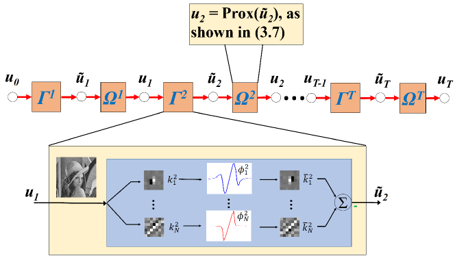
Figure 2: The architecture of the proposed diffusion model for despeckling. It is represented as a feed-forward network. Note that the additional convolution step with the rotated kernels $\bar{k}_{i}$. Here, the training parameters for the $t$th step are $\mathit{\Theta}^{t}=\left\{\mathit{\Gamma}^{t},\mathit{\Omega}^{t}\right\}$ with $\mathit{\Gamma}^{t}=\{\phi_{i}^{t},k_{i}^{t}\}_{i=1}^{N_{k}}$ and $\mathit{\Omega}^{t}=\lambda^{t}$ respectively. More importantly, the employed scheme based on the proximal gradient descent method is quite different from the straightforward direct gradient descent (as shown in Fig. 1) employed for TNRD-based denoisng task [14].

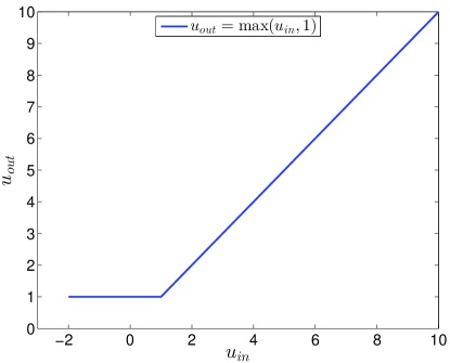
Figure 3: The hard shrinkage operation $u_{out}=\mathrm{max}(u_{in},c)$ with $c=1$.

In order to remedy the aforementioned problems, after each diffusion step, we additionally consider a simple projection operation

$$u=\max(\tilde{u},c),~{}\text{with}~{}c>0\,,$$

to shrink those “bad” pixels, which do not satisfy the constraint $u>0$ or are very close to zero. Therefore, we arrive at the following diffusion approach

$$\begin{split}\tilde{u}_{t+1}&=u_{t}-\left(\sum\limits_{i=1}^{N_{k}}\bar{k}_{i}^{t+1}*\phi_{i}^{t+1}(k_{i}^{t+1}*u_{t})+\frac{\lambda^{t+1}}{u_{t}}\left(1-\frac{f^{2}}{u_{t}^{2}}\right)\right)\,,\\ {u}_{t+1}&=\max(\tilde{u}_{t+1},c)\,.\end{split}$$ (3.3)

An illustrative example of the shrinkage function related to the projection operation is show in Fig. 3, where we set $c=1$. Note that as the shrinkage function is differentiable, it is not problematic in the training phase.

As the projection operation will somehow manipulate the pixel values, a small $c$ is required to reduce its influence. However, on the other hand, a small $c$ will raise a problem of numerical stability due to the formulation $\frac{2}{u}-\frac{2f^{2}}{u^{3}}$, and then training will fail. In order to search an appropriate $c$ for our diffusion model, we progressively increased $c$ from $0.1$ with four settings $c=0.1,0.2,0.5,\text{and}~{}1$. We observed that the former three settings led to failure in the training phase, and $c=1$ is sufficient for a stable training.

However, although the diffusion model (3.3) overcomes the shortcomings of the model (2.2), it encounters some other problems which will be explained in detail in the experimental part 4.1.

As a consequence, we resort to the data term (2.4). Although the data term (2.4) sounds inappropriate, it is incorporated in a flexible training framework with many free parameters. The training phase can somehow automatically adapt to this inappropriate data term.

Therefore, we exploit the data term (2.4), and reach the following energy functional

$$\min\limits_{u>0}E(u)=\sum\limits_{i=1}^{N_{k}}\sum\limits_{p=1}^{N}\rho_{i}((k_{i}*u)_{p})+\lambda\langle u^{2}-2f^{2}\text{log}u,1\rangle\,.$$ (3.4)

As the data term in (3.4) is smooth and differentiable we have two possible ways to derive the diffusion process.

• By setting $\mathcal{D}(u,f)=\lambda\left\langle u^{2}-2f^{2}\text{log}u,1\right\rangle$ and $\mathcal{G}=0$ in (2.9), we arrive at a direct gradient descent process with ${\psi(u_{t},f)}=\lambda\left(2u-\frac{2f^{2}}{u}\right)$. In this case, we will encounter the same problem mentioned above, thus intractable in practice.

• By setting $\mathcal{D}=0$ and $\mathcal{G}(u,f)=\lambda\left\langle u^{2}-2f^{2}\text{log}u,1\right\rangle$ in (2.9), the resulting diffusion process is able to overcome the above shortcomings. Details read as follows.

Recall that the proximal mapping with respect to $\mathcal{G}$ is given as the following minimization problem

$$\left(\mathbf{I}+\partial\mathcal{G}\right)^{-1}(\tilde{u})=\arg\min\limits_{u}\frac{\|u-\tilde{u}\|^{2}_{2}}{2}+\lambda\langle u^{2}-2f^{2}\mathrm{log}u,1\rangle\,.$$ (3.5)

The solution of (3.5) is given by the following point-wise operation

$$\hat{u}=\left(\mathbf{I}+\partial\mathcal{G}\right)^{-1}(\tilde{u})=\frac{\tilde{u}+\sqrt{\tilde{u}^{2}+8\left(1+2\lambda\right)\lambda f^{2}}}{2\left(1+2\lambda\right)}\,.$$ (3.6)

Note that this update rule is able to guarantee $\hat{u}>0$ in diffusion steps because $\hat{u}$ is always positive if $f>0$.

Finally, the diffusion process for despeckling using the proximal gradient method is formulated as

$$u_{t+1}=\frac{\tilde{u}_{t+1}+\sqrt{\tilde{u}_{t+1}^{2}+8\left(1+2\lambda^{t+1}\right)\lambda^{t+1}f^{2}}}{2\left(1+2\lambda^{t+1}\right)}\,,$$ (3.7)

where $\tilde{u}_{t+1}=u_{t}-\sum\limits_{i=1}^{N_{k}}\bar{k}_{i}^{t+1}*\phi_{i}^{t+1}(k_{i}^{t+1}*u_{t})$. The architecture of the proposed diffusion model for despeckling is as shown in Fig. 1.

3.2 Computing The Gradients for Training

In this section we derive the gradients of the loss function w.r.t the training parameters $\Theta_{t}=\left\{\lambda^{t},\phi_{i}^{t},k_{i}^{t}\right\}$ in joint training. In summary, we need to compute three parts of $\frac{\partial\ell(u_{T},u_{gt})}{\partial\Theta_{t}}$, i.e., $\frac{\partial u_{t+1}}{\partial u_{t}}$, $\frac{\partial u_{t}}{\partial\Theta_{t}}$ and $\frac{\partial\ell(u_{T},u_{gt})}{\partial u_{T}}$.

First of all, according to (2.10), it is easy to check that the gradient $\frac{\partial\ell(u_{T},u_{gt})}{\partial u_{T}}$ is given as follows

$$\frac{\partial\ell(u_{T},u_{gt})}{\partial u_{T}}=u_{T}-u_{gt}\,,$$

where we omit the image index $s$ for brevity. Then, $\frac{\partial u_{t+1}}{\partial u_{t}}$ is computed as follows according to the chain rule,

$$\frac{\partial u_{t+1}}{\partial u_{t}}=\frac{\partial\tilde{u}_{t+1}}{\partial u_{t}}\cdot\frac{\partial u_{t+1}}{\partial\tilde{u}_{t+1}}.$$ (3.8)

According to (3.7), it is easy to check that

$$\begin{array}[]{l}\frac{\partial\tilde{u}_{t+1}}{\partial u_{t}}=\mathbf{I}-\sum\limits_{i=1}^{N_{k}}{K_{i}^{t+1}}^{\top}\cdot\Lambda_{i}\cdot{\left({\bar{K}_{i}}^{t+1}\right)}^{\top}.\end{array}$$ (3.9)

where $\Lambda_{i}$ is a diagonal matrix $\Lambda_{i}=\text{diag}({\phi_{i}^{t}}^{\prime}(z_{1}),\cdots,{\phi_{i}^{t}}^{\prime}(z_{p}))$ with ${\phi_{i}^{t}}^{\prime}$ denoting the first order derivative of function ${\phi_{i}^{t}}$ and $z={k_{i}^{t+1}}*u_{t}$. Here, $\{z_{i}\}_{i=1}^{i=p}$ denote the elements of $z$ which are represented as a column-stacked vector. Note that ${\bar{K}_{i}}$ is related to the kernel $\bar{k}_{i}$, i.e., $\bar{K}_{i}u\Leftrightarrow\bar{k}_{i}*u$. As shown in [13], $K_{i}^{\top}$ and ${\bar{K}_{i}}^{\top}$ can be computed by the convolution operation with the kernel $k_{i}$ and $\bar{k}_{i}$, respectively with careful boundary handling. Moreover, $\frac{\partial u_{t+1}}{\partial\tilde{u}_{t+1}}$ can be easily derived according to (3.7), and is formulated as

$$\frac{\partial u_{t+1}}{\partial\tilde{u}_{t+1}}=\text{diag}(y_{1},\cdots,y_{p})\,,$$ (3.10)

where $\{y_{i}\}_{i=1}^{i=p}$ denote the elements of

$$y=\frac{1}{2\left(1+2\lambda^{t+1}\right)}\left[1+\frac{\tilde{u}_{t+1}}{\sqrt{\tilde{u}_{t+1}^{2}+8\left(1+2\lambda^{t+1}\right)\lambda^{t+1}f^{2}}}\right]\,.$$

Now, the calculation of $\frac{\partial u_{t+1}}{\partial u_{t}}$ is obtained by incorporating (3.9) and (3.10).

Concerning the gradients $\frac{\partial u_{t}}{\partial\Theta_{t}}$, we should derive three parts of $\Theta_{t}=\left\{\lambda^{t},\phi_{i}^{t},k_{i}^{t}\right\}$ respectively. It is worthy noting that the gradients of $u_{t}$ w.r.t $\left\{\phi_{i}^{t},k_{i}^{t}\right\}$ are only associated with $\tilde{u}_{t}=u_{t-1}-\sum\limits_{i=1}^{N_{k}}\bar{k}_{i}^{t}*\phi_{i}^{t}(k_{i}^{t}*u_{t-1})$, and are given as $\frac{\partial u_{t}}{\partial\phi_{i}^{t}}=\frac{\partial\tilde{u}_{t}}{\partial\phi_{i}^{t}}\cdot\frac{\partial u_{t}}{\partial\tilde{u}_{t}},$ and $\frac{\partial u_{t}}{\partial k_{i}^{t}}=\frac{\partial\tilde{u}_{t}}{\partial k_{i}^{t}}\cdot\frac{\partial u_{t}}{\partial\tilde{u}_{t}}.$

The detailed derivations of $\frac{\partial\tilde{u}_{t}}{\partial\phi_{i}^{t}}$ has been provided in our previous work [13], and therefore we omit them in this paper. The formulation of $\frac{\partial u_{t}}{\partial\tilde{u}_{t}}$ is straightforward to compute according to (3.10).

According to (3.7), the gradient of $u_{t}$ w.r.t $\lambda^{t}$ is formulated as

$$\frac{\partial u_{t}}{\partial\lambda^{t}}=(x_{1},\cdots,x_{p})\,,$$ (3.11)

where $\{x_{i}\}_{i=1}^{i=p}$ denote the elements of

$$\footnotesize x=\frac{2f^{2}+8\lambda^{t}f^{2}}{\left(1+2\lambda^{t}\right)\sqrt{\tilde{u}_{t}^{2}+8\left(1+2\lambda^{t}\right)\lambda^{t}f^{2}}}-\frac{\tilde{u}_{t}+\sqrt{\tilde{u}_{t}^{2}+8\left(1+2\lambda^{t}\right)\lambda^{t}f^{2}}}{\left(1+2\lambda^{t}\right)^{2}}\,.$$ (3.12)

Note that $\frac{\partial u_{t}}{\partial\lambda^{t}}$ is written as a row vector.

In practice, in order to ensure the value of $\lambda^{t}$ positive during the training phase, we set $\lambda=e^{\beta}$. As a consequence, in implementation we employ the gradient $\frac{\partial u_{t}}{\partial\beta^{t}}$ instead of $\frac{\partial u_{t}}{\partial\lambda^{t}}$. The gradient $\frac{\partial u_{t}}{\partial\beta^{t}}$ is explicitly formulated as

$$\small\frac{\partial u_{t}}{\partial\beta^{t}}=\lambda^{t}\left[\begin{array}[]{l}\frac{2f^{2}+8\lambda^{t}f^{2}}{\left(1+2\lambda^{t}\right)\sqrt{\tilde{u}_{t}^{2}+8\left(1+2\lambda^{t}\right)\lambda^{t}f^{2}}}-\frac{\tilde{u}_{t}+\sqrt{\tilde{u}_{t}^{2}+8\left(1+2\lambda^{t}\right)\lambda^{t}f^{2}}}{\left(1+2\lambda^{t}\right)^{2}}\end{array}\right].$$ (3.13)

The architecture of the proposed diffusion model for despeckling is as shown in Fig. 2 which is quite different from the straightforward direct gradient descent (as shown in Fig. 1) used for the original TNRD-based denoisng task [13].

4 Experiments

In this section, we abbreviate the proposed method as TRDMD (the fully Trained Reaction Diffusion Models for Despeckling). To evaluate the performance of the proposed method, three representative state-of-the-art approaches are compared: the nonlocal methods PPBit [18], SAR-BM3D [42], and our previous FoE-based despeckling work [12]. Moreover, considering that the proposed model is essentially a diffusion process, we also employ the traditional $\Gamma$-Map filter [36] and some related anisotropic diffusion approaches for comparison, e.g., speckle reducing anisotropic diffusion (SRAD) [53] and detail preserving anisotropic diffusion (DPAD) [3]. The corresponding codes are downloaded from the authors’ homepage, and we use them as is. Note that the two excellent variational methods [21] and [28] mainly focus on the restoration of images that are simultaneously blurred and corrupted by multiplicative noise. Even though these two papers also work for the problem of pure multiplicative noise reduction, the more advanced approaches such as patch-based method PPBit or SAR-BM3D for multiplicative noise removal could have better results. In [21], a TV regularized variational model is exploited, which is a pair-wise model and inevitably suffers from the well-known stair-case effect. In our model, we exploited a much more effective image regularization term with larger clique and adjustable potential functions. In [28], the nonlocal filtering algorithm proposed in [49] is exploited to accomplish the first step for removing multiplicative noise. The nonlocal filtering algorithm [49] makes use of the same framework as PPBit, but investigates a different similarity measure in the presence of multiplicative noise. It is stated in [19] that the nonlocal filtering algorithms [49] and PPBit both have the same performance. As a consequence, we only provide comparison to those algorithms PPBit, SAR-BM3D and FoE-based methods, which generally perform better than [21] and [28].

These methods are evaluated on several real SAR images and synthesized images with speckle noise using 68 optical images originally introduced by [46], which have been widely exploited for Gaussian denoising. To provide a comprehensive comparison, the test number of looks are distributed between 1 to 8. For the quality assessment of despeckling methods, we closely follow the indexes employed in [6]. Two classes of indexes are involved: full-reference quality indexes for simulated SAR images and no-reference quality indexes for real SAR images. Three commonly used with-reference indexes are taken to evaluation, i.e., PSNR, the mean structural similarity index (MSSIM) [52] and the edge correlation (EC) [47] [2]. The MSSIM underlines the perceived changes in structural information after despeckling. MSSIM takes values over the interval [0,1], where 0 and 1 indicate no structural similarity and perfect similarity, respectively. The EC index is a measure of edge preservation between the high-pass versions of the original and filtered images. Larger values correspond to a better edge retaining ability of the despeckling method.

For without-reference indexes, we employ the mean $RI_{M}$ and the variance $RI_{V}$ of the ratio image $RI$ [41]. The ideal values of $RI_{M}$ and $RI_{V}$ are one and $(4/\pi-1)/L$ respectively for an $L-$look amplitude SAR image [41]. We also employ the comparison between the coefficient of variation calculated on the despeckled image, namely $C_{\hat{u}}$, and its expected theoretical value on the noise-free image, $C_{u}$ [51]. The coefficient of variation is a widespread indicator of texture preservation. Theoretically speaking, the value of $C_{\hat{u}}$ should be close to $C_{u}$. If $C_{\hat{u}}$ departs significantly from $C_{u}$ the texture is certainly altered.

In the following, the nonlinear diffusion process of stage $T$ with filters of size $m\times m$ is expressed as $\mathrm{TRDMD}_{m\times m}^{T}$ whose number of filters is $m^{2}-1$ in each stage, if not specified.

To generate the training data for the simulation denoising experiments, we cropped a 256$\times$256 pixel region from each image of the Berkeley segmentation dataset [38], resulting in a total of 400 training samples of size 256 $\times$ 256. We also employ different amounts of training samples to observe the denoising performance comparison, as shown in Fig. 5(a). Note that the PSNR values in the following three subsections are evaluated by averaging denoised results of 68 test images. For simplicity the value of $L$ is set as 8 in the following three contrastive analysises, without loss of generality.

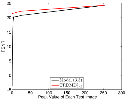
Figure 4: Performance comparison between the proposed diffusion model $\mathrm{TRDMD}_{5\times 5}^{5}$ and Model (3.3) for despeckling. The peak values of the test images are distributed between 0.5$\sim$255.

4.1 The Experimental Comparison Between the Diffusion Model (3.3) and $\mathrm{TRDMD}$

In this subsection, we conducted experiments based on the diffusion model (3.3), and compared its performance with the proposed model $\mathrm{TRDMD}$ in this study. For the sake of fairness, these methods are evaluated on synthesized images with speckle noise using 68 optical images, just as in the submitted paper. The test number of looks $L$ is set as 1. In order to perform a fast comparison, we employ the filter size $5\times 5$ and stage = 5 to setup the training models. Two cases as follows are considered for experimental analysis.

Case 1:

In this case, we take experiments directly on the 68 optical images whose minimum pixel value for each image is 1. The PSNR value obtained by the Model (3.3) is 24.30dB, just the same as $\mathrm{TRDMD}_{5\times 5}^{5}$, indicating that the Model (3.3) also works for images with pixel values bigger than 1.

Case 2:

In this case, we set the maximum value (peak value) of each of the 68 optical images to be 0.5$\sim$255 by dividing the ground-truth image $u_{gt}$ by a factor $n$, i.e., $u_{gt}=\frac{u_{gt}}{n}$. The obtained PSNR values along with the peak values are presented in Figure 4. From Figure 4 we can see that the gap between the two models decreases as the peak value increases. For lower peak values, the number of pixels that are smaller than 1 is bigger, leading to worse PSNR performance for Model (3.3). Especially, there is an inflection point around peak value 6. At this point, the number of pixels that are smaller than 1 becomes so large that the performance of Model (3.3) is degraded obviously.

In summary, in order to perform a stable training, we have to set $c=1$. However, the hard projection operation $u=\mathrm{max}(u,1)$ will obviously manipulate some of the pixels, because it will set those pixels that should be 0 or very close to 0 to be 1. If the number of those pixels is relatively small, it is not a problem. However, if there is a large number of dark areas in the target image, e.g., for the case of real SAR images, the projection $u=\mathrm{max}(u,1)$ will significant affect the despeckled results. As a consequence, the despeckling performance will degrade dramatically. In an extreme case, if we carry out a toy test on a constant image whose size is $256\times 256$ and pixel value is 0.5. The PSNR value obtained by the Model (3.3) is -0.01dB. However, the PSNR value obtained by $\mathrm{TRDMD}_{5\times 5}^{5}$ is 20.04dB, which is much higher than the Model (3.3).

Therefore, we mainly exploited the model $\mathrm{TRDMD}$ in this study.

4.2 Influence of The Number of Training Samples

In this subsection, we evaluate the despeckling performance of trained models using different amounts of training samples for $\mathrm{TRDMD}_{5\times 5}^{5}$.

The results are summarized in Fig. 5(a), from which one can see that too small training set will result in over-fitting which leads to inferior PSNR value. By observation, 400 images are typically enough to provide reliable performance.

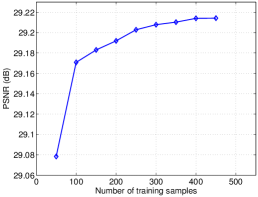
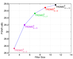
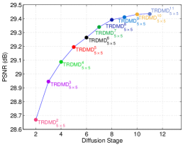
Figure 5: (a) Influence of the number of training examples. (b) Influence of the filter size. (c) Influence of the number of diffusion stages.

4.3 Influence of filter size

In this subsection, we investigate the influence of the filter size on the despeckling performance in Fig. 5(b). The diffusion stages are set as 5, and 400 images are used for training.

One can see that increasing the filter size keeps bringing improvement. However, the rate of increase in PSNR becomes relatively slower for larger filter size. Balancing the training time and the performance improvement, we choose the $\mathrm{TRDMD}_{7\times 7}^{T}$ model in our experiments.

(a) $Mountain$

(b) Noisy image. $L=1$

(c) $\Gamma$-Map (22.49/0.578/0.182)

(d) SRAD ( 23.47/0.728/0.300)

(e) DPAD (23.54/0.729/0.318)

(f) $\mathrm{TRDMD}_{7\times 7}^{10}$ (26.80/0.752/0.461)

Figure 6: Despeckling of $Mountain$ with $L=1$. The results are reported by PSNR/MSSIM/EC index. Best results are marked.

4.4 Influence of Diffusion Stages

In this study, any number of diffusion stages can be exploited in our model. But in practice, the trade-off between run time and accuracy should be considered. Therefore, we need to study the influence of the number of diffusion stages on the denoising performance. $\mathrm{TRDMD}_{5\times 5}^{T}$ and 400 images are used for training.

As shown in Fig. 5(c), the performance improvement becomes quite insignificant when the diffusion stages $\geq 10$. In order to save the training time, we choose $\mathrm{diffusion\;stage}=10$ in the following experiments as it provides the best trade-off between performance and computation time.

(a) $water$ $castle$

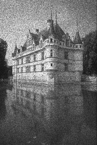
(b) Noisy image. $L=3$

(c) $\Gamma$-Map (23.27/0.687/0.420)

(d) SRAD (25.38/0.799/0.525)

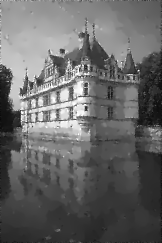
(e) DPAD (25.45/0.799/0.532)

(f) $\mathrm{TRDMD}_{7\times 7}^{10}$ (27.20/0.817/0.647)

Figure 7: Despeckling of $Tower$ with $L=3$. The results are reported by PSNR/MSSIM/EC index. Best results are marked.

4.5 Experimental Results

By analyzing the above three subsections, we decide to employ $\mathrm{TRDMD}_{7\times 7}^{10}$ model and 400 images for training. Note that, the diffusion model needs to be trained respectively for different number of looks.

4.5.1 Comparison with Traditional Anisotropic Diffusion Based Approaches

	$L$=1	$L$=3	$L$=5	$L$=8
	PSNR/MSSIM/EC	PSNR/MSSIM/EC	PSNR/MSSIM/EC	PSNR/MSSIM/EC
$\Gamma$-Map	21.02/0.513/0.238	23.46/0.651/0.394	24.70/0.708/0.469	25.97/0.757/0.540
SRAD	24.82/0.686/0.465	25.42/0.738/0.489	26.92/0.790/0.570	28.25/0.819/0.639
DPAD	24.78/0.681/0.473	25.48/0.735/0.499	27.00/0.789/0.577	28.29/0.818/0.643
$\mathrm{TRDMD}_{7\times 7}^{10}$	24.95/0.678/0.479	27.28/0.775/0.630	28.53/0.819/0.700	29.70/0.852/0.754

Table 1: Comparison of the performance of the test algorithms in terms of PSNR, MSSIM and EC. Best results are marked.

In this subsection, we compare the proposed despeckling model with the $\Gamma$-Map filter [36] and some related anisotropic diffusion approaches, e.g., speckle reducing anisotropic diffusion (SRAD) [53] and detail preserving anisotropic diffusion (DPAD) [3]. Moreover, to ensure that SRAD and DPAD achieve their best performance respectively, we set a time step $\Delta t=0.2$ and run 400-3000 iterations for different noise levels.

By observation on despeckling performances in Fig. 6 and Fig. 7, we can see that in comparison with the $\Gamma$-Map filter, the other three methods show superior performance on edge localization and detail preservation. However, the unnatural smoothness introduced after iterative processing makes SRAD and DPAD produce cartoon-like images, i.e., made up by textureless geometric patches. Therefore, SRAD and DPAD may be unsuitable for practical application, because fine details and textures that may be useful for analysis are destroyed. On the contrary, the proposed method produces more natural results in visual quality and preserves more detailed information.

Quantitative evaluation results are shown in Table 1. Overall speaking, DPAD gives slightly better results than SRAD in terms of evaluation indexes. Meanwhile, Table 1 show that the best indexes are provided by the proposed model, indicating that the proposed model is more powerful in structural and edge preservation.

4.5.2 Comparison with State-of-the-art Despeckling Approaches

In this subsection, we compare the proposed despeckling model with several state-of-the-art despeckling approaches, i.e., the nonlocal methods PPBit [18], SAR-BM3D [42], and our previous FoE-based despeckling work [12].

Examining the recovery images with $L=1$ in Fig. 8, we see that in comparison with PPBit and FoE, the proposed method and SAR-BM3D work better at capturing textures, details and small features. On the other hand, in comparison with SAR-BM3D, the proposed method recovers clearer edges and is relatively less disturbed by artifacts. As shown in Fig. 8(d)-Fig. 11(d) the despeckled results of SAR-BM3D are affected by the structured signal-like artifacts that appear in homogeneous areas of the image. This phenomenon is originated from the selection process in the BM3D denoising process. The selection process is easily influenced by the noise itself, especially in flat areas of the image, which can be dangerously self-referential.

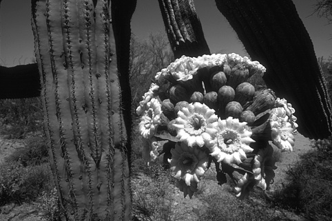
(a) $Flower$

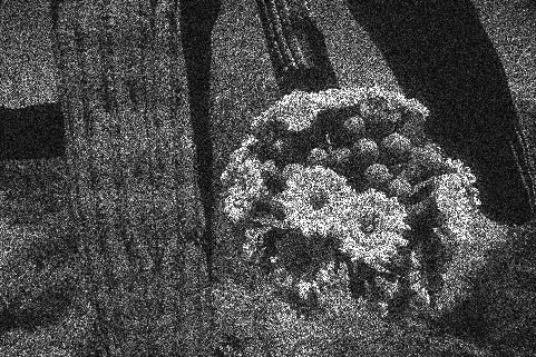
(b) Noisy image. $L=1$

(c) PPBit (23.22/0.595/0.278)

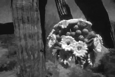
(d) SAR-BM3D (24.40/0.672/0.354)

(e) FoE (24.08/0.637/0.388)

(f) $\mathrm{TRDMD}_{7\times 7}^{10}$ (24.53/0.675/0.392)

Figure 8: Despeckling of $Flower$ with $L=1$. The results are reported by PSNR/MSSIM/EC index. Best results are marked.

(a) $Race$

(b) Noisy image. $L=5$

(c) PPBit (26.80/0.722/0.616)

(d) SAR-BM3D (28.06/0.769/0.714)

(e) FoE (27.94/0.755/0.745)

(f) $\mathrm{TRDMD}_{7\times 7}^{10}$ (28.36/0.772/0.751)

Figure 9: Despeckling of $Race$ with $L=5$. The results are reported by PSNR/MSSIM/EC index. Best results are marked.

(a) $Race$

(b) Noisy image. $L=5$

(c) PPBit

(d) SAR-BM3D

(e) FoE

(f) $\mathrm{TRDMD}_{7\times 7}^{10}$

Figure 10: The magnified despeckling results within the red rectangle in Fig. 9(a).

	$L$=1	$L$=3	$L$=5	$L$=8
	PSNR/MSSIM/EC	PSNR/MSSIM/EC	PSNR/MSSIM/EC	PSNR/MSSIM/EC
Noisy	12.95/0.223/0.148	17.42/0.378/0.255	19.59/0.460/0.322	21.61/0.535/0.393
PPBit	23.78/0.590/0.346	25.95/0.713/0.487	26.95/0.763/0.549	27.86/0.803/0.602
SAR-BM3D	24.85/0.676/0.455	27.12/0.776/0.605	28.27/0.818/0.669	29.35/0.852/0.723
FoE	24.65/0.669/0.493	27.07/0.763/0.637	28.32/0.812/0.698	29.54/0.848/0.753
$\mathrm{TRDMD}_{7\times 7}^{10}$	24.95/0.678/0.479	27.28/0.775/0.630	28.53/0.819/0.700	29.70/0.852/0.754

Table 2: Comparison of the performance of the test algorithms in terms of PSNR, MSSIM and EC. Best results are marked.

In Fig. 9-Fig. 10 are reported the recovered results for $L=5$. For better visual comparison, we also provide the magnified results within the red rectangles shown in Fig. 9. By observation, one can see that the performance of $\mathrm{TRDMD}_{7\times 7}^{10}$ is better than FoE and SAR-BM3D on detail preservation. In the visual quality, the typical structured artifacts encountered with the BM3D-based algorithm do not appear when the proposed method $\mathrm{TRDMD}_{7\times 7}^{10}$ is used. Moreover, our method works better in geometry-preserving than FoE, which can be visually perceived by comparison on (e) and (f) in Fig. 10. Actually, one can see that functional (2.9) is exactly the fields of experts (FoE) image prior regularized variational model for image restoration. However, in the $\mathrm{TRDMD}_{7\times 7}^{10}$ model, both the linear filters and influence functions are trained and optimized, which is the critical factor for the effectiveness of the proposed diffusion despeckling model. This critical factor of the optimized diffusion model is quite different from the FoE prior based variational model and traditional convolutional networks, where only linear filters are trained with fixed influence functions.

The recovery error in terms of PSNR (in dB) and MSSIM are summarized in Table 2. Comparing the indexes in Table 2, the overall performance of $\mathrm{TRDMD}_{7\times 7}^{10}$ in terms of PSNR/MSSIM is better than the other methods. This indicates that for most images our method is powerful in the recover quality and geometry feature preservation. Overall speaking, the proposed model and SAR-BM3D perform better than the other test methods in terms of texture and detail preservation, as illustrated in the MSSIM index. In addition, according to the EC index, the proposed model preserves more clearer edges in comparison with SAR-BM3D.

We also present the despeckling results for real SAR amplitude images in Fig. 11-Fig. 12. The test four SAR images are as follows: 1) single-look Radarsat-1 image of Vancouver (Canada) in Fig. 11, identified as $Vancouver$; 2) single-look SAR images identified as $Bayard$ and $Cheminot$ from Saint-Pol-sur-Mer (France), sensed in 1996 by RAMSES of ONERA, as shown in Fig. 11; and 3) six-look AirSAR cropland scene identified as $Cropland$, as shown in Fig. 12. By closely visual comparison, we can observe that $\mathrm{TRDMD}_{7\times 7}^{10}$ recovers clearer texture and sharper edges. Especially for the tiny features, $\mathrm{TRDMD}_{7\times 7}^{10}$ is able to catch but the other methods neglects them. Although these features are not quite obvious, the trained diffusion model still extracts them and exhibit these features apparently.

Table 3 lists the three without-reference indexes of the different algorithms on four real SAR images. Comparing the indexes in Table 3, one can see that no algorithm is predominant in the despeckling performance. However, overall speaking, the proposed model provides most preferable results in terms of the evaluation indexes. Overall speaking, the proposed model provides comparable or even better results than the test state-of-the-art methods, both in visual effects and the numerical indexes.

Image	Index	Ideal	PPBit	BM3D	FoE	$\mathrm{TRDMD}$
	RI$\_$M	1	0.862	0.873	0.913	0.900
$Vancouver$	RI$\_$V	0.273	0.198	0.179	0.195	0.179
	$C_{u}$	0.304	0.236	0.284	0.281	0.314
	RI$\_$M	1	0.861	0.850	1.020	0.859
$Bayard$	RI$\_$V	0.273	0.178	0.157	0.073	0.203
	$C_{u}$	0.770	0.744	0.736	0.838	0.750
	RI$\_$M	1	0.863	0.837	1.027	0.847
$Cheminot$	RI$\_$V	0.273	0.165	0.147	0.060	0.203
	$C_{u}$	0.844	0.848	0.808	0.932	0.829
	RI$\_$M	1	0.974	0.969	0.965	0.973
$Cropland$	RI$\_$V	0.046	0.037	0.038	0.028	0.048
	$C_{u}$	0.337	0.412	0.415	0.426	0.423

Table 3: Comparison of the performance of the test algorithms on real SAR images. Best results are marked. Note that in the table BM3D refers to SAR-BM3D method and $\mathrm{TRDMD}$ denotes $\mathrm{TRDMD}_{7\times 7}^{10}$.

4.5.3 Run Time

The proposed method merely contains convolution of linear filters with an image, which offers high computation efficiency and high levels of parallelism making it well suited for GPU implementation. More precisely, the proposed model can not only run fast on CPU especially when the 2-D convolution is efficiently realized by FFT, but also be implemented using GPU. Even without GPU, the proposed model is efficient enough.

In Table 4, we report the typical run time of our model for the images of two different dimensions for the case of $L=8$. It is worthy noting that the FoE-based method needs more iterations to converge if the noise level is higher. Therefore, for $L=1,3$ or 5, the consuming time of FoE-based method is more than $L=8$. We also present the run time of four competing algorithms for a comparison. Note that the method FANS [15] is the improved version of SAR-BM3D, at the expense of slight performance degradation. Meanwhile, the main body of SAR-BM3D, PPBit and FANS are all implemented in C language. All the methods are run in Matlab with single-threaded computation for CPU implementation.

Due to the structural simplicity of our model, it is well-suited to GPU parallel computation. We are able to implement our algorithm on GPU with ease. It turns out that the GPU implementation based on NVIDIA Geforce GTX 780Ti can accelerate the inference procedure significantly, as shown in Table 4. By comparison, we see that our $\mathrm{TRDMD}_{7\times 7}^{10}$ model is generally faster than the other methods, especially with GPU implementation. This is reasonable because the PPBit and SAR-BM3D are based nonlocal approach with high computation complexity. For FoE-based method, the required maximum number of iterations is 120 for $L=8$, 150 for $L=5$, 300 for $L=3$ and 600 for $L=1$. On the contrary, our $\mathrm{TRDMD}_{7\times 7}^{10}$ model needs only 10 iteration steps with similar amount of computations at each step in comparison with FoE.

	SAR-BM3D	FANS	PPBit	FoE ($L$=8)	$\mathrm{TRDMD}_{7\times 7}^{10}$
$256\times 256$	42.4	3.71	13.2	14.86(0.12)	3.05 (0.03)
$512\times 512$	169.1	14.40	48.9	59.43(0.37)	9.33 (0.09)

Table 4: Typical run time (in second) of the Despeckling methods for images with two different dimensions. The CPU computation time is evaluated on Intel CPU X5675, 3.07GHz. The highlighted number is the run time of GPU implementation based on NVIDIA Geforce GTX 780Ti.

(a) $Vancouver$. $L=1$

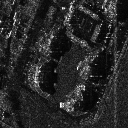
(b) $Bayard$. $L=1$

(c) $Cheminot$. $L=1$

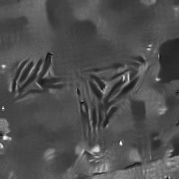
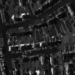
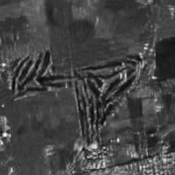
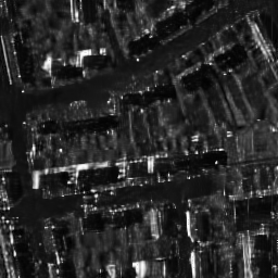
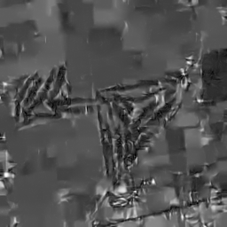
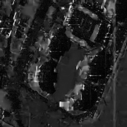
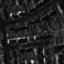
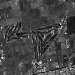
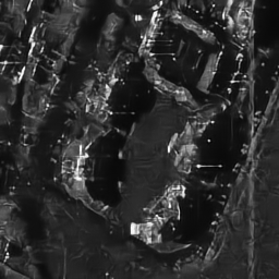
Figure 11: Despeckling of real SAR images with $L=1$. The employed methods are PPBit (the second row), SAR-BM3D (the third row), FoE (the fourth row) and the proposed $\mathrm{TRDMD}_{7\times 7}^{10}$ (the fifth row).

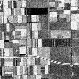
(a) $Cropland$. $L=6$

(b) PPBit

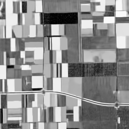
(c) SAR-BM3D

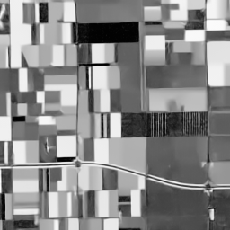
(d) FoE

(e) $\mathrm{TRDMD}_{7\times 7}^{10}$

Figure 12: Despeckling of $Cropland$ with $L=6$.

5 Conclusion

In this study we proposed a simple but effective despeckling approach with both high computational efficiency and comparable or even better results than state-of-the-art approaches. We achieve this goal by exploiting the newly-developed trainable nonlinear reaction diffusion model. The linear filters and influence functions in the model are simultaneously optimized by taking into account the speckle noise statistics.

The proposed model merely contains convolution of linear filters with an image, which offers high computation efficiency on CPU. Moreover, high levels of parallelism in the proposed model make it well suited for GPU implementation. Therefore, the proposed model is able to deal with massive-scale and huge amount of data. In comparison with several related anisotropic diffusion despeckling approaches with handcrafted filters and unique influence function, e.g., SRAD and DPAD, the proposed model provides a much enhanced performance in both visual effects and evaluation indexes. In comparison with the nonlocal-based PPBit and SAR-BM3D methods, the proposed model bears the properties of simple structure and high efficiency with strongly competitive despeckling performance.

Note that, the training data is our study is natural images. Hence, the despeckling performance on real SAR images could be enhanced if the remote sensing dataset is employed for training.

References

- [1] A. Achim, E. E. Kuruoğlu, and J. Zerubia. SAR image filtering based on the heavy-tailed rayleigh model. Image Processing, IEEE Transactions on, 15(9):2686–2693, 2006.
- [2] A. Achim, P. Tsakalides, and A. Bezerianos. SAR image denoising via bayesian wavelet shrinkage based on heavy-tailed modeling. Geoscience and Remote Sensing, IEEE Transactions on, 41(8):1773–1784, 2003.
- [3] S. Aja-Fernández and C. Alberola-López. On the estimation of the coefficient of variation for anisotropic diffusion speckle filtering. Image Processing, IEEE Transactions on, 15(9):2694–2701, 2006.
- [4] L. Alparone, S. Baronti, A. Garzelli, and F. Nencini. Landsat ETM+ and SAR image fusion based on generalized intensity modulation. Geoscience and Remote Sensing, IEEE Transactions on, 42(12):2832–2839, 2004.
- [5] F. Argenti, T. Bianchi, A. Lapini, and L. Alparone. Fast map despeckling based on Laplacian–Gaussian modeling of wavelet coefficients. Geoscience and Remote Sensing Letters, IEEE, 9(1):13–17, 2012.
- [6] F. Argenti, A. Lapini, T. Bianchi, and L. Alparone. A tutorial on speckle reduction in synthetic aperture radar images. IEEE GEOSCIENCE AND REMOTE SENSING MAGAZINE, 1(3):6–35, 2013.
- [7] G. Aubert and J.-F. Aujol. A variational approach to removing multiplicative noise. SIAM Journal of Applied Mathematics, 68(4):925–946, 2008.
- [8] T. Bianchi, F. Argenti, and L. Alparone. Segmentation-based map despeckling of SAR images in the undecimated wavelet domain. Geoscience and Remote Sensing, IEEE Transactions on, 46(9):2728–2742, 2008.
- [9] K. Bredies, K. Kunisch, and T. Pock. Total generalized variation. SIAM J. Imaging Sciences, 3(3):492–526, 2010.
- [10] A. Buades, B. Coll, and J.-M. Morel. A review of image denoising algorithms, with a new one. Multiscale Modeling & Simulation, 4(2):490–530, 2005.
- [11] L. Chen, X. Liu, X. Wang, and P. Zhu. Multiplicative noise removal via nonlocal similarity-based sparse representation. Journal of Mathematical Imaging and Vision, 54(2):199–215, 2016.
- [12] Y. Chen, W. Feng, R. Ranftl, H. Qiao, and T. Pock. A higher-order MRF based variational model for multiplicative noise reduction. Signal Processing Letters, IEEE, 21(11):1370–1374, 2014.
- [13] Y. Chen and T. Pock. Trainable Nonlinear Reaction Diffusion: A flexible framework for fast and effective image restoration. To appear in IEEE TPAMI, 2016.
- [14] Y. Chen, W. Yu, and T. Pock. On learning optimized reaction diffusion processes for effective image restoration. In Proc. IEEE Conference on Computer Vision and Pattern Recognition (CVPR), 2015.
- [15] D. Cozzolino, S. Parrilli, G. Scarpa, G. Poggi, and L. Verdoliva. Fast adaptive nonlocal SAR despeckling. IEEE Geosci. Remote Sensing Lett., 11(2):524–528, 2014.
- [16] I. Csiszár. Why least squares and maximum entropy? an axiomatic approach to inference for linear inverse problems. The annals of statistics, 19(4):2032–2066, 1991.
- [17] K. Dabov, A. Foi, V. Katkovnik, and K. Egiazarian. Image denoising by sparse 3-d transform-domain collaborative filtering. Image Processing, IEEE Transactions on, 16(8):2080–2095, 2007.
- [18] C.-A. Deledalle, L. Denis, and F. Tupin. Iterative weighted maximum likelihood denoising with probabilistic patch-based weights. Image Processing, IEEE Transactions on, 18(12):2661–2672, 2009.
- [19] C.-A. Deledalle, L. Denis, and F. Tupin. How to compare noisy patches? patch similarity beyond gaussian noise. International journal of computer vision, 99(1):86–102, 2012.
- [20] G. Di Martino, M. Poderico, G. Poggi, D. Riccio, and L. Verdoliva. Benchmarking framework for SAR despeckling. Geoscience and Remote Sensing, IEEE Transactions on, 52(3):1596–1615, 2014.
- [21] Y. Dong and T. Zeng. A convex variational model for restoring blurred images with multiplicative. SIAM J. Imaging Sciences, 6(3):1598–1625, 2013.
- [22] S. Durand, J. Fadili, and M. Nikolova. Multiplicative noise removal using l1 fidelity on frame coefficients. Journal of Mathematical Imaging and Vision, 36(3):201–226, 2010.
- [23] M. Elad and M. Aharon. Image denoising via sparse and redundant representations over learned dictionaries. Image Processing, IEEE Transactions on, 15(12):3736–3745, 2006.
- [24] P. Escande, P. Weiss, and W. Zhang. A variational model for multiplicative structured noise removal.
- [25] W. Feng, H. Lei, and Y. Gao. Speckle reduction via higher order total variation approach. Image Processing, IEEE Transactions on, 23(4):1831–1843, April 2014.
- [26] V. Frost, K. Shanmugan, and J. Holtzman. A model for radar images and its applications to adaptive digital filtering of multiplicative noise. IEEE Trans. Pattern Anal. Mach. Intell., 4(2):157–166, 1982.
- [27] J. W. Goodman. Statistical properties of laser speckle patterns. In Laser speckle and related phenomena, pages 9–75. Springer, 1975.
- [28] Y.-M. Huang, D.-Y. Lu, and T. Zeng. Two-step approach for the restoration of images corrupted by multiplicative noise. SIAM J. Scientific Computing, 35(6), 2013.
- [29] Y.-M. Huang, L. Moisan, M. K. Ng, and T. Zeng. Multiplicative noise removal via a learned dictionary. Image Processing, IEEE Transactions on, 21(11):4534–4543, 2012.
- [30] Z. Jin and X. Yang. A variational model to remove the multiplicative noise in ultrasound images. Journal of Mathematical Imaging and Vision, 39(1):62–74, 2011.
- [31] D. T. Kuan, A. Sawchuk, T. C. Strand, and P. Chavel. Adaptive restoration of images with speckle. Acoustics, Speech and Signal Processing, IEEE Transactions on, 35(3):373–383, 1987.
- [32] Y. LeCun, L. Bottou, Y. Bengio, and P. Haffner. Gradient-based learning applied to document recognition. Proceedings of the IEEE, 86(11):2278–2324, 1998.
- [33] J.-S. Lee. Digital image enhancement and noise filtering by use of local statistics. Pattern Analysis and Machine Intelligence, IEEE Transactions on, (2):165–168, 1980.
- [34] J.-S. Lee. Refined filtering of image noise using local statistics. Computer graphics and image processing, 15(4):380–389, 1981.
- [35] D. C. Liu and J. Nocedal. On the limited memory BFGS method for large scale optimization. Mathematical Programming, 45(1):503–528, 1989.
- [36] A. Lopes, E. Nezry, R. Touzi, and H. Laur. Maximum a posteriori speckle filtering and first order texture models in SAR images. In Geoscience and Remote Sensing Symposium, 1990, pages 2409–2412, 1990.
- [37] A. Lopes, E. Nezry, R. Touzi, and H. Laur. Structure detection and statistical adaptive speckle filtering in SAR images. International Journal of Remote Sensing, 14(9):1735–1758, 1993.
- [38] D. Martin, C. Fowlkes, D. Tal, and J. Malik. A database of human segmented natural images and its application to evaluating segmentation algorithms and measuring ecological statistics. In Proc. 8th Int’l Conf. Computer Vision, 2001.
- [39] Y. Nesterov. Introductory lectures on convex optimization, volume 87 of Applied Optimization. Kluwer Academic Publishers, Boston, MA, 2004. A basic course.
- [40] P. Ochs, Y. Chen, T. Brox, and T. Pock. iPiano: Inertial Proximal Algorithm for Nonconvex Optimization. SIAM J. Imaging Sciences, 7(2):1388–1419, 2014.
- [41] C. Oliver and S. Quegan. Understanding synthetic aperture radar images. SciTech Publishing, 2004.
- [42] S. Parrilli, M. Poderico, C. V. Angelino, and L. Verdoliva. A nonlocal SAR image denoising algorithm based on LLMMSE wavelet shrinkage. IEEE T. Geoscience and Remote Sensing, 50(2):606–616, 2012.
- [43] P. Perona and J. Malik. Scale-space and edge detection using anisotropic diffusion. Pattern Analysis and Machine Intelligence, IEEE Transactions on, 12(7):629–639, 1990.
- [44] J. Ranjani and S. J. Thiruvengadam. Dual-tree complex wavelet transform based SAR despeckling using interscale dependence. IEEE T. Geoscience and Remote Sensing, 48(6):2723–2731, 2010.
- [45] J. J. Ranjani and S. Thiruvengadam. Generalized SAR despeckling based on dtcwt exploiting interscale and intrascale dependences. Geoscience and Remote Sensing Letters, IEEE, 8(3):552–556, 2011.
- [46] S. Roth and M. J. Black. Fields of experts. International Journal of Computer Vision, 82(2):205–229, 2009.
- [47] F. Sattar, L. Floreby, G. Salomonsson, and B. Lovstrom. Image enhancement based on a nonlinear multiscale method. IEEE transactions on image processing, 6(6):888–895, 1997.
- [48] G. Steidl and T. Teuber. Removing multiplicative noise by douglas-rachford splitting methods. Journal of Mathematical Imaging and Vision, 36(2):168–184, 2010.
- [49] T. Teuber and A. Lang. A new similarity measure for nonlocal filtering in the presence of multiplicative noise. Computational Statistics & Data Analysis, 56(12):3821–3842, 2012.
- [50] T. Teuber and A. Lang. Nonlocal filters for removing multiplicative noise. Scale Space and Variational Methods in Computer Vision, 6667:50–61, 2012.
- [51] R. Touzi. A review of speckle filtering in the context of estimation theory. Geoscience and Remote Sensing, IEEE Transactions on, 40(11):2392–2404, 2002.
- [52] Z. Wang, A. C. Bovik, H. R. Sheikh, and E. P. Simoncelli. Image quality assessment: from error visibility to structural similarity. IEEE Trans. Image Process., 13(4):600–612, 2004.
- [53] Y. Yu and S. T. Acton. Speckle reducing anisotropic diffusion. Image Processing, IEEE Transactions on, 11(11):1260–1270, 2002.