Learning Non-local Image Diffusion for
Image Denoising
Abstract
Image diffusion plays a fundamental role for the task of image denoising. Recently proposed trainable nonlinear reaction diffusion (TNRD) model defines a simple but very effective framework for image denoising. However, as the TNRD model is a local model, the diffusion behavior of which is purely controlled by information of local patches, it is prone to create artifacts in the homogenous regions and over-smooth highly textured regions, especially in the case of strong noise levels. Meanwhile, it is widely known that the non-local self-similarity (NSS) prior stands as an effective image prior for image denoising, which has been widely exploited in many non-local methods. In this work, we are highly motivated to embed the NSS prior into the TNRD model to tackle its weaknesses. In order to preserve the expected property that end-to-end training is available, we exploit the NSS prior by a set of non-local filters, and derive our proposed trainable non-local reaction diffusion (TNLRD) model for image denoising. Together with the local filters and influence functions, the non-local filters are learned by employing loss-specific training. The experimental results show that the trained TNLRD model produces visually plausible recovered images with more textures and less artifacts, compared to its local versions. Moreover, the trained TNLRD model can achieve strongly competitive performance to recent state-of-the-art image denoising methods in terms of peak signal-to-noise ratio (PSNR) and structural similarity index (SSIM).
Index Terms:
image denoising, non-local self-similarity, reaction diffusion, loss-based training.I Introduction
Image denoising is one of the most fundamental processing in image processing and low-level computer vision. While it has been extensively studied, image denoising is still an active topic in image processing and computer vision. The goal of image denoising is to recover the clean image from its noisy observation , which is formulated as
| (1) |
where is the noise. In this paper, we assume is the additive Gaussian noise with zero mean and standard derivation .
During the past decades, a large number of new image denoising methods are continuously emerging. It is a difficult task to precisely categorize existing image denoising approaches. Generally speaking, most image denoising approaches can be categorized as spatial domain and transform domain based methods. Transform domain based methods first represent an image with certain orthonormal transform, such as wavelets [1], curvelets [2], contourlets [3], or bandelets [4], and then attempt to separate noise from the clean image by manipulating the coefficients according to the statistical characteristics of the clean image and noise.
Spatial domain based approaches attempt to utilize the correlations between adjacent pixels in an image. Depending on the way how to select those adjacent pixels, spatial domain based methods can be categorized as local and non-local methods. In local methods, only those adjacent pixels in a spatial neighborhood (probably with fixed shape and size) of the test pixel are investigated. Pixels in this small spatial range are named as an image patch, and the clean pixel value is estimated from this local patch. A large number of local algorithms have been proposed, including filtering based methods [5, 6, 7, 8], anisotropic diffusion based methods [9, 10, 11], variational methods with various image regularizers [12, 13, 14], and patch-based models via sparse representation [15, 16].


Local methods concentrate on the modeling of the patch itself. Nowadays, it is widely-known that another type of image prior is very effective for image denoising - nonlocal self-similarity (NSS) prior; that is, in natural images there are often many similar patches (i.e., nonlocal neighbors) to a given patch, which may be spatially far from it. Inspired by the seminal work of nonlocal means [17], the NSS prior has been widely exploited for image denoising in various framework, such as K-SVD algorithm with nonlocal modeling [18], nuclear norm minimization with nonlocal modeling [19], and Markov Random Fields with nonlocal modeling [20]. Usually, NSS prior based models can significantly improve their corresponding local versions. As a consequence, many state-of-the-art image denoising algorithms are built on the NSS prior, such as BM3D [21], LSSC [18], NCSR [22], and WNNM [19].
Usually, local methods cannot perform very well when the noise level is high, because the correlations between neighboring pixels have been corrupted by the severe noise. Therefore, it is generally believed that local models are not expected to compete with those nonlocal models, especially those state-of-the-art ones, in terms of restoration quality. However, with the help of techniques from machine learning, a few local models, such as opt-MRF [23], Cascade Shrinkage Fields (CSF) [24], and recently proposed Trainable Non-linear Reaction Diffusion (TNRD) [25], succeed achieving state-of-the-art denoising performance via appropriate modeling and supervised learning. It is noticeable that the TNRD model has demonstrated strongly competitive, even better performance against the best-reported nonlocal algorithm - WNNM, meanwhile with much higher computational efficiency.
As mentioned earlier, incorporating the NSS prior has succeeded to boost many image denoising algorithms. Therefore, we are highly motivated to introduce the NSS prior to the best-performing diffusion framework - TNRD to investigate whether it can also boost the TNRD model as usual.
I-A Our contributions
The goal of this paper is to embed the NSS prior into the TNRD model for the task of image denoising. To this end, we propose trainable non-local reaction diffusion (TNLRD) models. The contributions of this study are four-fold:
-
a)
We propose a compact matrix form to exploit the NSS prior, which can facilitate the subsequent formulations and derivations associated with the nonlocal modeling. In this work, the NSS prior is defined by a set of non-local filters. In a TNLRD model, the filter responses of similar patches generated by a local spatial filter are further filtered by its corresponding non-local filter.
-
b)
We construct the nonlocal diffusion process with fixed iterations, which is parameterized by iteration-varying local spatial filters, non-local filters and nonlinear influence functions. Deriving the gradients of the training loss function w.r.t those learning parameters is not trivial, due to the involved nonlocal structure. We provide detailed derivations, which greatly differ from the original TNRD model.
-
c)
The training phase is accomplished in a loss-specific manner, where a loss function measuring the difference between clean image and denoised image is utilized to optimize the model parameters. In this study, we investigate two different loss functions, namely PSNR-oriented quadratic loss and SSIM related loss.
-
d)
We conduct comprehensive experiments to demonstrate the denoising performance of the proposed TNLRD models. As illustrated in Section IV, the proposed TNLRD models outperform recent state-of-the-art methods in terms of PSNR and SSIM.
The following section are organized as follows. In Section 2, we give a brief review of the related works. In Section 3, we introduce the proposed TNLRD models and the training issue. In Section 4, we discuss the influence of the parameters in the proposed TNLRD models, then show the denoising comparison with the previous state-of-the-arts. Finally in Section 5, we draw the conclusion.
II Background and Related work
In this section, we first give a brief review of the TNRD model for image denoising, then introduce the NSS scheme.
II-A Trainable non-linear reaction diffusion model
Chen et. al [25] proposed a simple but effective framework for image restoration - TNRD, which is derived from the following energy functional
| (2) |
where the regularization term is a high-order MRFs - Fields of Experts (FoE) [26], defined by a set of linear filters and the penalty function . is the number of filters, denotes the 2D convolution operator. is the strength of data term.
With appropriate modeling of the regularization term, minimizing the energy functional (2) can lead to a denoised image. The steepest-descent procedure for minimizing the energy (2) reads as
| (3) |
where convolution kernel is obtained by rotating the kernel 180 degrees, is the influence function [27] or flux function [10], donates the time step.
The TNRD model truncates the gradient descent procedure (3) to iterations, and it then naturally leads to a multi-layer diffusion network with layers. This modification introduces additional flexibility to the diffusion process, as it becomes easier to train the influence function in this framework. Moreover, as it can be considered as a multi-layer network, we can exploit layer-varying parameters. Therefore, the TNRD model is given as the following diffusion network with layers.
| (4) |
Note that the parameters vary across the layers. is the input of the diffusion network. It is clear that each layer of (4) only involves a few image convolution operations, and therefore, it bears an interesting link to the convolutional networks (CN) employed for image restoration problems, such as [28].
The parameters of TNRD models in (4) is trained in a supervised manner. Given the pairs of noisy image and its ground-truth , the parameters are optimized by minimizing certain loss function , where is given by the inference procedure (4). The training procedure is formulated as
| (5) |
where . The training problem can be solved via gradient based algorithms, e.g., commonly used L-BFGS algorithm [29]. The gradients of the loss function with respect to are computed using the standard back-propagation technique widely used in the neural networks learning [30]. There are two training strategies to learn the diffusion processes: 1) the greedy training strategy to learn the diffusion process stage-by-stage; and 2) the joint training strategy to joint train all the stages simultaneously. Generally speaking, the joint training strategy performs better [25], and the greedy training strategy is often employed to provide a good initialization for the joint training. For simplicity, we just consider the joint training scheme to train a diffusion process by simultaneously tuning the parameters in all stages. The associated gradient is presented as follows,
| (6) |
II-B Non-local self-similarity scheme
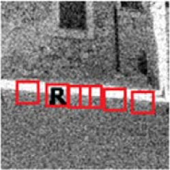
Based on the observation that one can always find a few similar patches to a reference patch in the same image, which might be significantly apart from the reference patch, an image prior named non-local self-similarity (NSS) was introduced in [17]. As described in Fig. 2, similar patches to a reference patch can be found in a significantly larger spatial range than the patch size. The non-local similar patches can be collected by using a k-nearest neighbor (k-NN) algorithm [20] or using a kernel function to map the patch distance to coefficients [31].
The NSS prior has proven highly effective for many image restoration problems, and it becomes greatly popular nowadays. A lot of state-of-the-art image restoration algorithms exploit this type of image prior, such as image denoising algorithms BM3D [21] and WNNM [19], image interpolation approaches NARM [31] and ANSM [32]. As a consequence, many local models also attempt to incorporate the NSS prior to boost the performance of the local versions, such as the LSSC method [18], which is a nonlocal extension of the K-SVD algorithm.
We want to especially emphasize the a NSS prior induced method - the NLR-MRF model proposed in [20], which extends the spatial range of the original FoE model [26], as it is highly related to our work. As described in [20], in the NLR-MRF model, several similar patches are firstly collected for each reference patch, and then the responses of these similar patches to a local filter are filtered by a cross-patch filter, generating more sparse responses compared with the local filter responses. With the extend spatial range, NLR-MRF models surpassed the original FoE models in both quality and quantity performance.
Our NSS prior extended TNRD model is also derived from a FoE prior based model. Compared with the TNLRD model to exploit in this paper, the NLR-MRF model is much more constrained in two aspects:
-
a)
It employs unchanged parameters for each iteration. However, our NLRD model makes use of iteration-varying parameters.
-
b)
Although the penalty functions in the NLR-MRF model are adjustable, they are functions of fixed shape (heavy-tailed functions with a single minimum at the point zero), such as Gaussian Scale Mixtures (GSM) or Student-t distribution. In the TNLRD model, the influence functions are parameterized via radial basis functions, which is able to generate functions of arbitrary shapes. As demonstrated in [25], those seemingly unconventional influence functions found by the training phase play a key role for the success of the TNRD model.
III Trainable non-local reaction diffusion models for image denoising
In this section, we first describe the non-local filter, then introduce the trainable non-local reaction diffusion for image denoising, coined as TNLRD. Finally we give the gradient derivation in the training issue.
III-A Compact matrix form to model the NSS prior
In this work, we make use of k-NN algorithm to collect a fixed number of similar patches. Similar patches are collected by block matching with mean squared error as patch similarity metrics in a large searching window. For the sake of computational efficiency, the size of searching window is set to be several times larger than that of the local spatial filters, as that in [21, 20, 19]. For each possible patch in an image of size (, and is represented as a column vector ), we collect similar patches (including the reference patch itself) via block matching. Therefore, after running block matching, we can obtain results summarized in Table I.
| index | 1 | 2 | 3 | ||||
In Table I, the numbers in each column indicate the indexes of the found similar patches to the corresponding reference patch. For example, in the column , the numbers indicate the indexes of similar patches to the reference patch , and the similar patches are sorted according to the distance to the reference patch, i.e., , where denotes an image patch centered at the point , and function is a distance measurement of two image patches.
Based on the results in Table I, we construct highly sparse matrices of size , namely, . only involves the information from the row of Table I. Each row of contains merely a non-zero number (exactly one), and its position is given by one of the indexes . For example, in the row of matrix , only the element at position is one, and the remaining elements are all zeros. It is easy to see that matrix is the identity matrix, i.e., . As shown later, the NSS prior can be easily embedded into the TNRD framework with the help of matrices .
In our work, we introduce a set of non-local filters to embed NSS priors into the TNRD model. A non-local filter is represented as a vector with elements, e.g., , whose value is assigned to the similar patch. In the TNLRD model, the filter response map generated by a spatial filter (i.e., ) is further filtered by a non-local filter , resulting a response map , then for the reference patch , its non-local filter response is given as
It turns out that the above formulation can be given in a more compact way, which reads as
where the matrix is defined by and the non-local filter , given as
| (7) |
In the following subsections, we will see that formulating the NSS prior in the way of (7) can significantly simplify the corresponding formulations, thus easier to understand and to follow, when compared to the formulations in [20]. In addition, the non-local filter in matrix form is also highly sparse, as each row of only has non-zero elements. As a result, can be efficiently stored via sparse matrix.
III-B Trainable non-local reaction diffusion
Following the formulation in the previous subsection to exploit the NSS prior, it is easy embed the NSS prior into the TNRD framework, and then we arrive at our proposed trainable non-local reaction diffusion.
In order to explain our proposed TNLRD model more clearly, we start from the following energy functional, which incorporates the NSS prior in a natural way
| (8) |
where is the latent image and the noisy image respectively, and is the number of pixels in image. The local convolution kernel in (2) is represented as its corresponding matrix form that is a highly sparse matrix, such that
is highly sparse matrix defined as in (7) to model the NSS prior, which is related to a non-local filter.
We follow the basic idea of TNRD that unfolds the gradient descent process as a multi-layer network model with layer-varying parameters, to derive the proposed TNLRD model. It is easy to firstly check that the gradient of the energy functional (8) with respect to is given as
| (9) |
where function is given as , matrix is the matrix form related to the linear kernel , which is obtained by rotating kernel 180 degrees 111 It should be noticed that the exact formulation for the first matrix in (9) should be . We make use of to simplify the model complexity. More details can be found in [25].
Therefore, our proposed non-local diffusion model is given as the following multi-layer network with layer-varying parameters
| (10) |
Note that the parameters in layer include local filters , non-local filters (i.e., matrix ), nonlinear functions and the trade-off parameter . The parameter set in layer is given as , where and .
According to the diffusion process (10), one can see that the TNRD model can be treated as a special case of the TNLRD models with , as the corresponding non-local diffusion model clearly degenerates to the local version given in (4), if we set .
In this work, we parameterize the local filters, non-local filters, nonlinear functions in the following way. Concerning the local filters, we follow the TNRD model, and exploit zero-mean filters of unit norm. This is accomplished by constructing the filter in the way of
| (11) |
where denotes the -norm, and is a filter bank. Therefore, it is clear that the filter is a linear combination of the basis filters in the filter bank. In order to achieve the property of zero-mean, the filter bank in this work is chosen as a modified DCT basis, which is obtained by removing the filter with constant entries from the complete DCT filters.
The non-local filters in the TNLRD models are vectors with unit length constraint. Therefore, we construct the non-local filter as
| (12) |
where is completely free of any constraint.
Following the work of TNRD, the nonlinear functions are parameterized via radial basis function (RBFs), i.e., function is represented as a weighted linear combination of a set of RBFs as follows,
| (13) |
where here is Gaussian RBFs with equidistant centers and unified scaling . The Gaussian radial basis is defined as
As described above, the proposed TNLRD model contains plenty of free parameters, which can be learned from training samples. In this work, we train the TNLRD model parameters in a loss-based learning manner. Given the pairs of degraded image and the ground-truth original image , the parameters are optimized by minimizing certain loss function , which is defined to measure the difference between the output , given by the inference procedure (10) and the desired output, i.e., the ground-truth .
In summary, the training procedure is formulated as
| (14) |
where the parameters . Note that we do not specify the form of the loss function in the training phase at present. The basic requirement for the loss function is that it should be differentiable. In our study, we consider two different loss functions for training, see Section IV-E.
III-C Gradients in the training phase for the TNLRD model
Usually, gradient-based algorithms are exploited to solve the corresponding optimization problem (14) in the training phase. Therefore, it is important to compute the gradients of cost function with respect to model parameters for TNLRD.
The gradient of loss function with respect to parameters in the layer , i.e., , is computed using back-propagation technique widely used in neural networks learning [30],
| (15) |
In the case of quadratic loss function, i.e.,
| (16) |
is directly derived from (16),
| (17) |
Now, we focus on the computation of the gradients , which are derived from the diffusion procedure (10).
III-C1 Computing
is computed as
| (19) |
Therefore, is given as
| (20) |
III-C2 Computing
Firstly, is computed as
| (21) |
where matrix is a diagonal matrix given as , . Matrix and are constructed from the images and of 2D form, respectively. For example, is constructed in the way that its rows are vectorized local patch extracted from image for each pixel, such that
The matrix is defined in the same way, and the image is given as . Matrix is a linear operator which inverts the vectorized kernel . In the case of a square kernel , it is equivalent to the Matlab command
As a consequence, is given as
| (22) |
III-C3 Computing
Therefore, is given as
| (25) |
III-C4 Computing
Firstly, and are defined as the vectorized form of matrix and respectively, holding that and . The relation between and reads as
where matrix is a rearrange matrix.
is computed from (10),
where , , , and . In the computation of , the following relations are useful, namely
and
where matrix and are highly sparse, given as
and
respectively.
Given that , is computed as
where is given as
where .
Combining these derivation, is computed as
| (26) |
As is computed from (7), is given as,
| (27) |
where . Then, we can obtain from (26) and (27), given as
| (28) |
As the non-local filter is parameterized by the coefficients as shown in (12), we need to additionally compute
| (29) |
The direct computation of is quite time-consuming and memory-inefficient. Benefit from the sparse matrix structure, matrix , and are not constructed explicitly. Therefore, the computation of is quite efficient. As mentioned above, matrix are highly sparse, each row of has precisely one non-zero value, and others are zeros. Therefore, the computation of can be interpreted as picking up values from indexed by . The computation of can be further simplified as
where , is the derivative of w.r.t. . Considering the sparse structure of , the indexing of is actually the indexing of and using in forms that described in Table I. The computational complexity of can be greatly reduced.
Implementation will be made publicly available after acceptance.
IV Experimental results
IV-A Training of TNLRD models
Concerning the model complexity 222While TNLRD models with more stages provide better denoising performance, they cost more time in both training and inference phase., the stages of inference is set to 5; the local filter size is set to and ; the number of non-local similar patches is set to 3, 5, 7, 9. The size of searching window is . The size of block matching is .
We trained the TNLRD models for Gaussian denoising problem with different standard deviation . We minimize (14) to learn the parameters of the TNLRD models with commonly used gradient-based L-BFGS [33]. The gradient of loss function with respect to parameters can be derived from (15) - (29). The training dataset of original and noisy image pairs is constructed over 400 images as [25] [24]. We cropped a region from each image, resulting in a total of 400 training images of size . In the training phase, computing the gradients of one stage for 400 images of size takes about 480 on a server with CPUs: Intel(R) Xeon E5-2650 @ 2.00GHz (eight cores). We run 200 L-BFGS iterations for optimization. Therefore, the total training time for model is . Implementation will be made publicly available after acceptance.
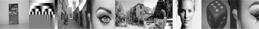
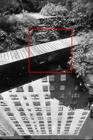
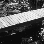
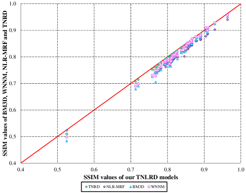
In order to perform a fair comparison to previous works, i.e., BM3D [21], WNNM [19], NLR-MRF [20] and TNRD [25], we used the 68 test images in [25], which are original introduced by [26] and are widely used in image denoising. We evaluated the denoising performance using PSNR as [25] and SSIM as [34]. SSIM provides a perceptually more plausible image error measure, which has been verified in psychophysical experiments. SSIM values range between 0 and 1, where 1 is a perfect restoration. We also test TNRD and our TNLRD models on a 9 image set which are collecting from web, as shown in Fig. 3. The codes of the comparison methods were downloaded from the authors’s homepage.
IV-B Influence of parameters initialization
The TNLRD models with different parameters configuration are denoted as, . The denotes the parameters initialization method, for initializing from the TNRD models, and for initializing from plain settings. In [20], the author trained NLR-MRF models starting from MRF models with local spatial clique, i.e., FoE models, using NSS setting. We followed the same training scheme as that in [20] for training NLR-MRF. We started from the local TNRD models by setting and , , and conducted a joint training for parameters of the steps inference (10), denoted as .
We also trained the parameters of TNLRD models via the greedy training from plain initialization, then jointly trained the steps inference (10), denoted as . Greedy training means a strategy that greedily trains a multi-layer diffusion network layer by layer. In the plain initialization training, we observed that TNLRD models with joint training surpass models obtained in greedy training by 0.55dB in average. Therefore, it is recommended that joint training should be conducted after greedy training.
We trained TNLRD models using both parameters initialization method, and got two models, namely and . We evaluated their denoising performance on the 68 test images. Models trained by and initialization achieve almost the same denoising performance, i.e., 29.01dB in average. This conclusion holds for our models with other model capacities. For the sake of training efficiency 333The plain initialization with greedy and joint training is more time consuming than the TNRD initialization which only conducts joint training., in the following experiments, we mainly discuss the models trained via TNRD initialization, which is coined as omitting the in .
IV-C Influence of number of non-local similar patches
In this subsection, we investigate the influence of different number of non-local similar patches for both and .
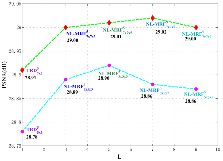
As described above, the TNRD model can be treated as a special case of the TNLRD model with . Therefore, in the training phase, the TNLRD model can be initialized from its local version. The denoising performance of the trained TNLRD models with different configurations are illustrated in Fig. 4. One can see that the performance of the trained models is improved when increases, and is degraded when continues to increase. A performance peak exists. for , it is ; for , it is . While a peak exists, the performance gap is within 0.05dB. For the sake of computational efficiency 444Larger will take more time for both training phase and test phase., in the rest of this section, we set . surpasses about 0.14dB. surpasses about 0.10dB.
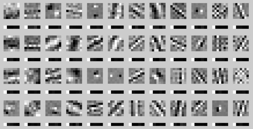
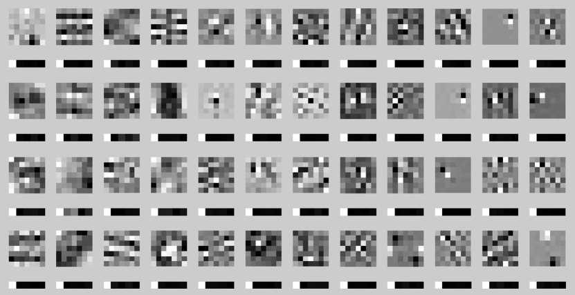
Fig. 5 shows the trained local and non-local filters of in the first and last inference stage, in the training of Gaussian denoising with . In most of the non-local filters, the first element is near 1, while the rest are near zero, for example ; while in some of the non-local filters, the first element is of the same scale with the rest, for example . The former non-local filters are related with simple local filters, for example the directional derivatives. The later non-local filters are related with complex local filters, hence all the local filter response of the similar patches are useful.
IV-D Influence of filter size
We also investigate the influence of filter size, as shown in Fig. 4. The increasing of the filter size from to brings an average 0.11dB improvement. In the evaluating of denoising performance, we prefer model as it provides better trade-off between performance and run time.
IV-E Influence of loss function
| Inference | Training | |||||
| L2 | SSIM | L2 | SSIM | L2 | SSIM | |
| PSNR | 31.50 | 0.8852 | 29.01 | 0.8201 | 26.06 | 0.7094 |
| SSIM | 31.31 | 0.8864 | 28.83 | 0.8219 | 25.80 | 0.7113 |
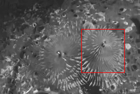
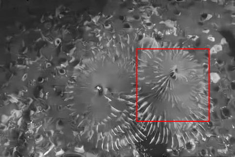
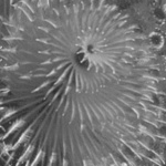
In [35, 36], the loss function for discriminative training is SSIM instead of L2 for image inpainting and denoising respectively. The trained models with SSIM loss function may provide visually more plausible results. Inspired by these works, we trained our TNLRD models using SSIM loss function as [34]. In the case of , the trained TNLRD models via SSIM loss achieves SSIM result of 0.8219, while the corresponding average PSNR is 28.83dB, as shown in Table II. The TNLRD models with the same capacity trained via the L2 loss, achieves a result of SSIM = 0.8201 and PSNR = 29.01dB. As shown in Fig. 6, the TNLRD models trained via SSIM loss offer sharper image than that trained via L2 loss. SSIM loss function benefits the TNLRD models to produce more visually plausible denoising results. From Table III, we note that our TNLRD models trained via SSIM loss achieve competitive performance with WNNM in terms of PSNR, and provide better recovered images in terms of SSIM. We also note that, compared with models trained via SSIM loss, models trained via L2 loss achieve competitive performance in terms of SSIM, and superior performance in terms of PSNR. Bearing these in mind, in the following comparison with other image denoising methods, we prefer the models trained with L2 loss.
IV-F Denoising


The above training experiments are conducted on Gaussian noise level . We also trained the proposed TNLRD models for the noise level and . After training the models, we evaluated them on the 68 test images used in [25]. We also tested the TNRD models and our TNLRD models on the 9 test image set.
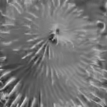
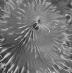
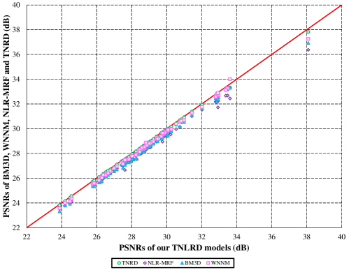
The denoising performance on the 68 test images is summarized in Table III and IV, compared with some recent state-of-the-art denoising algorithms. As illustrated in Table III and Fig. 12, the proposed TNLRD models outperform the TNRD models by almost 0.1dB, BM3D by 0.45dB, WNNM by 0.18dB and NLR-MRF by 0.53dB. In Fig. 6 (i-p), we can see that our TNLRD models recover more clear stems in the sea anemone than the TNRD models. While BM3D and WNNM tend to over-smooth texture regions, our TNLRD models produce sharper recovered image. In Fig. 7 (i-p), we can also see that clear and straight steel structures are recovered by our TNLRD models, while the TNRD models tends to offer the over-smooth results in the texture regions. The same phenomenon can be also found in the recovered image produced by BM3D and WNNM. Taking a close look at the recovered images produced by BM3D, WNNM and TNRD, one can see some artifacts in the plain regions.
We also compared our TNLRD model with these methods for cases of and , as shown in Table III. When the image is heavily degraded by the noise, i.e., is getting larger, the local methods, e.g., the TNRD model, can not collect enough information for inference, and may create artifacts and remove textures. On the contrary, the non-local methods collect more information, and tackle the artifacts and preserve textures. We show some denoising examples with in Fig. 8 and 9.
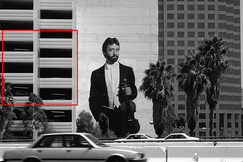
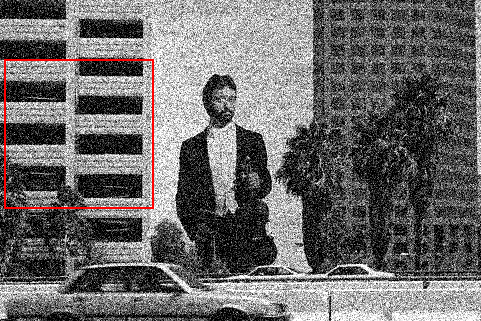


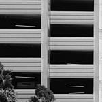
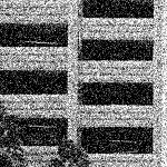

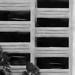


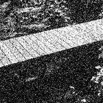
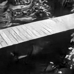

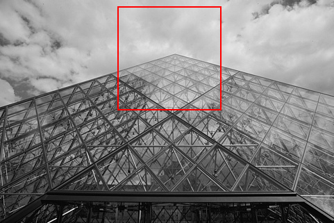
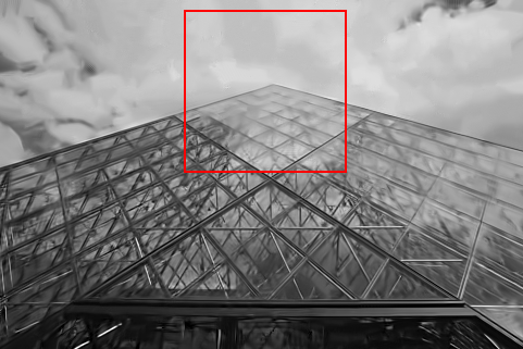
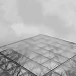
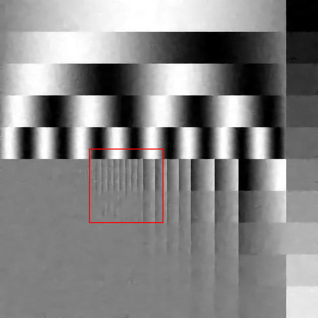
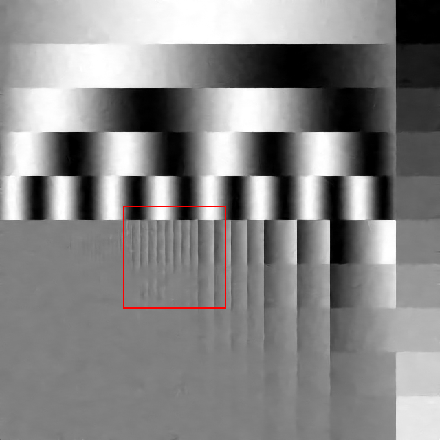
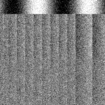
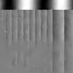
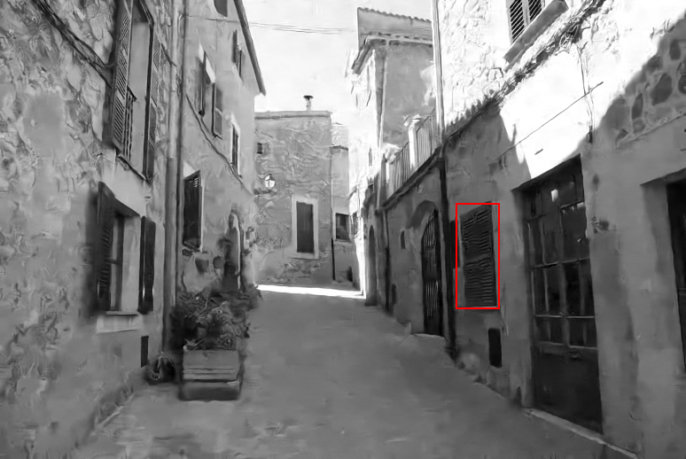
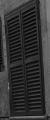
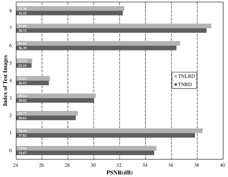
We also compare our TNLRD and TNRD on the 9 test images collected from web. In Fig. 10 (e-h), we can see that our TNLRD models recover the vertical lines more clear than the TNRD models. In Fig. 11 (e-h), we can see that our TNLRD models recover the window structures more precisely than the TNRD models. In Fig. 13, we can conclude that our TNLRD models surpass the TNRD models for each test image. The average PSNR produced by our TNLRD and TNRD models are 32.46dB and 32.24dB respectively.
From the detailed comparison with some state-of-the-art denoising methods, especially the newly proposed TNRD, we can conclude that our TNLRD models offer better quality and quantity performance in Gaussian denoising.


V Conclusion
In this paper, we propose trainable non-local reaction diffusion models for image denoising. We introduce the NSS prior as non-local filters to the TNRD models. We train the models parameters, i.e., local linear filters, non-local filters and non-linear influence functions, in a loss-based learning scheme. From the comparison with the state-of-the-art image denoising methods, we concluded that our TNLRD models achieve superior image denoising performance in terms of both PSNR and SSIM. Our TNLRD models also provide visually plausible denoised image with less artifacts and more textures.
References
- [1] E. P. Simoncelli and E. H. Adelson, “Noise removal via bayesian wavelet coring,” in Image Processing, 1996. Proceedings., International Conference on, vol. 1. IEEE, 1996, pp. 379–382.
- [2] J.-L. Starck, E. J. Candès, and D. L. Donoho, “The curvelet transform for image denoising,” IEEE Transactions on image processing, vol. 11, no. 6, pp. 670–684, 2002.
- [3] M. N. Do and M. Vetterli, “The contourlet transform: an efficient directional multiresolution image representation,” IEEE Transactions on image processing, vol. 14, no. 12, pp. 2091–2106, 2005.
- [4] E. Le Pennec and S. Mallat, “Sparse geometric image representations with bandelets,” IEEE transactions on image processing, vol. 14, no. 4, pp. 423–438, 2005.
- [5] C. Tomasi and R. Manduchi, “Bilateral filtering for gray and color images,” in Computer Vision, 1998. Sixth International Conference on. IEEE, 1998, pp. 839–846.
- [6] M. Elad, “On the origin of the bilateral filter and ways to improve it,” IEEE Transactions on image processing, vol. 11, no. 10, pp. 1141–1151, 2002.
- [7] H. Takeda, S. Farsiu, and P. Milanfar, “Kernel regression for image processing and reconstruction,” IEEE Transactions on image processing, vol. 16, no. 2, pp. 349–366, 2007.
- [8] S. Haykin and B. Widrow, Least-mean-square adaptive filters. John Wiley & Sons, 2003, vol. 31.
- [9] P. Perona and J. Malik, “Scale-space and edge detection using anisotropic diffusion,” IEEE Transactions on pattern analysis and machine intelligence, vol. 12, no. 7, pp. 629–639, 1990.
- [10] J. Weickert, Anisotropic diffusion in image processing. Teubner Stuttgart, 1998, vol. 1.
- [11] G. Gilboa, N. Sochen, and Y. Y. Zeevi, “Forward-and-backward diffusion processes for adaptive image enhancement and denoising,” IEEE transactions on image processing, vol. 11, no. 7, pp. 689–703, 2002.
- [12] L. I. Rudin, S. Osher, and E. Fatemi, “Nonlinear total variation based noise removal algorithms,” Physica D: Nonlinear Phenomena, vol. 60, no. 1, pp. 259–268, 1992.
- [13] T. Chan, A. Marquina, and P. Mulet, “High-order total variation-based image restoration,” SIAM Journal on Scientific Computing, vol. 22, no. 2, pp. 503–516, 2000.
- [14] S. Roth and M. J. Black, “Fields of experts: A framework for learning image priors,” in Proceedings of the IEEE Conference on Computer Vision and Pattern Recognition, vol. 2, 2005, pp. 860–867.
- [15] M. Elad and M. Aharon, “Image denoising via sparse and redundant representations over learned dictionaries,” IEEE Transactions on Image processing, vol. 15, no. 12, pp. 3736–3745, 2006.
- [16] M. Aharon, M. Elad, and A. Bruckstein, “K-svd: An algorithm for designing overcomplete dictionaries for sparse representation,” IEEE TRANSACTIONS ON SIGNAL PROCESSING, vol. 54, no. 11, p. 4311, 2006.
- [17] A. Buades, B. Coll, and J.-M. Morel, “A non-local algorithm for image denoising,” in Proceedings of the IEEE Conference on Computer Vision and Pattern Recognition, vol. 2, 2005, pp. 60–65.
- [18] J. Mairal, F. Bach, J. Ponce, G. Sapiro, and A. Zisserman, “Non-local sparse models for image restoration,” in Computer Vision, 2009 IEEE 12th International Conference on. IEEE, 2009, pp. 2272–2279.
- [19] S. Gu, L. Zhang, W. Zuo, and X. Feng, “Weighted nuclear norm minimization with application to image denoising,” in Proceedings of the IEEE Conference on Computer Vision and Pattern Recognition, 2014, pp. 2862–2869.
- [20] J. Sun and M. F. Tappen, “Learning non-local range markov random field for image restoration,” in Proceedings of the IEEE Conference on Computer Vision and Pattern Recognition, 2011, pp. 2745–2752.
- [21] K. Dabov, A. Foi, V. Katkovnik, and K. Egiazarian, “Image denoising by sparse 3-d transform-domain collaborative filtering,” Image Processing, IEEE Transactions on, vol. 16, no. 8, pp. 2080–2095, 2007.
- [22] W. Dong, L. Zhang, and G. Shi, “Centralized sparse representation for image restoration,” in 2011 International Conference on Computer Vision. IEEE, 2011, pp. 1259–1266.
- [23] Y. Chen, R. Ranftl, and T. Pock, “Insights into analysis operator learning: From patch-based sparse models to higher order mrfs,” IEEE Transactions on Image Processing, vol. 23, no. 3, pp. 1060–1072, 2014.
- [24] U. Schmidt and S. Roth, “Shrinkage fields for effective image restoration,” in Proceedings of the IEEE Conference on Computer Vision and Pattern Recognition, 2014, pp. 2774–2781.
- [25] Y. Chen, W. Yu, and T. Pock, “On learning optimized reaction diffusion processes for effective image restoration,” in Proceedings of the IEEE Conference on Computer Vision and Pattern Recognition, 2015, pp. 5261–5269.
- [26] S. Roth and M. J. Black, “Fields of experts,” International Journal of Computer Vision, vol. 82, no. 2, pp. 205–229, 2009.
- [27] M. Black, G. Sapiro, D. Marimont, and D. Heeger, “Robust anisotropic diffusion and sharpening of scalar and vector images,” in Image Processing, 1997. Proceedings., International Conference on, vol. 1. IEEE, 1997, pp. 263–266.
- [28] V. Jain and S. Seung, “Natural image denoising with convolutional networks,” in Advances in Neural Information Processing Systems, 2009, pp. 769–776.
- [29] D. C. Liu and J. Nocedal, “On the limited memory BFGS method for large scale optimization,” Mathematical Programming, vol. 45, no. 1, pp. 503–528, 1989.
- [30] Y. LeCun, L. Bottou, Y. Bengio, and P. Haffner, “Gradient-based learning applied to document recognition,” Proceedings of the IEEE, vol. 86, no. 11, pp. 2278–2324, 1998.
- [31] W. Dong, L. Zhang, R. Lukac, and G. Shi, “Sparse representation based image interpolation with nonlocal autoregressive modeling,” IEEE Trans. Image Processing, vol. 22, no. 4, pp. 1382–1394, 2013.
- [32] Y. Romano, M. Protter, and M. Elad, “Single image interpolation via adaptive nonlocal sparsity-based modeling,” IEEE Trans. Image Processing, vol. 23, no. 7, pp. 3085–3098, 2014.
- [33] D. C. Liu and J. Nocedal, “On the limited memory bfgs method for large scale optimization,” Mathematical programming, vol. 45, no. 1-3, pp. 503–528, 1989.
- [34] Z. Wang, A. C. Bovik, H. R. Sheikh, and E. P. Simoncelli, “Image quality assessment: From error visibility to structural similarity,” IEEE Trans. Image Processing, vol. 13, no. 4, pp. 600–612, 2004.
- [35] W. Yu, S. Heber, and T. Pock, “Learning reaction-diffusion models for image inpainting,” in GCPR, vol. 9358. Springer, 2015, pp. 356–367.
- [36] H. Zhao, O. Gallo, I. Frosio, and J. Kautz, “Is l2 a good loss function for neural networks for image processing?” arXiv preprint arXiv:1511.08861, 2015.