PairClone: A Bayesian Subclone Caller Based on Mutation Pairs

Abstract

Tumor cell populations can be thought of as being composed of homogeneous cell subpopulations, with each subpopulation being characterized by overlapping sets of single nucleotide variants (SNVs). Such subpopulations are known as subclones and are an important target for precision medicine. Reconstructing such subclones from next-generation sequencing (NGS) data is one of the major challenges in precision medicine. We present PairClone as a new tool to implement this reconstruction. The main idea of PairClone is to model short reads mapped to pairs of proximal SNVs. In contrast, most existing methods use only marginal reads for unpaired SNVs. Using Bayesian nonparametric models, we estimate posterior probabilities of the number, genotypes and population frequencies of subclones in one or more tumor sample. We use the categorical Indian buffet process (cIBP) as a prior probability model for subclones that are represented as vectors of categorical matrices that record the corresponding sets of mutation pairs. Performance of PairClone is assessed using simulated and real datasets. An open source software package can be obtained at http://www.compgenome.org/pairclone.

Keywords: Categorical Indian buffet process; Latent feature model; Local haplotype; Next-generation sequencing; Random categorical matrices; Subclone; Tumor heterogeneity.

1 Introduction

We explain intra-tumor heterogeneity by representing tumor cell populations as a mixture of subclones. We reconstruct unobserved subclones by utilizing information from pairs of proximal mutations that are obtained from next-generation sequencing (NGS) data. We exploit the fact that some short reads in NGS data cover pairs of phased mutations that reside on two sufficiently proximal loci. Therefore haplotypes of the mutation pairs can be observed and used for subclonal inference.

We develop a suitable sampling model that represents the paired nature of the data, and construct a nonparametric Bayesian feature allocation model as a prior for the hypothetical subclones. Both models together allow us to develop a fully probabilistic description of the composition of the tumor as a mixture of homogeneous underlying subclones, including the genotypes and number of such subclones.

1.1 Background

NGS technology (Mardis, 2008) has enabled researchers to develop bioinformatics tools that are being used to understand the landscape of tumors within and across different samples. An important related task is to reconstruct cellular subpopulations in one or more tumor samples, known as subclones. Mixtures of such subclones with varying population frequencies across spatial locations in the same tumor, across tumors from different time points, or across tumors from the primary and metastatic sites can provide information about the mechanisms of tumor evolution and metastasis. Heterogeneity of cell populations is seen, for example, in varying frequencies of distinct somatic mutations. The hypothetical tumor subclones are homogeneous. That is, a subclone is characterized by unique genomic variants in its genome  (Marjanovic et al., 2013; Almendro et al., 2013; Polyak, 2011; Stingl and Caldas, 2007; Shackleton et al., 2009; Dexter et al., 1978). Such subclones arise as the result of cellular evolution, which can be described by a phylogenetic tree that records how a sequence of somatic mutations gives rise to different cell subpopulations. Figure 1(a) provides a stylized and simple illustration in which a homogeneous sample with one original normal clone evolves into a heterogeneous sample with three subclones. Subclone 1 is the original parent cell population, and subclones 2 and 3 are descendant subclones of subclone 1, each possessing somatic mutations marked by the red letters. Each subclone possesses two homologous chromosomes (in black and green), and each chromosome in Figure 1(a) is marked by a triplet of letters representing the nucleotide on the three genomic loci. Together, the three subclones include four different haplotypes, (A, G, C), (A, G, T), (C, G, C), and (A, A, T), at these three genomic loci. In addition, each subclone has a different population frequency shown as the percentage values in Figure 1(a).

We use NGS data to infer such tumor heterogeneity. In an NGS experiment, DNA fragments are first produced by extracting the DNA molecules from the cells in a tumor sample. The fragments are then sequenced using short reads. For the three subclones in Figure 1(a), there are four aforementioned haplotypes at the three loci. Consequently, short reads that cover some of these three loci may manifest different alleles. For example, if a large number of reads cover the first two loci, we might observe (A, G), (C, G), (A, T) and (C, T), four alleles for the mutation pair. Observing four alleles is direct evidence supporting the presence of subclones (Sengupta et al., 2015). This is because, in the absence of copy number variations there can be only two haploid genomes at any loci for a homogeneous human sample. Therefore, one can use mutation pairs in copy neutral regions to develop statistical inference on the presence and frequency of subclones. This is the goal of our paper.

Almost all mutation-based subclone-calling methods in the literature use only single nucleotide variants (SNVs) (Oesper et al., 2013; Strino et al., 2013; Jiao et al., 2014; Miller et al., 2014; Roth et al., 2014; Zare et al., 2014; Deshwar et al., 2015; Sengupta et al., 2015; Lee et al., 2015, 2016). Instead of examining mutation pairs, SNV-based methods use marginal counts for each recorded locus only. Consider, for example, the first locus in Figure 1(a). At this locus, the reference genome has an “A” nucleotide while subclones 2 and 3 have a “C” nucleotide. In the entire sample, the “C” nucleotide is roughly present in 17.5% of the DNA molecules based on the population frequencies illustrated in Figure 1(a). The percentage of a mutated allele is called variant allele fraction (VAF). If a sample is homogeneous and assuming no copy number variations at the locus, the population frequency for the “C” nucleotide should be close to 0, 50%, or 100%, depending on the heterozygosity of the locus. Therefore, if the population frequency of “C” deviates from 0%, 50%, or 100%, the sample is likely to be heterogeneous. Based on this argument, SNV-based subclone callers search for SNVs with VAFs that are different from these frequencies (0, 50%, 100%), which are evidence for the presence of different (homogeneous) subpopulations. In the event of copy number variations, a similar but slightly more sophisticated reasoning can be applied, see for example, Lee et al. (2016).

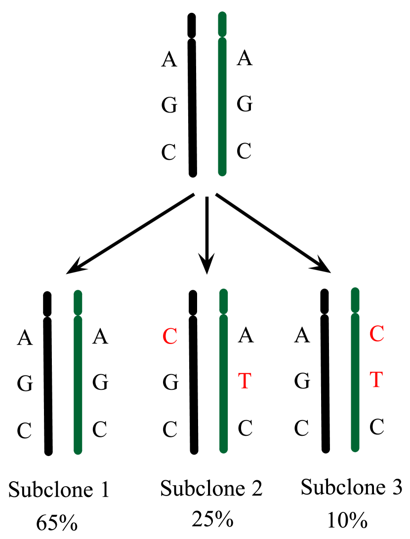
(a) Tumor evolution

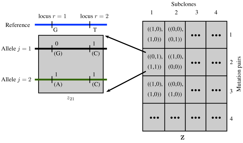
(b) Subclone structure matrix $\bm{Z}$

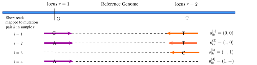
(c) Paired-end reads data

Figure 1: (a) Illustration of tumor evolution, emergence of subclones and their population frequencies. (b) Illustration of the subclone structure matrix $\bm{Z}$. Right panel: A subclone is represented by one column of $\bm{Z}$. Each element of a column represents the subclonal genotypes for a mutation pair. For example, the genotypes for mutation pair 2 in subclone 1 is ((0, 1), (1, 1)), which is shown in detail on the left panel. Left panel: The reference genome for mutation pair $2$ is (G, T) and the corresponding genotype of subclone $1$ is ((G, C), (A, C)), which gives rise to $\bm{z}_{21}=((0,1),(1,1))$. (c) Illustration of paired-end reads data for a mutation pair. Shown are four short reads mapped to mutation pair $k$ in sample $t$. Some reads are mapped to both loci of the mutation pair, and others are mapped to only one of the two loci. The two ends of the same read are marked with opposing arrows in purple and orange.

1.2 Using mutation pairs

NGS data usually contain substantially fewer mutation pairs than marginal SNVs. However, this does not weaken the power of using mutation pairs as mutation pairs naturally carry important phasing information that improves the accuracy of subclone reconstruction. For example, imagine a tumor sample that is a mixture of subclones 2 and 3 in Figure 1(a). Suppose a sufficient amount of short reads cover the first two loci, we should observe relatively large reads counts for four alleles (C, G), (A, T), (C, T) and (A, G). One can then reliably infer that there are heterogeneous cell subpopulations in the tumor sample. In contrast, if we ignore the phasing information and only consider the (marginal) VAFs for each SNV, then the observed VAFs for both SNVs are 50%, which could be heterogeneous mutations from a single cell population. See Simulation 1 for an illustration. In summary, we leverage the power of using mutation pairs over marginal SNVs by incorporating partial phasing information in our model. Besides the simulation study we will later also empirically confirm these considerations in actual data analysis.

The relative advantage of using mutation pairs over marginal SNV’s can be also be understood as a special case of a more general theme. In biomedical data it is often important to avoid overinterpretation of noisy data and to distill a relatively weak signal. A typical example is the probability of expression (POE) model of Parmigiani et al. (2002). Similarly, the modeling of mutation pairs is a way to extract the pertinent information from the massive noisy data. Due to noise and artifact in NGS data, such as base-calling or mapping error, many called SNVs might record unusual population frequencies, for reasons unrelated to the presence of subclones (Li, 2014). Direct modeling of all marginal read counts one ends up with noise swamping the desired signal (Nik-Zainal et al., 2012; Jiao et al., 2014). See our analysis of a real data set in Section 6 for an example. To mitigate this challenge, most methods use clustering of the VAFs, including, for example, Roth et al. (2014). One would then use the resulting cluster centers to infer subclones, which is one way of extracting more concise information. In addition, the vast majority of the methods in the literature show that even though a tumor sample could possess thousands to millions of SNVs, the number of inferred subclones usually is in the low single digit, no more than 10. To this end, we propose instead an alternative approach to extract useful information by modeling (fewer) mutation pairs, as mutation pairs contain more information and are of higher quality. We show in our numerical examples later that with a few dozens of these mutation pairs, the inference on the subclones is strikingly similar to cluster-based subclone callers using much more SNVs.

Finally, using mutation pairs does not exclude the possibility of making use of marginal SNVs. In Section 5.1, we show it is straightforward to jointly model mutation pairs and SNVs. Other biological complexities, such as tumor purity and copy number variations, can also be incorporated in our model. See Sections 5.2 and 5.3 for more details.

1.3 Representation of subclones

We construct a $K\times C$ categorical valued matrix $\bm{Z}$ (Figure 1(b)) to represent the subclone structure. Rows of $\bm{Z}$ are indexed by $k$ and represent mutation pairs, and a column of $\bm{Z}$, denoted by $\bm{z}_{c}=(\bm{z}_{1c},\cdots,\bm{z}_{Kc})$, records the phased mutation pairs on the two homologous chromosomes of subclone $c$, $c=1,\ldots,C$. As in Figure 1(b), let $j=1,2$ index the two homologous chromosomes, $r=1,2$ index the two mutation loci, $\bm{z}_{kc}=(\bm{z}_{kcj},j=1,2)$ be the genotype consisting of two alleles for mutation pair $k$ in subclone $c$, and $\bm{z}_{kcj}=(z_{kcjr},r=1,2)$ denote the allele of the $j$-th homologous chromosome. Therefore, each entry $\bm{z}_{kc}$ of the matrix $\bm{Z}$ is a $2\times 2$ binary submatrix itself. For example, in Figure 1(b) the entry $z_{21}$ is a pair of 2-dimension binary row vectors, $(0,1)$ and $(1,1)$, representing the genotypes for both alleles at mutation pair $k=2$ of subclone $c=1$; each vector indicates the allele for the mutation pair on a homologous chromosome. The first vector $(0,1)$ indicates that locus $r=1$ harbors no mutation (0) and locus $r=2$ harbors a mutation (1). Similarly, the second vector $(1,1)$ marks two mutations on both loci.

In summary, each entry of $\bm{Z}$,

$$\bm{z}_{kc}=\left(\bm{z}_{kc1},\bm{z}_{kc2}\right)=\left((z_{kc11},z_{kc12}),(z_{kc21},z_{kc22})\right)$$

is a $2\times 2$ matrix (with the two row vectors horizontally displayed for convenience). Each $z_{kcjr}$ is a binary indicator and $z_{kcjr}=1$ (or $0$) indicates a mutation (or reference). Thus, $\bm{z}_{kc}$ can take $Q=16$ possible values. That is, $\bm{z}_{kc}\in\{\bm{z}^{(1)},\ldots,\bm{z}^{(16)}\}=$ $\{(00,00),$ $(00,01),$ $\ldots,$ $(11,11)\}$, where we write $00$ short for $(0,0)$ etc., and $z^{(1)}=(00,00)$ refers to the genotype on the reference genome. Formally, $\bm{z}_{kc}$ is a $2\times 2$ binary matrix, and $\bm{Z}$ is a matrix of such binary matrices. Moreover, we can collapse some $\bm{z}^{(q)}$ values as we do not have phasing across mutation pairs. For example, $\bm{z}_{kc}=(01,10)$ and $\bm{z}_{kc}=(10,01)$, etc. have mirrored rows and are indistinguishable in defining a subclone (a column of $\bm{Z}$). (More details in Section 2.2). Typically distinct mutation pairs are distant from each other, and in NGS data they are almost never phased. Therefore, we can reduce the number of possible outcomes of $z_{kc}$ to $Q=10$, due to the mirrored outcomes. We list them below for later reference: $z^{(1)}=(00,00),z^{(2)}=(00,01),z^{(3)}=(00,10),z^{(4)}=(00,11),z^{(5)}=(01,01),z^{(6)}=(01,10),z^{(7)}=(01,11),z^{(8)}=(10,10),z^{(9)}=(10,11)$ and $z^{(10)}=(11,11)$. In summary, the entire matrix $\bm{Z}$ fully specifies the genomes of each subclone at all the mutation pairs.

Suppose $T$ tumor samples are available from the same patient, obtained either at different time points (such as initial diagnosis and relapses), at the same time but from different spatial locations within the same tumor, or from tumors at different metastatic sites. We assume those $T$ samples share the same subclones, while the subclonal population frequencies may vary across samples. For clinical decisions it can be important to know the population frequencies of the subclones. To facilitate such inference, we introduce a $T\times(C+1)$ matrix $\bm{w}$ to represent the population frequencies of subclones. The element $w_{tc}$ refers to the proportion of subclone $c$ in sample $t$, where $0<w_{tc}<1$ for all $t$ and $c$, and $\sum_{c=0}^{C}w_{tc}=1$. A background subclone, which has no biological meaning and is indexed by $c=0$, is included to account for artifacts and experimental noise. We will discuss more about this later.

The remainder of this article is organized as follows. In Sections 2 and 3, we propose a Bayesian feature allocation model and the corresponding posterior inference scheme to estimate the latent subclone structure. In Section 4, we evaluate the model with three simulation studies. Section 5 extends the models to accommodate other biological complexities and present additional simulation results. Section 6 reports the analysis results for a lung cancer patient with multiple tumor biopsies. We conclude with a final discussion in Section 7.

2 The PairClone Model

2.1 Sampling Model

Suppose paired-end short reads data are obtained by deep DNA sequencing of multiple tumor samples. In such data, a short read is obtained by sequencing two ends of the same DNA fragment. Usually a DNA fragment is much longer than a short read, and the two ends do not overlap and must be mapped separately. However, since the paired-end reads are from the same DNA fragment, they are naturally phased and can be used for inference of alleles and subclones. We use LocHap (Sengupta et al., 2015) to find pairs of mutations that are no more than a fixed number, say 500, base pairs apart. Such mutation pairs can be mapped by paired-end reads, making them eligible for PairClone analysis. See Figure 1(c) for an example. For each mutation pair, a number of short reads are mapped to at least one of the two loci. Denote the two sequences on short read $i$ mapped to mutation pair $k$ in tissue sample $t$ by $\bm{s}_{tk}^{(i)}=\left(s_{tkr}^{(i)},r=1,2\right)=\left(s_{tk1}^{(i)},s_{tk2}^{(i)}\right)$, where $r=1,2$ index the two loci, $s_{tkr}^{(i)}=0\mbox{ or }1$ indicates that the short read sequence is a reference or mutation. Theoretically, each $s_{tkr}^{(i)}$ can take four values, A, C, G, T, the four nucleotide sequences. However, at a single locus, the probability of observing more than two sequences across short reads is negligible since it would require the same locus to be mutated twice throughout the life span of the person or tumor, which is unlikely. We therefore code $s_{tkr}^{(i)}$ as a binary value. Also, sometimes a short read may cover only one of the two loci in a pair, and we use $s_{tkr}^{(i)}=-$ to represent a missing base when there is no overlap between a short read and the corresponding SNV. Therefore, $s_{tkr}^{(i)}\in\{0,1,-\}$. For example, in Figure 1(c) locus $r=1$, $s_{tk1}^{(1)}=0$ for read $i=1$, $s_{tk1}^{(2)}=1$ for read $i=2$, and $s_{tk1}^{(3)}=-$ for read $i=3$. Reads that are not mapped to either locus are excluded from analysis since they do not provide any information for subclones. Altogether, $\bm{s}_{tk}^{(i)}$ can take $G=8$ possible values, and its sample space is denoted by $\mathcal{H}=\{\bm{h}_{1},\ldots,\bm{h}_{G}\}=\{00,01,10,11,-0,-1,0-,1-\}$. Each value corresponds to an allele of two loci, with $-$ being a special “missing” coverage. For mutation pair $k$ in sample $t$, the number of short reads bearing allele $\bm{h}_{g}$ is denoted by $n_{tkg}=\sum_{i}I\left(\bm{s}_{tk}^{(i)}=\bm{h}_{g}\right)$, where $I(\cdot)$ is the indicator function, and the total number of reads mapped to the mutation pair is then $N_{tk}=\sum_{g}n_{tkg}$. Finally, depending upon whether a read covers both loci or only one locus we distinguish three cases: (i) a read maps to both loci (complete), taking values $\bm{s}_{tk}^{(i)}\in\{\bm{h}_{1},\ldots,\bm{h}_{4}\}$; (ii) a read maps to the second locus only (left missing), $\bm{s}_{tk}^{(i)}\in\{\bm{h}_{5},\bm{h}_{6}\}$; and (iii) a read maps to the first locus only (right missing), $\bm{s}_{tk}^{(i)}\in\{\bm{h}_{7},\bm{h}_{8}\}$. We assume a multinomial sampling model for the observed read counts

$$(n_{tk1},\ldots,n_{tk8})\mid N_{tk}\sim\mbox{Mn}(N_{tk};\;p_{tk1},\ldots,p_{tk8}).$$ (1)

Here $\bm{p}=\{p_{tkg},g=1,\ldots,8\}$ are the probabilities for the 8 possible values of $\bm{s}_{tk}^{(i)}$. For the upcoming discussion, we separate out the probabilities for the three missingness cases. Let $v_{tk1},v_{tk2},v_{tk3}$ denote the probabilities of observing a short read satisfying cases (i), (ii) and (iii), respectively. We write $p_{tkg}=v_{tk1}\,\tilde{p}_{tkg},g=1,\ldots,4$, $p_{tkg}=v_{tk2}\,\tilde{p}_{tkg},g=5,6$, and $p_{tkg}=v_{tk3}\,\tilde{p}_{tkg},g=7,8$. Here $\tilde{p}_{tkg}$ are the probabilities conditional on case (i), (ii) or (iii). That is, $\sum_{g=1}^{4}\tilde{p}_{tkg}=\sum_{g=5,6}\tilde{p}_{tkg}=\sum_{g=7,8}\tilde{p}_{tkg}=1$. We still use a single running index, $g=1,\ldots,8$, to match the notation in $p_{tkg}$. Below we link the multinomial sampling model with the underlying subclone structure by expressing $\tilde{p}_{tkg}$ in terms of $\bm{Z}$ and $\bm{w}$. Regarding $v_{tk1},v_{tk2},v_{tk3}$ we assume non-informative missingness and therefore do not proceed with inference on them (and $v$’s remain constant factors in the likelihood).

2.2 Prior Model

Construction of $\tilde{p}_{tkg}$

The construction of a prior model for $\tilde{p}_{tkg}$ is based on the following generative model. To generate a short read, we first select a subclone $c$ from which the read arises, using the population frequencies $w_{tc}$ for sample $t$. Next we select with probability $0.5$ one of the two DNA strands, $j=1,2$. Finally, we record the read $\bm{h}_{g}$, $g=1,2,3$ or $4$, corresponding to the chosen allele $\bm{z}_{kcj}=(z_{kcj1},z_{kcj2})$. In the case of left (or right) missing locus we observe $\bm{h}_{g}$, $g=5$ or $6$ (or $g=7$ or $8$), corresponding to the observed locus of the chosen allele. Reflecting these three generative steps, we denote the probability of observing a short read $\bm{h}_{g}$ that bears sequence $\bm{z}_{kcj}$ by

$$A(\bm{h}_{g},\bm{z}_{kc})=\sum_{j=1}^{2}0.5\,\times\,I(h_{g1}=z_{kcj1})\,I(h_{g2}=z_{kcj2}),$$ (2)

with the understanding that $I(-=z_{kcjr})\equiv 1$ for missing reads. Implicit in (2) is the restriction $A(\bm{h}_{g},\bm{z}_{kc})\in\{0,0.5,1\}$, depending on the arguments.

Finally, using the definition of $A(\cdot)$ we model the probability of observing a short read $\bm{h}_{g}$ as

$$\tilde{p}_{tkg}=\sum_{c=1}^{C}w_{tc}\,A(\bm{h}_{g},\bm{z}_{kc})+w_{t0}\,\rho_{g}.$$ (3)

In (3) we include $w_{t0}\rho_{g}$ to model a background subclone denoted by $c=0$ with population frequency $w_{t0}$. The background subclone does not exist and has no biological interpretation. It is only used as a mathematical device to account for noise and artifacts in the NGS data (sequencing errors, mapping errors, etc.). The weights $\rho_{g}$ are the conditional probabilities of observing a short read $\bm{s}_{tk}^{(i)}$ harboring allele $\bm{h}_{g}$ if the recorded read were due to experimental noise. Note that $\rho_{1}+\ldots+\rho_{4}=\rho_{5}+\rho_{6}=\rho_{7}+\rho_{8}=1$.

Prior for $C$

We assume a geometric distribution prior on $C$, $C\sim\text{Geom}(r)$, to describe the random number of subclones (columns of $\bm{Z}$), $p(C)=(1-r)^{C}r,C\in\{1,2,3,\ldots\}$. A priori $E(C)=1/r$.

Prior for $\bm{Z}$

We use the finite version of the categorical Indian buffet process (cIBP) (Sengupta et al., 2013) as the prior for the latent categorical matrix $\bm{Z}$. The cIBP is a categorical extension of the Indian buffet process (Griffiths and Ghahramani, 2011) and defines feature allocation (Broderick et al., 2013) for categorical matrices. In our application, the mutation pairs are the objects, and the subclones are the latent features chosen by the objects. The number of subclones $C$ is random, with the geometric prior $p(C)$. Conditional on $C$, we now introduce for each column of $\bm{Z}$ vector $\bm{\pi}_{c}=(\pi_{c1},\pi_{c2},\ldots,\pi_{cQ})$, where $p(\bm{z}_{kc}=\bm{z}^{(q)})=\pi_{cq}$, and $\sum_{q=1}^{Q}\pi_{cq}=1$. Recall that $\bm{z}^{(q)}$ are the possible genotypes for the mutation pairs defined in Section 1.3, $q=1,\ldots,Q$, for $Q=10$ possible genotypes.

As prior model for $\bm{\pi}_{c}$, we use a Beta-Dirichlet distribution (Kim et al., 2012). Let $\tilde{\pi}_{cq}=\pi_{cq}/(1-\pi_{c1})$, $q=2,\ldots,Q$. Conditional on $C$, $\pi_{c1}\sim\mbox{Be}(1,\alpha/C)$ follows a beta distribution, and $(\tilde{\pi}_{c2},\ldots,\tilde{\pi}_{cQ})\sim\mbox{Dir}(\gamma_{2},\ldots,\gamma_{Q})$ follows a Dirichlet distribution. Here $\bm{z}_{kc}=\bm{z}^{(1)}$ corresponds to the situation that subclone $c$ is not chosen by mutation pair $k$, because $\bm{z}^{(1)}$ refers to the reference genome. We write

$$\bm{\pi}_{c}\mid C\sim\text{Beta-Dirichlet}(\alpha/C,1,\gamma_{2},\ldots,\gamma_{Q}).$$

This construction includes a positive probability for all-zero columns $\bm{z}_{c}=\bm{0}$. In our application, $\bm{z}_{c}=\bm{0}$ refers to normal cells with no somatic mutations, which could be included in the cell subpopulations.

In the definition of the cIBP prior, we would have one more step of dropping all zero columns. This leaves a categorical matrix $\bm{Z}$ with at most $C$ columns. As shown in Sengupta et al. (2013), the marginal limiting distribution of $\bm{Z}$ follows the cIBP as $C\rightarrow\infty$.

Prior for $\bm{w}$

We assume $\bm{w}_{t}$ follows a Dirichlet prior,

$$\bm{w}_{t}\mid C\stackrel{{\scriptstyle iid}}{{\sim}}\text{Dirichlet}(d_{0},d,\cdots,d),$$

for $t=1,\cdots,T$. We set $d_{0}<d$ to reflect the nature of $c=0$ as a background noise and model mis-specification term.

Prior for $\bm{\rho}$

We complete the model with a prior for $\bm{\rho}=\{\rho_{g}\}$. Recall $\rho_{g}$ is the conditional probability of observing a short read with allele $\bm{h}_{g}$ due to experimental noise. We consider complete read, left missing read and right missing read separately, and assume

$$\rho_{g_{1}}\sim\text{Dirichlet}(d_{1},\ldots,d_{1});\quad\rho_{g_{2}}\sim\text{Dirichlet}(2d_{1},2d_{1});\quad\rho_{g_{3}}\sim\text{Dirichlet}(2d_{1},2d_{1}),$$

where $g_{1}=\{1,2,3,4\}$, $g_{2}=\{5,6\}$ and $g_{3}=\{7,8\}$.

3 Posterior Inference

Let $\bm{x}=(\bm{Z},\bm{\pi},\bm{w},\bm{\rho})$ denote the unknown parameters except $C$, where $\bm{Z}=\{z_{kc}\}$, $\bm{\pi}=\{\pi_{cq}\}$, $\bm{w}=\{w_{tc}\}$, and $\bm{\rho}=\{\rho_{g}\}$. We use Markov chain Monte Carlo (MCMC) simulations to generate samples from the posterior $\bm{x}^{(l)}\stackrel{{\scriptstyle iid}}{{\sim}}p(\bm{x}\mid\bm{n},C)$, $l=1,\ldots,L$. With fixed $C$ such MCMC simulation is straightforward. See, for example, Brooks et al. (2011) for a review of MCMC. Gibbs sampling transition probabilities are used to update $\bm{Z}$ and $\bm{\pi}$, and Metropolis-Hastings transition probabilities are used to update $\bm{w}$ and $\bm{\rho}$. Since $p(\bm{x}\mid\bm{n},C)$ is expected to be highly multi-modal, we use additional parallel tempering to improve mixing of the Markov chain. Details of MCMC simulation and parallel tempering are described in Appendix A.1.

Updating $C$

Updating the value of $C$ is more difficult as it involves trans-dimensional MCMC (Green, 1995). At each iteration, we propose a new value $\tilde{C}$ by generating from a proposal distribution $q(\tilde{C}\mid C)$. In the later examples we assume that $C$ is a priori restricted to $C_{\mbox{min}}\leq C\leq C_{\mbox{max}}$, and use a uniform proposal $q(\tilde{C}\mid C)\sim\mbox{Unif}\{C_{\mbox{min}},\ldots,C_{\mbox{max}}\}$.

Next, we split the data into a training set $\bm{n}^{\prime}$ and a test set $\bm{n}^{\prime\prime}$ with $n_{tkg}^{\prime}=bn_{tkg}$ and $n_{tkg}^{\prime\prime}=(1-b)n_{tkg}$, respectively, for $b\in(0,1)$. Denote by $p_{b}(\bm{x}\mid C)=p(\bm{x}\mid\bm{n}^{\prime},C)$ the posterior of $\bm{x}$ conditional on $C$ evaluated on the training set only. We use $p_{b}$ in two instances. First, we replace the original prior $p(\bm{x}\mid C)$ by $p_{b}(\bm{x}\mid C)$, and second, we use $p_{b}$ as a proposal distribution for $\tilde{\bm{x}}$, as $q(\tilde{\bm{x}}\mid\tilde{C})=p_{b}(\tilde{\bm{x}}\mid\tilde{C})$. Finally, we evaluate the acceptance probability of $(\tilde{C},\tilde{\bm{x}})$ on the test data by

$$p_{\text{acc}}(C,\bm{x},\tilde{C},\tilde{\bm{x}})=1\wedge\frac{p(\bm{n}^{\prime\prime}\mid\tilde{\bm{x}},\tilde{C})}{p(\bm{n}^{\prime\prime}\mid\bm{x},C)}\cdot\frac{p(\tilde{C})\cancel{p_{b}(\tilde{\bm{x}}\mid\tilde{C})}}{p(C)\cancel{p_{b}(\bm{x}\mid C)}}\cdot\frac{q(C\mid\tilde{C})\cancel{q(\bm{x}\mid C)}}{q(\tilde{C}\mid C)\cancel{q(\tilde{\bm{x}}\mid\tilde{C})}}.$$ (4)

The use of the prior $p_{b}(\tilde{\bm{x}}\mid\tilde{C})$ is similar to the construction of the fractional Bayes factor (FBF) (O’Hagan, 1995) which uses a fraction of the data to define an informative prior that allows the evaluation of Bayes factors. In contrast, here $p_{b}$ is used as an informative proposal distribution for $\tilde{\bm{x}}$. Without the use of a training sample it would be difficult to generate proposals $\tilde{\bm{x}}$ with reasonable acceptance rate. In other words, we use $p_{b}$ to achieve a better mixing Markov chain Monte Carlo simulation. The use of the same $p_{b}$ to replace the original prior avoids the otherwise prohibitive evaluation of $p_{b}$ in the acceptance probability (4). See more details in Appendix A.2 and A.5.

Point estimates for parameters

We use the posterior mode $\hat{C}$ as a point estimate of $C$. Conditional on $\hat{C}$, we follow Lee et al. (2015) to find a point estimate of $\bm{Z}$. For any two $K\times\hat{C}$ matrices $\bm{Z}$ and $\bm{Z}^{\prime}$, a distance between the $c$-th column of $\bm{Z}$ and the $c^{\prime}$-th column of $\bm{Z}^{\prime}$ is defined by $\mathcal{D}_{cc^{\prime}}(\bm{Z},\bm{Z}^{\prime})=\sum_{k=1}^{K}\|\bm{z}_{kc}-\bm{z}^{\prime}_{kc^{\prime}}\|_{1}$, where $1\leq c,c^{\prime}\leq\hat{C}$, and we take the vectorized form of $\bm{z}_{kc}$ and $\bm{z}^{\prime}_{kc^{\prime}}$ to compute $L^{1}$ distance between them. Then, we define the distance between $\bm{Z}$ and $\bm{Z}^{\prime}$ as $d(\bm{Z},\bm{Z}^{\prime})=\min_{\bm{\sigma}}\sum_{c=1}^{\hat{C}}\mathcal{D}_{c,\bm{\sigma}_{c}}(\bm{Z},\bm{Z}^{\prime})$, where $\bm{\sigma}=(\sigma_{1},\ldots,\sigma_{\hat{C}})$ is a permutation of $\{1,\ldots,\hat{C}\}$, and the minimum is taken over all possible permutations. This addresses the potential label-switching issue across the columns of $\bm{Z}$. Let $\{\bm{Z}^{(l)},l=1,\ldots,L\}$ be a set of posterior Monte Carlo samples of $\bm{Z}$. A posterior point estimate for $\bm{Z}$, denoted by $\hat{\bm{Z}}$, is reported as $\hat{\bm{Z}}=\bm{Z}^{(\hat{l})}$, where

$$\hat{l}=\operatorname*{arg\,min}_{l\in\{1,\ldots,L\}}\sum_{l^{\prime}=1}^{L}d(\bm{Z}^{(l)},\bm{Z}^{(l^{\prime})}).$$

Based on $\hat{l}$, we report posterior point estimates of $\bm{w}$ and $\bm{\rho}$, given by $\hat{\bm{w}}=\bm{w}^{(\hat{l})}$ and $\hat{\bm{\rho}}=\bm{\rho}^{(\hat{l})}$, respectively.

4 Simulation

We evaluate the proposed model with three simulation studies. In the first simulation we use single sample data ($T=1$), since in most current applications only a single sample is available for analysis. Inferring subclonal structure accurately under only one sample is a major challenge, and not completely resolved in the current literature. The single sample does not rule out meaningful inference, as the relevant sample size is the number of SNVs or mutation pairs, or the (even larger) number of reads. In the second and third simulations we consider multi-sample data, similar to the lung cancer data that we analyze later. In all simulations, we assume the missing probabilities $v_{tk2}$ and $v_{tk3}$ to be 30% or 35%. Recall that these probabilities represent the probabilities that a short read will only cover one of the two loci in the mutation pair.

Details of the three simulation studies are reported in Appendix A.3. We briefly summarize the results here. In the first simulation, we illustrate the advantage of using mutation pair data over marginal SNV counts. We generate hypothetical short reads data for $T=1$ sample and $K=40$ mutation pairs, using a simulation truth with $C^{\text{TRUE}}=2$. Figure 2(a, d) summarizes the simulation results. See Appendix Figures A.1 and A.2 for more summaries, including a comparison with results under methods based on marginal read counts only.

In the second simulation, we consider data with $K=100$ mutation pairs and a more complicated subclonal structure with $C^{\text{TRUE}}=4$ latent subclones and $T=4$ samples. Inference summaries are show in Figure 2(b, e). Again, more details of the simulation study, including inference on the weights $\bm{w}$ and a comparison with inference using marginal cell counts only, are shown in the appendix.

Finally, in a third simulation we use $T=6$ samples with $C^{\text{TRUE}}=3$ and latent subclones. Some results are summarized in Figure 2(c, f), and, again, more details are shown in the appendix.

In all simulations, panels (a, b, c) vs. (d, e, f) in Figure 2 show that posterior estimated $\hat{\bm{Z}}$ is close to the true $\bm{Z}^{\text{TRUE}}$.

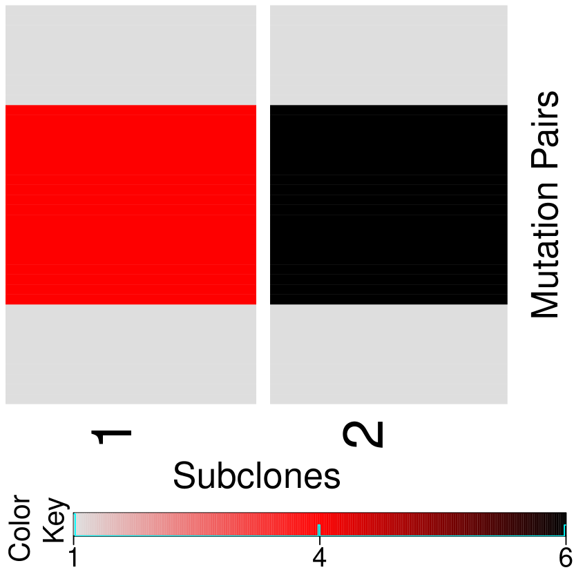
(a) Simu. 1, $\bm{Z}^{\text{TRUE}}$

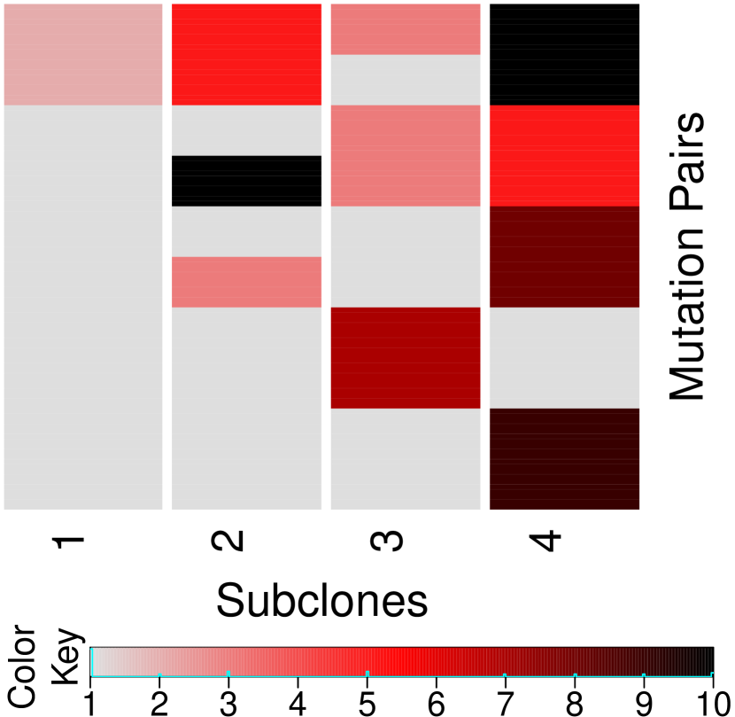
(b) Simu. 2, $\bm{Z}^{\text{TRUE}}$

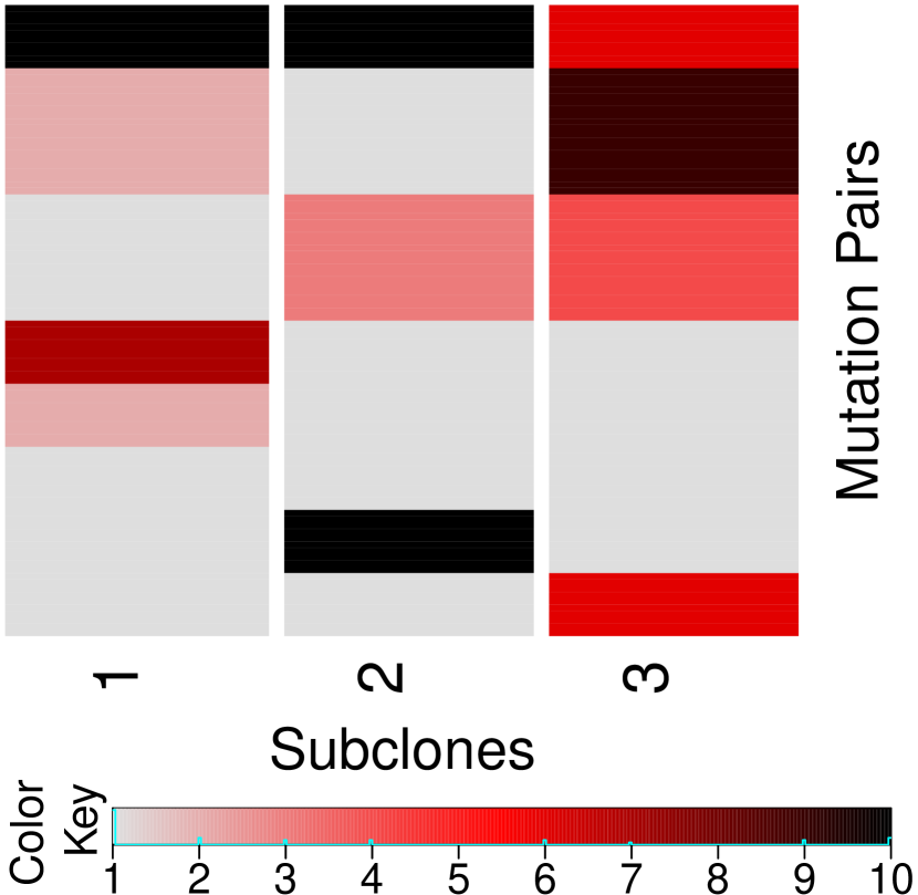
(c) Simu. 3, $\bm{Z}^{\text{TRUE}}$

(d) Simu. 1, $\hat{\bm{Z}}$

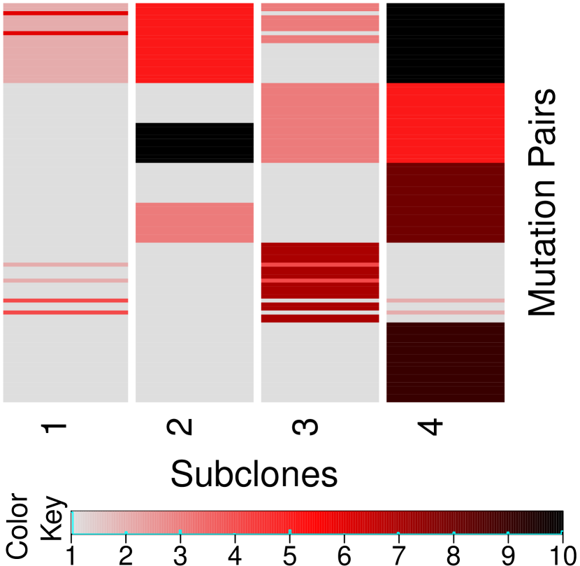
(e) Simu. 2, $\hat{\bm{Z}}$

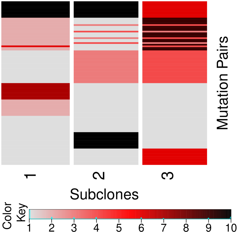
(f) Simu. 3, $\hat{\bm{Z}}$

Figure 2: Summary of simulation results. Simulation truth $\bm{Z}^{\text{TRUE}}$ (a, b, c), and posterior inference under PairClone (d, e, f) conditional on posterior modes of $C$.

5 PairClone Extensions

5.1 Incorporating Marginal Read Counts

Most somatic mutations are not part of the paired reads that we use in PairClone. We refer to these single mutations as SNVs (single nucleotide variants) and consider the following simple extension to incorporate marginal counts for SNVs in PairClone. We introduce a new $S\times C$ matrix $\bm{Z}^{S}$ to represent the genotype of the $C$ subclones for these additional SNVs. To avoid confusion, we denote the earlier $K\times C$ subclone matrix by $\bm{Z}^{P}$ in this section. The $(s,c)$ element of $\bm{Z}^{S}$ reports the genotype of SNV $s$ in subclone $c$, with $z^{S}_{sc}\in\{0,0.5,1\}$ denoting homozygous wild-type ($0$), heterozygous variant ($0.5$), and homozygous variant ($1$), respectively. The $c$-th column of $\bm{Z}^{P}$ and $\bm{Z}^{S}$ together define subclone $c$. We continue to assume copy number neutrality in all SNVs and mutation pairs (we discuss an extension to incorporating subclonal copy number variations in the next subsection). The marginal read counts are easiest incorporated in the PairClone model by recording them as right (or left) missing reads (as described in Section 2.1) for hypothetical pairs, $k=K+1,\ldots,k+S$. Let $\tilde{N}_{ts}$ and $\tilde{n}_{ts}$ denote the total count and the number of reads bearing a variant allele, respectively, for SNV $s$ in sample $t$. Treating $s$ as a mutation pair $k=K+s$ with missing second read, we record $n_{tk8}=\tilde{n}_{ts}$, $n_{tk1}=\ldots=n_{tk7}=0$ and $N_{tk}=\tilde{N}_{ts}$. We then proceed as before, now with $K+S$ mutation pairs. Inference reports an augmented $(K+S)\times C$ subclone matrix $\tilde{\bm{Z}}^{P}$. We record the first $K$ rows of $\tilde{\bm{Z}}^{P}$ as $\bm{Z}^{P}$, and transform the remaining $S$ rows to $\bm{Z}^{S}$ by only recording the genotypes of the observed loci.

We evaluate the proposed modeling approach with a simulation study. The simulation setting is the same as simulation 3 in Section 4, except that we discard the phasing information of mutation pairs $51-100$ and only record their marginal read counts. Figure 3(a)–(f) summarizes the simulation results. Panels (a, b) show the simulation truth for the mutation pairs and SNVs, respectively. Panel (c) shows the posterior $p(C\mid\bm{n}^{\prime\prime})$ and panels (d, e) show the estimated genotypes $\hat{\bm{Z}}^{P}$ and $\hat{\bm{Z}}^{S}$. Inference for the weights $w_{tc}$ recovers the simulation truth (not shown). The result compares favorably to inference under BayClone (Figure A.6 in the appendix), due to the additional phasing information for the first 50 mutation pairs.

For a direct evaluation of the information in the additional marginal counts we also evaluate posterior inference with only the first 50 mutation pairs, shown in Figure 3 (c, f). Comparison with Figure 3 (c, d) shows that the additional marginal counts do not noticeably improve inference on tumor heterogeneity.

Simulation truth

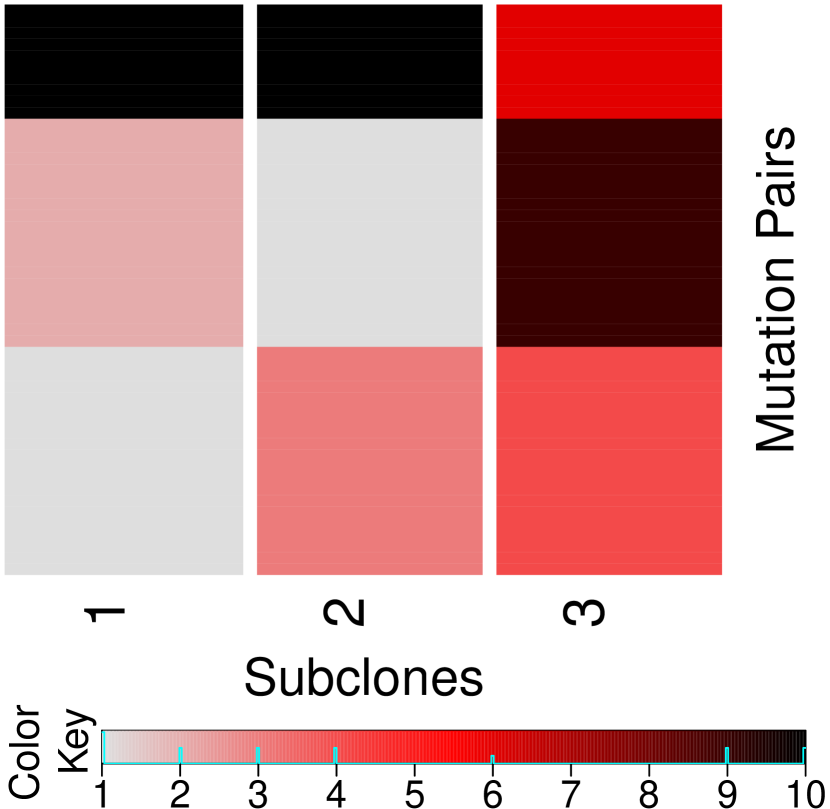
(a) $\bm{Z}^{P,\text{TRUE}}$

(b) $\bm{Z}^{S,\text{TRUE}}$

(c) $p_{b}(C\mid\bm{n}^{\prime\prime})$

Pairs and SNVs

Pairs only

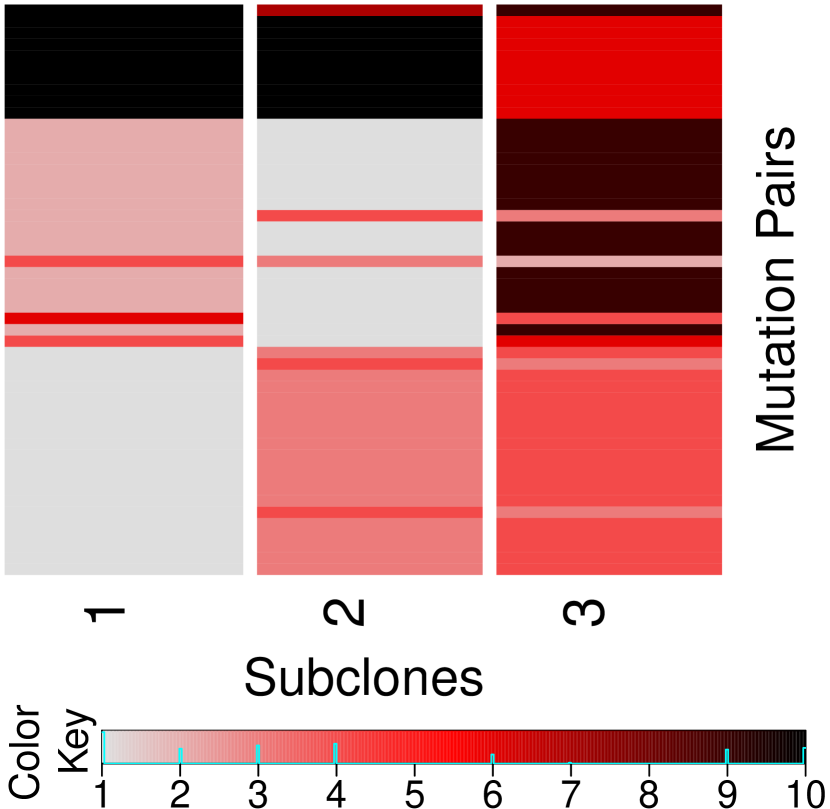
(d) $\hat{\bm{Z}}^{P}$

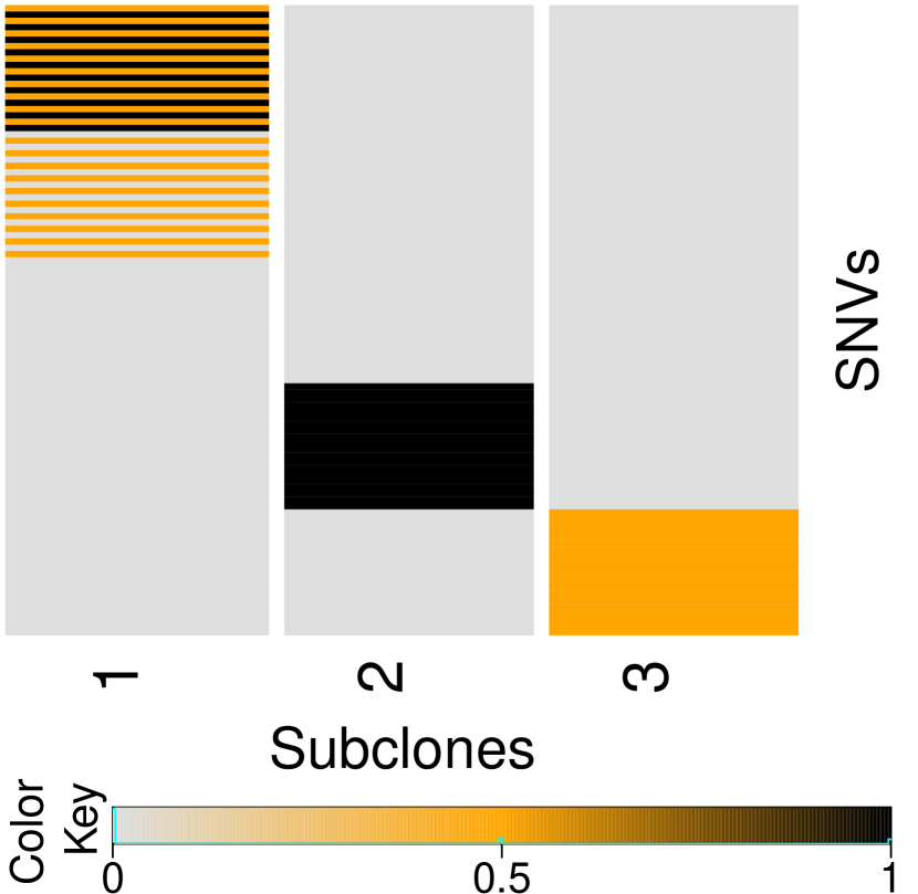
(e) $\hat{\bm{Z}}^{S}$

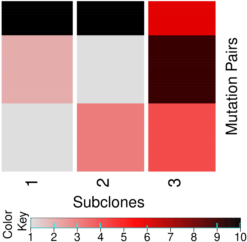
(f) $\hat{\bm{Z}}_{\text{wom}}^{P}$

Figure 3: Summary of simulation results using additional marginal read counts. Simulation truth $\bm{Z}^{P,\text{TRUE}}$ and $\bm{Z}^{S,\text{TRUE}}$ (a, b), posterior inference with marginal read counts incorporated (c, d, e), and posterior inference without marginal read counts (c, f).

5.2 Incorporating Tumor Purity

Usually, tumor samples are not pure in the sense that they contain certain proportions of normal cells. Tumor purity refers to the fraction of tumor cells in a tumor sample. To explicitly model tumor purity, we introduce a normal subclone, the proportion of which in sample $t$ is denoted by $w_{t\star}$, $t=1,\ldots,T$. The normal subclone does not possess any mutation (since we only consider somatic mutations). The tumor purity for sample $t$ is thus $(1-w_{t\star})$. The normal subclone is denoted by $\bm{z}_{*}$, with $\bm{z}_{k*}=\bm{z}^{(1)}$ for all $k$. The remaining subclones are still denoted by $\bm{z}_{c}$, $c=1,\ldots,C$, with proportion $w_{tc}$ in sample $t$, and $\sum_{c=0}^{C}w_{tc}+w_{t\star}=1$.

The probability model needs to be slightly modified to accommodate the normal subclone. The sampling model remains unchanged as (1). Same for the prior models for $\bm{Z}$, $\bm{\rho}$ and $C$. We only change the construction of $\tilde{p}_{tkg}$ and $p(\bm{w})$ as follows. With a new normal subclone, the probability of observing a short read $\bm{h}_{g}$ becomes $\tilde{p}_{tkg}=\sum_{c=1}^{C}w_{tc}\,A(\bm{h}_{g},\bm{z}_{kc})+w_{t\star}\,A(\bm{h}_{g},\bm{z}^{(1)})+w_{t0}\,\rho_{g},$ based on the same generative model described in Section 2.2. Let $\tilde{w}_{tc}=w_{tc}/(1-w_{t\star})$. We use a Beta-Dirichlet prior, $w_{t\star}\stackrel{{\scriptstyle iid}}{{\sim}}\mbox{Be}(d_{1}^{*},d_{2}^{*})$, and $\tilde{\bm{w}}_{t}\stackrel{{\scriptstyle iid}}{{\sim}}\mbox{Dir}(d_{0}$, $d$, $\ldots$, $d)$. An informative prior for $w_{t\star}$ could be based on an estimate from a purity caller, for example, Van Loo et al. (2010) or Carter et al. (2012).

We evaluate the modified model with a simulation study. The simulation setting is the same as simulation 3 in Section 4, except that we substitute the first subclone with a normal subclone. Posterior inference (not shown) recovers the simulation truth, with posterior mode $\hat{C}=2$. Inference on $\bm{Z}$ almost perfectly recovers the simulation truth shown in Figure 2(c) (with the first column replaced by an all normal “subclone”). Similarly for $\bm{w}$. See Appendix A.4 for details.

5.3 Incorporating Copy Number Changes

Tumor cells not only harbor sequence mutations such as SNVs and mutation pairs, they often undergo copy number changes and produce copy number variants (CNVs). Genomic regions with CNVs have copy number $\neq 2$. We briefly outline an extension of PairClone that includes CNVs in the inference. In addition to $\bm{Z}$ which describes sequence variation we introduce a $K\times C$ matrix $\bm{L}$ to represent subclonal copy number variation with $\ell_{kc}$ reporting the copy number for mutation pair $k$ in subclone $c$. We use $\bm{L}$ to augment the sampling model to include the total read count $N_{tk}$. Earlier in (1), the multinomial sample size $N_{tk}$ was considered fixed. We now add a sampling model. Following Lee et al. (2016) we assume

$$N_{tk}\mid\phi_{t},M_{tk}\sim\text{Poisson}(\phi_{t}M_{tk}/2)$$

Here, $\phi_{t}$ is the expected number of reads in sample $t$ under copy-neutral conditions, and $M_{tk}$ is a weighted average copy number across subclones,

$$M_{tk}=\sum_{c=1}^{C}w_{tc}\ell_{kc}+w_{t0}\ell_{k0}.$$

The last term $w_{t0}\ell_{k0}$ accounts for noise and artifacts, where $w_{t0}$ and $\ell_{k0}$ are the population frequency and copy number of the background subclone, respectively. We assume no CNVs for the background subclone, that is, $\ell_{k0}=2$ for all $k$. We complete the model with a prior $p(\bm{L})$. Assuming $\ell_{kc}\in\{0,\ldots,Q\}$, i.e., a maximum copy number $Q$, we use another instance of a finite cIBP. For each column of $\bm{L}$, we introduce $\bm{\pi}_{c}=(\pi_{c0},\pi_{c1},\ldots,\pi_{cQ})$ and assume $p(\ell_{kc}=q)=\pi_{cq}$, again with a Beta-Dirichlet prior for $\bm{\pi}_{c}$.

Recall the construction of $\tilde{p}_{tkg}$ in (3), including in particular the generative model. This generative model is now updated to include the varying $\ell_{tc}$. To generate a short read for mutation pair $k$, we first select a subclone $c$ from which the read arises, using the population frequencies $w_{tc}\ell_{kc}/\sum_{c=0}^{C}w_{tc}\ell_{kc}$ for sample $t$. Next we select with probability $z_{kcj}/\ell_{kc}$ one of the four possible alleles, $\bm{h}_{g}$, $g=1,2,3$ or $4$, where we now use $\bm{z}_{kc}=(z_{kcj},j=1,\ldots,4)$ to denote numbers of alleles having genotypes $00$, $01$, $10$ or $11$, and $\sum_{j}z_{kcj}=\ell_{kc}$. In the case of left (or right) missing locus we observe $\bm{h}_{g}$, $g=5$ or $6$ (or $g=7$ or $8$), corresponding to the observed locus of the chosen allele, similar to before. In summary, the probability of observing a short read $\bm{h}_{g}$ can be written as

$$\tilde{p}_{tkg}=\sum_{c=0}^{C}\left[\frac{w_{tc}\ell_{kc}}{\sum_{c=1}^{C}w_{tc}\ell_{kc}+w_{t0}\ell_{k0}}\cdot\frac{A(\bm{h}_{g},\bm{z}_{kc})}{\ell_{kc}}\right]=\frac{\sum_{c=0}^{C}w_{tc}A(\bm{h}_{g},\bm{z}_{kc})}{M_{tk}},$$

where $A(\cdot)$ corresponds to the described generative model.

6 Lung Cancer Data

6.1 Using PairClone

We apply PairClone to analyze whole-exome in-house data. Whole-exome sequencing data is generated from four ($T=4$) surgically dissected tumor samples taken from a single patient diagnosed with lung adenocarcinoma. The resected tumor is divided into two portions. One portion is flash frozen and another portion is formalin fixed and paraffin embedded (FFPE). Four different samples (two from each portion) are taken. DNA is extracted from all four samples. Agilent SureSelect v5+UTR probe kit (targeting coding regions plus UTRs) is used for exome capture. The exome library is sequenced in paired-end fashion on an Illumina HiSeq 2000 platform. About 60 million reads are obtained in FASTQ file format, each of which is 100 bases long. We map paired-end reads to the human genome (version HG19) (Church et al., 2011) using BWA (Li and Durbin, 2009) to generate BAM files for each individual sample. After mapping the mean coverage of the samples is around $70$ fold. We call variants using UnifiedGenotyper from GATK toolchain (McKenna et al., 2010) and generate a single VCF file for all of them. A total of nearly $115,000$ SNVs and small indels are called within the exome coordinates.

Next, using LocHap (Sengupta et al., 2015) we find mutation pair positions, the number of alleles and number of reads mapped to them. LocHap searches for multiple SNVs that are scaffolded by the same pair-end reads, that is, they can be recorded on one paired end read. We refer to such sets of multiple SNV’s as local haplotypes (LH). When more than two genotypes are exhibited by an LH, it is called a LH variant (LHV). Using individual BAM files and the combined VCF file, LocHap generates four individual output file in HCF format (Sengupta et al., 2015). An HCF file contains LHV segments with two or three SNV positions. In this analysis, we are only interested in mutation pair, and therefore filter out all the LHV segments consisting of more than two SNV locations. We restrict our analysis to copy number neutral regions. To further improve data quality, we drop all LHVs where two SNVs are very close to each other (within, say, $50$ bps) or close to any type of structural variants such as indels. We also remove those LHVs where either of the SNVs is mapped with strand bias by most reads, or either of the SNVs is mapped towards the end of the most aligned reads. Finally, we only consider mutation pairs that have strong evidence of heterogeneity. Since LHVs exhibit $>2$ genotypes in the short reads, by definition they are somatic mutations.

At the end of this process, $69$ mutation pairs are left and we record the read data from HCF files for the analysis. In addition, in the hope of utilizing more information from the data, we randomly choose 69 un-paired SNVs and include them in the analysis. Since in practice, tumor samples often include contamination with normal cells, we incorporate inference for tumor purity as described in Section 5.2. We run MCMC simulation for $30,000$ iterations, discarding the first $10,000$ iterations as initial burn-in and keeping every 10th MCMC sample. We set the hyperparameter exactly as in the simulation study of Section 5.2.

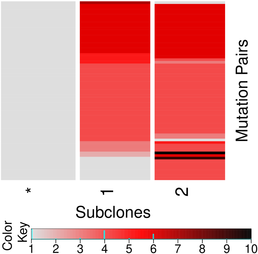
(a) $\hat{\bm{Z}}^{P}$

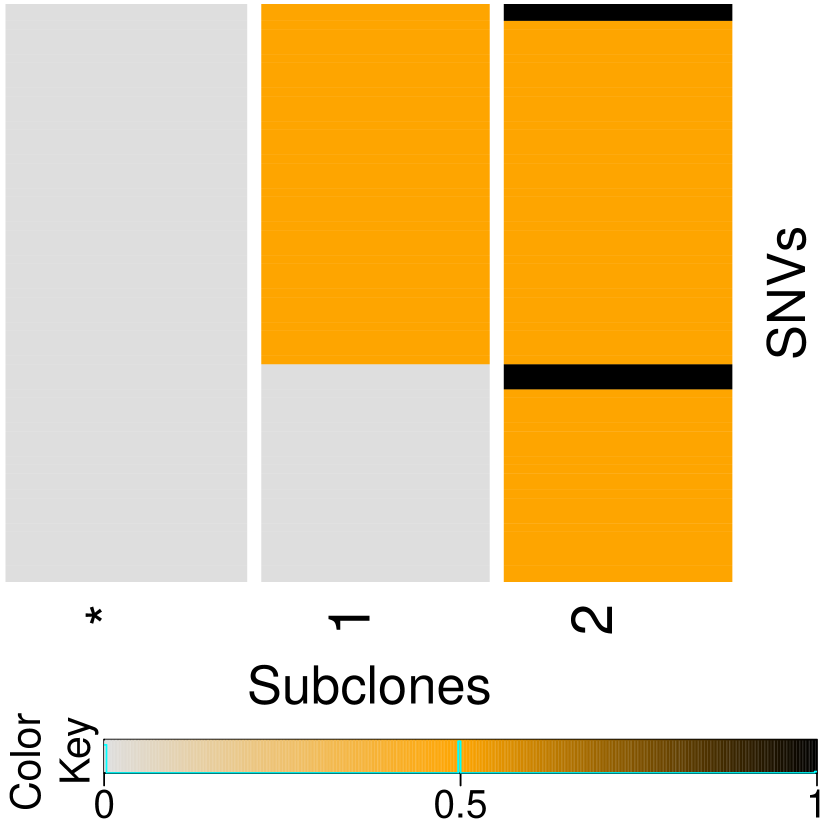
(b) $\hat{\bm{Z}}^{S}$

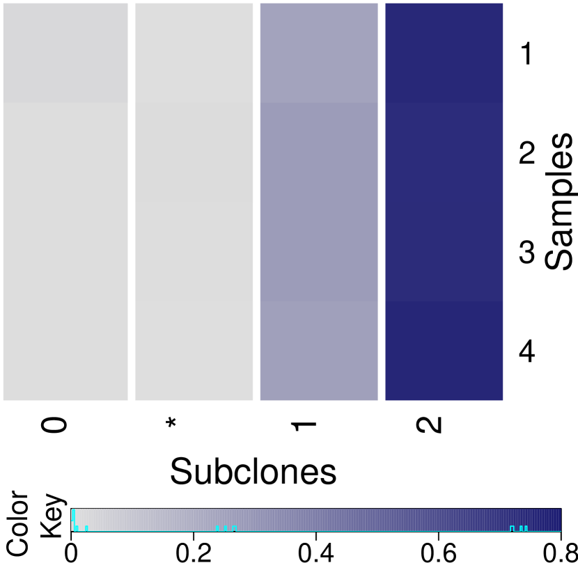
(c) $\hat{\bm{w}}$

Figure 4: Lung cancer. Posterior inference under PairClone.

Results

The posterior distribution $p_{b}(C\mid\bm{n}^{\prime\prime})$ (shown in Appendix Figure 9(a)) reports $p_{b}(C\mid\bm{n}^{\prime\prime})=0.24$, $0.31$, $0.17$ and $0.12$ for $C=1$, $2$, $3$ and $4$, respectively, and then quickly drops below $0.1$, with posterior mode $\hat{C}=2$. This means, excluding the effect of normal cell contamination, the tumor samples have two subclones. Figure 4(a, b) show the estimated subclone matrix $\hat{\bm{Z}}^{P}$ and $\hat{\bm{Z}}^{S}$ corresponding to mutation pairs and SNVs, respectively. The first column of $\hat{\bm{Z}}^{P}$ and $\hat{\bm{Z}}^{S}$ represents the normal subclone. The rows for both matrices are reordered for a better display. Figure 4(c) shows the estimated subclone proportions $\hat{\bm{w}}$ for the four samples. The second column of $\hat{\bm{w}}$ represents the proportions of normal subclones in the four samples. The small values indicate high purity of the tumor samples. The similar proportions across the four samples reflect the spatial proximity of the samples. Furthermore, excluding a few exceptions that might be due to model mis-fitting, the subclones form a simple phylogenetic tree: $*\rightarrow 1\rightarrow 2$. Subclones 1 and 2 share a large portion of common mutations, while subclone 2 has some private mutations that are missing in subclone 1.

For informal model checking we inspect a histogram of realized residuals (Appendix Figure 9(b)). To define residuals, we calculate estimated multinomial probabilities $\{\hat{p}_{tkg}\}$ according to $\hat{\bm{Z}}$, $\hat{\bm{w}}$ and empirical values of $\{v_{tk1},v_{tk2},v_{tk3}\}$. Let $\bar{p}_{tkg}=n_{tkg}/N_{tk}$. The figure plots the residuals $(\hat{p}_{tkg}-\bar{p}_{tkg})$. The resulting histogram of residuals is centered around zero with little mass beyond $\pm 0.04$, indicating a good model fit.

6.2 Using SNVs only

For comparison, we also run BayClone and PyClone on the same dataset. Using the log pseudo marginal likelihood (LPML), BayClone reports $\hat{C}=4$ subclones. The estimated subclone matrix in BayClone’s format is shown in Figure 5(a), with the rows reordered in the same way as in Figure 4(a, b). In light of the earlier simulation results we believe that the inference under PairClone is more reliable. Figure 5(b) shows the estimated subclone proportions under BayClone. Figure 5(c) shows the estimated clustering of the SNV loci under PyClone (the color coding along the axes). PyClone identifies 6 different clusters. The largest cluster (shown in brown) corresponds to loci that have heterozygous variants in both subclones 1 and 2, the second-largest cluster (shown in blueish green) corresponds to loci that have homozygous wild types in subclone 1 and homozygous variants in subclone 2, and the other smaller clusters represent other less common combinations. The clusters match with clustering of rows of $\hat{\bm{Z}}^{P}$ and $\hat{\bm{Z}}^{S}$. PyClone does not immediately give inference on subclones, but combing clusters with similar cellular prevalence across samples one is able to conjecture subclones. In this sense, PyClone gives similar result compared with PairClone. Finally, Figure 5(d) displays PyClone’s estimated cellular prevalences of clusters across different samples. The estimated subclone proportions and cellular prevalences across the four samples remain very similar also under the BayClone and PyClone output, which strengthens our inference that the four samples possess the same subclonal profile, each with two subclones.

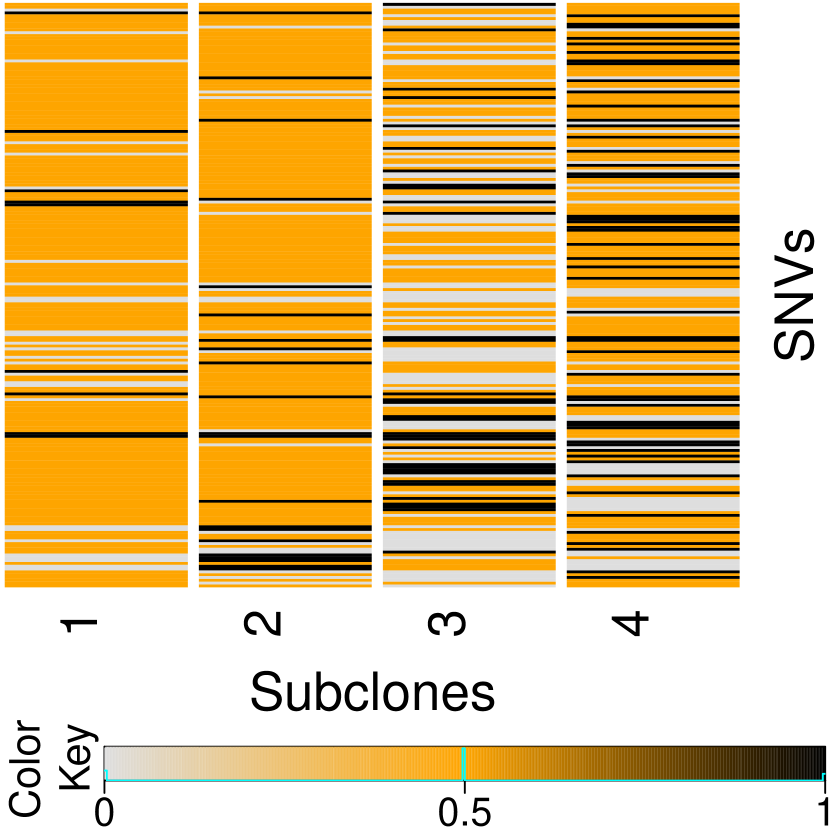
(a) $\hat{\bm{Z}}_{\text{BC}}$

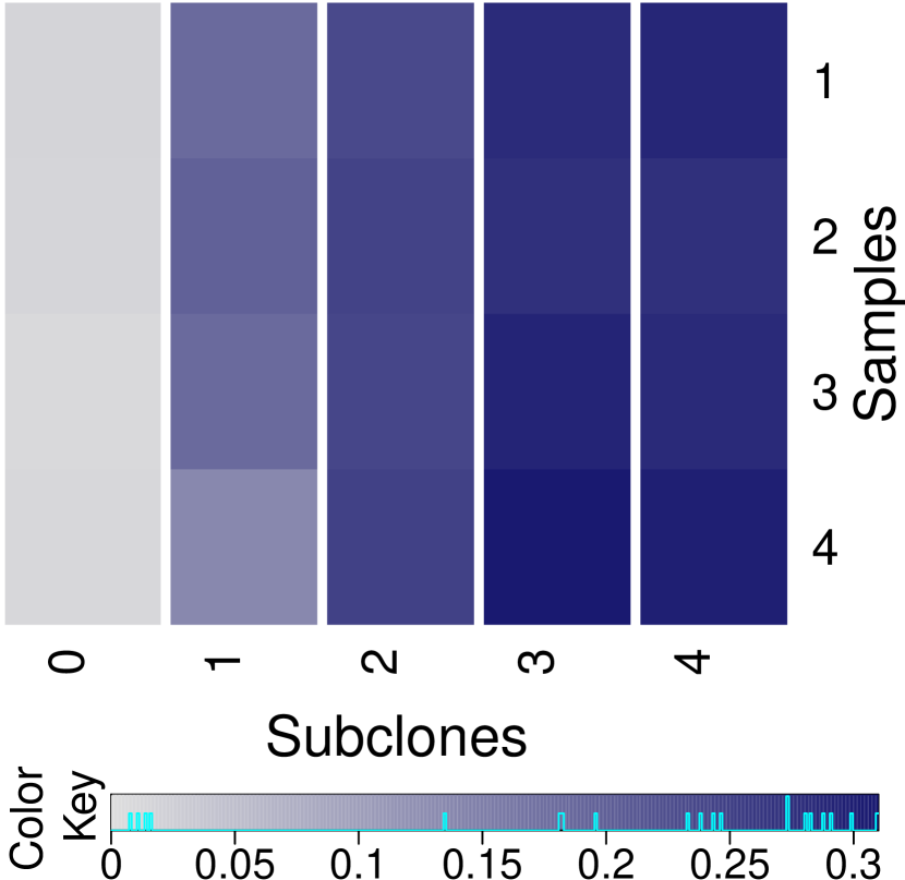
(b) $\hat{\bm{w}}_{\text{BC}}$

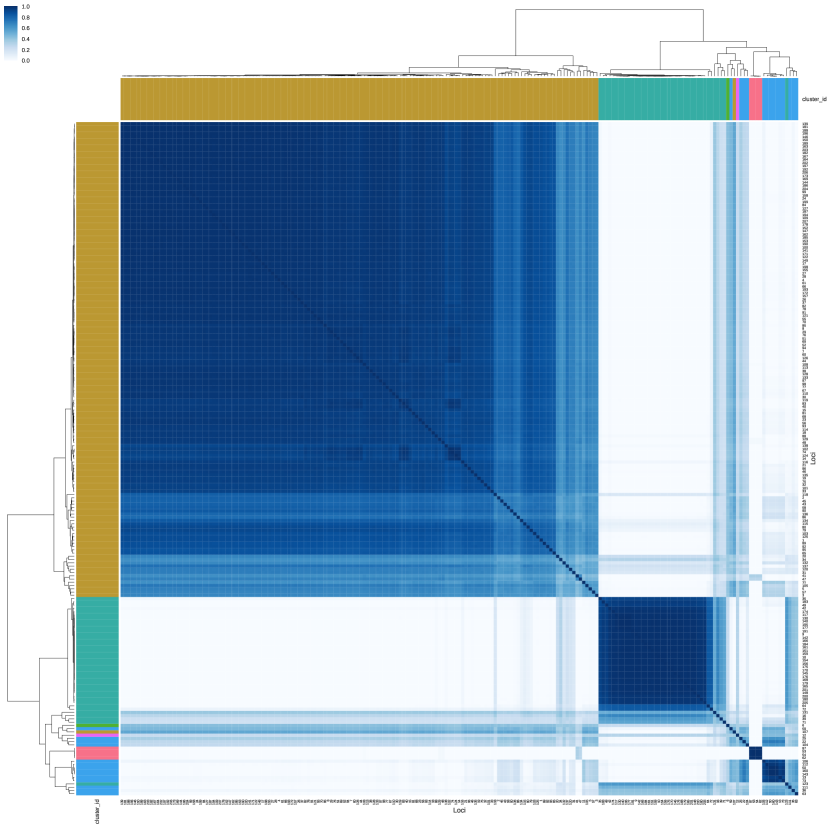
(c) Clustering matrix

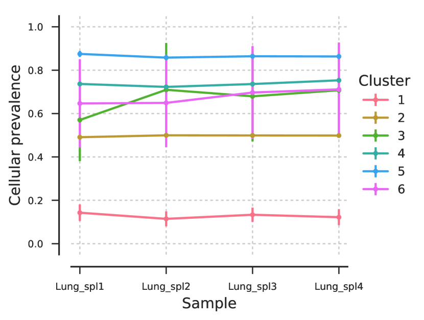
(d) Cellular prevalence

Figure 5: Lung cancer. Posterior inference under BayClone (a, b) and PyClone (c, d).

For another comparison, we run PyClone with a much larger number of SNVs ($S=1800$, which include the 69 pairs and 69 SNVs we ran analysis before) to evaluate the information gain by using additional marginal counts. The results are summarized in Figure 6, with panel (a) showing the estimated clustering of the 1800 SNVs. PyClone reports 34 clusters. The two largest clusters (olive and green clusters) in Panel (a) match with the two largest clusters (brown and bluish green clusters) in Figure 5(c) and also corroborate the two subclones inferred by PairClone. In addition, PyClone infers lots of noisy tiny clusters using 1800 SNVs, which we argue model only noise. In summary, this comparison shows the additional marginal counts do not noticeably improve inference on tumor heterogeneity, and modeling mutation pairs is a reasonable way to extract useful information from the data.

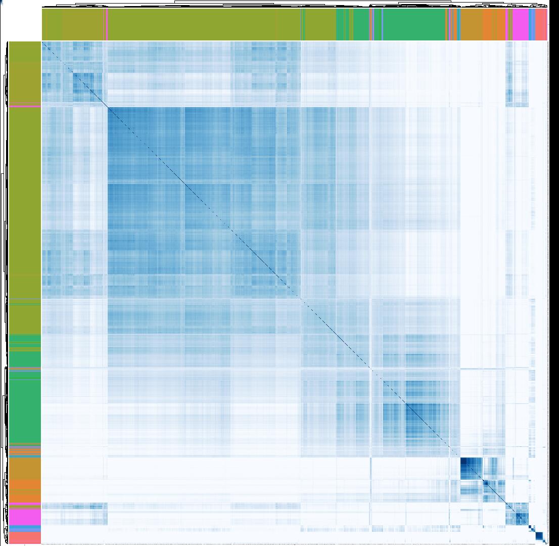
(a) Clustering matrix

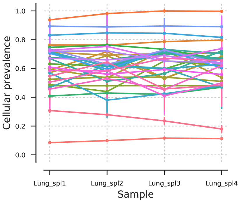
(b) Cellular prevalence

Figure 6: Lung cancer. Posterior inference under PyClone using 1800 SNVs. PyClone inferred 34 clusters with two major clusters (olive and green) and many small noisy clusters (other colors).

7 Conclusions

We can significantly enrich our understanding of cancer development by using high throughput NGS data to infer co-existence of subpopulations which are genetically different across tumors and within a single tumor (inter and intra tumor heterogeneity, respectively). In this paper, we have presented a novel feature allocation model for reconstructing such subclonal structure using mutation pair data. Proposed inference explicitly models overlapping mutation pairs. We have shown that more accurate inference can be obtained using mutation pairs data compared to using only marginal counts for single SNVs. Short reads mapped to mutation pairs can provide direct evidence for heterogeneity in the tumor samples. In this way the proposed approach is more reliable than methods for subclonal reconstruction that rely on marginal variant allele fractions only.

The proposed model is easily extended for data where an LH segment consists of more than two SNVs. We can easily accommodate $n$-tuples instead of pairs of SNVs by increasing the number of categorical values ($Q$) that the entries in the $\bm{Z}$ matrix can take. There are several more interesting directions of extending the current model. For example, one could account for the potential phylogenetic relationship among subclones (i.e the columns in the $\bm{Z}$ matrix). Such extensions would enable one to infer mutational timing and allow the reconstruction of tumor evolutionary histories.

Lastly, we focus on statistical inference using bulk sequencing data on tumor samples. Alternatively, biologists can apply single-cell sequencing on each tumor cell and study its genome one by one. This is a gold standard that can examine tumor heterogeneity at the single-cell level. However, single-cell sequencing is still expensive and cannot scale up. Also, many bioinformatics and statistical challenges are unmet in analyzing single-cell sequencing data.

Appendix A

A.1 MCMC Implementation Details

We first introduce $\theta_{tc}$ as an unscaled abundance level of subclone $c$ in sample $t$. Assume $\theta_{t0}\sim\text{Gamma}(d_{0},1)$ and $\theta_{tc}\mid C\sim\text{Gamma}(d,1)$. Let $w_{tc}=\theta_{tc}/\sum_{c^{\prime}=0}^{C}\theta_{tc^{\prime}}$, then $\bm{w}_{t}\sim\text{Dirichlet}(d_{0},d,\ldots,d)$. We make inference on $\bm{\theta}$ instead of $\bm{w}$ as the value of $\bm{\theta}$ is not restricted in a $C$-simplex. Similarly, we introduce $\rho_{g}^{*}$ as an unscaled version of $\rho_{g}$. We let $\rho_{g}^{*}\sim\text{Gamma}(d_{1},1)$ and $\rho_{g}=\rho_{g}^{*}/\sum_{g^{\prime}=1}^{4}\rho_{g^{\prime}}^{*}$ for $g=1,\ldots,4$, $\rho_{g}^{*}\sim\text{Gamma}(2d_{1},1)$ and $\rho_{g}=\rho_{g}^{*}/\sum_{g^{\prime}=5}^{6}\rho_{g^{\prime}}^{*}$ for $g=5,6$, and $\rho_{g}^{*}\sim\text{Gamma}(2d_{1},1)$ and $\rho_{g}=\rho_{g}^{*}/\sum_{g^{\prime}=7}^{8}\rho_{g^{\prime}}^{*}$ for $g=7,8$.

Conditional on $C$, the posterior distribution for the other parameters is given by

$$p(\bm{Z},\bm{\pi},\bm{\theta},\bm{\rho}^{*}\mid\bm{n},C)\propto\prod_{t=1}^{T}\prod_{k=1}^{K}\prod_{g=1}^{G}\tilde{p}_{tkg}^{n_{tkg}}\times\prod_{c=1}^{C}\prod_{q=1}^{Q}\pi_{cq}^{m_{cq}}\times\prod_{c=1}^{C}\left[\pi_{c1}^{1-1}(1-\pi_{c1})^{\alpha/C-1}\cdot\prod_{q=2}^{Q}\tilde{\pi}_{cq}^{\beta-1}\right]\times\\ \prod_{t=1}^{T}\left[\theta_{t0}^{d_{0}-1}e^{-\theta_{t0}}\prod_{c=1}^{C}\left(\theta_{tc}^{d-1}e^{-\theta_{tc}}\right)\right]\times\prod_{g=1}^{4}\left(\rho_{g}^{*d_{1}-1}e^{-\rho_{g}^{*}}\right)\cdot\prod_{g=5}^{8}\left(\rho_{g}^{*2d_{1}-1}e^{-\rho_{g}^{*}}\right).$$ (5)

where $m_{cq}=\sum_{k=1}^{K}I(\bm{z}_{kc}=\bm{z}^{(q)})$ counts the number of mutation pairs in subclone $c$ having genotype $\bm{z}^{(q)}$.

Updating $\bm{Z}$.

We update $\bm{Z}$ by sampling each $\bm{z}_{kc}$ from:

$$p(\bm{z}_{kc}=\bm{z}^{(q)}\mid\ldots)\propto\prod_{t=1}^{T}\prod_{g=1}^{G}\left[\sum_{c^{\prime}=1,c^{\prime}\neq c}^{C}w_{tc^{\prime}}\,A(\bm{h}_{g},\bm{z}_{kc^{\prime}})+w_{tc}\,A(\bm{h}_{g},\bm{z}^{(q)})+w_{t0}\,\rho_{g}\right]^{n_{tkg}}\cdot\pi_{cq}$$

Updating $\bm{\pi}$.

The posterior distribution for $\bm{\pi}$ is

$$p(\bm{\pi}\mid\ldots) \propto\prod_{c=1}^{C}\left[\left(\prod_{q=1}^{Q}\pi_{cq}^{m_{cq}}\right)\cdot\pi_{c1}^{1-1}(1-\pi_{c1})^{\alpha/C-1}\cdot\prod_{q=2}^{Q}\tilde{\pi}_{cq}^{\beta-1}\right]$$

$$=\prod_{c=1}^{C}\left[\pi_{c1}^{m_{c1}+1-1}(1-\pi_{c1})^{K-m_{c1}+\alpha/C-1}\cdot\prod_{q=2}^{Q}\tilde{\pi}_{cq}^{m_{cq}+\beta-1}\right].$$

For each $c=1,\ldots,C$, we update $\bm{\pi}_{c}$ by sampling from

$$\pi_{c1}\mid\ldots \sim\text{Beta}(m_{c1}+1,K-m_{c1}+\alpha/C),$$

$$(\tilde{\pi}_{c2},\ldots,\tilde{\pi}_{cQ})\mid\ldots \sim\text{Dirichlet}(m_{c2}+\beta,\ldots,m_{cQ}+\beta),$$

and transforming by $(\pi_{c2},\ldots,\pi_{cQ})=(1-\pi_{c1})\cdot(\tilde{\pi}_{c2},\ldots,\tilde{\pi}_{cQ})$.

Updating $\bm{\theta}$.

We update each $\theta_{tc}$ sequentially. For $c=1,\ldots,C$,

$$p(\theta_{tc}\mid\ldots)\propto\prod_{k=1}^{K}\prod_{g=1}^{G}\left[\sum_{c=1}^{C}w_{tc}\,A(\bm{h}_{g},\bm{z}_{kc})+w_{t0}\,\rho_{g}\right]^{n_{tkg}}\cdot\theta_{tc}^{d-1}e^{-\theta_{tc}}.$$

A Metropolis-Hastings transition probability is used to update $\theta_{tc}$. At each iteration, we propose a new $\tilde{\theta}_{tc}$ (on the log scale) by $\log(\tilde{\theta}_{tc})\sim N(\log\theta_{tc},0.2)$, and evaluate the acceptance probability by $p_{\text{acc}}(\theta_{tc},\tilde{\theta}_{tc})=1\wedge\left[\left(p(\tilde{\theta}_{tc}\mid\ldots)\,p(\theta_{tc}\mid\tilde{\theta}_{tc})\right)\middle/\left(p(\theta_{tc}\mid\ldots)\,p(\tilde{\theta}_{tc}\mid\theta_{tc})\right)\right]$. The term $p(\theta_{tc}\mid\tilde{\theta}_{tc})/p(\tilde{\theta}_{tc}\mid\theta_{tc})=\tilde{\theta}_{tc}/\theta_{tc}$ takes into account the Jacobian of the log transformation. For $c=0$, the only difference is to substitute $d$ with $d_{0}$.

Updating $\bm{\rho}^{*}$.

We update each $\rho_{g}^{*}$ sequentially. For $g=1,\ldots,4$,

$$p(\rho_{g}^{*}\mid\ldots)\propto\prod_{t=1}^{T}\prod_{k=1}^{K}\prod_{g=1}^{G}\left[\sum_{c=1}^{C}w_{tc}\,A(\bm{h}_{g},\bm{z}_{kc})+w_{t0}\,\rho_{g}\right]^{n_{tkg}}\cdot\rho_{g}^{*d_{1}-1}e^{-\rho_{g}^{*}}.$$

A Metropolis-Hastings transition probability is used to update $\rho_{g}^{*}$. At each iteration, we propose a new $\tilde{\rho}_{g}^{*}$ (on the log scale) by $\log(\tilde{\rho}_{g}^{*})\sim N(\log{\rho_{g}^{*}},0.1)$, and evaluate the acceptance probability by $p_{\text{acc}}(\rho_{g}^{*},\tilde{\rho}_{g}^{*})=1\wedge\left[\left(p(\tilde{\rho}_{g}^{*}\mid\ldots)\,p(\rho_{g}^{*}\mid\tilde{\rho}_{g}^{*})\right)/\left(p(\rho_{g}^{*}\mid\ldots)\,p(\tilde{\rho}_{g}^{*}\mid\rho_{g}^{*})\right)\right]$. The term $p(\rho_{g}^{*}\mid\tilde{\rho}_{g}^{*})/p(\tilde{\rho}_{g}^{*}\mid\rho_{g}^{*})=\tilde{\rho}_{g}^{*}/\rho_{g}^{*}$ takes into account the Jacobian of the log transformation. For $g=4,\ldots,8$, the only difference is to substitute $d_{1}$ with $2d_{1}$.

Parallel tempering.

Parallel tempering (PT) is a MCMC technique first proposed by Geyer (1991). A good review can be found in Liu (2008). PT is suitable for sampling from a multi-modal state space. It helps the MCMC chain to move freely among local modes which is desired in our application, and to create a better mixing Markov chain.

Algorithm 1 Parallel Tempering

1:Draw initial state $(\bm{x}_{1}^{(0)},\ldots,\bm{x}_{I}^{(0)})$ from appropriate distributions

2:for $l$ in $1,\ldots,L$  do

3:     Draw $u\sim\text{Uniform}(0,1)$

4:     if $u\leq u_{0}$ then

5:         Conduct the parallel step: update every $\bm{x}_{i}^{(l)}$ to $\bm{x}_{i}^{(l+1)}$ via respective MCMC scheme

6:     else

7:         Conduct the swapping step: draw $i\sim\text{Discrete-Uniform}(1,\ldots,I-1)$, propose a swap between $\bm{x}_{i}^{(l)}$ and $\bm{x}_{i+1}^{(l)}$, accept the swap with probability

$$\min\left\{1,\frac{\pi_{i}(\bm{x}_{i+1}^{(l)})\pi_{i+1}(\bm{x}_{i}^{(l)})}{\pi_{i}(\bm{x}_{i}^{(l)})\pi_{i+1}(\bm{x}_{i+1}^{(l)})}\right\}$$

8:     end if

9:end for

To sample from the target distribution $\pi(\bm{x})$, we consider a family of distributions $\Pi=\{\pi_{i},i=1,\ldots,I\}$, where $\pi_{i}(\bm{x})\propto\pi(\bm{x})^{1/\Delta_{i}}$. Without loss of generality, let $\Delta_{I}=1$ and $\pi_{I}(\bm{x})=\pi(\bm{x})$. Denote by $\mathcal{X}_{i}$ the state space of $\pi_{i}(\bm{x})$. The PT scheme is illustrated in Algorithm 1.

In our application, we find by simulation that PT works well with $I=10$ temperatures and $\{\Delta_{1},\ldots,\Delta_{10}\}=\{4.5,3.2,2.5,2,1.7,1.5,1.35,1.2,1.1,1\}$. We therefore use this parameter setting for all the simulation studies as well as the lung cancer dataset.

A.2 Updating $C$

For updating $C$, we split the data into a training set $\bm{n}^{\prime}$, and a test set $\bm{n}^{\prime\prime}$ with $n_{tkg}^{\prime}=bn_{tkg}$ and $n_{tkg}^{\prime\prime}=(1-b)n_{tkg}$. Let $p_{b}(\bm{x}\mid C)=p(\bm{x}\mid\bm{n}^{\prime},C)$ denote the posterior of $\bm{x}$ conditional on $C$ evaluated on the training set only. We use $p_{b}$ in two occasions. First, we replace the original prior $p(\bm{x}\mid C)$ by $p_{b}(\bm{x}\mid C)$, and second, we use $p_{b}$ as a proposal distribution of $\tilde{\bm{x}}$ as $q(\tilde{\bm{x}}\mid\tilde{C})=p_{b}(\tilde{\bm{x}}\mid\tilde{C})$. We show that the use of the training sample posterior as proposal and modified prior in equation (4) (original manuscript) implies an approximation in the reported marginal posterior for $C$, but leaves the conditional posterior for all other parameters (given $C$) unchanged.

We evaluate the acceptance probability of $\tilde{C}$ on the test data by

$$p_{\text{acc}}(C,\bm{x},\tilde{C},\tilde{\bm{x}}) =1\wedge\frac{p(\bm{n}^{\prime\prime}\mid\tilde{\bm{x}},\tilde{C})}{p(\bm{n}^{\prime\prime}\mid\bm{x},C)}\cdot\frac{p(\tilde{C})p(\tilde{\bm{x}}\mid\bm{n}^{\prime},\tilde{C})}{p(C)p(\bm{x}\mid\bm{n}^{\prime},C)}\cdot\frac{q(C\mid\tilde{C})q(\bm{x}\mid C)}{q(\tilde{C}\mid C)q(\tilde{\bm{x}}\mid\tilde{C})}$$

$$=1\wedge\frac{p(\bm{n}^{\prime\prime}\mid\tilde{\bm{x}},\tilde{C})}{p(\bm{n}^{\prime\prime}\mid\bm{x},C)}\cdot\frac{p(\tilde{C})}{p(C)}.$$

Under the model $p_{b}(\cdot)$ with the modified prior, the implied conditional posterior on $\bm{x}$ satisfies

$$p_{b}(\bm{x}\mid C,\bm{n})=\frac{p_{b}(\bm{x}\mid C)p(\bm{n}^{\prime\prime}\mid\bm{x},C)}{\int p_{b}(\bm{x}\mid C)p(\bm{n}^{\prime\prime}\mid\bm{x},C)d\bm{x}}\\ =\frac{p(\bm{x}\mid C)p(\bm{n}^{\prime}\mid\bm{x},C)p(\bm{n}^{\prime\prime}\mid\bm{x},C)}{\int p(\bm{x}\mid C)p(\bm{n}^{\prime}\mid\bm{x},C)p(\bm{n}^{\prime\prime}\mid\bm{x},C)d\bm{x}}=p(\bm{x}\mid C,\bm{n}),$$

which indicates the conditional posterior of $\bm{x}$ remains entirely unchanged. The implied marginal posterior on $C$ is $p_{b}(C\mid\bm{n}^{\prime\prime})\propto p(C)\,p_{b}(\bm{n}^{\prime\prime}\mid C)$, with the likelihood on the test data evaluated as $p_{b}(\bm{n}^{\prime\prime}\mid C)=\int p(\bm{n}^{\prime\prime}\mid\bm{x},C)\,p_{b}(\bm{x}\mid C)d\bm{x}$. The use of the prior $p_{b}(\tilde{\bm{x}}\mid\tilde{C})$ is similar to the construction of the fractional Bayes factor (FBF) (O’Hagan, 1995). Let $\bm{u}=\{\bm{\pi},\bm{w},\bm{\rho}\}$ denote the parameters other than $\bm{Z}$ and let $\bm{u}^{*}$ denote the maximum likelihood estimate for $\bm{u}$. We follow O’Hagan (1995) to show that inference on $C$ is as if we were making use of only a fraction $(1-b)$ of the data, with a dimension penalty. In short,

$$p_{b}(C\mid\bm{n}^{\prime\prime})\propto p(C)p(\bm{n}\mid\bm{u}^{*},C)^{1-b}\,b^{\;p_{C}/2},$$

approximately, where $\bm{u}^{*}$ is the maximum likelihood estimate of $\bm{u}$, and $p_{C}$ is the number of unconstrained parameters in $\bm{u}$. To obtain this approximation, consider the marginal sampling model under $p_{b}(\cdot)$, after marginalizing with respect to $\bm{x}$:

$$p_{b}(\bm{n}^{\prime\prime}\mid C)=\int p(\bm{n}^{\prime\prime}\mid\bm{x},C)p_{b}(\bm{x}\mid C)d\bm{x}\\ =\int p(\bm{n}^{\prime\prime}\mid\bm{x},C)\,\frac{p(\bm{n}^{\prime}\mid\bm{x},C)p(\bm{x}\mid C)}{\int p(\bm{n}^{\prime}\mid\bm{x},C)p(\bm{x}\mid C)d\bm{x}}\,d\bm{x}=\frac{\int p(\bm{n}\mid\bm{x},C)p(\bm{x}\mid C)d\bm{x}}{\int p(\bm{n}^{\prime}\mid\bm{x},C)p(\bm{x}\mid C)d\bm{x}}.$$

Here we substituted the training sample posterior as (new) prior $p_{b}(\bm{x}\mid C)$. The integration includes a marginalization with respect to the discrete $\bm{Z}$,

$$\int p(\bm{n}\mid\bm{x},C)p(\bm{x}\mid C)d\bm{x} =\int\sum_{\bm{Z}}p(\bm{n}\mid\bm{Z},\bm{u},C)p(\bm{Z}\mid\bm{u},C)p(\bm{u}\mid C)d\bm{u}$$

$$=\int p(\bm{n}\mid\bm{u},C)p(\bm{u}\mid C)d\bm{u},$$

For the remaining real valued parameters $\bm{u}$ we use an appropriate one-to-one transformation (e.g. logit transformation) $\bm{u}\mapsto\tilde{\bm{u}}$, such that $\tilde{\bm{u}}$ is unconstrained. To simplify notation we continue to refer to the transformed parameter as $\bm{u}$ only. Next, under the binomial sampling model $p(\bm{n}^{\prime}\mid\bm{x},C)\propto p(\bm{n}\mid\bm{x},C)^{b}$, leading to

$$p_{b}(\bm{n}^{\prime\prime}\mid C) =\frac{\int p(\bm{n}\mid\bm{u},C)p(\bm{u}\mid C)d\bm{u}}{\int p(\bm{n}^{\prime}\mid\bm{u},C)p(\bm{u}\mid C)d\bm{u}}$$

$$=\underbrace{\frac{\left[\prod_{t,k}N_{tk}!/(n_{tk1}!\cdots n_{tkG}!)\right]^{b}}{\prod_{t,k}(bN_{tk})!/\left[(bn_{tk1})!\cdots(bn_{tkG})!\right]}}_{m(\bm{n})}\cdot\underbrace{\frac{\int p(\bm{n}\mid\bm{u},C)p(\bm{u}\mid C)d\bm{u}}{\int p(\bm{n}\mid\bm{u},C)^{b}p(\bm{u}\mid C)d\bm{u}}}_{h_{b}(\bm{n}\mid C)},$$

Let $m(\bm{n})$ and $h_{b}(\bm{n}\mid C)$ denote the two factors. The first, $m(\bm{n})$, is a constant term. And the second factor, $h_{b}(\bm{n}\mid C)$, has exactly the same form as equation (12) in O’Hagan (1995), who shows

$$h_{b}(\bm{n}\mid C)\approx p(\bm{n}\mid\bm{u}^{*},C)^{1-b}b^{\;p_{C}/2}$$

Let $N=\sum_{t,k}N_{tk}$. The argument of Gelfand and Dey (1994) (case (e)) suggests that the error in this approximation is of order $O(1/N^{2})$ (note that Gelfand and Dey use expansion around the M.A.P. while O’Hagan uses expansions around the M.L.E.). This establishes the stated approximation of the posterior $p_{b}(C\mid\bm{n}^{\prime\prime})\approx k\cdot p(C)p(\bm{n}\mid\bm{u}^{*},C)^{1-b}\,b^{\;p_{C}/2}$, approximately.

A.3 Simulation Studies and Comparison with Marginal Counts

We report details of the three simulation studies that are summarized in the manuscript (Section 4). The discussion includes a comparison with inference under methods that use only marginal mutation counts.

A.3.1 Simulation 1

Setup.

In the first simulation, we illustrate the advantage of using mutation pair data over marginal SNV counts. We generate hypothetical short reads data for $T=1$ sample and $K=40$ mutation pairs. Based on our own experiences, for a whole-exome sequencing data set, we usually obtain dozens of mutation pairs with decent coverage. See Sengupta et al. (2015) for a discussion. We assume there are $C^{\text{TRUE}}=2$ latent subclones, and set their population frequencies as $\bm{w}^{\text{TRUE}}=(1.0\times 10^{-7},0.8,0.2)$, where $1.0\times 10^{-7}$ refers to the proportion of the hypothetical background subclone $c=0$. The subclone matrix $\bm{Z}^{\text{TRUE}}$ is shown in Figure A.1(a) (as a heat map). Light grey, red and black colors are used to represent genotypes $\bm{z}^{(1)}$, $\bm{z}^{(4)}$ and $\bm{z}^{(6)}$. For example, subclone 1 has genotype $\bm{z}^{(1)}$ (wild type) for mutation pairs 1–10 and 31 – 40, and $\bm{z}^{(4)}$ for mutation pairs 11–30. We generate $\bm{\rho}^{\text{TRUE}}$ from its prior with hyperparameter $d_{1}=1$. Next we set the probabilities of observing left and right missing reads as $v_{tk2}=v_{tk3}=0.3$ for all $k$ and $t$, to mimic a typical missing rate observed in the real data. We calculate multinomial probabilities $\{p_{tkg}^{\text{TRUE}}\}$ shown in equations (3) and (2) from the simulated $\bm{Z}^{\text{TRUE}}$, $\bm{w}^{\text{TRUE}}$ and $\bm{\rho}^{\text{TRUE}}$. Total read counts $N_{tk}$ are generated as random numbers ranging from $400$ to $600$, and finally we generate read counts $n_{tkg}$ from the multinomial distribution given $N_{tk}$ as shown in equation (1).

We fit the model with hyperparameters fixed as follows: $\alpha=4$, $\gamma_{2}=\cdots=\gamma_{Q}=2$, $d=0.5$, $d_{0}=0.03$, $d_{1}=1$, and $r=0.4$. We set $C_{\text{min}}=1$ and $C_{\text{max}}=10$ as the range of $C$. The fraction $b$ needs to be calibrated. We choose $b$ such that the test sample size $(1-b)\sum_{t=1}^{T}\sum_{k=1}^{K}N_{tk}$ is approximately equal to $160/T$. See Section A.5 for a discussion of this choice.

We run MCMC simulation for $30,000$ iterations, discarding the first $10,000$ iterations as initial burn-in, and keep one sample every $10$ iterations. The initial values are randomly generated from the priors.

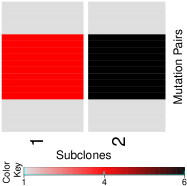
(a) $\bm{Z}^{\text{TRUE}}$	(b) $p_{b}(C\mid\bm{n}^{\prime\prime})$	(c) $\hat{\bm{Z}}$
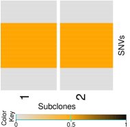
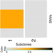
(d) Histogram of $(\hat{p}_{tkg}-p_{tkg}^{\text{TRUE}})$	(e) $\bm{Z}_{\text{BC}}^{\text{TRUE}}$	(f) $\hat{\bm{Z}}_{\text{BC}}$

Figure A.1: Simulation 1. Simulation truth $\bm{Z}^{\text{TRUE}}$ (a, e), and posterior inference under PairClone (b, c, d) and under BayClone (f).

Results.

Figure A.1(b) shows $p_{b}(C\mid\bm{n}^{\prime\prime})$, where the vertical dashed line marks the simulation truth. The posterior mode $\hat{C}=2$ recovers the truth. Figure A.1(c) shows the point estimate of $\bm{Z}^{\text{TRUE}}$, given by $\hat{\bm{Z}}$. The true subclone structure is perfectly recovered. The estimated subclone weights are $\hat{\bm{w}}=(2.27\times 10^{-116},0.8099,0.1901)$, which is also very close to the truth. We use $\hat{\bm{Z}}$ and $\hat{\bm{w}}$ to calculate estimated multinomial probabilities, denoted by $\{\hat{p}_{tkg}\}$. Figure A.1(d) shows a histogram of the differences $(\hat{p}_{tkg}-p_{tkg}^{\text{TRUE}})$ as a residual plot to assess model fitting. The histogram is centered at zero with little variation, indicating a reasonably good model fit. In summary, this simulation shows that the proposed inference can almost perfectly recover the truth in a simple scenario with a single sample.

Inference with marginal read counts.

We compare the proposed inference under PairClone versus inference under SNV-based subclone callers ,i.e., based on marginal (un-paired) counts of point mutations, including BayClone (Sengupta et al., 2015) and PyClone (Roth et al., 2014).

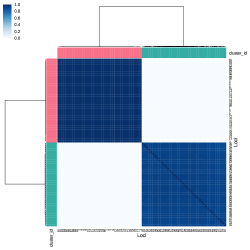
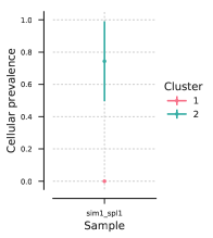
(a) Posterior similarity matrix	(b) Cellular prevalence

Figure A.2: Simulation 1. Posterior inference under PyClone.

BayClone infers the subclone structure based on marginal allele frequencies of the recorded SNVs, and chooses the number of subclones based on log pseudo marginal likelihood (LPML) model comparison. Under the LPML criterion, the estimated number of subclones reported by BayClone is $\hat{C}=2$, which also recovers the truth. Figure A.1(e) displays the true genotypes of the unpaired SNVs, denoted by $\bm{Z}_{\text{BC}}^{\text{TRUE}}$, based on the true genotypes in Figure A.1 for the mutation pairs. That is, we derive the corresponding marginal genotype for each SNV in the mutation pair based on the truth $\bm{Z}^{\text{TRUE}}$. Figure A.1(f) shows the heat map of estimated matrix $\hat{\bm{Z}}_{\text{BC}}$, where $z_{sc}=0$ (light grey), $0.5$ (orange) and $1$ (black) refer to homozygous wild-type, heterozygous variant and homozygous variant at SNV locus $s$, respectively. The estimated subclone proportions are $\hat{\bm{w}}_{\text{BC}}=(0.008,0.988,0.004)$.

PyClone, on the other hand, clusters mutations based on allele frequencies of the recorded SNVs using the implied clustering under a Dirichlet process mixture model. PyClone does not report subclonal genotypes and thus is not directly comparable with PairClone. Posterior inference is summarized in Figure A.2. Panel (a) indicates that the 80 SNV loci form two clusters, with one cluster corresponding to loci 1–20 and 61–80, and the other cluster corresponding to loci 21–60, which agrees with the truth. Panel (b) shows the cellular prevalence of the two clusters across samples, where the middle point represents the posterior mean, and the error bar indicates posterior standard deviation. The cellular prevalence is defined as fraction of clonal population harbouring a mutation. In the PyClone MCMC samples, the estimated cellular prevalence of cluster 2 fluctuates between 0.5 and 1 and thus includes high posterior uncertainty, while the true cellular prevalence of cluster 2 is 1.

The estimates under SNV-based subclone callers do not fully recover the simulation truth. The main reason is probably that the phasing information of paired SNVs is lost in the marginal counts that are used in BayClone and PyClone, making the subclone estimation less accurate than under PairClone. For example, the two subclones with genotypes $\bm{z}^{(4)}=(00,11)$ and $\bm{z}^{(6)}=(01,10)$ lead to exactly the same allele frequency (50%) for both loci. BayClone can not distinguish between these two different subclones based on the 50% allele frequency for each locus. Although BayClone correctly reports the number of subclones, inference mistakenly includes a normal subclone with negligible weight, and thus fails to recover the true population frequencies. On the other hand, PyClone can not identify if cluster 2 contains homozygous (corresponding to cellular prevalence of 0.5) or heterozygous (corresponding to cellular prevalence of 1) variants. In contrast, using the phasing information, PairClone is able to infer two subclones having genotypes $(00,11)$ and $(01,10)$ for mutation pairs 11–30, and we know cluster 2 contains only heterozygous variants for sure.

A.3.2 Simulation 2

In the second simulation, we consider data with $K=100$ mutation pairs and a more complicated subclonal structure with $C^{\text{TRUE}}=4$ latent subclones. We generate hypothetical data for $T=4$ samples. The subclone matrix $\bm{Z}^{\text{TRUE}}$ is shown in Figure A.3(a). Colors on a scale from light grey to red, to black (see the scale in the figure) are used to represent genotype $\bm{z}^{(q)}$ with $q=1,\ldots,10$. For example, subclone 4 has genotype $\bm{z}^{(10)}$ for mutation pairs 1–20, $\bm{z}^{(5)}$ for mutation pairs 21–40, $\bm{z}^{(8)}$ for mutation pairs 41–60, $\bm{z}^{(1)}$ for mutation pairs 61–80, and $\bm{z}^{(9)}$ for mutation pairs 81–100. For each sample $t$, we generate the subclone proportions from a Dirichlet distribution, $\bm{w}_{t}^{\text{TRUE}}\sim\mbox{Dir}(0.01,\sigma(20,10,5,2))$, where $\sigma(20,10,5,2)$ is a random permutation of $(20,10,5,2)$. The subclone proportion matrix $\bm{w}^{\text{TRUE}}$ is shown in Figure A.3(b), where darker blue color indicates higher abundance of a subclone in a sample, and light grey color represents low abundance. The parameters $\bm{\rho}^{\text{TRUE}}$ and $N_{tk}$ are generated using the same approach as before, and we use $v_{tk2}=v_{tk3}=0.3$ for $k=1,\ldots,50$ and all $t$, and $v_{tk2}=v_{tk3}=0.35$ for $k=51,\ldots,100$ and all $t$. Finally, we calculate $\{p_{tkg}^{\text{TRUE}}\}$ and generate read counts $n_{tkg}$ from equation (1) similar to previous simulation.

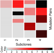
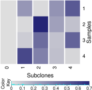
(a) $\bm{Z}^{\text{TRUE}}$	(b) $\bm{w}^{\text{TRUE}}$	(c) $p_{b}(C\mid\bm{n}^{\prime\prime})$
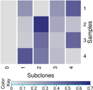
(d) $\hat{\bm{Z}}$	(e) $\hat{\bm{w}}$	(f) Histogram of $(\hat{p}_{tkg}-p_{tkg}^{\text{TRUE}})$

Figure A.3: Simulation 2. Simulation truth $\bm{Z}^{\text{TRUE}}$ and $\bm{w}^{\text{TRUE}}$ (a, b), and posterior inference under PairClone (c, d, e, f).

We fit the model with the same set of hyperparameters and MCMC parameters as in simulation 1. Figure A.3(c) shows $p_{b}(C\mid\bm{n}^{\prime\prime})$. Again, the posterior mode $\hat{C}=4$ recovers the truth. Figure A.3(d) shows the estimate $\hat{\bm{Z}}$; the truth is nicely approximated. Some mismatches are expected under this more complex subclone structure. The estimated subclone proportions $\hat{\bm{w}}$ are shown in Figure A.3(e), again close to the truth. Figure A.3(f) shows the histogram of ($\hat{p}_{tkg}-p_{tkg}^{\text{TRUE}}$) which indicates a good model fit.

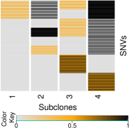
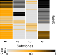
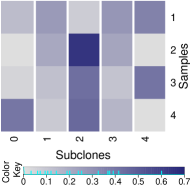
(a) $\bm{Z}_{\text{BC}}^{\text{TRUE}}$	(b) $\hat{\bm{Z}}_{\text{BC}}$	(c) $\hat{\bm{w}}_{\text{BC}}$

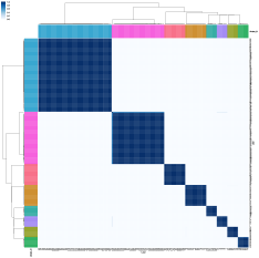
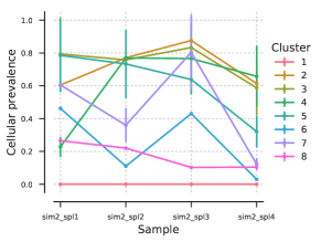
(d) Posterior similarity matrix	(e) Cellular prevalence

Figure A.4: Simulation 2. Posterior inference under BayClone (a, b, c) and PyClone (d, e).

For comparison, we again fit the same simulated data with BayClone and PyClone. BayClone chooses the model with 4 subclones, which still recovers the truth. However, using only SNV data, BayClone can not see the connection between adjacent SNVs, and inference fails to recover $\bm{w}_{\text{BC}}^{\text{TRUE}}$ and therefore $\bm{Z}_{\text{BC}}^{\text{TRUE}}$, even approximately. PyClone infers 8 clusters for the 200 loci, which reasonably recovers the truth. However, since the underlying subclone structure is more complex, the PyClone cellular prevalence is not directly comparable to PairClone outputs.

A.3.3 Simulation 3

In the last simulation we use $T=6$ samples with $C^{\text{TRUE}}=3$ and latent subclones. We still consider $K=100$ mutation pairs. The subclone matrix $\bm{Z}^{\text{TRUE}}$ is shown in Figure A.5(a). For each sample $t$, we generate the subclone proportions from $\bm{w}_{t}^{\text{TRUE}}\sim\mbox{Dir}(0.01,\sigma(14,6,3))$, where $\sigma(14,6,3)$ is a random permutation of $(14,6,3)$. The proportions $\bm{w}^{\text{TRUE}}$ are shown in Figure A.5(b). The parameters $\bm{\rho}^{\text{TRUE}}$ and $N_{tk}$ are generated using the same approach as before, and we use the same $v_{tk2}$ and $v_{tk3}$ as in Simulation 2. Finally, we calculate $\{p_{tkg}^{\text{TRUE}}\}$ and generate read counts $n_{tkg}$ from equation (1) similar to simulation 1.

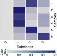
(a) $\bm{Z}^{\text{TRUE}}$	(b) $\bm{w}^{\text{TRUE}}$	(c) $p_{b}(C\mid\bm{n}^{\prime\prime})$
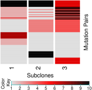
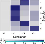
(d) $\hat{\bm{Z}}$	(e) $\hat{\bm{w}}$	(f) Histogram of $(\hat{p}_{tkg}-p_{tkg}^{\text{TRUE}})$

Figure A.5: Simulation 3. Simulation truth $\bm{Z}^{\text{TRUE}}$ and $\bm{w}^{\text{TRUE}}$ (a, b), and posterior inference under PairClone (c, d, e, f).

We fit the model with the same hyperparameter and the same MCMC tuning parameters as in simulation 1. We now use a smaller test sample size, i.e., a smaller fraction $b$ in the transdimensional MCMC. See Section A.5 for a discussion.

Figure A.5(c) shows $p_{b}(C\mid\bm{n}^{\prime\prime})$, with the posterior mode $\hat{C}=3$ recovering the truth. Figures A.5(d, e) show $\hat{\bm{Z}}$ and $\hat{\bm{w}}$. Comparing with panels (a) and (b) we can see an almost perfect recovery of the truth. Figure A.5(f) shows a histogram of the residuals $(\hat{p}_{tkg}-p_{tkg}^{\text{TRUE}})$. The plot indicates a good model fit.

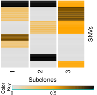
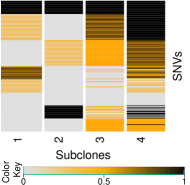
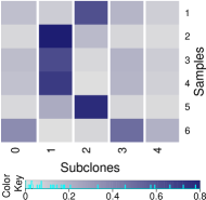
(a) $\bm{Z}_{\text{BC}}^{\text{TRUE}}$	(b) $\hat{\bm{Z}}_{\text{BC}}$	(c) $\hat{\bm{w}}_{\text{BC}}$

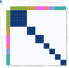
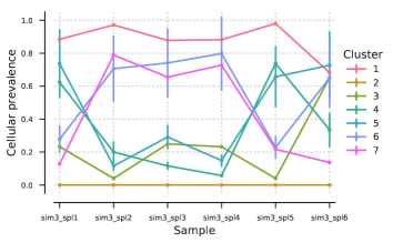
(d) Posterior similarity matrix	(e) Cellular prevalence

Figure A.6: Simulation 3. Posterior inference under BayClone (a, b, c) and PyClone (d, e).

We again compare with inference under BayClone and PyClone. In this case, BayClone chooses the model with 4 subclones, failing to recover the truth. PyClone infers 7 clusters for the 200 loci, which reasonably recovers the truth, but the result is still not directly comparable.

A.4 Simulation with tumor purity incorporated

We report simulation details of the simulation study with tumor purity incorporated in the manuscript (Section 5.2). The simulation setting is the same as simulation 3 in Section A.3.3, except that we substitute the first subclone with a normal subclone. We use exactly the same hyperparameters as those in simulations 2 and 3, and in addition we take $d_{1}^{*}=d_{2}^{*}=1$. Figure A.7 summarizes inference results. Columns in panels (b) and (c) marked with “*” correspond to the normal subclone. Panel (a) shows $p_{b}(C\mid\bm{n}^{\prime\prime})$. Posterior inference recovers the simulation truth, with posterior mode $\hat{C}=2$. Panel (b) shows $\hat{\bm{Z}}$. Comparing with subclones 2 and 3 in Figure A.5(a) we find a good recovery of the simulation truth. Panel (c) shows $\hat{\bm{w}}$, which can be compared with Figure A.5(b).

(a) $p_{b}(C\mid\bm{n}^{\prime\prime})$

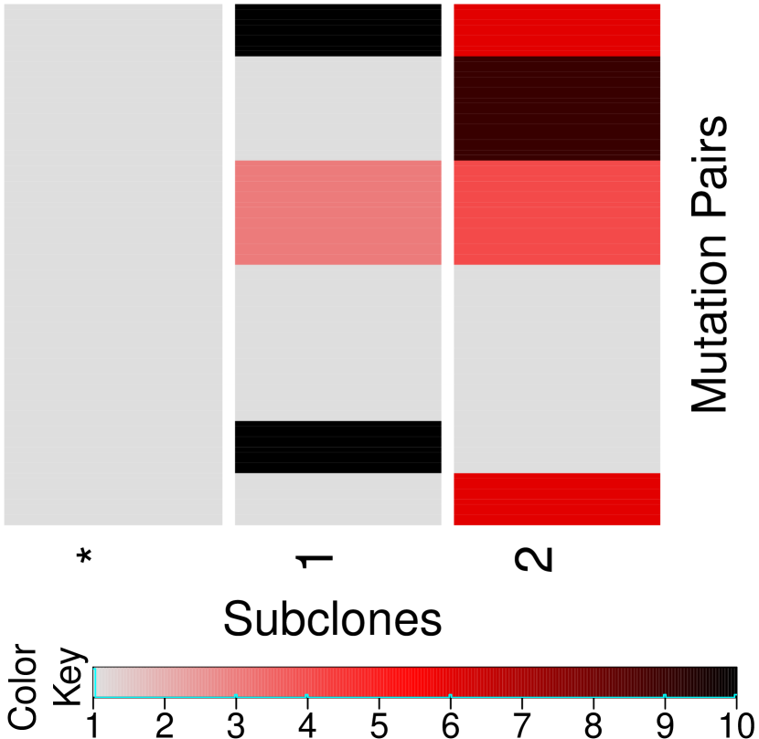
(b) $\hat{\bm{Z}}$

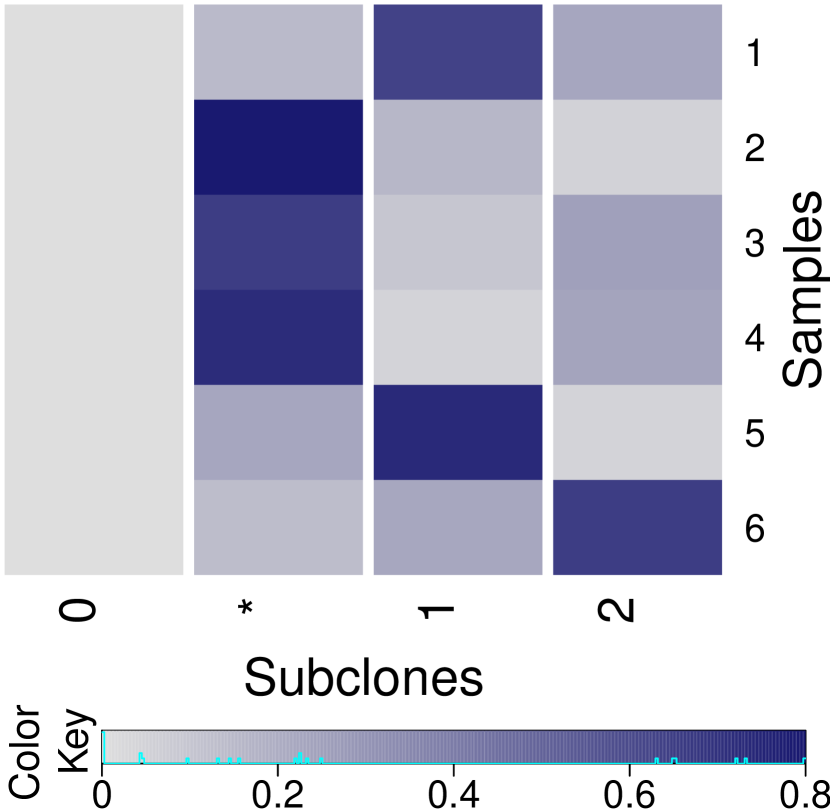
(c) $\hat{\bm{w}}$

Figure A.7: Summary of simulation results with tumor purity incorporated.

A.5 Calibration of $b$

The construction of an informative prior $p_{b}(\bm{x}\mid C)\equiv p(\bm{x}\mid\bm{n}^{\prime},C)$ based on a training sample $\bm{n}^{\prime}$ is similar to the use of a training sample in the construction of the fractional Bayes factor (FBF) of O’Hagan (1995). However, there is an important difference. In the FBF construction the aim is to replace a noninformative prior in the evaluation of a Bayes factor. A minimally informative prior $p_{b}$ with small $b$ suffices. In contrast, here $p_{b}(\bm{x}\mid C)$ is (also) used as proposal distribution in the trans-dimensional MCMC. The aim is to construct a good proposal that fits the data well and thus leads to good acceptance probabilities and a well mixing Markov chain. With the highly informative multinomial likelihood we find that we need a large training sample, that is, large $b$. In Appendix A.2 we show that the effect of using $p_{b}$ is that $p(C\mid\bm{n})$ is approximated by

$$p_{b}(C\mid\bm{n}^{\prime\prime})\propto p(C)p(\bm{n}\mid\bm{u}^{*},C)^{1-b}b^{\;p_{C}/2},$$

where $\bm{u}=\{\bm{\pi},\bm{w},\bm{\rho}\}$ are the parameters other than $\bm{Z}$, $\bm{u}^{*}$ is the maximum likelihood estimate of $\bm{u}$, and $p_{C}$ is the number of unconstrained parameters in $\bm{u}$. Importantly, however, inference on other parameters, $p(\bm{x}\mid C,\bm{n})$, remains entirely unchanged.

Figure A.8: Path plot of $\hat{C}$ with different test sample sizes for three simulations. The true number of subclones are 2, 4, and 3 for simulations 1, 2, and 3, respectively.

We therefore recommend to focus on inference for $C$ when calibrating $b$. Carrying out simulation studies with single and multi-sample data, we find that the simulation truth for $C$ is best recovered with a test sample size $(1-b)\sum_{t=1}^{T}\sum_{k=1}^{K}N_{tk}\approx 160/T$, where $N_{tk}$ is the total number of short reads mapped to mutation pair $k$ in sample $t$. For example, Figure A.8 plots the posterior mode of $C$ against test sample sizes for simulated data in three simulations. For multi-sample data we find (empirically, by simulation) that the test sample size can be reduced, at a rate linear in $T$. In summary we recommend to set $b$ to achieve a test sample size around $160/T$. Following these guidelines, in our implementation in the previous section, we used values $b=0.992$ for simulation 1, $b=0.9998$ for simulation 2, and $b=0.999911$ for simulation 3.

A.6 Lung Cancer Data Analysis Plots

We present two more plots for the lung cancer data analysis (manuscript Section 6). Figure 9(a) shows the posterior distribution $p_{b}(C\mid\bm{n}^{\prime\prime})$ with posterior mode $\hat{C}=2$. Figure 9(b) shows the histogram of realized residuals.

(a) $p_{b}(C\mid\bm{n}^{\prime\prime})$

(b) Histogram of $(\hat{p}_{tkg}-\bar{p}_{tkg})$

Figure A.9: Lung cancer. Posterior inference under PairClone.

A.7 Validation of the MCMC scheme

Validation of the correctness of the sampler.

We first use a scheme to validate the correctness of our MCMC sampler in the style of Geweke (2004). The joint density of the parameters and observed data can be written as $p(\bm{x},\bm{n})=p(\bm{x})p(\bm{n}\mid\bm{x})$. Let $g$ be any function $g:\mathcal{X}\times\mathcal{N}\rightarrow\mathbb{R}$ satisfying $\text{Var}[g(\bm{x},\bm{n})]<\infty$, where $\mathcal{X}$ and $\mathcal{N}$ represent sample spaces of $\bm{x}$ and $\bm{n}$, respectively. Denote by $\bar{g}=E[g(\bm{x},\bm{n})]$, which can be evaluated by independent Monte Carlo simulation from the joint distribution, or in some cases might be known exactly as prior mean of functions of parameters only. Alternatively, the same mean can be estimated by a different Markov chain Monte Carlo scheme for the joint distribution, constructed by an initial draw $\bm{x}^{(0)}\sim p(\bm{x})$, followed by $\bm{n}^{(l)}\sim p(\bm{n}\mid\bm{x}^{(l-1)})$, $\bm{x}^{(l)}\sim q(\bm{x}\mid\bm{x}^{(l-1)},\bm{n}^{(l)})$, and $g^{(l)}=g(\bm{n}^{(l)},\bm{x}^{(l)})$ , for $l=1,\ldots,L$. Under certain conditions, $\{\bm{x}^{(l)},\bm{n}^{(l)}\}$ is ergodic with unique invariant kernel $p(\bm{x},\bm{n})$. If the simulator is error-free, one should have

$$(\bar{g}^{(L)}-\bar{g})/\left[L^{-1}\hat{S}_{g}(0)\right]^{1/2}\xrightarrow{d}N(0,1),$$ (6)

where $\hat{S}_{g}(0)$ is consistent spectral density estimate for $\{g^{(l)},l=1,\ldots,L\}$. In our application, we take $g(\bm{x},\bm{n})=w_{tc}$ and $p_{tkg}$. We set the number of samples $T=4$, and the number of mutation pairs $K=80$. Since our inference on $C$ is not a standard MCMC, we fix $C=3$ here and only consider $\bm{x}=\{\bm{Z},\bm{\pi},\bm{w},\bm{\rho}\}$. Table A.1 shows the statistic (6) for five randomly selected $w_{tc}$ and $p_{tkg}$. The recorded $z$-scores show no evidence for errors in the simulator.

Test statistic	$z$-score	$p$-value
$w_{12}$	-0.4736149	0.6357745
$w_{43}$	-1.441169	0.149537
$p_{1,23,3}$	0.9413715	0.3465145
$p_{3,60,7}$	1.388424	0.1650079
$p_{2,13,2}$	-0.6051894	0.5450532

Table A.1: Geweke’s statistics and the corresponding $z$-scores and $p$-values.

Convergence diagnostic.

Next, we present some convergence diagnostics of our MCMC chain, including trace plots, autocorrelation plots, and test statistics described in Geweke (1991). Those convergence diagnostics are based on the posterior distribution of parameters $p(\bm{x}\mid\bm{n})\propto p(\bm{x})p(\bm{n}\mid\bm{x})$. Let $g$ be any function $g:\mathcal{X}\rightarrow\mathbb{R}$, and $g^{(l)}=g(\bm{x}^{(l)})$ where $\{\bm{x}^{(l)},l=1,\ldots,L\}$ are samples from the posterior. Let

$$\bar{g}^{A}_{L}=L_{A}^{-1}\sum_{l=1}^{L_{A}}g^{(l)},\quad\quad\bar{g}^{B}_{L}=L_{B}^{-1}\sum_{l=l^{*}}^{L}g^{(l)}\;\;\;(l^{*}=L-L_{B}+1),$$

and let $\hat{S}_{g}^{A}(0)$ and $\hat{S}_{g}^{B}(0)$ denote consistent spectral density estimates for $\{g^{(l)},l=1,\ldots,L_{A}\}$ and $\{g^{(l)},l=l^{*},\ldots,L\}$, respectively. If the ratios $L_{A}/L$ and $L_{B}/L$ are fixed, with $(L_{A}+L_{B})/L<1$, then as $L\rightarrow\infty$,

$$(\bar{g}^{A}_{L}-\bar{g}^{B}_{L})/\left[L_{A}^{-1}\hat{S}_{g}^{A}(0)+L_{B}^{-1}\hat{S}_{g}^{B}(0)\right]^{1/2}\xrightarrow{d}N(0,1).$$

In our application, a reasonable choice of $g$ is $g(\bm{x})=p_{tkg}(\bm{Z},\bm{w},\bm{\rho})$. We use simulation 2 as an example, and show some plots and Geweke’s statistics for some randomly chosen $p_{tkg}$. Figure A.10(a, c) shows the trace plot for $p_{tkg}$, with the red dashed line denoting the true value. The posterior samples are centered around the true value and symmetrically distributed. Figure A.10(b, d) shows the autocorrelation plot for $p_{tkg}$. The autocorrelations between MCMC draws are small, indicating good mixing of the chain. Table A.2 shows the Geweke’s statistics for five randomly selected $p_{tkg}$. The $p$-values for them are all greater than 0.05, representing those statistics pass the Geweke’s diagnostic, and there is no strong evidence that the chain does not converge.

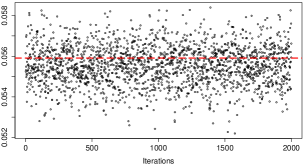
(a) Trace plot of $p_{1,5,2}$	(b) Autocorrelation plot of $p_{1,5,2}$
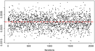
(c) Trace plot of $p_{3,68,7}$	(d) Autocorrelation plot of $p_{3,68,7}$

Figure A.10: Convergence check for Simulation 2.

Test statistic	$z$-score	$p$-value
$p_{1,5,2}$	0.1748906	0.8611656
$p_{3,68,7}$	-0.02609703	0.9791799
$p_{4,25,5}$	0.4454738	0.6559774
$p_{2,96,4}$	-1.341994	0.179598
$p_{1,66,1}$	-0.2727737	0.7850272

Table A.2: Convergence check for Simulation 2.

References

- Almendro et al. (2013) Almendro, V., A. Marusyk, and K. Polyak (2013). Cellular heterogeneity and molecular evolution in cancer. Annual Review of Pathology: Mechanisms of Disease 8, 277–302.
- Broderick et al. (2013) Broderick, T., J. Pitman, M. I. Jordan, et al. (2013). Feature allocations, probability functions, and paintboxes. Bayesian Analysis 8(4), 801–836.
- Brooks et al. (2011) Brooks, S., A. Gelman, G. Jones, and X.-L. Meng (2011). Handbook of Markov Chain Monte Carlo. CRC Press.
- Carter et al. (2012) Carter, S. L., K. Cibulskis, E. Helman, A. McKenna, H. Shen, T. Zack, P. W. Laird, R. C. Onofrio, W. Winckler, B. A. Weir, et al. (2012). Absolute quantification of somatic DNA alterations in human cancer. Nature biotechnology 30(5), 413–421.
- Church et al. (2011) Church, D. M., V. A. Schneider, T. Graves, K. Auger, F. Cunningham, N. Bouk, H.-C. Chen, R. Agarwala, W. M. McLaren, G. R. Ritchie, et al. (2011). Modernizing reference genome assemblies. PLoS Biol 9(7), e1001091.
- Deshwar et al. (2015) Deshwar, A. G., S. Vembu, C. K. Yung, G. H. Jang, L. Stein, and Q. Morris (2015). Phylowgs: Reconstructing subclonal composition and evolution from whole-genome sequencing of tumors. Genome Biology 16(1), 35.
- Dexter et al. (1978) Dexter, D. L., H. M. Kowalski, B. A. Blazar, Z. Fligiel, R. Vogel, and G. H. Heppner (1978). Heterogeneity of tumor cells from a single mouse mammary tumor. Cancer Research 38(10), 3174–3181.
- Gelfand and Dey (1994) Gelfand, A. E. and D. K. Dey (1994). Bayesian model choice: asymptotics and exact calculations. Journal of the Royal Statistical Society. Series B (Methodological), 501–514.
- Geweke (1991) Geweke, J. (1991). Evaluating the accuracy of sampling-based approaches to the calculation of posterior moments, Volume 196. Federal Reserve Bank of Minneapolis, Research Department Minneapolis, MN, USA.
- Geweke (2004) Geweke, J. (2004). Getting it right: Joint distribution tests of posterior simulators. Journal of the American Statistical Association 99(467), 799–804.
- Geyer (1991) Geyer, C. J. (1991). Markov chain monte carlo maximum likelihood.
- Green (1995) Green, P. J. (1995). Reversible jump Markov chain Monte Carlo computation and Bayesian model determination. Biometrika 82(4), 711 – 732.
- Griffiths and Ghahramani (2011) Griffiths, T. L. and Z. Ghahramani (2011). The Indian buffet process: An introduction and review. Journal of Machine Learning Research 12, 1185–1224.
- Jiao et al. (2014) Jiao, W., S. Vembu, A. G. Deshwar, L. Stein, and Q. Morris (2014). Inferring clonal evolution of tumors from single nucleotide somatic mutations. BMC bioinformatics 15(1), 35.
- Kim et al. (2012) Kim, Y., L. James, and R. Weissbach (2012). Bayesian analysis of multistate event history data: beta-Dirichlet process prior. Biometrika 99(1), 127–140.
- Lee et al. (2016) Lee, J., P. Mueller, S. Sengupta, K. Gulukota, and Y. Ji (2016). Bayesian inference for intratumour heterogeneity in mutations and copy number variation. Journal of the Royal Statistical Society: Series C 65(4), 547–563.
- Lee et al. (2015) Lee, J., P. Müller, K. Gulukota, Y. Ji, et al. (2015). A Bayesian feature allocation model for tumor heterogeneity. The Annals of Applied Statistics 9(2), 621–639.
- Li (2014) Li, H. (2014). Toward better understanding of artifacts in variant calling from high-coverage samples. Bioinformatics 30(20), 2843–2851.
- Li and Durbin (2009) Li, H. and R. Durbin (2009). Fast and accurate short read alignment with Burrows–Wheeler transform. Bioinformatics 25(14), 1754–1760.
- Liu (2008) Liu, J. S. (2008). Monte Carlo strategies in scientific computing. Springer Science & Business Media.
- Mardis (2008) Mardis, E. R. (2008). Next-generation DNA sequencing methods. Annu. Rev. Genomics Hum. Genet. 9, 387–402.
- Marjanovic et al. (2013) Marjanovic, N. D., R. A. Weinberg, and C. L. Chaffer (2013). Cell plasticity and heterogeneity in cancer. Clinical Chemistry 59(1), 168–179.
- McKenna et al. (2010) McKenna, A., M. Hanna, E. Banks, A. Sivachenko, K. Cibulskis, A. Kernytsky, K. Garimella, D. Altshuler, S. Gabriel, M. Daly, et al. (2010). The Genome Analysis Toolkit: a MapReduce framework for analyzing next-generation DNA sequencing data. Genome Research 20(9), 1297–1303.
- Miller et al. (2014) Miller, C. A., B. S. White, N. D. Dees, M. Griffith, J. S. Welch, O. L. Griffith, R. Vij, M. H. Tomasson, T. A. Graubert, M. J. Walter, et al. (2014). Sciclone: Inferring clonal architecture and tracking the spatial and temporal patterns of tumor evolution. PLoS Computational Biology 10(8), e1003665.
- Nik-Zainal et al. (2012) Nik-Zainal, S., L. B. Alexandrov, D. C. Wedge, P. Van Loo, C. D. Greenman, K. Raine, D. Jones, J. Hinton, J. Marshall, L. A. Stebbings, et al. (2012). Mutational processes molding the genomes of 21 breast cancers. Cell 149(5), 979–993.
- Oesper et al. (2013) Oesper, L., A. Mahmoody, and B. J. Raphael (2013). Theta: inferring intra-tumor heterogeneity from high-throughput DNA sequencing data. Genome Biol 14(7), R80.
- O’Hagan (1995) O’Hagan, A. (1995). Fractional Bayes factor for model comparison. Journal of the Royal Statistical Society. Series B (Methodological) 57(1), 99 – 138.
- Parmigiani et al. (2002) Parmigiani, G., E. S. Garrett, R. Anbazhagan, and E. Gabrielson (2002). A statistical framework for expression-based molecular classification in cancer. Journal of the Royal Statistical Society: Series B (Statistical Methodology) 64(4), 717–736.
- Polyak (2011) Polyak, K. (2011). Heterogeneity in breast cancer. The Journal of Clinical Investigation 121(10), 3786.
- Roth et al. (2014) Roth, A., J. Khattra, D. Yap, A. Wan, E. Laks, J. Biele, G. Ha, S. Aparicio, A. Bouchard-Côté, and S. P. Shah (2014). PyClone: statistical inference of clonal population structure in cancer. Nature methods 11(4), 396–398.
- Sengupta et al. (2015) Sengupta, S., K. Gulukota, Y. Zhu, C. Ober, K. Naughton, W. Wentworth-Sheilds, and Y. Ji (2015). Ultra-fast local-haplotype variant calling using paired-end DNA-sequencing data reveals somatic mosaicism in tumor and normal blood samples. Nucleic Acids Research (to appear).
- Sengupta et al. (2013) Sengupta, S., J. Ho, and A. Banerjee (2013). Two models involving Bayesian nonparametric techniques. Technical report, University of Florida.
- Sengupta et al. (2015) Sengupta, S., J. Wang, J. Lee, P. Müller, K. Gulukota, A. Banerjee, and Y. Ji (2015). Bayclone: Bayesian nonparametric inference of tumor subclones using NGS data. Pacific Symposium of Biocomputing, 467–478.
- Shackleton et al. (2009) Shackleton, M., E. Quintana, E. R. Fearon, and S. J. Morrison (2009). Heterogeneity in cancer: cancer stem cells versus clonal evolution. Cell 138(5), 822–829.
- Stingl and Caldas (2007) Stingl, J. and C. Caldas (2007). Molecular heterogeneity of breast carcinomas and the cancer stem cell hypothesis. Nature Reviews Cancer 7(10), 791–799.
- Strino et al. (2013) Strino, F., F. Parisi, M. Micsinai, and Y. Kluger (2013). Trap: a tree approach for fingerprinting subclonal tumor composition. Nucleic acids research 41(17), e165–e165.
- Van Loo et al. (2010) Van Loo, P., S. H. Nordgard, O. C. Lingjærde, H. G. Russnes, I. H. Rye, W. Sun, V. J. Weigman, P. Marynen, A. Zetterberg, B. Naume, et al. (2010). Allele-specific copy number analysis of tumors. Proceedings of the National Academy of Sciences 107(39), 16910–16915.
- Zare et al. (2014) Zare, H., J. Wang, A. Hu, K. Weber, J. Smith, D. Nickerson, C. Song, D. Witten, C. A. Blau, and W. S. Noble (2014). Inferring clonal composition from multiple sections of a breast cancer. PLoS Computational Biology 10(7), e1003703.