Sequence Modeling via Segmentations

Abstract

Segmental structure is a common pattern in many types of sequences such as phrases in human languages. In this paper, we present a probabilistic model for sequences via their segmentations. The probability of a segmented sequence is calculated as the product of the probabilities of all its segments, where each segment is modeled using existing tools such as recurrent neural networks. Since the segmentation of a sequence is usually unknown in advance, we sum over all valid segmentations to obtain the final probability for the sequence. An efficient dynamic programming algorithm is developed for forward and backward computations without resorting to any approximation. We demonstrate our approach on text segmentation and speech recognition tasks. In addition to quantitative results, we also show that our approach can discover meaningful segments in their respective application contexts.

1 Introduction

Segmental structure is a common pattern in many types of sequences, typically, phrases in human languages and letter combinations in phonotactics rules. For instances,

• Phrase structure. “Machine learning is part of artificial intelligence” $\rightarrow$ [Machine learning] [is] [part of] [artificial intelligence].

• Phonotactics rules. “thought” $\rightarrow$ [th][ou][ght].

The words or letters in brackets “[ ]” are usually considered as meaningful segments for the original sequences. In this paper, we hope to incorporate this type of segmental structure information into sequence modeling.

Mathematically, we are interested in constructing a conditional probability distribution $p(y|x)$, where output $y$ is a sequence and input $x$ may or may not be a sequence. Suppose we have a segmented sequence. Then the probability of this sequence is calculated as the product of the probabilities of its segments, each of which is modeled using existing tools such as recurrent neural networks (RNNs), long-short term memory (LSTM) (Hochreiter & Schmidhuber, 1997), or gated recurrent units (GRU) (Chung et al., 2014). When the segmentation for a sequence is unknown, we sum over the probabilities from all valid segmentations. In the case that the input is also a sequence, we further need to sum over all feasible alignments between inputs and output segmentations. This sounds complicated. Fortunately, we show that both forward and backward computations can be tackled with a dynamic programming algorithm without resorting to any approximations.

This paper is organized as follows. In Section 2, we describe our mathematical model which constructs the probability distribution of a sequence via its segments, and discuss related work. In Section 3, we present an efficient dynamic programming algorithm for forward and backward computations, and a beam search algorithm for decoding the output. Section 4 includes two case studies to demonstrate the usefulness of our approach through both quantitative and qualitative results. We conclude this paper and discuss future work in Section 5.

2 Sequence modeling via segmentations

In this section, we present our formulation of sequence modeling via segmentations. In our model, the output is always a sequence, while the input may or may not be a sequence. We first consider the non-sequence input case, and then move to the sequence input case. We then show how to carry over information across segments when needed. Related work is also discussed here.

2.1 Case I: Mapping from non-sequence to sequence

Figure 1: For Section 2.1. Given output $y_{1:3}$ and its segmentation $a_{1}=\{y_{1},\$\}$ and $a_{2}=\{y_{2},y_{3},\$\}$, input $x$ controls the initial states of both segments. Note that $\pi(a_{1:t-1})$ is omitted here.

Assume the input $x$ is a fixed-length vector. Let the output sequence be $y_{1:T}$. We are interested in modeling the probability $p(y_{1:T}|x)$ via the segmentations of $y_{1:T}$. Denote by $\mathcal{S}_{y}$ the set containing all valid segmentations of $y_{1:T}$. Then for any segmentation $a_{1:\tau_{a}}\in\mathcal{S}_{y}$, we have $\pi(a_{1:\tau_{a}})=y_{1:T}$, where $\pi(\cdot)$ is the concatenation operator and $\tau_{a}$ is the number of segments in this segmentation. For example, let $T=5$ and $\tau_{a}=3.$ Then one possible $a_{1:\tau_{a}}$ could be like $a_{1:\tau_{a}}=\{\{y_{1},\$\},\{y_{2},y_{3},\$\},\{y_{4},y_{5},\$\}\}$, where $\$$ denotes the end of a segment. Note that symbol $\$$ will be ignored in the concatenation operator $\pi(\cdot)$. Empty segments, those containing only $\$$, are not permitted in our setting. Note that while the number of distinct segments for a length-$T$ sequence is $O(T^{2})$, the number of distinct segmentations, that is, $|\mathcal{S}_{y}|$, is exponentially large.

Since the segmentation is unknown in advance, the probability of the sequence $y_{1:T}$ is defined as the sum of the probabilities from all the segmentations in $\mathcal{S}_{y}$,

$$p(y_{1:T}|x) \triangleq\sum_{a_{1:\tau_{a}}\in\mathcal{S}_{y}}p(a_{1:\tau_{a}}|x)$$

$$=\sum_{a_{1:\tau_{a}}\in\mathcal{S}_{y}}\prod_{t=1}^{\tau_{a}}p(a_{t}|x,\pi(a_{1:t-1})),$$ (1)

where $p(a_{1:\tau_{a}}|x)$ is the probability for segmentation $a_{1:\tau_{a}}$ given input $x$, and $p(a_{t}|x,\pi(a_{1:t-1}))$ is the probability for segment $a_{t}$ given input $x$ and the concatenation of all previous segments $\pi(a_{1:t-1})$. Figure 1 illustrates a possible relationship between $x$ and $y_{1:T}$ given one particular segmentation. We choose to model the segment probability $p(a_{t}|x,\pi(a_{1:t-1}))$ using recurrent neural networks (RNNs), such as LSTM or GRU, with a softmax probability function. Input $x$ and concatenation $\pi(a_{1:t-1})$ determine the initial state for this RNN. (All segments’ RNNs share the same network parameters.) However, since $|\mathcal{S}_{y}|$ is exponentially large, Eq. 1 cannot be directly computed. We defer the computational details to Section 3.

2.2 Case II: Mapping from sequence to sequence

Now we assume the input is also a sequence $x_{1:T^{\prime}}$ and the output remains as $y_{1:T}$. We make a monotonic alignment assumption—each input element $x_{t}$ emits one segment $a_{t}$, which is then concatenated as $\pi(a_{1:T^{\prime}})$ to obtain $y_{1:T}$. Different from the case when the input is not a sequence, we allow empty segments in the emission, i.e., $a_{t}=\{\$\}$ for some $t$, such that any segmentation of $y_{1:T}$ will always consist of exactly $T^{\prime}$ segments with possibly some empty ones. In other words, all valid segmentations for the output is in set $\mathcal{S}_{y}\triangleq\{a_{1:T^{\prime}}:\pi(a_{1:T^{\prime}})=y_{1:T}\}$. Since an input element can choose to emit an empty segment, we name this particular method as “Sleep-WAke Networks” (SWAN). See Figure 2 for an example of the emitted segmentation of $y_{1:T}$.

Again, as in Eq. 1, the probability of the sequence $y_{1:T}$ is defined as the sum of the probabilities of all the segmentations in $\mathcal{S}_{y}$,

$$p(y_{1:T}|x_{1:T^{\prime}})\triangleq\sum_{a_{1:T^{\prime}}\in S_{y}}\prod_{t=1}^{T^{\prime}}p(a_{t}|x_{t},\pi(a_{1:t-1})),$$ (2)

where $p(a_{t}|x_{t},\pi(a_{1:t-1}))$ is the probability of segment $a_{t}$ given input element $x_{t}$ and the concatenation of all previous segments $\pi(a_{1:t-1})$. In other words, input element $x_{t}$ emits segment $a_{t}$. Again this segment probability can be modeled using an RNN with a softmax probability function with $x_{t}$ and $\pi(a_{1:t-1})$ providing the information for the initial state. The number of possible segments for $y_{1:T}$ is $O(T^{\prime}T^{2})$. Similar to Eq. 1, a direct computation of Eq. 2 is not feasible since $|\mathcal{S}_{y}|$ is exponentially large. We address the computational details in Section 3.

Figure 2: For Section 2.2. SWAN emits one particular segmentation of $y_{1:T}$ with $x_{1}$ waking (emits $y_{1}$) and $x_{4}$ waking (emits $y_{2}$ and $y_{3}$) while $x_{2}$, $x_{3}$ and $x_{5}$ sleeping. SWAN needs to consider all valid segmentations like this for $y_{1:T}$.

2.3 Carrying over information across segments

Figure 3: For Section 2.3. SWAN carries over information across segments using a separate RNN. Here the segments are $a_{t-2}=\{y_{j-1},\$\}$, $a_{t-1}=\{\$\}$ and $a_{t}=\{y_{j},y_{j+1},\$\}$ emitted by input elements $x_{t-2}$, $x_{t-1}$ and $x_{t}$ respectively.

Note that we do not assume that the segments in a segmentation are conditionally independent. Take Eq. 2 as an example, the probability of a segment $a_{t}$ given $x_{t}$ is defined as $p(a_{t}|x_{t},\pi(a_{1:t-1}))$, which also depends on the concatenation of all previous segments $\pi(a_{1:t-1})$. We take an approach inspired by the sequence transducer (Graves, 2012) to use a separate RNN to model $\pi(a_{1:t-1})$. The hidden state of this RNN and input $x_{t}$ are used as the initial state of the RNN for segment $a_{t}$. (We simply add them together in our speech recognition experiment.) This allows all previous emitted outputs to affect this segment $a_{t}$. Figure 3 illustrates this idea. The significance of this approach is that it still permits the exact dynamic programming algorithm as we will describe in Section 3.

2.4 Related work

Our approach, especially SWAN, is inspired by connectionist temporal classification (CTC) (Graves et al., 2006) and the sequence transducer (Graves, 2012). CTC defines a distribution over the output sequence that is not longer than the input sequence. To appropriate map the input to the output, CTC marginalizes out all possible alignments using dynamic programming. Since CTC does not model the interdependencies among the output sequence, the sequence transducer introduces a separate RNN as a prediction network to bring in output-output dependency, where the prediction network works like a language model.

SWAN can be regarded as a generalization of CTC to allow segmented outputs. Neither CTC nor the sequence transducer takes into account segmental structures of output sequences. Instead, our method constructs a probabilistic distribution over output sequences by marginalizing all valid segmentations. This introduces additional nontrivial computational challenges beyond CTC and the sequence transducer. When the input is also a sequence, our method then marginalizes the alignments between the input and the output segmentations. Since outputs are modeled with segmental structures, our method can be applied to the scenarios where the input is not a sequence or the input length is shorter than the output length, while CTC cannot. When we need to carry information across segments, we borrow the idea of the sequence transducer to use a separate RNN. Although it is suspected that using a separate RNN could result in a loosely-coupled model (Graves, 2013; Jaitly et al., 2016) that might hinder the performance, we do not find it to be an issue in our approach. This is perhaps due to our use of the output segmentation—the hidden states of the separate RNN are not directly used for prediction but as the initial states of the RNN for the segments, which strengthens their dependencies on each other.

SWAN itself is most similar to the recent work on the neural transducer (Jaitly et al., 2016), although we start with a different motivation. The motivation of the neural transducer is to allow incremental predictions as input streamingly arrives, for example in speech recognition. From the modeling perspective, it also assumes that the output is decomposed into several segments and the alignments are unknown in advance. However, its assumption that hidden states are carried over across the segments prohibits exact marginalizing all valid segmentations and alignments. So they resorted to find an approximate “best” alignment with a dynamic programming-like algorithm during training or they might need a separate GMM-HMM model to generate alignments in advance to achieve better results. Otherwise, without carrying information across segments results in sub-optimal performance as shown in Jaitly et al. (2016). In contrast, our method of connecting the segments described in Section 2.3 preserves the advantage of exact marginalization over all possible segmentations and alignments while still allowing the previous emitted outputs to affect the states of subsequent segments. This allows us to obtain a comparable good performance without using an additional alignment tool.

Another closely related work is the online segment to segment neural transduction (Yu et al., 2016). This work treats the alignments between the input and output sequences as latent variables and seeks to marginalize them out. From this perspective, SWAN is similar to theirs. However, our work explicitly takes into account output segmentations, extending the scope of its application to the case when the input is not a sequence. Our work is also related to semi-Markov conditional random fields (Sarawagi & Cohen, 2004), segmental recurrent neural networks (Kong et al., 2015) and segmental hidden dynamic model (Deng & Jaitly, 2015), where the segmentation is applied to the input sequence instead of the output sequence.

3 Forward, backward and decoding

In this section, we first present the details of forward and backward computations using dynamic programming. We then describe the beam search decoding algorithm. With these algorithms, our approach becomes a standalone loss function that can be used in many applications. Here we focus on developing the algorithm for the case when the input is a sequence. When the input is not a sequence, the corresponding algorithms can be similarly derived.

3.1 Forward and backward propagations

Forward.

Consider calculating the result for Eq. 2. We first define the forward and backward probabilities,

$$\alpha_{t}(j) =p(y_{1:j}|x_{1:t}),$$

$$\beta_{t}(j) =p(y_{j+1:T}|x_{t+1:T^{\prime}},y_{1:j}),$$

where forward $\alpha_{t}(j)$ represents the probability that input $x_{1:t}$ emits output $y_{1:j}$ and backward $\beta_{t}(j)$ represents the probability that input $x_{t+1:T^{\prime}}$ emits output $y_{j+1:T}$. Using $\alpha_{t}(j)$ and $\beta_{t}(j)$, we can verify the following, for any $t=0,1,...,T^{\prime}$,

$$p(y_{1:T}|x_{1:T^{\prime}})=\sum_{j=0}^{T}\alpha_{t}(j)\beta_{t}(j),$$ (3)

where the summation of $j$ from $0$ to $T$ is to enumerate all possible two-way partitions of output $y_{1:T}$. A special case is that $p(y_{1:T}|x_{1:T^{\prime}})=\alpha_{T^{\prime}}(T)=\beta_{0}(0)$. Furthermore, we have following dynamic programming recursions according to the property of the segmentations,

$$\alpha_{t}(j) =\sum_{j^{\prime}=0}^{j}\alpha_{t-1}(j^{\prime})p(y_{j^{\prime}+1:j}|x_{t}),$$ (4)

$$\beta_{t}(j) =\sum_{j^{\prime}=j}^{T}\beta_{t+1}(j^{\prime})p(y_{j+1:j^{\prime}}|x_{t+1}),$$ (5)

where $p(y_{j^{\prime}+1:j}|x_{t})$ is the probability of the segment $y_{j^{\prime}+1:j}$ emitted by $x_{t}$ and $p(y_{j+1:j^{\prime}}|x_{t+1})$ is similarly defined. When $j=j^{\prime}$, notation $y_{j+1:j^{\prime}}$ indicates an empty segment with previous output as $y_{1:j}$. For simplicity, we omit the notation for those previous outputs, since it does not affect the dynamic programming algorithm. As we discussed before, $p(y_{j^{\prime}+1:j}|x_{t})$ is modeled using an RNN with a softmax probability function. Given initial conditions $\alpha_{0}(0)=1$ and $\beta_{T^{\prime}}(T)=1$, we can efficiently compute the probability of the entire output $p(y_{1:T}|x_{1:T^{\prime}})$.

Backward.

We only show how to compute the gradient w.r.t $x_{t}$ since others can be similarly derived. Given the representation of $p(y_{1:T}|x_{1:T^{\prime}})$ in Eq. 3 and the dynamic programming recursion in Eq. 4, we have

$$\frac{\partial\log p(y_{1:T}|x_{1:T^{\prime}})}{\partial x_{t}}=\sum_{j^{\prime}=0}^{T}\sum_{j=0}^{j^{\prime}}w_{t}(j,j^{\prime})\frac{\partial\log p(y_{j+1:j^{\prime}}|x_{t})}{\partial x_{t}},$$ (6)

where $w_{t}(j,j^{\prime})$ is defined as

$$w_{t}(j,j^{\prime})\triangleq{\alpha_{t-1}(j)\beta_{t}(j^{\prime})}\frac{p(y_{j+1:j^{\prime}}|x_{t})}{p(y_{1:T}|x_{1:T^{\prime}})}.$$ (7)

Thus, the gradient w.r.t. $x_{t}$ is a weighted linear combination of the contributions from related segments.

More efficient computation for segment probabilities.

The forward and backward algorithms above assume that all segment probabilities, $\log p(y_{j+1:j^{\prime}}|x_{t})$ as well as their gradients $\frac{\partial\log p(y_{j+1:j^{\prime}}|x_{t})}{\partial x_{t}}$, for $0\leq j\leq j^{\prime}\leq T$ and $0\leq t\leq T^{\prime}$, are already computed. There are $O(T^{\prime}T^{2})$ of such segments. And if we consider each recurrent step as a unit of computation, we have the computational complexity as $O(T^{\prime}T^{3})$. Simply enumerating everything, although parallelizable for different segments, is still expensive.

We employ two additional strategies to allow more efficient computations. The first is to limit the maximum segment length to be $L$, which reduces the computational complexity to $O(T^{\prime}TL^{2})$. The second is to explore the structure of the segments to further reduce the complexity to $O(T^{\prime}TL)$. This is an important improvement, without which we find the training would be extremely slow.

The key observation for the second strategy is that the computation for the longest segment can be used to cover those for the shorter ones. First consider forward propagation with $j$ and $t$ fixed. Suppose we want to compute $\log p(y_{j+1:j^{\prime}}|x_{t})$ for any $j^{\prime}=j,...,j+L$, which contains $L+1$ segments, with the length ranging from $0$ to $L$. In order to compute for the longest segment $\log p(y_{j+1:j+L}|x_{t})$, we need the probabilities for $p(y=y_{j+1}|x_{t},h_{0})$, $p(y=y_{j+2}|y_{j+1},x_{t},h_{1})$, …, $p(y=y_{j+L}|y_{j+L-1},x_{t},h_{L-1})$ and $p(y=\$|y_{j+L},x_{t},h_{L})$, where $h_{l}$, $l=0,1,...,L$, are the recurrent states. Note that this process also gives us the probability distributions needed for the shorter segments when $j^{\prime}=j,...,j+L-1$. For backward propagation, we observe that, from Eq. 6, each segment has its own weight on the contribution to the gradient, which is $w_{t}(j,j^{\prime})$ for $p(y_{j+1:j^{\prime}}|x_{t})$, $j^{\prime}=j,...,j+L$. Thus all we need is to assign proper weights to the corresponding gradient entries for the longest segment $y_{j+1:j+L}$ in order to integrate the contributions from the shorter ones. Figure 4 illustrates the forward and backward procedure.

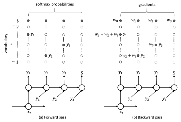
Figure 4: Illustration for an efficient computation for segments $y_{j+1:j^{\prime}}$, $j^{\prime}=j,j+1,...,j+L$ with one pass on the longest segment $y_{j+1:j+L}$, where $V$ is the vocabulary size and $\$$ is the symbol for the end of a segment. In this example, we use $j=0$ and $L=3$. Thus we have four possible segments $\{\$\}$, $\{y_{1},\$\}$, $\{y_{1},y_{2},\$\}$ and $\{y_{1},y_{2},y_{3},\$\}$ given input $x_{t}$. (a) Forward pass. Shaded small circles indicate the softmax probabilities needed to compute the probabilities of all four segments. (b) Backward pass. The weights are $w_{j^{\prime}}\triangleq w_{t}(0,j^{\prime})$ defined in Eq.7 for $j^{\prime}=0,1,2,3$ for four segments mentioned above. Shaded small circles are annotated with the gradient values while unshaded ones have zero gradients. For example, $y_{1}$ has a gradient of $w_{1}+w_{2}+w_{3}$ since $y_{1}$ appears in three segment $\{y_{1},\$\}$, $\{y_{1},y_{2},\$\}$ and $\{y_{1},y_{2},y_{3},\$\}$.

3.2 Beam search decoding

Although it is possible compute the output sequence probability using dynamic programming during training, it is impossible to do a similar thing during decoding since the output is unknown. We thus resort to beam search. The beam search for SWAN is more complex than the simple left-to-right beam search algorithm used in standard sequence-to-sequence models (Sutskever et al., 2014). In fact, for each input element $x_{t}$, we are doing a simple left-to-right beam search decoder. In addition, different segmentations might imply the same output sequence and we need to incorporate this information into beam search as well. To achieve this, each time after we process an input element $x_{t}$, we merge the partial candidates with different segments into one candidate if they indicate the same partial sequence. This is reasonable because the emission of the next input element $x_{t+1}$ only depends on the concatenation of all previous segments as discussed in Section 2.3. Algorithm 1 shows the details of the beam search decoding algorithm.

Algorithm 1 SWAN beam search decoding

  Input: input $x_{1:T^{\prime}}$, beam size $B$, maximum segment length $L$, $\mathcal{Y}=\{\varnothing\}$ and $\mathcal{P}=\{\varnothing:1\}$.

  for $t=1$ to $T^{\prime}$ do

    // A left-to-right beam search given $x_{t}$.

    Set local beam size $b=B$, $\mathcal{Y}_{t}=\{\}$ and $\mathcal{P}_{t}=\{\}$.

    for $j=0$ to $L$ do

       for ${\bf y}\in\mathcal{Y}$ do

          Compute the distribution of the next output for current segment, $p(y_{j}|{\bf y},x_{t})$.

       end for

       if $j=L$ then

          // Reaching the maximum segment length.

          for ${\bf y}\in\mathcal{Y}$ do

             $\mathcal{P}({\bf y})\leftarrow\mathcal{P}({\bf y})p(y_{j}=\$|{\bf y},x_{t})$

          end for

          Choose $b$ candidates with highest probabilities $\mathcal{P}({\bf y})$ from $\mathcal{Y}$ and move them into $\mathcal{Y}_{t}$ and $\mathcal{P}_{t}$.

       else

          Choose a set $\mathcal{Y}_{\rm tmp}$ containing $b$ candidates with highest probabilities $\mathcal{P}({\bf y})p(y_{j}|{\bf y},x_{t})$ out of all pairs $\{{\bf y},y_{j}\}$, where ${\bf y}\in\mathcal{Y}$ and $y_{i}\in\{1,...,V,\$\}$.

          for $\{{\bf y},y_{j}\}\in\mathcal{Y}_{\rm tmp}$ do

             $\mathcal{P}({\bf y})\leftarrow\mathcal{P}({\bf y})p(y_{j}|{\bf y},x_{t})$.

             if $y_{j}=\$$ then

               Move ${\bf y}$ from $\mathcal{Y}$ and $\mathcal{P}$ into $\mathcal{Y}_{t}$ and $\mathcal{P}_{t}$.

               $b\leftarrow b-1$.

             else

               ${\bf y}\leftarrow\{{\bf y},y_{j}\}$

             end if

          end for

       end if

       if $b=0$ then

          break

       end if

    end for

    Update $\mathcal{Y}\leftarrow\mathcal{Y}_{t}$ and $\mathcal{P}\leftarrow\mathcal{P}_{t}$.

    // Merge duplicate candidates in ${\mathcal{Y}}$.

    while There exists ${\bf y}_{i}={\bf y}_{i^{\prime}}$ for any ${\bf y}_{i},{\bf y}_{i^{\prime}}\in\mathcal{Y}$ do

       $\mathcal{P}({\bf y}_{i})\leftarrow\mathcal{P}({\bf y}_{i})+\mathcal{P}({\bf y}_{i^{\prime}})$

       Remove ${\bf y}_{i^{\prime}}$ from ${\mathcal{Y}}$ and ${\mathcal{P}}$.

    end while

  end for

  Return: output ${\bf y}$ with the highest probability from $\mathcal{Y}$.

4 Experiments

In this section, we apply our method to two applications, one unsupervised and the other supervised. These include 1) content-based text segmentation, where the input to our distribution is a vector (constructed using a variational autoencoder for text) and 2) speech recognition, where the input to our distribution is a sequence (of acoustic features).

4.1 Content-based text segmentation

This text segmentation task corresponds to an application of a simplified version of the non-sequence-input model in Section 2.1, where we drop the term $\pi(a_{1:t-1})$ in Eq.1.

Model description.

In this task, we would like to automatically discover segmentations for textual content. To this end, we build a simple model inspired by latent Dirichlet allocation (LDA) (Blei et al., 2003) and neural variational inference for texts (Miao et al., 2016).

LDA assumes that the words are exchangeable within a document—“bag of words” (BoW). We generalize this assumption to the segments within each segmentation—“bag of segments”. In other words, if we had a pre-segmented document, all segments would be exchangeable. However, since we do not have a pre-segmented document, we assume that for any valid segmentation. In addition, we choose to drop the term $\pi(a_{1:t-1})$ in Eq.1 in our sequence distribution so that we do not carry over information across segments. Otherwise, the segments are not exchangeable. This is designed to be comparable with the exchangeability assumption in LDA, although we can definitely use the carry-over technique in other occasions.

Similar to LDA, for a document with words $y_{1:T}$, we assume that a topic-proportion like vector, $\theta$, controls the distribution of the words. In more details, we define $\theta(\zeta)\propto\exp(\zeta)$, where $\zeta\sim\mathcal{N}(0,I)$. Then the log likelihood of words $y_{1:T}$ is defined as

$$\log p(y_{1:T}) =\log\mathbb{E}_{p(\zeta)}[p(y_{1:T}|W\theta(\zeta))]$$

$$\textstyle\geq\mathbb{E}_{q(\zeta)}[\log p(y_{1:T}|W\theta(\zeta))]+\mathbb{E}_{q(\zeta)}\left[\log\frac{p(\zeta)}{q(\zeta)}\right],$$

where the last inequality follows the variational inference principle (Jordan, 1999) with variational distribution $q(\zeta)$. Here $p(y_{1:T}|W\theta(\zeta))$ is modeled as Eq.1 with $W\theta(\zeta)$ as the input vector “$x$” and $W$ being another weight matrix. Note again that $\pi(a_{1:t-1})$ is not used in $p(y_{1:T}|W\theta(\zeta))$.

For variational distribution $q(\zeta)$, we use variational autoencoder to model it as an inference network (Kingma & Welling, 2013; Rezende et al., 2014). We use the form similar to Miao et al. (2016), where the inference network is a feed-forward neural network and its input is the BoW of the document — $q(\zeta)\triangleq q(\zeta|{\rm BoW}(y_{1:T}))$.

Predictive likelihood comparison with LDA.

We use two datasets including AP (Associated Press, $2,246$ documents) from Blei et al. (2003) and CiteULike scientific article abstracts ($16,980$ documents) from Wang & Blei (2011). Stop words are removed and a vocabulary size of $10,000$ is chosen by tf-idf for both datasets. Punctuations and stop words are considered to be known segment boundaries for this experiment. For LDA, we use the variational EM implementation taken from authors’ website.

We vary the number of topics to be $100$, $150$, $200$, $250$ and $300$. And we use a development set for early stopping with up to 100 epochs. For our model, the inference network is a 2-layer feed-forward neural network with ReLU nonlinearity. A two-layer GRU is used to model the segments in the distribution $p(y_{1:T}|W\theta(\zeta))$. And we vary the hidden unit size (as well as the word embedding size) to be $100$, $150$ and $200$, and the maximum segment length $L$ to be $1$, $2$ and $3$. We use Adam algorithm (Kingma & Ba, 2014) for optimization with batch size $32$ and learning rate $0.001$.

We use the evaluation setup from Hoffman et al. (2013) for comparing two different models in terms of predictive log likelihood on a heldout set. We randomly choose $90\%$ of documents for training and the rest is left for testing. For each document ${\bf y}$ in testing, we use first $75\%$ of the words, ${\bf y}_{obs}$, for estimating $\theta(\zeta)$ and the rest, ${\bf y}_{eval}$, for evaluating the likelihood. We use the mean of $\theta$ from variational distribution for LDA or the output of inference network for our model. For our model, $p({\bf y}_{eval}|{\bf y}_{obs})\approx p({\bf y}_{eval}|W\theta(\bar{\zeta}_{obs}))$, where $\bar{\zeta}_{obs}$ is chosen as the mean of $q(\zeta|{\bf y}_{obs})$. Table 1 shows the empirical results. When the maximum segment length $L=1$, our model is better on AP but worse on CiteULike than LDA. When $L$ increases from 1 to 2 and 3, our model gives monotonically higher predictive likelihood on both datasets, demonstrating that bringing in segmentation information leads to a better model.

Table 1: Predictive log likelihood comparison. Higher values indicate better results. $L$ is the maximum segment length. The top table shows LDA results and the bottom one shows ours.

#LDA Topics	AP	CiteULike
100	-9.25	-7.86
150	-9.23	-7.85
200	-9.22	-7.83
250	-9.23	-7.82
300	-9.22	-7.82

#Hidden	$L$	AP	CiteULike
100	1	-8.42	-8.12
100	2	-8.31	-7.68
100	3	-8.29	-7.61
150	1	-8.38	-8.12
150	2	-8.30	-7.67
150	3	-8.28	-7.60
200	1	-8.41	-8.13
200	2	-8.32	-7.67
200	3	-8.30	-7.61

Example of text segmentations.

In order to improve the readability of the example segmentation, we choose to keep the stop words in the vocabulary, different from the setting in the quantitative comparison with LDA. Thus, stop words are not treated as boundaries for the segments. Figure 5 shows an example text. The segmentation is obtained by finding the path with the highest probability in dynamic programming. As we can see, many reasonable segments are found using this automatic procedure.

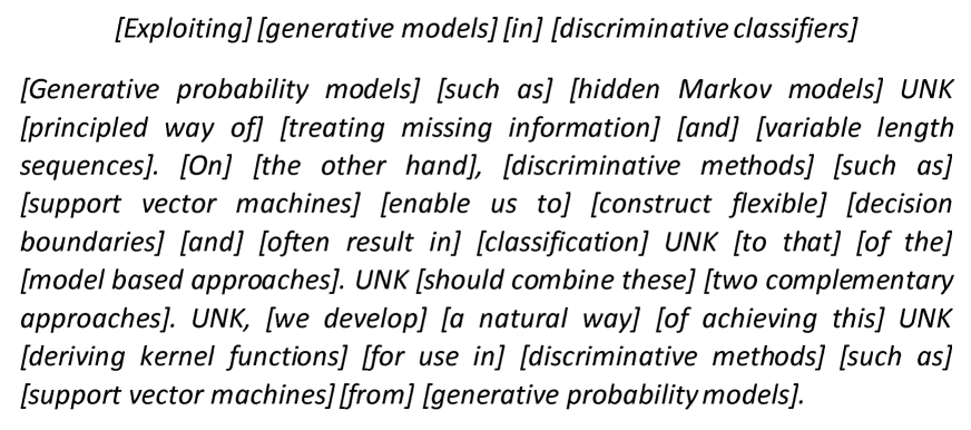
Figure 5: Example text with automatic segmentation, obtained using the path with highest probability. Words in the same brackets “[ ]” belong to the same segment. “UNK” indicates a word not in the vocabulary. The maximum segment length $L=3$.

4.2 Speech recognition

We also apply our model to speech recognition, and present results on both phoneme-level and character-level experiments. This corresponds to an application of SWAN described in Section 2.2.

Dataset.

We evaluate SWAN on the TIMIT corpus following the setup in Deng et al. (2006). The audio data is encoded using a Fourier-transform-based filter-bank with 40 coefficients (plus energy) distributed on a mel-scale, together with their first and second temporal derivatives. Each input vector is therefore size 123. The data is normalized so that every element of the input vectors has zero mean and unit variance over the training set. All 61 phoneme labels are used during training and decoding, then mapped to 39 classes for scoring in the standard way (Lee & Hon, 1989).

Phoneme-level results.

Our SWAN model consists of a $5$-layer bidirectional GRU with 300 hidden units as the encoder and two $2$-layer unidirectional GRU(s) with 600 hidden units, one for the segments and the other for connecting the segments in SWAN. We set the maximum segment length $L=3$. To reduce the temporal input size for SWAN, we add a temporal convolutional layer with stride $2$ and width $2$ at the end of the encoder. For optimization, we largely followed the strategy in Zhang et al. (2017). We use Adam (Kingma & Ba, 2014) with learning rate $4e-4$. We then use stochastic gradient descent with learning rate $3e-5$ for fine-tuning. Batch size $20$ is used during training. We use dropout with probability of $0.3$ across the layers except for the input and output layers. Beam size $40$ is used for decoding. Table 3 shows the results compared with some previous approaches. SWAN achieves competitive results without using a separate alignment tool.

We also examine the properties of SWAN’s outputs. We first estimate the average segment length $\ell$ for the output. We find that $\ell$ is usually smaller than $1.1$ from the settings with good performances. Even when we increase the maximum segment length $L$ to $6$, we still do not see a significantly increase of the average segment length. We suspect that the phoneme labels are relatively independent summarizations of the acoustic features and it is not easy to find good phoneme-level segments. The most common segment patterns we observe are ‘sil ?’, where ‘sil’ is the silence phoneme label and ‘?’ denotes some other phoneme label (Lee & Hon, 1989). On running time, SWAN is about 5 times slower than CTC. (Note that CTC was written in CUDA C, while SWAN is written in torch.)

Table 2: Examples of character-level outputs with their segmentations, where “$\cdot$” represents the segment boundary, “$\square$” represents the space symbol in SWAN’s outputs, the “best path” represents the most probable segmentation given the ground truth, and the “max decoding” represents the beam search decoding result with beam size 1.

ground truth	one thing he thought nobody knows about it yet
best path	o$\cdot$ne$\square$$\cdot$th$\cdot$i$\cdot$ng$\square$$\cdot$he$\square$$\cdot$th$\cdot$ou$\cdot$ght$\cdot$$\square$$\cdot$n$\cdot$o$\cdot$bo$\cdot$d$\cdot$y$\square$$\cdot$kn$\cdot$o$\cdot$w$\cdot$s$\square$$\cdot$a$\cdot$b$\cdot$ou$\cdot$t$\square$$\cdot$i$\cdot$t$\square$$\cdot$y$\cdot$e$\cdot$t
max decoding	o$\cdot$ne$\square$$\cdot$th$\cdot$a$\cdot$n$\cdot$$\square$$\cdot$he$\square$$\cdot$th$\cdot$ou$\cdot$gh$\cdot$o$\cdot$t$\square$$\cdot$n$\cdot$o$\cdot$bo$\cdot$d$\cdot$y$\square$$\cdot$n$\cdot$o$\cdot$se$\square$$\cdot$a$\cdot$b$\cdot$ou$\cdot$t$\square$$\cdot$a$\cdot$t$\square$$\cdot$y$\cdot$e$\cdot$t
ground truth	jeff thought you argued in favor of a centrifuge purchase
best path	j$\cdot$e$\cdot$ff$\cdot$$\square$$\cdot$th$\cdot$ou$\cdot$ght$\square$$\cdot$you$\cdot$$\square$$\cdot$a$\cdot$r$\cdot$g$\cdot$u$\cdot$ed$\square$$\cdot$in$\square$$\cdot$f$\cdot$a$\cdot$vor$\cdot$$\square$$\cdot$of$\square$$\cdot$a$\cdot$$\square$$\cdot$c$\cdot$en$\cdot$tr$\cdot$i$\cdot$f$\cdot$u$\cdot$ge$\square$$\cdot$p$\cdot$ur$\cdot$ch$\cdot$a$\cdot$s$\cdot$e
max decoding	j$\cdot$a$\cdot$ff$\cdot$$\square$$\cdot$th$\cdot$or$\cdot$o$\cdot$d$\cdot$y$\square$$\cdot$a$\cdot$re$\square$$\cdot$g$\cdot$i$\cdot$vi$\cdot$ng$\square$$\cdot$f$\cdot$a$\cdot$ver$\cdot$$\square$$\cdot$of$\square$$\cdot$er$\cdot$s$\cdot$e$\cdot$nt$\cdot$$\square$$\cdot$f$\cdot$u$\cdot$ge$\square$$\cdot$p$\cdot$er$\cdot$ch$\cdot$e$\cdot$s
ground truth	he trembled lest his piece should fail
best path	he$\cdot$$\square$$\cdot$tr$\cdot$e$\cdot$m$\cdot$b$\cdot$le$\cdot$d$\square$$\cdot$l$\cdot$e$\cdot$s$\cdot$t$\cdot$$\square$$\cdot$hi$\cdot$s$\square$$\cdot$p$\cdot$i$\cdot$e$\cdot$ce$\square$$\cdot$sh$\cdot$oul$\cdot$d$\square$$\cdot$f$\cdot$a$\cdot$i$\cdot$l
max decoding	he$\cdot$$\square$$\cdot$tr$\cdot$e$\cdot$m$\cdot$b$\cdot$le$\square$$\cdot$n$\cdot$e$\cdot$s$\cdot$t$\cdot$$\square$$\cdot$hi$\cdot$s$\square$$\cdot$p$\cdot$ea$\cdot$s$\cdot$u$\cdot$de$\square$$\cdot$f$\cdot$a$\cdot$i$\cdot$l

Table 3: TIMIT phoneme recognition results. “PER” is the phoneme error rate on the core test set.

Model	PER (%)
BiLSTM-5L-250H (Graves et al., 2013)	18.4
TRANS-3L-250H (Graves et al., 2013)	18.3
Attention RNN (Chorowski et al., 2015)	17.6
Neural Transducer (Jaitly et al., 2016)	18.2
CNN-10L-maxout (Zhang et al., 2017)	18.2
SWAN (this paper)	18.1

Character-level results.

In additional to phoneme-level recognition experiments, we also evaluate our model on the task to directly output the characters like Amodei et al. (2016). We use the original word level transcription from the TIMIT corpus, convert them into lower cases, and separate them to character level sequences (the vocabulary includes from ‘a’ to ‘z’, apostrophe and the space symbol.) We find that using temporal convolutional layer with stride $7$ and width $7$ at the end of the decoder and setting $L=8$ yields good results. In general, we found that starting with a larger $L$ is useful. We believe that a larger $L$ allows more explorations of different segmentations and thus helps optimization since we consider the marginalization of all possible segmentations. We obtain a character error rate (CER) of ${\bf 30.5\%}$ for SWAN compared to $31.8\%$ for CTC.

We examine the properties of SWAN for this character-level recognition task. Different from the observation from the phoneme-level task, we find the average segment length $\ell$ is around $1.5$ from the settings with good performances, longer than that of the phoneme-level setting. This is expected since the variability of acoustic features for a character is much higher than that for a phone and a longer segment of characters helps reduce that variability. Table 2 shows some example decoding outputs. As we can see, although not perfect, these segments often correspond to important phonotactics rules in the English language and we expect these to get better when we have more labeled speech data. In Figure 6, we show an example of mapping the character-level alignment back to the speech signals, together with the ground truth phonemes. We can observe that the character level sequence roughly corresponds to the phoneme sequence in terms of phonotactics rules.

Finally, from the examples in Table 2, we find that the space symbol is often assigned to a segment together with its preceding character(s) or as an independent segment. We suspect this is because the space symbol itself is more like a separator of segments than a label with actual acoustic meanings. So in future work, we plan to treat the space symbol between words as a known segmentation boundary that all valid segmentations should comply with, which will lead to a smaller set of possible segments. We believe this will not only make it easier to find appropriate segments, but also significantly reduce the computational complexity.

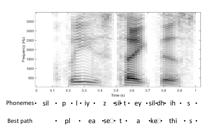
Figure 6: Spectrogram of a test example of the output sequence, “please take this”. Here “$\cdot$” represents the boundary and $\square$ represents the space symbol in SWAN’s result. The “phonemes” sequence is the ground truth phoneme labels. (The full list of phoneme labels and their explanations can be found in Lee & Hon (1989).) The “best path” sequence is from SWAN. Note that the time boundary is not precise due to the convolutional layer.

5 Conclusion and Future work

In this paper, we present a new probability distribution for sequence modeling and demonstrate its usefulness on two different tasks. Due to the generality, it can be used as a loss function in many sequence modeling tasks. We plan to investigate following directions in future work. The first is to validate our approach on large-scale speech datasets. The second is machine translation, where segmentations can be regarded as “phrases.” We believe this approach has the potential to bring together the merits of traditional phrase-based translation (Koehn et al., 2003) and recent neural machine translation (Sutskever et al., 2014; Bahdanau et al., 2014). For example, we can restrict the number of valid segmentations with a known phrase set. Finally, applications in other domains including DNA sequence segmentation (Braun & Muller, 1998) might benefit from our approach as well.

References

- Amodei et al. (2016) Amodei, Dario, Anubhai, Rishita, Battenberg, Eric, Case, Carl, Casper, Jared, Catanzaro, Bryan Diamos, Greg, et al. Deep speech 2: End-to-end speech recognition in English and Mandarin. In Proceedings of the 33rd International Conference on Machine Learning, pp. 173–182, 2016.
- Bahdanau et al. (2014) Bahdanau, Dzmitry, Cho, Kyunghyun, and Bengio, Yoshua. Neural machine translation by jointly learning to align and translate. arXiv preprint arXiv:1409.0473, 2014.
- Blei et al. (2003) Blei, D., Ng, A., and Jordan, M. Latent Dirichlet allocation. Journal of Machine Learning Research, 3:993–1022, January 2003.
- Braun & Muller (1998) Braun, Jerome V and Muller, Hans-Georg. Statistical methods for dna sequence segmentation. Statistical Science, pp. 142–162, 1998.
- Chorowski et al. (2015) Chorowski, Jan K, Bahdanau, Dzmitry, Serdyuk, Dmitriy, Cho, Kyunghyun, and Bengio, Yoshua. Attention-based models for speech recognition. In Advances in Neural Information Processing Systems, pp. 577–585, 2015.
- Chung et al. (2014) Chung, Junyoung, Gulcehre, Caglar, Cho, KyungHyun, and Bengio, Yoshua. Empirical evaluation of gated recurrent neural networks on sequence modeling. arXiv preprint arXiv:1412.3555, 2014.
- Deng & Jaitly (2015) Deng, Li and Jaitly, Navdeep. Deep discriminative and generative models for speech pattern recognition. Chapter 2 in Handbook of Pattern Recognition and Computer Vision (Ed. C.H. Chen), pp. 27–52, 2015.
- Deng et al. (2006) Deng, Li, Yu, Dong, and Acero, Alex. Structured speech modeling. IEEE Trans. Audio, Speech, and Language Processing, pp. 1492–1504, 2006.
- Graves (2012) Graves, Alex. Sequence transduction with recurrent neural networks. arXiv preprint arXiv:1211.3711, 2012.
- Graves (2013) Graves, Alex. Generating sequences with recurrent neural networks. arXiv preprint arXiv:1308.0850, 2013.
- Graves et al. (2006) Graves, Alex, Fernández, Santiago, Gomez, Faustino, and Schmidhuber, Jürgen. Connectionist temporal classification: labelling unsegmented sequence data with recurrent neural networks. In Proceedings of the 23rd international conference on Machine learning, pp. 369–376. ACM, 2006.
- Graves et al. (2013) Graves, Alex, Mohamed, Abdel-rahman, and Hinton, Geoffrey. Speech recognition with deep recurrent neural networks. In IEEE International Conference on Acoustics Speech and Signal Processing (ICASSP),, pp. 6645–6649. IEEE, 2013.
- Hochreiter & Schmidhuber (1997) Hochreiter, Sepp and Schmidhuber, Jürgen. Long short-term memory. Neural Computation, 9(8):1735–1780, 1997.
- Hoffman et al. (2013) Hoffman, M., Blei, D., Wang, C., and Paisley, J. Stochastic variational inference. Journal of Machine Learning Research, 14(1303–1347), 2013.
- Jaitly et al. (2016) Jaitly, Navdeep, Le, Quoc V, Vinyals, Oriol, Sutskever, Ilya, Sussillo, David, and Bengio, Samy. An online sequence-to-sequence model using partial conditioning. In Advances in Neural Information Processing Systems, pp. 5067–5075, 2016.
- Jordan (1999) Jordan, Michael (ed.). Learning in Graphical Models. MIT Press, Cambridge, MA, 1999.
- Kingma & Ba (2014) Kingma, Diederik and Ba, Jimmy. Adam: A method for stochastic optimization. arXiv preprint arXiv:1412.6980, 2014.
- Kingma & Welling (2013) Kingma, Diederik P and Welling, Max. Auto-encoding variational Bayes. arXiv preprint arXiv:1312.6114, 2013.
- Koehn et al. (2003) Koehn, Philipp, Och, Franz Josef, and Marcu, Daniel. Statistical phrase-based translation. In Proceedings of the 2003 Conference of the North American Chapter of the Association for Computational Linguistics on Human Language Technology-Volume 1, pp. 48–54. Association for Computational Linguistics, 2003.
- Kong et al. (2015) Kong, Lingpeng, Dyer, Chris, and Smith, Noah A. Segmental recurrent neural networks. arXiv preprint arXiv:1511.06018, 2015.
- Lee & Hon (1989) Lee, Kai-Fu and Hon, Hsiao-Wuen. Speaker-independent phone recognition using hidden markov models. IEEE Transactions on Acoustics, Speech, and Signal Processing, 37(11):1641–1648, 1989.
- Miao et al. (2016) Miao, Yishu, Yu, Lei, and Blunsom, Phil. Neural variational inference for text processing. In Proceedings of the 33rd International Conference on Machine Learning, pp. 1727–1736, 2016.
- Rezende et al. (2014) Rezende, Danilo Jimenez, Mohamed, Shakir, and Wierstra, Daan. Stochastic backpropagation and approximate inference in deep generative models. In Proceedings of the 31st International Conference on Machine Learning, pp. 1278–1286, 2014.
- Sarawagi & Cohen (2004) Sarawagi, Sunita and Cohen, William W. Semi-markov conditional random fields for information extraction. In In Advances in Neural Information Processing Systems 17, pp. 1185–1192, 2004.
- Sutskever et al. (2014) Sutskever, Ilya, Vinyals, Oriol, and Le, Quoc V. Sequence to sequence learning with neural networks. In Advances in Neural Information Processing Systems, pp. 3104–3112, 2014.
- Wang & Blei (2011) Wang, Chong and Blei, David M. Collaborative topic modeling for recommending scientific articles. In ACM International Conference on Knowledge Discovery and Data Mining, 2011.
- Yu et al. (2016) Yu, Lei, Buys, Jan, and Blunsom, Phil. Online segment to segment neural transduction. arXiv preprint arXiv:1609.08194, 2016.
- Zhang et al. (2017) Zhang, Ying, Pezeshki, Mohammad, Brakel, Philémon, Zhang, Saizheng, Laurent, César, Bengio, Yoshua, and Courville, Aaron. Towards end-to-end speech recognition with deep convolutional neural networks. arXiv preprint arXiv:1701.02720, 2017.