The Glauber model and heavy ion reaction and elastic scattering cross sections

Abstract

We revisit the Glauber model to study the heavy ion reaction cross sections and elastic scattering angular distributions at low and intermediate energies. The Glauber model takes nucleon-nucleon cross sections and nuclear densities as inputs and has no free parameter and thus can predict the cross sections for unknown systems. The Glauber model works at low energies down to Coulomb barrier with very simple modifications. We present new parametrization of measured total cross sections as well as ratio of real to imaginary parts of the scattering amplitudes for pp and np collisions as a function of nucleon kinetic energy. The nuclear (charge) densities obtained by electron scattering form factors measured in large momentum transfer range are used in the calculations. The heavy ion reaction cross sections are calculated for light and heavy systems and are compared with available data measured over large energy range. The model gives excellent description of the data. The elastic scattering angular distributions are calculated for various systems at different energies. The model gives good description of the data at small momentum transfer but the calculations deviate from the data at large momentum transfer.

1 Introduction

The Glauber model [1] is a semi classical model picturing the nuclei moving in a straight line trajectory along the collision direction and describes nucleus-nucleus interaction [2] in terms of nucleon-nucleon (NN) interactions. At high energies it is used to obtain total nucleus-nucleus cross section and geometric properties of the collisions such as the number of participants and binary NN collisions as a function of impact parameter [see e.g. [3, 4, 5]]. At low energies, the straight line trajectory is assumed at the Coulomb distance of closest approach between the two nuclei [6, 7]. The non eikonal nature of the trajectory is taken into account using a simple prescription given in Ref. [8]. This Coulomb Modified Glauber Model (CMGM) has been widely used in the literature [9, 10, 11, 12]. The work in Ref. [13] presents a systematic calculation of reaction cross section using CMGM. The Glauber model has no free parameter and thus has a variety of applications. It is used to extract the radii of unstable nuclei from measured total or reaction cross sections [14, 15, 16]. The Glauber model formalism together with the measured cross section is frequently used as a tool to test various forms of relativistic mean field densities [17, 18, 19]. It is also a useful tool to study the shape deformation of nuclei [20, 21]. The Glauber approach is similar to microscopic optical model approach which is used to study various nuclear reaction mechanisms [22]. The elastic scattering data are mostly interpreted in terms of optical model potential where the real part is commonly taken as double folding potential. Such formalism uses an imaginary potential with three free parameters and reproduces the diffractive patterns up to large angles as shown in the work of Ref. [23] for the elastic scattering of ¹⁶O + ¹⁶O at incident energies ranging from 124 to 1120 MeV. There are numerous attempts to explain the elastic scattering angular distributions of light nuclei using the Glauber model [24]. To have a better agreement with the data, the NN scattering amplitude is modified to include phase variation [25]. The isospin effects in NN scattering process have small impact on the cross sections as shown in the work of Ref. [26] which calculates the reaction cross section at intermediate energy to study the medium effects on NN scattering cross sections. Ref. [27] describes the elastic scattering angular distributions of ¹⁶O + ¹⁶O and ¹²C + ¹²C using an NN phase shift function having three free parameters. A detailed study in the Ref. [28] presents a Monte Carlo Glauber model calculations of angular distributions of elastic scattering of $\alpha$ on light and heavy nuclei. The Monte Carlo approach includes the geometric fluctuations but is expected to give similar results as optical Glauber model at low energies. On comparison with the data this work concludes that the angular distributions can be predicted only up to certain angles. To get a better agreement at higher angles one may require more parameters as in Ref. [27].

In view of the importance and wide applicability of the model, we extend reaction cross section study of work in Ref. [13] for many more systems and collisions energies. We also calculate elastic scattering angular distributions, a study similar to the work of Ref. [28] but for many more systems. The nucleon-nucleon cross sections $\sigma_{nn}$, $\sigma_{pp}$ and $\sigma_{np}$ are the most important inputs in the calculations. We present simple parametrizations for the total cross sections as well for the ratio of real to imaginary parts of the scattering amplitudes for pp and np collisions using a large set of measurements and make a comparison with those available in the literature [7, 29]. The nuclear (charge) densities obtained by electron scattering form factors measured in large momentum transfer range are used in the calculations [30, 31]. For few systems we use three parameter Fermi density (3pF) in contrast to two parameter Fermi (2pF) density and Gaussian densities used in previous studies. The center of mass correction which is important for light systems has also been taken into account [32]. The reaction cross section and the elastic scattering angular distributions are obtained at many energies and are compared with the data to test the reliability of the model and the input parameters for many cases of stable nuclei.

2 The Glauber Model

The Glauber model gives the probability for occurrence of a nucleon-nucleon collision when the nuclei $A$ and $B$ collide at an impact parameter ${\bf b}$ relative to each other which is determined to be [3, 4]

$$T(b)\bar{\sigma}_{NN}=\int\rho_{A}^{z}({\bf b}_{A})d{\bf b}_{A}\,\rho_{B}^{z}({\bf b}_{B})d{\bf b}_{B}\,t({\bf b-b_{A}+b_{B}})\,\,\bar{\sigma}_{NN}.$$ (1)

Here, $\rho_{A}^{z}({\bf b}_{A})$ and $\rho_{B}^{z}({\bf b}_{B})$ are the z-integrated densities of projectile and target nuclei respectively. $t({\bf b})d{\bf b}$ is the probability for having a nucleon-nucleon collision within the transverse area element $d{\bf b}$ when one nucleon approaches at an impact parameter ${\bf b}$ relative to another nucleon. All these distribution functions are normalized to one. Here $\bar{\sigma}_{NN}$ is the average total nucleon nucleon cross section.

The total reaction cross section $\sigma_{R}$ can be written as

$$\sigma_{R} =2\pi\int bdb\left(1-|S(b)|^{2}\right),$$

$$=\frac{\pi}{k^{2}}\,\sum_{l=0}^{\infty}\,(2l+1)(1-|S_{l}|^{2}).$$

The scattering matrix $S_{l}$ or $S(b)$ where $bk=(l+1/2)$ is given by

$$S(b)=\exp\left(i\chi(b)\right).$$ (2)

The Glauber phase shift $\chi(b)$ can be written as

$$\chi(b)={1\over 2}\bar{\sigma}_{NN}(\bar{\alpha}_{NN}+i)\,AB\,\,T(b).$$ (3)

Here, $\bar{\alpha}_{NN}$ is the ratio of real to imaginary part of NN scattering amplitude which does not appear in the calculations of reaction cross section but is important for elastic scattering angular distribution.

In momentum space, $T(b)$ is derived as [13]

$$T(b)={1\over 2\pi}\int J_{0}(qb)S_{A}({\bf q})S_{B}(-{\bf q})f_{NN}(q)qdq.$$ (4)

Here, $S_{A}(q)$ and $S_{B}(-q)$ are the Fourier transforms of the nuclear densities and $J_{0}(qb)=1/2\pi\int\exp(-qb\cos\phi)d\phi$ is the cylindrical Bessel function of zeroth order. The function $f_{NN}(q)$ is the Fourier transform of the profile function $t({\bf b})$ and gives the $q$ dependence of NN scattering amplitude. The profile function $t({\bf b})$ for the NN scattering can be taken as delta function if the nucleons are point particles. In general, it is taken as a Gaussian function of width $r_{0}$ as

$$t({\bf b})={\exp(-b^{2}/2r_{0}^{2})\over(2\pi r_{0}^{2})}.$$ (5)

Thus,

$$f_{NN}(q)=\exp(-r_{0}^{2}q^{2}/2).$$ (6)

Here, $r_{0}$ is the range parameter and has a weak dependence on energy (see for discussions [10]). For the present work, we use $r_{0}=0.6$ fm, which is guided by the previous studies in the same energy region from Refs. [13, 7].

In the presence of Coulomb field, the non eikonal trajectory around the Coulmob distance of closest approach $r_{c}$ is represented by $r^{2}=r_{c}^{2}+(C+1)z^{2}$ [8] where $r_{c}$ and the factor $C$ are given by

$$r_{c}=(\eta+\sqrt{\eta^{2}+b^{2}k^{2}})/k,$$ (7)

$$C=\frac{\eta}{kb^{2}}r_{c}.$$ (8)

Here, $\eta=Z_{P}Z_{T}e^{2}/\hbar v$ is the dimensionless Sommerfield parameter. In the Coulomb Modified Glauber Model (CMGM) the Eq. 3 is modified as

$$\chi(b)={1\over 2}\bar{\sigma}_{NN}(\bar{\alpha}_{NN}+i)\,AB\,\,T(r_{c})/\sqrt{C+1}.$$ (9)

3 Elastic Scattering Cross Section

The nucleus-nucleus differential elastic cross section as a function of center of mass angle $\theta$ is given by

$${\frac{d\sigma_{el}}{d\Omega}}=|f(\theta)|^{2},$$ (10)

where $f(\theta)$ is the sum of Coulomb and nuclear scattering amplitudes.

$$f(\theta)=f_{C}(\theta)+f_{N}(\theta).$$ (11)

For identical systems, the LHS of Eq. 10 is replaced by $|f(\theta)+f(\pi-\theta)|^{2}$. The Coulomb scattering amplitude is given by

$$f_{C}(\theta)=A_{C}\,e^{i\phi_{C}},$$ (12)

where $A_{C}=-{\frac{\eta}{2k}}cosec^{2}{\frac{\theta}{2}}$,   $\phi_{C}=2\sigma_{0}-2\eta\ln\bigg{(}\sin{\frac{\theta}{2}}\bigg{)}$ and the nuclear scattering amplitude is

$$f_{N}(\theta)={\frac{1}{2ik}}\sum_{l=0}^{\infty}(2l+1)(e^{2i\sigma_{l}})(S_{l}-1)P_{l}(\cos\theta).$$ (13)

Here, $\sigma_{l+1}(\eta)=\sigma_{l}(\eta)+tan^{-1}(\frac{\eta}{l+1})$ and $\sigma_{0}$ can be assumed to be 0. The nuclear scattering amplitude can be written as $S_{l}=\exp[i(\chi_{R}+i\chi_{I})]$ and thus $f_{N}(\theta)$ is simplified to

$$f_{N}(\theta)=\frac{1}{2k}\sum_{l=0}^{\infty}\,(2l+1)\,P_{l}(\cos\theta)\,(e^{2i\sigma_{l}})\,[N_{R}+iN_{I}],$$ (14)

where $N_{R}=[e^{-\chi_{I}}\,\sin\chi_{R}]$ and $N_{I}=[1-e^{-\chi_{I}}\,\cos\chi_{R}]$.

4 The Nuclear Densities

Table 1: Density parameters of nuclei used in the present work. The parameters $\alpha$ and $a$ correspond to MHO density, the parameters $d$ and $c$ correspond to 2pF/3pF densities and $\omega$ corresponds to 3pF density. $q$-range is measured momentum transfer range.

Element	Form	$d$/$\alpha$	$R_{rms}$	$c$/$a$	$w$	$q$-range	Ref.
		(fm)	(fm)	(fm)
${}^{12}_{6}$C	MHO	1.247(18)	2.460	1.649(8)		1.05-4.01	[30]
${}^{16}_{8}$O	HO	1.517	2.674	1.805(15)		0.58-0.99	[30]
${}^{28}_{14}$Si	2pF	0.542(16)	3.138	3.106(30)		0.41-2.02	[30]
${}^{40}_{20}$Ca	3pF	0.584	3.486	3.669	-0.102	0.49-3.37	[30]
${}^{90}_{40}$Zr	2pF	0.55	4.274	4.712		-	[13]
${}^{208}_{82}$Pb	2pF	0.549(8)	5.521	6.624(35)		0.22-0.88	[30]

The nuclear densities of the two nuclei are the most important inputs in the model. We can calculate the Fourier transform for any given density form $\rho(r)$ to be used in Eq. (4) as follows

$$S(q)=4\pi\int j_{0}(qr)\,\rho(r)\,r^{2}dr$$ (15)

Here, $j_{0}(qr)$ is the spherical Bessel function of order zero. The nuclear densities are obtained by fitting electron nucleus scattering form factors measured in a momentum transfer range [30, 31]. For light nuclei such as ⁶Li, ¹²C and ¹⁶O, we use the Modified Harmonic Oscillator (MHO) density with correction for center of mass motion [13]. For heavier nuclei such as ²⁸Si, ⁹⁰Zr and ²⁰⁸Pb we use two parameter Fermi (2pF) density. We also use the three parameter Fermi (3pF) density for nuclei such as ⁴⁰Ca for which 2pF density is not given for wide q-range of measured form factor. The mean radius, $c$ for ⁹⁰Zr has been calculated using the formula given in Ref. [13].

The MHO density form is given by

$$\rho(r)=\rho_{0}\bigg{(}1+\alpha\frac{r^{2}}{a^{2}}\bigg{)}\,\exp\bigg{(}-\frac{r^{2}}{a^{2}}\bigg{)}\,,\,\,\,\,\rho_{0}=\frac{1+1.5\alpha}{(\sqrt{\pi}\,a)^{3}}.$$ (16)

The 2pF density is given by

$$\rho(r)=\frac{\rho_{0}}{1+\exp(\frac{r-c}{d})}\,,\,\,\,\,\,\rho_{0}=\frac{3}{4\pi c^{3}[1+\frac{\pi^{2}d^{2}}{c^{2}}]}$$ (17)

and the 3pF density is given by

$$\rho(r)=\frac{\rho_{0}(1+\frac{wr^{2}}{c^{2}})}{1+\exp(\frac{r-c}{d})}.$$ (18)

The parameters for different nuclei used in the present work are given in Table 1.

5 NN scattering parameters

The average NN scattering parameter $\bar{\sigma}_{NN}$ is obtained in terms of pp cross section $\sigma_{pp}$ and np cross section $\sigma_{np}$ averaged over proton numbers ($Z_{P}$, $Z_{T}$) and neutron numbers ($N_{P}$, $N_{T}$) of projectile and target respectively as

$$\bar{\sigma}_{NN}=\frac{N_{P}N_{T}\sigma_{nn}+Z_{P}Z_{T}\sigma_{pp}+(Z_{P}N_{T}+N_{P}Z_{T})\sigma_{np}}{A_{P}A_{T}}.$$ (19)

The parametrized forms of $\sigma_{pp}$ and $\sigma_{np}$ are available in literature [7, 29]. The cross section $\sigma_{pp}$ is assumed to be the same as $\sigma_{pp}$. We obtain new parametrization using the data from Particle Data Group [33] which are given in terms of proton lab kinetic energy $E$ as follows

$$\sigma_{pp}=\left\{\begin{array}[]{ll}-5.32+{3017.0\over E}&:9\leq E({\rm MeV})\leq 90\\ 31.74-0.0628\,E+1.22\times 10^{-4}\,E^{2}&:90\leq E({\rm\,MeV})\leq 700\end{array}\right.,$$ (22)

$$\sigma_{np}=\left\{\begin{array}[]{ll}-1128.0-{863.0\over E}+61.5\sqrt{E}+{6170.0\over\sqrt{E}}&:0.45\leq E({\rm MeV})\leq 70\\ -8.54+{9956.0\over E}+1.64\sqrt{E}-{321.0\over\sqrt{E}}&:70\leq E({\rm MeV})\leq 700\end{array}\right.$$ (25)

The errors on the parameters in Eqs. (22) and (25) are 1-3 %. Figure 1 shows the NN cross section data [33] as a function of lab kinetic energy fitted with the functions given by Eqs. (22) and (25) along with the fits given in references [7, 29]. The data/fit graphs are shown for the present parametrizations. The Charagi-Gupta parametrization for $\sigma_{pp}$ is good upto 50 MeV and that for $\sigma_{np}$ is good above 10 MeV. The Bertulani-Conti parametrization of $\sigma_{pp}$ differs with our parametrizations in the proton energy range 120-300 MeV and their parametrization of $\sigma_{np}$ cannot be extrapolated below 8 MeV.

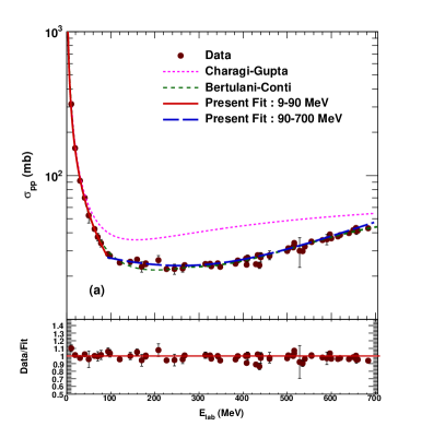
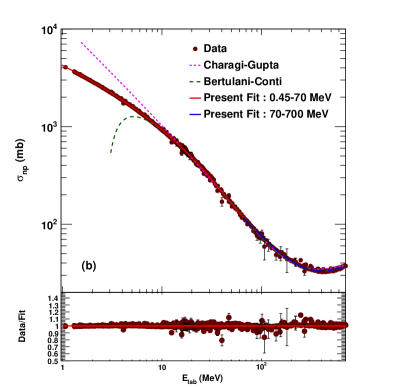
Figure 1: (a) proton-proton cross section and (b) neutron-proton cross section data as a function of lab kinetic energy [33] fitted with the functions given by Eqs. (22) and (25) along with the fits which are given in references [7, 29].

The average $\bar{\alpha}_{NN}$ is also calculated using $\alpha_{pp}$, $\alpha_{nn}$ and $\alpha_{np}$ as follows

$$\bar{\alpha}_{NN}=\frac{N_{P}N_{T}\alpha_{nn}\sigma_{nn}+Z_{P}Z_{T}\alpha_{pp}\sigma_{pp}+(Z_{P}N_{T}+N_{P}Z_{T})\alpha_{np}\sigma_{np}}{\sigma_{NN}A_{P}A_{T}}.$$ (26)

The parametrizations for quantities $\alpha_{pp}$ and $\alpha_{np}$ as a function of lab kinetic energy are obtained using the data of phase shift analysis given in Ref. [34] which is in accordance with the experimental data. It is assumed that $\alpha_{nn}$ = $\alpha_{pp}$. The present parametrizations are obtained for proton lab energy $E$ between 7 to 260 MeV given as

$$\alpha_{pp}=a_{p}+b_{p}E+c_{p}E^{2}+d_{p}E^{3}\,\,\,\,E\,\,({\rm in\,MeV}),$$ (27)

where $a_{p}=0.435$, $b_{p}=3.202\times 10^{-2}$, $c_{p}=-2.287\times 10^{-4}$ and $d_{p}=4.134\times 10^{-7}$ and

$$\alpha_{np}=a_{n}+b_{n}E+c_{n}E^{2}+d_{n}E^{3}\,\,\,\,E\,({\rm in\,MeV}),$$ (28)

where $a_{n}=-0.3695$, $b_{n}=3.211\times 10^{-2}$, $c_{n}=-2.117\times 10^{-4}$ and $d_{n}=3.672\times 10^{-7}$. The errors on these parameters are 7-10 %.

Figure 2 shows the ratio of real to imaginary part of NN scattering amplitude as a function of lab kinetic energy from phase shift analysis of Ref. [34] fitted with the functions given by Eqs. (27) and (28) along with the fit which was given in Ref. [7]. The earlier parametrization [7] for $\alpha_{pp}$ and $\alpha_{np}$ were good below 60 MeV.

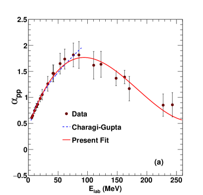
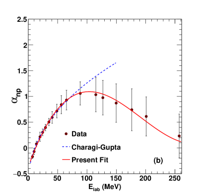
Figure 2: The ratio of real to imaginary part of NN scattering amplitude (a) $\alpha_{pp}$ and (b) $\alpha_{np}$ as a function of lab kinetic energy obtained from phase shift analysis of Ref. [34] fitted with the functions given by Eqs. (27) and (28) along with the fit which was given in Ref. [7].

6 Results and discussions

We calculate $\sigma_{R}$ as a function of lab kinetic energy per nucleon $E/A$ and $\frac{d\sigma_{el}}{d\sigma_{Ruth}}$ as a function of $\theta_{\rm cm}$ for various reaction combinations of light, medium and heavy nuclei and compare with the data. The reaction cross section data are obtained by optical model analysis of measured elastic scattering angular distributions. Such analysis is mostly provided by the experimental group. In case the error on the cross section is not given a 5 % error is assumed which is typically the error obtained in such analysis. The errors on the input parameters, NN cross sections and density parameters are propagated in the final calculations. The uncertainty bands also include an 8 % variation in the nuclear range parameter $r_{0}$ arround 0.6 fm.

Figure 3 shows the total reaction cross section as a function of lab kinetic energy per nucleon for ¹²C + ¹²C system [35, 36, 37]. For this system we have put 5 % error on the cross section data at $E/A$ = 8.567, 30 and 120.75 MeV. Figure 4 (a) shows the total reaction cross section as a function of lab kinetic energy per nucleon for ¹⁶O + ¹⁶O system [38, 39, 40] and the Fig. 4 (b) shows the same for ¹⁶O + ¹²C system [41, 42, 43, 44, 45, 46]. The band is CMGM which includes the uncertainties on the input parameters. The model gives very good description of the data for all the light systems except at very low energies far below Coulomb barrier for ¹⁶O + ¹⁶O system.

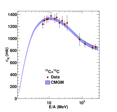
Figure 3: The total reaction cross section as a function of lab kinetic energy per nucleon for ¹²C + ¹²C system [35, 36, 37].

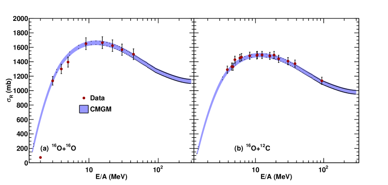
Figure 4: The total reaction cross section as a function of lab kinetic energy per nucleon for (a) ¹⁶O + ¹⁶O system [38, 39, 40] and (b) ¹⁶O + ¹²C system [41, 42, 43, 44, 45, 46].

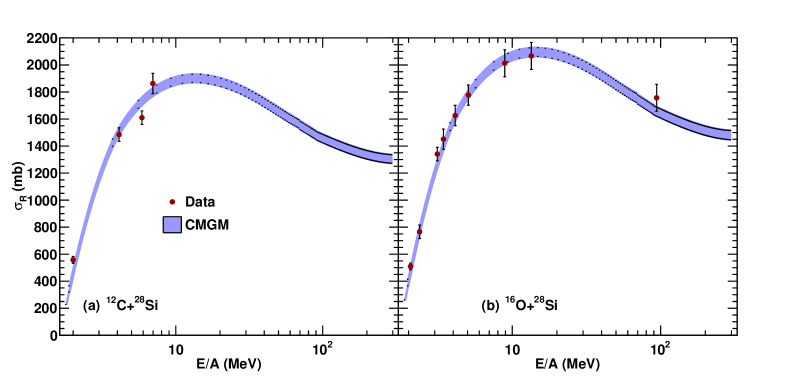
Figure 5: The total reaction cross section as a function of lab kinetic energy per nucleon for (a) ¹²C + ²⁸Si system [42] and (b) ¹⁶O + ²⁸Si system [47].

Figure 5 (a) shows the total reaction cross section as a function of lab kinetic energy per nucleon for ¹²C + ²⁸Si system [42] and the Fig. 5 (b) shows the same for ¹⁶O + ²⁸Si system [47]. For all the data shown in figures 4 and 5 we have put 5 % error on the reaction cross section. Figure 6 (a) shows the total reaction cross section as a function of lab kinetic energy per nucleon for ¹²C + ⁴⁰Ca system [35, 44] and the Fig. 6 (b) shows the same for ¹²C + ⁹⁰Zr system [35, 44, 48]. The band is CMGM which includes the uncertainties on the input parameters. The model gives good description of the data for medium mass systems except for the ¹²C + ⁹⁰Zr system. For ¹²C + ⁴⁰Ca system at energy $E/A$ = 3.75 MeV we have put a 5 % error on the reaction cross section. Similar error was put in the cross section for the system ¹²C + ⁹⁰Zr at energies $E/A$ = 8.166 and 35 MeV.

Figure 7 (a) shows the total reaction cross section as a function of lab kinetic energy per nucleon for ¹²C + ²⁰⁸Pb system [35, 48, 49]. Figure 7 (b) shows the same for ¹⁶O + ²⁰⁸Pb system [50, 51, 52, 53, 54, 55]. The band is CMGM which includes the uncertainties on the input parameters. For ¹²C + ²⁰⁸Pb system at energies $E/A$ = 8 and 9.66 MeV we have put a 5 % error on the reaction cross section. Similar error was put in the cross section for the system ¹⁶O + ²⁰⁸Pb at energies $E/A$ = 6.0, 8.093, 12.0 and 19.54 MeV.

The model gives very good description of the data for both the heavy systems considered here. We can conclude that the reaction cross section calculations from the model are very reliable and and thus the model can be used to predict the reaction cross section for unknown systems. It can also be used to obtain radii of nuclei from measured reaction cross section.

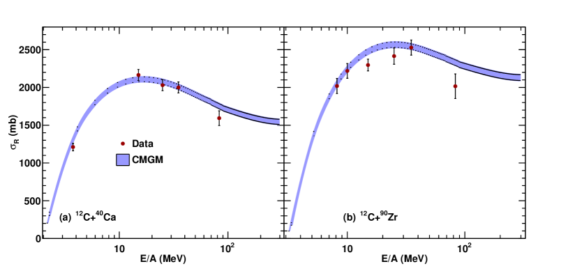
Figure 6: The total reaction cross section as a function of lab kinetic energy per nucleon for (a) ¹²C + ⁴⁰Ca system [35, 44] and (b) ¹²C + ⁹⁰Zr system [35, 44, 48].

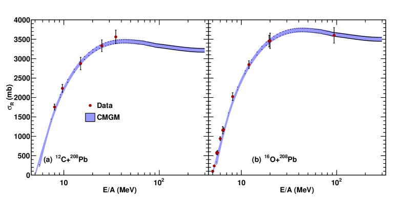
Figure 7: The total reaction cross section as a function of lab kinetic energy per nucleon for (a) ¹²C + ²⁰⁸Pb system [35, 48, 49] and (b) ¹⁶O + ²⁰⁸Pb system [50, 51, 52, 53, 54, 55, 46].

Figures 8 shows the measured ratio of elastic scattering cross section to the Rutherford cross section as a function of scattering angle for ¹²C + ¹²C system at three energies given in (a) $E/A$ = 15 MeV [56], (b) $E/A$ = 30 MeV [49, 57, 58] and (c) $E/A$ = 84.66 MeV [49, 57] along with the CMGM calculations shown by bands. Figure 9 shows the measured ratio of elastic scattering cross section to the Rutherford cross section as a function of scattering angle for ¹⁶O + ¹⁶O system for three energies given in (a) $E/A$ = 8.12 MeV [59] (b) $E/A$ = 44 MeV [60, 61] and (c) $E/A$ = 70 MeV [60] along with the CMGM calculations shown by bands.

The parameter $\bar{\alpha}_{NN}$ is obtained by fitting the experimental data on angular distribution which is given in the Table 2 along with the values obtained using parametrizations given by Eqs. (27) and (28). The model produces the measured diffractive oscillations but the oscillation magnitudes in the data in the light systems are more pronounced as compared to the oscillations observed in the data specially at higher energies and higher angles i.e. at the higher momentum transfer. The parameter $\bar{\alpha}_{NN}$ does not control oscillation magnitude, but affects the slope (inclination) of $d\sigma/d\sigma_{Ruth}$ as a function of $\theta_{cm}$.

Figure 10 shows the measured ratio of elastic scattering cross section to the Rutherford cross section as a function of scattering angle for ¹²C + ⁴⁰Ca system [35] for two energies given in (a) $E/A$ = 25 MeV and (b) $E/A$ = 35 MeV along with the CMGM calculations shown by bands.

Figure 11 shows the measured ratio of elastic scattering cross section to the Rutherford cross section as a function of scattering angle for ¹²C + ⁹⁰Zr system [35] for two energies given in (a) $E/A$ = 15 MeV and (b) $E/A$ = 35 MeV along with the CMGM calculations shown by bands.

Figure 12 shows the measured ratio of elastic scattering cross section to the Rutherford cross section as a function of scattering angle for ¹²C + ²⁰⁸Pb system [35, 62] for two energies given in (a) $E/A$ = 25 MeV and (b) $E/A$ = 85.83 MeV along with the CMGM calculations shown by bands.

Figure 13 shows the measured ratio of elastic scattering cross section to the Rutherford cross section as a function of scattering angle for ¹⁶O + ²⁰⁸Pb system [53, 46] for two energies given in (a) $E/A$ = 12 MeV and (b) $E/A$ = 93.75 MeV along with the CMGM calculations shown by bands.

The fitted values of the parameter $\bar{\alpha}_{NN}$ for all the systems are given in the Table 2. For heavy ion systems this parameter does not follow the same energy dependence shown by NN scattering and approaches towards one for all the systems. The model produces the measured elastic scattering angular distributions for medium and heavy systems at low energies but, at higher energies the model produces diffractive oscillations of larger magnitude as compared to the data.

The large oscillations in the model at high momentum transfer may be the consequence of assuming a semiclassical picture of scattering in terms of impact parameter and distance of closest approach. The Glauber optical potential in terms of densities of the two nuclei and NN amplitude does not always reproduce the features of data at large scattering angles. An improved fitting should be obtained by having more free parameters in the nuclear potential/interactions shown in the studies in Ref. [23] or in Ref. [27].

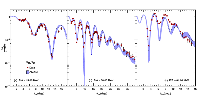
Figure 8: The measured ratio of elastic scattering cross section to the Rutherford cross section as a function of scattering angle for ¹²C + ¹²C system at (a) $E/A$ = 15 MeV [56], (b) $E/A$ = 30 MeV [49, 57, 58] and (c) $E/A$ = 84.66 MeV [49, 57] along with the CMGM calculations.

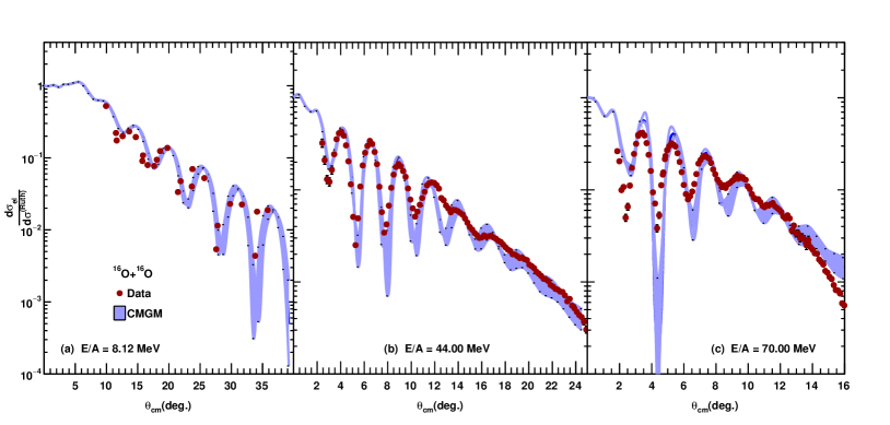
Figure 9: The measured ratio of elastic scattering cross section to the Rutherford cross section as a function of scattering angle for ¹⁶O + ¹⁶O system at (a) $E/A$ = 8.12 MeV [59] (b) $E/A$ = 44 MeV [60, 61] and (c) $E/A$ = 70 MeV [60] along with the CMGM calculations.

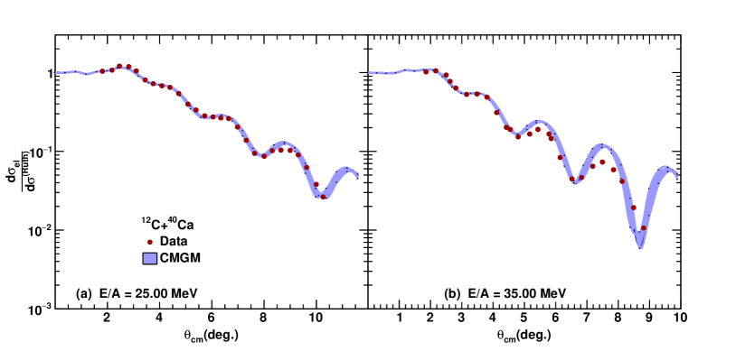
Figure 10: The measured ratio of elastic scattering cross section to the Rutherford cross section as a function of scattering angle for ¹²C + ⁴⁰Ca system [35] at (a) $E/A$ = 25 MeV and (b) $E/A$ = 35 MeV along with the CMGM calculations shown by bands.

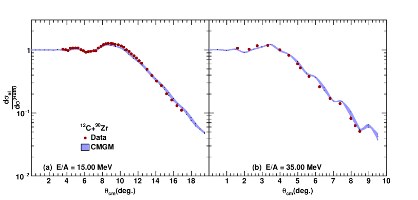
Figure 11: The measured ratio of elastic scattering cross section to the Rutherford cross section as a function of scattering angle for ¹²C + ⁹⁰Zr system [35] at (a) $E/A$ = 15 MeV and (b) $E/A$ = 35 MeV along with the CMGM calculations shown by bands.

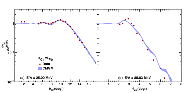
Figure 12: The measured ratio of elastic scattering cross section to the Rutherford cross section as a function of scattering angle for ¹²C + ²⁰⁸Pb system [35, 62] at (a) $E/A$ = 25 MeV and (b) $E/A$ = 85.83 MeV along with the CMGM calculations shown by bands.

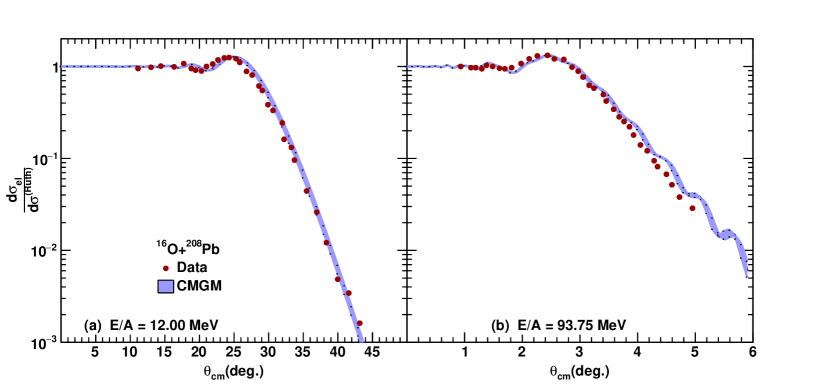
Figure 13: The measured ratio of elastic scattering cross section to the Rutherford cross section as a function of scattering angle for ¹⁶O + ²⁰⁸Pb system [53, 46] at (a) $E/A$ = 12 MeV and (b) $E/A$ = 93.75 MeV along with the CMGM calculations shown by bands.

Table 2: Calculated (from parametrization) and fitted values of $\bar{\alpha}_{NN}$.

System	$E/A$ (MeV)	$\bar{\alpha}_{\rm NN(calc)}$	$\bar{\alpha}_{\rm NN(fitted)}$
12C + 12C	15.00	0.255	0.9
	30.00	0.595	0.78
	84.66	1.25	0.9
16O + 16O	8.12	0.1	0.80
	44.00	0.85	0.94
	70.00	1.165	1.02
12C + 40Ca	25.00	0.488	0.8
	35.00	0.694	1.0
12C + 90Zr	15.00	0.255	0.7
	35.00	0.694	1.0
12C + 208Pb	25.00	0.48	1.0
	85.83	1.25	1.254
16O + 208Pb	12.00	0.181	1.0
	93.75	1.272	1.5

7 Conclusions

We calculate the heavy ion reaction cross sections and elastic scattering angular distributions at low and intermediate energies using Glauber model and test the calculations with the available measured data. We present new parametrization for the data of total cross sections as well as for the ratio of real to imaginary parts of the scattering amplitudes in case of pp and np collisions. The model works at low energies down to Coulomb barrier with very simple modifications. The reaction cross section calculations from the model are very reliable and thus the model can be used to predict the reaction cross section for unknown systems. It can also be used to obtain radii of nuclei from measured reaction cross sections in low and intermediate energy range.

The model describes the measured elastic scattering angular distributions having diffractive oscillations but the oscillation magnitude in the data is more pronounced as compared to the oscillations observed in the data specially at higher energies and higher angles i.e. at the higher momentum transfer. For heavy ion systems, the parameter $\bar{\alpha}_{NN}$ does not follow the same energy dependence shown by NN scattering and approaches towards one for all the systems.

References

References

- [1] R. J. Glauber, Lectures on theoretical Physics, Vol. I, Inter-Science, New York (1959).
- [2] P. J. Karol, Phys. Rev. C11 (1975) 1203.
- [3] C.Y. Wong, Introduction to High Energy Heavy Ion Collisions, World Scientific, Singapore (1994).
- [4] P. Shukla, Preprint: nucl-th/0112039 (2001).
- [5] D. G. d’Enterria, nucl-ex/0302016.
- [6] A. Vitturi and F. Zardi, Phys. Rev. C36 (1987) 1404; S.M. Lenzi, A. Vitturi, F. Zardi, Phys. Rev. C40 (1989) 2114.
- [7] S. K. Charagi and S. K. Gupta, Phys. Rev. C41 (1990) 1610; Phys. Rev. C46 (1992) 1982.
- [8] S. K. Gupta and P. Shukla, Phys. Rev. C52 (1995) 3212.
- [9] R. E. Warner, M. H. McKinnon, and H. Thirumurthy and A. Nadasen, Phys. Rev. C59 (1999) 1215.
- [10] I. Ahmad, M. A. Abdulmomen, and M. S. Al-Enazi, Phys. Rev. C65 (2002) 054607.
- [11] X. Z. Cai, J. Feng, W. Q. Shen, Y. G. Ma, J. S. Wang and W. Ye, Phys. Rev. C 58 (1998) 572.
- [12] A. de Vismes, P. Roussel-Chomaz, and F. Carstoiu, Phys. Rev. C62 (2000) 064612.
- [13] P. Shukla, Phy. Rev. C67 (2003) 054607.
- [14] G. D. Alkhazovi, Y. Shabelski and I. S. Novikov, Int. J. Mod. Phys. E 20 (2011) 583 [arXiv:1101.4717 [nucl-th]].
- [15] I. Tanihata et al., Phys. Rev. Lett. 55 (1985) 2676; I. Tanihata, Nucl. Phys. A488 (1988) 113c; I. Tanihata et. al, Phys. Lett. B289 (1992) 261.
- [16] W. Horiuchi, Y. Suzuki, B. Abu-Ibrahim and A. Kohama, Phys. Rev. C 75 (2007) 044607. Erratum: [Phys. Rev. C 76 (2007) 039903]. [nucl-th/0612029].
- [17] S. K. Patra, R. N. Panda, P. Arumugam and R. K. Gupta, Phys. Rev. C80 (2009) 064602.
- [18] M. K. Sharma and S. K. Patra, Phys. Rev. C87 (2013) 044606.
- [19] D. Chauhan, Z. A. Khan and A. A. Usmani, Phys. Rev. C 90 (2014) 024603.
- [20] M. Y. M. Hassan, M. Y. H. Farag, A. Y. Abul-Magd and T. E. I. Nassar, Phys. Scripta 78 (2008) 045202 [arXiv:0902.0453 [nucl-th]].
- [21] J. A. Christley and J. A. Tostevin, Phys. Rev. C 59 (1999) 2309.
- [22] V. K. Lukyanov, D. N. Kadrev, E. V. Zemlyanaya, K. Spasova, K. V. Lukyanov, A. N. Antonov and M. K. Gaidarov, Phys. Rev. C 91 (2015) 034606. [arXiv: 1502.06425 [nucl-th]].
- [23] Dao T. Khoa, W. von Oertzen, H. G. Bohlena and F. Nuofferc, Nucl. Phys. A 672 (2000) 387.
- [24] M. M. H. El-Gogary, A. S. Shalaby, M. Y. M. Hassan and A. M. Hegazy, Phys. Rev. C 61 (2000) 044604.
- [25] M. M. H. El-Gogary, A. S. Shalaby and M. Y. M. Hassan, Phys. Rev. C 58 (1998) 3513.
- [26] F. Sammarruca and L. White, Phys. Rev. C 83 (2011) 064602. [arXiv: 1105.5666 [nucl-th]].
- [27] I. AHMAD and M. A. ALVI, Int. J. Mod. Phys. E 13 (2000) 1225.
- [28] W. R. Gibbs and J. P. Dedonder, Phys. Rev. C 86 (2012) 024604. [arXiv: 1203.0019 [nucl-th]].
- [29] C. A. Bertulani and C. De Conti, Phys. Rev. C 81 (2010) 064603. [arXiv:1004.2096 [nucl-th]].
- [30] C. W. de Jager, H. de Vries and C. de Vries, Atom. Nucl. Data Tables 14 (1974) 479.
- [31] H. De Vries, C. W. de Jager, and C. de Vries, Atom. Nucl. Data Tables 36 (1987) 495.
- [32] V. Franco and A. Tekou, Phys. Rev. C16 (1987) 658.
- [33] Particle Data Group, (http://pdg.lbl.gov/2014/hadronic-xsections/).
- [34] W. Grein, Nucl. Phys. B131 (1977) 255.
- [35] C. C. Sahm et. al, Phys. Rev. C34 (1986) 2165.
- [36] M. A. Hassanain, A. A. Ibraheem and M. E. Farid, Phys. Rev. C 77 (2008) 034601.
- [37] J. Y. Histachy et. al, Nucl. Phys. A490 (1998) 441.
- [38] R. Bass, Nuclear reactions with heavy ions, (Springer-Verlag, NY), 1980.
- [39] Dao T. Khoa, W. von Oertzen, H. G. Bohlen, G. Bartnitzky, H. Clement, Y. Sugiyama, B. Gebauer, A. N. Ostrowski, Th. Wilpert, M. Wilpert, and C. Langner, Phys. Rev. Lett. 74 (1995) 34.
- [40] M. A. Hassanain, A. A. Ibraheem, S. M. M. Al Sebiey, S. R. Mokhtar, M. A. Zaki, Z. M. M. Mahmoud, K. O. Behairy and M. E. Farid, Phys. Rev. C87 (2013) 064606.
- [41] M. P. Nicoli, F. Haas, R. M. Freeman, S. Szilner, Z. Basrak, A. Morsad, G. R. Satchler and M. E. Brandan, Phys. Rev. C61 (2000) 034609.
- [42] M. El-Azab Farid, Z. M. M. Mahmoud and G.S. Hassan, Nucl. Phys. A691 (2001) 671.
- [43] A. A. Ogloblin et. al, Phys. Rev. C62 (2000) 044601.
- [44] G. R. Satchler and W.G. Love, Phys. Rep. 55 (1979) 183.
- [45] M. E. Brandan et. al, Nucl. Phys. A688 (2001) 659.
- [46] P. Roussel-Chomaz et. al, Nucl. Phys. A477 (1988) 345.
- [47] J.G. Cramer, R.M. Devries, D.A. Goldberg, M.A. Zisman and C.F. Maguire, Phys. Rev. C14 (1976) 2158.
- [48] M. E. Brandan, H. Chehime and K. W. McVoy, Phys. Rev. C55 (1997) 1353.
- [49] M. Buenerd et. al, Phys. Lett. B102 (1981) 242.
- [50] Louis C. Vaz, John M. Alexander, E. H. Auerbach, Phys. Rev. C18 (1978) 820.
- [51] F. D. Becheti, Phys. Rev. C6 (1972) 2215.
- [52] J. B. Ball, C. B. Fulmer, E. E. Gross, M. L. Halbert, D. C. Hensley, C. A. Ludemann, M. J. Saltmarsh and G. R. Satchler, Nucl. Phys. A252 (1975) 208.
- [53] S. K. Charagi, Phys. Rev. C51 (1995) 3521.
- [54] C. Olmer et.al, Phys. Rev.18 (1978) 205.
- [55] K. W. McVoy and W. A. Friedman, Theoretical Methods in Medium-Energy and Heavy-Ion Physics, Springer US (1978).
- [56] Dao T. Khoa, W. von Oertzen, and H. G. Bohlen, Phys. Rev. C 49 (1994) 1652.
- [57] M. Buenerd et. al, Phys. Rev. C26 (1982) 1299.
- [58] M. C. Mermaz, Nucl. Phys. A424 (1984) 313.
- [59] H. Ikezoe et. al, Nucl. Phys. A456 (1986) 298.
- [60] F. Nuoffer et. al, Nuovo Cimento A111 (1998) 971.
- [61] G. Bartnitzky et. al, Phys. Lett. B365 (1996) 23.
- [62] M. A. G. Alvarez, L. C. Chamon, M. S. Hussein, D. Pereira, L. R. Gasques, E. S. Rossi, Jr. and C. P. Silva, Nucl. Phys. A 723 (2003) 93. [nucl-th/0210062].