Optimal Bayesian Minimax Rates for Unconstrained Large Covariance Matrices

Abstract

We obtain the optimal Bayesian minimax rate for the unconstrained large covariance matrix of multivariate normal sample with mean zero, when both the sample size, $n$, and the dimension, $p$, of the covariance matrix tend to infinity. Traditionally the posterior convergence rate is used to compare the frequentist asymptotic performance of priors, but defining the optimality with it is elusive. We propose a new decision theoretic framework for prior selection and define Bayesian minimax rate. Under the proposed framework, we obtain the optimal Bayesian minimax rate for the spectral norm for all rates of $p$. We also considered Frobenius norm, Bregman divergence and squared log-determinant loss and obtain the optimal Bayesian minimax rate under certain rate conditions on $p$. A simulation study is conducted to support the theoretical results.

Key words: Bayesian minimax rate; Convergence rate; Decision theoretic prior selection; Unconstrained covariance.

1 Introduction

Estimating covariance matrix plays a fundamental role in multivariate data analysis. Many statistical methods in multivariate data analysis such as the principle component analysis, canonical correlation analysis, linear and quadratic discriminant analysis require the estimated covariance matrix as the starting point of the analysis. In the risk management and the longitudinal data analysis, the covariance matrix estimation is a crucial part of the analysis. The log-determinant of covariance matrix is used for constructing hypothesis test or quadratic discriminant analysis [2].

Suppose we observe a random sample ${\bf X}_{n}=(X_{1},\ldots,X_{n}),~{}X_{i}\in\mathbb{R}^{p},~{}i=1,\ldots,n,$ from the $p$-dimensional normal distribution with mean zero and covariance matrix $\Sigma$, i.e.

$$X_{1},\ldots,X_{n}\mid\Sigma \overset{iid}{\sim} N_{p}(0,\Sigma).$$

We assume the zero mean and focus on the covariance matrix.

With advance of technology, data arising from various areas such as climate prediction, image processing, gene association study, and proteomics, are often high dimensional. In such high dimensional settings, it is often natural to assume that the dimension of the variable $p$ tends to infinity as the sample size $n$ gets larger, i.e. $p=p_{n}\longrightarrow\infty$ as $n\longrightarrow\infty$. This assumption can be justified as follows. First, when $p$ is large in comparison with $n$, often the limiting scenario with $p$ tending to infinity approximates closer to the reality than that with $p$ fixed. Second, in many cases we can postulate the reality is infinitely complex and involves infinitely many variables, and with limited resources and time, we can collect only a portion of variables and observations. If we have more resources to collect more data, it is natural to collect more observations as well as more variables, i.e. to increase both $n$ and $p$.

When $p$ tends to infinity as $n\longrightarrow\infty$, the traditional covariance estimator is not optimal [32]. The sparsity or bandable assumptions on large matrices have been used frequently in the literature. Many researchers have studied the large sample properties under the restrictive matrix classes. [6] considered the bandable covariance/precision classes and studied the convergence rate of banding estimator on those classes. [44] derived the convergence rate for precision matrices via sparse Cholesky factors and showed that it is the minimax rate under the Frobenius norm. In addition, the minimax convergence rates for the sparse or bandable covariance matrices were established by [11], [12, 13] and [45]. For a comprehensive review on the convergence rate for the covariance and precision matrices, see [10].

The posterior convergence rate has been investigated by [36], [4], and [21]. [36] showed that their continuous shrinkage priors are optimal for the sparse covariance estimation under the spectral norm in the sense that the posterior convergence rate is quite close to the frequentist minimax rate. They achieved a nearly minimax rate upto a $\sqrt{\log n}$ term under the spectral norm and sparse assumption even when $n=o(p)$. [4] considered Bayesian banded precision matrix estimation using graphical models. They obtained the posterior convergence rate of the precision matrix under matrix $\ell_{\infty}$ norm when $\log p=o(n)$. [21] developed a prior distribution for the sparse PCA and showed that it achieves the minimax rate under the Frobenius norm. They also derived the posterior convergence rate under the spectral norm.

Most of the previous works on the Bayesian estimation of large covariance matrix concentrate on the constrained covariance or precision matrix. To the best of our knowledge, only [22] considered asymptotic results for large unconstrained covariance matrix under the “large p and large n” setting. However, they attained the Bernstein-von Mises theorems under somewhat restrictive assumptions on the dimension $p$.

In this paper, we fill the gap in the literature. At first, we propose a new decision theoretic framework to define Bayesian minimax rate. The posterior convergence rate is the primary concept when the asymptotic optimality is studied in the Bayesian sense. But it is not completely satisfactory. The following is a quote from [24] which they write just after defining the posterior convergence rate.

‘We defined “a” rather than the rate of contraction, and hence logically any rate slower than a contraction rate is also a contraction rate. Naturally we are interested in a fastest decreasing sequence $\epsilon_{n}$, but in general this may not exist or may be hard to establish. Thus our rate is an upper bound for a targeted rate, and generally we are happy if our rate is equal to or close to an “optimal” rate. With an abuse of terminology we often make statements like “$\epsilon_{n}$ is the rate of contraction.” ’

In the proposed new decision theoretic framework, a probability measure on the parameter space is an action and a prior is a decision rule for it gives a probability measure (the posterior) for a given data set. In this setup, we define the convergence rate and the Bayesian minimax rate.

We investigate the Bayesian minimax rates for unconstrained large covariance matrix. We consider four losses for the covariance inference: spectral norm, Frobenius norm, Bregman divergence and squared log-determinant loss. For the spectral norm, we have the complete result of the Bayesian minimax rate. We show that the Bayesian minimax rate is $\min(p/n,1)$ for all rates of $p$. For the Frobenius norm and Bregman divergence, we show the Bayesian minimax lower bound is $p\cdot\min(p,\sqrt{n})/n$ for all rates of $p$, but obtained the upper bound under the constraint $p\leq\sqrt{n}$. Thus, under the condition $p\leq\sqrt{n}$, the Bayesian minimax rate is $p^{2}/n.$ We also show that the Bayesian minimax rate under the squared log-determinant loss is $p/n$ when $p=o(n)$.

The rest of the paper is organized as follows. In section 2, we define the model, the covariance classes we consider, and introduce some notations. We propose the new decision theoretical framework and define the Bayesian minimax rate. The Bayesian minimax rates under the spectral norm, the Frobenious norm, the Bregman matrix divergence, and the squared log-determinant loss are presented in section 3. A simulation study is given in section 4. The discussion is given in section 5, and the proofs are given in Supplementary Material ([35]).

2 Preliminaries

2.1 The Model and the Inverse-Wishart Prior

Suppose we observe a random sample from the $p$-dimensional normal distribution

$$X_{1},\cdots,X_{n}\mid\Sigma_{n} \overset{iid}{\sim} N_{p}(0,\Sigma_{n}),$$ (1)

where $\Sigma_{n}$ is a $p\times p$ positive definite matrix, and $p$ is a function of $n$ such that $p=p_{n}\longrightarrow\infty$ as $n\longrightarrow\infty$. The true value of the covariance matrix is denoted by $\Sigma_{0}$ or $\Sigma_{0n}$, which is dependent on $n$.

For the prior of the covariance matrix $\Sigma_{n}$ in model (1), we consider the inverse-Wishart prior

$$\Sigma_{n} \sim IW_{p}(\nu_{n},A_{n}),$$ (2)

where $\nu_{n}>p-1$, $A_{n}$ is a $p\times p$ positive definite matrix for a proper prior. The mean of $\Sigma_{n}$ is $A_{n}/(\nu_{n}-p-1)$. The condition $\nu_{n}>p-1$ is needed for the distribution to have a density in the space of $p\times p$ positive definite matrices. If $\nu_{n}$ is an integer with $\nu_{n}\leq p-1$, (2) defines a singular distribution on the space of $p\times p$ positive semidefinite matrices [43].

We also consider the truncated inverse-Wishart prior. The inverse-Wishart prior with parameter $\nu$ and $A$ whose eigenvalues are restricted in $[K_{1},K_{2}]$ with $0<K_{1}<K_{2}$ is denoted by $IW_{p}(\nu,A,K_{1},K_{2})$. The truncated inverse-Wishart prior was adopted for technical reason. By Lemma E.1, to connect the Frobenius norm with Bregman matrix divergence, the eigenvalues of argument matrices have to be bounded. The truncated inverse-Wishart prior guarantees that the posterior covariance matrix has bounded eigenvalues.

2.2 Matrix Norms and Notations

We define the spectral norm (or matrix $\ell_{2}$ norm) for matrices by

$$\|A\|:=\sup_{\|x\|_{2}=1}\|Ax\|_{2},$$

where $\|\cdot\|_{2}$ denotes the vector $\ell_{2}$ norm defined by $\|x\|_{2}:=(\sum_{i=1}^{p}x_{i}^{2})^{1/2}$, $x=(x_{1},\ldots,x_{p})^{T}\in\mathbb{R}^{p}$ and $A$ is $p\times p$ matrix. The spectral norm is the same as $\sqrt{\lambda_{max}(A^{T}A)}$ or $\lambda_{max}(A)$ if $A$ is symmetric, where $\lambda_{max}(B)$ denotes the largest eigenvalue of $B$.

The Frobenius norm is defined by

$$\|A\|_{F}:=\left(\sum_{i=1}^{p}\sum_{j=1}^{p}a_{ij}^{2}\right)^{\frac{1}{2}},$$

where $A=(a_{ij})$ is a $p\times p$ matrix. It is the same as $\sqrt{tr(A^{T}A)}$, where $tr(B)$ denotes the trace of $B$. The Frobenius norm is the vector $\ell_{2}$ norm with $p\times p$ matrices treated as $p^{2}$-dimensional vectors.

The Bregman divergence [7] is originally defined for vectors, but it can be extended to the real symmetric matrices. Let $\phi$ be a differentiable and strictly convex function that maps real symmetric $p\times p$ matrices to $\mathbb{R}$. The Bregman divergence with $\phi$ between two real symmetric matrices is defined as

$$D_{\phi}(A,B):=\phi(A)-\phi(B)-tr[(\nabla\phi(B))^{T}(A-B)],$$

where $A$ and $B$ are real symmetric matrices and $\nabla\phi$ is the gradient of $\phi$, i.e., $\nabla\phi(B)=(\partial\phi(B)/\partial B_{i,j})$.

In this paper, we consider a class of $\phi$ such that $\phi(X)=\sum_{i=1}^{p}\varphi(\lambda_{i})$ where $\varphi$ is a differentiable and strictly convex real-valued function and $\lambda_{i}$’s are the eigenvalues of $A$. Furthermore, we assume that $\varphi$ satisfies the following properties for some constant $\tau_{1}>0$:

• $\varphi$ is a twice differentiable and strictly convex function over $\lambda\in(\tau_{1},\infty)$;

• there exist some constants $C>0$ and $r\in\mathbb{R}$ such that $|\varphi(\lambda)|\leq C\lambda^{r}$ for all $\lambda\in(\tau_{1},\infty)$; and

• for any positive constants $\tau>\tau_{1}$, there exist some positive constants $M_{L}$ and $M_{U}$ such that $M_{L}\leq\varphi^{\prime\prime}(\lambda)\leq M_{U}$ for all $\lambda\in[\tau_{1},\tau]$.

The above class of Bregman matrix divergences includes the squared Frobenius norm, von Neumann divergence and Stein’s loss. For their use in statistics and mathematics, see [13], [18] and [34].

If $\varphi(\lambda)=\lambda^{2}$, the Bregman divergence is the squared Frobenius norm $D_{\phi}(A,B)=\|A-B\|_{F}^{2}$. If $\varphi(\lambda)=\lambda\log\lambda-\lambda$, it is the von Neumann divergence $D_{\phi}(A,B)=tr\left(A\log A-A\log B-A+B\right),$ where $\log A$ is the matrix logarithm, i.e., $A=VDV^{T}$ is mapped to $\log A=V\log DV^{T}$. Here, $D=diag(d_{i})$ is a $p\times p$ diagonal matrix where $d_{i}$ is the $i$th eigenvalue of $A$, and $V=[V_{1},\cdots,V_{p}]$ is a $p\times p$ orthogonal matrix where $V_{i}$ is an eigenvector of $A$ corresponding to the eigenvalue $d_{i}$. If $\varphi(\lambda)=-\log\lambda$, the Bregman divergence is the Stein’s loss $D_{\phi}(A,B)=tr(AB^{-1})-\log\det(AB^{-1})-p.$ The Stein’s loss is the Kullback-Leibler divergence between two multivariate normal distributions with means zero and covariance matrices $A$ and $B$, respectively.

Finally, we introduce some notations for asymptotic analysis which will be used subsequently. For any positive sequences $a_{n}$ and $b_{n}$, we say $a_{n}\asymp b_{n}$ if there exist positive constants $c$ and $C$ such that $c\leq a_{n}/b_{n}\leq C$ for all sufficiently large $n$. We define $a_{n}=o(b_{n})$, if $a_{n}/b_{n}\rightarrow 0$ as $n\rightarrow\infty$ and $a_{n}=O(b_{n})$, if there exist positive constants $N$ and $M$ such that $|a_{n}|\leq M|b_{n}|$ for all $n\geq N$. For any random variables $X_{n}$ and $X$, $X_{n}\overset{d}{\longrightarrow}X$ means the convergence in distribution. For any real symmetric matrix $A$, $A>0$ ($A\geq 0$) means that the matrix $A$ is positive definite (nonnegative definite). We denote $\delta_{A}$ as the dirac measure at $A$.

2.3 A Class of Covariance Matrices

Let $\mathcal{C}_{p}$ denote the set of all $p\times p$ covariance matrices. For any positive constants $\tau,\tau_{1}$ and $\tau_{2}$, define the class of covariance matrix

$$\mathcal{C}(\tau) = \mathcal{C}_{p}(\tau)\,\,:=\,\,\{\Sigma\in\mathcal{C}_{p}:\|\Sigma\|\leq\tau,\Sigma\geq 0\},$$

$$\mathcal{C}(\tau_{1},\tau_{2}) = \mathcal{C}_{p}(\tau_{1},\tau_{2})\,\,:=\,\,\{\Sigma\in\mathcal{C}_{p}:\lambda_{min}(\Sigma)\geq\tau_{1},\|\Sigma\|\leq\tau_{2}\},$$

where $\lambda_{min}(\Sigma)$ is the smallest eigenvalue of $\Sigma$. Throughout the paper, we consider the model (1) and assume that the true covariance matrix belongs to $\mathcal{C}(\tau)$ or $\mathcal{C}(\tau_{1},\tau_{2})$.

Often the subgaussian property is used to relax the Gaussian distribution assumption. The distribution of random vector $X$ has subgaussian property with variance factor $\tau>0$, if

$$P(|v^{T}(X-{\rm E}X)|>t)\leq e^{-t^{2}/(2\tau)}$$

for all $t>0$ and $\|v\|=1$. The subgaussian property with variance factor $\tau$ implies $\|{\rm Var}(X)\|\leq 2\tau$. In the literature, the subgaussian distribution is frequently used as a basic assumption, for examples, [11], [12, 13] and [45]. If $X$ follows a multivariate normal distribution, $\|\Sigma\|\leq\tau$ is a sufficient condition for $X$ to have the subgaussian property.

2.4 Decision Theoretic Prior Selection

Let $d(\Sigma,\Sigma^{\prime})$ be a pseudo-metric that measures the discrepancy between two covariance matrices $\Sigma$ and $\Sigma^{\prime}$. A sequence $\epsilon_{n}\longrightarrow 0$ is called a posterior convergence rate at the true parameter $\Sigma_{0}$ if for any $M_{n}\longrightarrow\infty$,

$$\pi(d(\Sigma,\Sigma_{0})\geq M_{n}\epsilon_{n}\mid{\bf X}_{n}) \longrightarrow 0$$

in $\mathbb{P}_{\Sigma_{0}}$-probability as $n\longrightarrow\infty$. The convergence rate is measured by the rate of $\epsilon_{n}$, which allows that the posterior contraction probability converges to zero in probability $\mathbb{P}_{\Sigma_{0}}$, where $\mathbb{P}_{\Sigma_{0}}$ is the distribution for random sample $(X_{1},\ldots,X_{n})\overset{iid}{\sim}N_{p}(0,\Sigma_{0})$. In the literature, the posterior is said to achieve the minimax rate if its convergence rate is the same as the frequentist minimax rate ([36]; [21]; [29]). Since the posterior convergence rate cannot be faster than the frequentist minimax rate ([28]), it is often called the optimal rate of posterior convergence ([40]; [38]). However, its definition is elusive as the quote from [24] indicates.

As an alternative framework for the evaluation of the prior and the posterior, we take a frequentist decision theoretical approach. For each $n$, the parameter space is $\mathcal{C}_{p}$ and the action space is the set of all probability measures on $\mathcal{C}_{p}$. After the data ${\bf X}_{n}$ is collected, the posterior $\pi(\cdot|{\bf X}_{n})$ is computed for the given prior $\pi$ and the posterior takes a value in the action space. In this setup, the prior can be considered as a decision rule, because the prior and observations together produce the posterior. A probability measure in the action space will be used as a posterior for the inference, but it does not have to be generated from a prior. We define the loss and risk function of the parameter $\Sigma_{0}$ and the prior $\pi$ as

$$\mathcal{L}(\Sigma_{0},\pi(\cdot|{\bf X}_{n})) := {\rm E}^{\pi}\big{(}d(\Sigma,\Sigma_{0})|{\bf X}_{n}),$$

$$\mathcal{R}(\Sigma_{0},\pi) := {\rm E}_{\Sigma_{0}}\mathcal{L}(\Sigma_{0},\pi(\cdot|{\bf X}_{n}))\,\,=\,\,{\rm E}_{\Sigma_{0}}{\rm E}^{\pi}\big{(}d(\Sigma,\Sigma_{0})|{\bf X}_{n}).$$

Note that the risk function measures the performance of the prior $\pi$. To distinguish them from the usual loss and risk, we call the above loss and risk as posterior loss (P-loss) and posterior risk (P-risk). The P-risk itself is not new. For example, the P-risk was also used in [14] for density estimation on the unit interval.

There are a couple of benefits of the proposed decision theoretic prior selection. First, the decision theoretic prior selection makes the definition of the minimax rate of the posterior mathematically concrete. Although the minimax rate of the posterior is used frequently, it has been used without a rigorous definition. The frequentist minimax rate is used as a proxy of the desired concept. Second, in the study of the posterior convergence rate, the scale of the loss function needs to be carefully chosen so that the posterior consistency holds. But in the proposed decision theoretic prior selection, the inconsistent priors can be compared without any conceptual difficulty. Thus, the scale of the loss function does not need to be chosen.

We now define the minimax rate and convergence rate for P-loss. Let $\Pi_{n}$ be the class of all priors on $\Sigma_{n}$. A sequence $r_{n}$ is said to be the minimax rate for P-loss (P-loss minimax rate) or simply the Bayesian minimax rate for the class $\mathcal{C}_{p}^{*}\subset\mathcal{C}_{p}$ and the space of the prior distributions $\Pi_{n}^{*}\subset\Pi_{n}$, if

$$\inf_{\pi\in\Pi_{n}^{*}}\sup_{\Sigma_{0}\in\mathcal{C}_{p}^{*}}{\rm E}_{\Sigma_{0}}\mathcal{L}(\Sigma_{0},\pi(\cdot|{\bf X}_{n}))\asymp r_{n}.$$

A prior $\pi^{*}$ is said to have a convergence rate for P-loss (P-loss convergence rate) or convergence rate $a_{n}$, if

$$\sup_{\Sigma_{0}\in\mathcal{C}_{p}}{\rm E}_{\Sigma_{0}}\mathcal{L}(\Sigma_{0},\pi^{*}(\cdot|{\bf X}_{n}))\lesssim a_{n},$$

and, if $a_{n}\asymp r_{n}$ where $r_{n}$ is the minimax rate for P-loss, $\pi^{*}$ is said to attain the minimax rate for P-loss or the Bayesian minimax rate. If it is clear from context, we will drop P-loss and refer them as the minimax rate and the convergence rate. For a given inference problem, we wish to find a prior $\pi^{*}$ which attains the minimax rate for P-loss.

• The P-loss convergence rate implies the posterior convergence rate by Proposition A.1 in Supplementary Material ([35]). By obtaining the P-loss convergence rate, we also get the traditional posterior convergence rate. The converse may not be true, because for certain loss functions, the P-loss may not even converge to $0$ while the posterior convergence rate converges to $0$.

• The P-loss convergence rate is slower than or equal to the frequentist minimax rate by Proposition A.2 in Supplementary Material ([35]). To obtain a P-loss minimax lower bound, the mathematical tools for frequentist minimax lower bound can be used.

• If we assume that the prior class $\Pi_{n}$ includes the data dependent priors, the P-loss minimax rate is the same as the frequentist minimax rate. Take $\pi=\delta_{\hat{\Sigma}^{*}}$ where $\hat{\Sigma}^{*}$ is an estimator attaining the frequentist minimax rate. Then, $\pi$ attains the frequentist minimax rate and thus attains the Bayesian minimax rate. However, the data-dependent prior is not acceptable for legitimate Bayesian analysis unless the prior is dependent on ancillary statistics. Even if $\Pi_{n}$ does not contain data-dependent priors, in most cases the frequentist and P-loss minimax rates are the same.

However, if we consider a restricted class of priors, the P-loss minimax rate might differ from the usual frequentist minimax rate. In such cases, the frequentist minimax rate will not be a natural concept to study the asymptotic properties of the posterior. See Remark in subsection 3.2.

3 Bayesian Minimax Rates under Various Matrix Loss Functions

3.1 Bayesian Minimax Rate under Spectral Norm

In this subsection, we show that the Bayesian minimax rate for covariance matrix under the spectral norm is $\min(p/n,1)$. We also show that the prior

$$\pi_{n}(\Sigma_{n}) = IW_{p}(\Sigma_{n}\mid\nu_{n},A_{n})I\left(p\leq\frac{n}{2}\right)+\delta_{I_{p}}(\Sigma_{n})I\left(p>\frac{n}{2}\right)$$ (3)

attains the Bayesian minimax rate for the class $\mathcal{C}(\tau_{1},\tau_{2})$ under the spectral norm, where $IW_{p}(\Sigma\mid\nu_{n},A_{n})$ is the inverse-Wishart distribution, $\nu_{n}>p-1$ and $A_{n}$ is a $p\times p$ positive definite matrix. We have the complete result for all values of $n$ and $p$. The Bayesian minimax rate holds for any $n$ and $p$, regardless of their relationship. The number $1/2$ in the prior (3) can be replaced by any number in $(0,1)$ and the prior still renders the minimax rate.

The main result of the section is given in Theorem 3.1 whose proof is given in Supplementary Material ([35]). We divide the proof into two parts: lower bound and upper bound parts. First, we show that the lower bound of the frequentist minimax rate is $\min(p/n,1)$, which may be of interest in its own right, and it in turn implies that $\min(p/n,1)$ is a Bayesian minimax lower bound. After that, the P-loss convergence rate with the prior (3) is derived, which is the same as the Bayesian minimax lower bound when $\nu_{n}^{2}=O(np)$ and $A_{n}=S_{n}$. Consequently, we obtain the following theorem by combining these two results. Throughout the paper, $\Pi_{n}$ is the class of all priors on $\Sigma_{n}\in\mathcal{C}_{p}$ as we have defined in subsection 2.4.

Theorem 3.1

Consider the model (1). For any positive constants $\tau_{1}<\tau_{2}$,

$$\inf_{\pi\in\Pi_{n}}\sup_{\Sigma_{0}\in\mathcal{C}(\tau_{1},\tau_{2})}\mathbb{E}_{\Sigma_{0}}\mathbb{E}^{\pi}(\|\Sigma_{n}-\Sigma_{0}\|^{2}\mid{\bf X}_{n})\asymp\min\left(\frac{p}{n},1\right).$$

Furthermore, the prior (3) with $\nu_{n}^{2}=O(np)$ and $\|A_{n}\|^{2}=O(np)$ attains the Bayesian minimax rate.

• The proof for the lower bound holds even for $\tau_{1}$ and $\tau_{2}$ depending on $n$ and possibly for $\tau_{1}\longrightarrow 0$ and $\tau_{2}\longrightarrow\infty$ as $n\longrightarrow\infty$. In such cases, the rate of the minimax lower bound is $\tau_{2}^{2}\cdot\min\left(p/n,1\right)$. For details, see Theorem B.1 in the Supplementary Material ([35]). Note that $\tau_{2}$ affects the minimax lower bound, while $\tau_{1}$ does not. A similar phenomenon occurs for estimation of sparse spiked covariance matrices. See Theorem 4 of [10].

We have complete results of the Bayesian minimax rate under the spectral norm. In words, the results above do not have any condition on the rate of $p$ and $n$. For a given rate of $p$, we obtained the Bayesian minimax rate. When $p$ grows the same rate as $n$, the above theorem shows that estimating the covariance under the spectral norm is hopeless. Indeed, this can be seen from the form of the prior (3). When $p\geq n/2$, the point mass prior $\delta_{I_{p}}$ gives the Bayesian minimax rate. In words, you can not do better than the useless point mass prior $\delta_{I_{p}}$.

Applying techniques used in the proof of the upper bound, one can show that the prior (3) also gives the same P-loss convergence rate for precision matrix.

Corollary 3.2

Consider the model (1) and prior (3) with $\nu_{n}^{2}=O(np)$ and $\|A_{n}\|^{2}=O(np)$. For any positive constants $\tau_{1}<\tau_{2}$,

$$\sup_{\Sigma_{0}\in\mathcal{C}(\tau_{1},\tau_{2})}\mathbb{E}_{\Sigma_{0}}\mathbb{E}^{\pi}(\|\Sigma_{n}^{-1}-\Sigma_{0}^{-1}\|^{2}\mid{\bf X}_{n})\leq c\cdot\min\left(\frac{p}{n},1\right)$$

for all sufficiently large $n$ and some constant $c>0$.

We remark here that [22] derived a posterior convergence rate for unconstrained covariance matrix under the spectral norm when $p=o(n)$. In this paper, we obtained a P-loss convergence rate which implies the stronger convergence than a posterior convergence rate, for any $n$ and $p$. [22] also attained a posterior convergence rate for precision matrix under $p^{2}=o(n)$. In this paper, Corollary 3.2 gives a P-loss convergence rate for any $n$ and $p$.

3.2 Bayesian Minimax Rate under Frobenius Norm

Throughout this subsection, $\tau>0$ can depend on $n$ and possibly $\tau\longrightarrow\infty$ as $n\longrightarrow\infty$. In this subsection, we show that the rate of the Bayesian minimax lower bound for covariance matrix under Frobenius norm is $\tau^{2}\cdot\min(p,\sqrt{n})\cdot p/n$ for the class $\mathcal{C}(\tau)$, and the inverse-Wishart prior attains the Bayesian minimax lower bound when $p\leq\sqrt{n}$.

The following theorem gives the Bayesian minimax lower bound. The proof of Theorem 3.3 is given in Supplementary Material ([35]). In the proof of the theorem, we prove that the lower bound of the frequentist minimax rate is $\tau^{2}\cdot\min(p,\sqrt{n})\cdot p/n$ as a by-product.

Theorem 3.3

Consider the model (1). For any $\tau>0$,

$$\inf_{\pi\in\Pi_{n}}\sup_{\Sigma_{0}\in\mathcal{C}(\tau)}\mathbb{E}_{\Sigma_{0}}\mathbb{E}^{\pi}(\|\Sigma_{n}-\Sigma_{0}\|_{F}^{2}\mid{\bf X}_{n})\geq c\cdot\tau^{2}\cdot\frac{p}{n}\cdot\min(p,\sqrt{n})$$

for all sufficiently large $n$ and some constant $c>0$.

Theorem 3.4

Consider the model (1) and prior (2) with $\nu_{n}>0$ and $A_{n}>0$ for all $n$. If $\nu_{n}=p$ and $\|A_{n}\|^{2}=O(n)$, for any $\tau>0$,

$$\sup_{\Sigma_{0}\in\mathcal{C}(\tau)}\mathbb{E}_{\Sigma_{0}}\mathbb{E}^{\pi}(\|\Sigma_{n}-\Sigma_{0}\|^{2}_{F}\mid{\bf X}_{n})\leq c\cdot\tau^{2}\cdot\frac{p^{2}}{n}$$

for some constant $c>0$ and all sufficiently large $n$. Furthermore, if $p\leq\sqrt{n}$, $\nu_{n}^{2}=O(np)$ and $\|A_{n}\|^{2}=O(np)$ is the necessary and sufficient condition for achieving the rate $p^{2}/n$.

Note that if $\tau>0$ is a fixed constant, from the relationship between the spectral norm and Frobenius norm, one can obtain a P-loss convergence rate $\min(p,n)\cdot p/n$ instead of $p^{2}/n$ in Theorem 3.4. However, in this case, one should restrict the parameter space to $\mathcal{C}(\tau_{1},\tau_{2})$ instead of the more general parameter space $\mathcal{C}(\tau)$.

In practice, we recommend using $\nu_{n}=p$ and small $A_{n}$ such as $A_{n}=O_{p}$ or $A_{n}=I_{p}$, where $O_{p}$ denotes a $p\times p$ zero matrix because it guarantees the rate $p^{2}/n$ regardless of the relation between $n$ and $p$. Note that the Jeffreys prior [31]

$$\pi(\Sigma_{n}) \propto det(\Sigma_{n})^{-(p+2)/2},$$

the independence-Jeffreys prior [42]

$$\pi(\Sigma_{n}) \propto det(\Sigma_{n})^{-(p+1)/2}$$

and the prior proposed by [23]

$$\pi(\Sigma_{n}) \propto det(\Sigma_{n})^{-p}$$

satisfy the above conditions. They can be viewed as inverse-Wishart priors, $IW(\nu_{n},A_{n})$, with parameters $(1,O_{p})$, $(0,O_{p})$ and $(p-1,O_{p})$, respectively. Furthermore, the $IW(p+1,S_{n})$ prior, whose mean is $S_{n}$, also satisfies the conditions in Theorem 3.4.

By Theorem 3.4 and Theorem 3.3, we have the Bayesian minimax rate $\tau^{2}\cdot p^{2}/n$ for covariance matrix under the Frobenius norm when $p\leq\sqrt{n}$. Thus, with the inverse-Wishart prior, we attain the Bayesian minimax rate under the Frobenius norm.

Theorem 3.5

Consider the model (1). If $p\leq\sqrt{n}$, for any $\tau>0$,

$$\inf_{\pi\in\Pi_{n}}\sup_{\Sigma_{0}\in\mathcal{C}(\tau)}\mathbb{E}_{\Sigma_{0}}\mathbb{E}^{\pi}(\|\Sigma_{n}-\Sigma_{0}\|_{F}^{2}\mid{\bf X}_{n})\asymp\tau^{2}\cdot\frac{p^{2}}{n}.$$

Furthermore, $\nu_{n}^{2}=O(np)$ and $\|A_{n}\|^{2}=O(np)$ is the necessary and sufficient condition for the prior (2) to achieve the Bayesian minimax rate when $p\leq\sqrt{n}$.

• In section 2.4, we have said that the Bayesian minimax rate can be different from the frequentist minimax rate when a restricted prior class is considered, and that the frequentist minimax rate will not be a natural concept to address the asymptotic properties of the posteriors from a restricted prior class. We give an example here. Consider a prior class $\Pi_{n}^{*}=\{\pi\in IW_{p}(\nu_{n},A_{n}):\nu_{n}\geq n,\,A_{n}\in\mathcal{C}_{p}\}$ and assume $p\leq\sqrt{n}$. It is easy to check that

  $$\inf_{\pi\in\Pi_{n}^{*}}\sup_{\Sigma_{0}\in\mathcal{C}(\tau)}\mathbb{E}_{\Sigma_{0}}\mathbb{E}^{\pi}(\|\Sigma_{n}-\Sigma_{0}\|_{F}^{2}\mid{\bf X}_{n}) \asymp \tau^{2}\cdot p,$$

  from the proof of Theorem 3.4. Note that the obtained P-loss minimax rate differs from the usual frequentist minimax rate, $\tau^{2}\cdot p^{2}/n$.

3.3 Bayesian Minimax Rate under Bregman matrix Divergence

In this section, we obtain the Bayesian minimax rate under a certain class of Bregman matrix divergences. Let $\Phi$ be the class of differentiable and strictly convex real-valued functions satisfying (i)-(iii) conditions in the subsection 2.2, and let $\mathcal{D}_{\Phi}$ be the class of Bregman matrix divergences $D_{\phi}$ where $\phi(X)=\sum_{i=1}^{p}\varphi(\lambda_{i})$ for symmetric matrix $X$ and $\varphi\in\Phi$.

To achieve the Bayesian minimax convergence rate for Bregman matrix divergences, we use the truncated inverse-Wishart distribution $IW_{p}(\nu_{n},A_{n},K_{1},K_{2})$ whose eigenvalues are all in $[K_{1},K_{2}]$ for some positive constants $K_{1}<K_{2}$. The density function of $IW_{p}(\nu_{n},A_{n},K_{1},K_{2})$ is given by

$$\pi^{n,K_{1},K_{2}}(\Sigma_{n}) = \frac{\det(\Sigma_{n})^{-(\nu+p+1)/2}e^{-\frac{1}{2}tr(A_{n}\Sigma_{n}^{-1})}I(\Sigma_{n}\in\mathcal{C}(K_{1},K_{2}))}{\int_{\mathcal{C}(K_{1},K_{2})}\det(\Sigma_{n}^{\prime})^{-(\nu+p+1)/2}e^{-\frac{1}{2}tr(A_{n}\Sigma_{n}^{\prime-1})}d\Sigma_{n}^{\prime}}$$ (4)

where $\nu_{n}>p-1$ and $A_{n}$ is a $p\times p$ positive definite matrix.

Theorem 3.6

Consider the model (1). If $p\leq\sqrt{n}$, for any positive constants $\tau_{1}<\tau_{2}$

$$\inf_{\pi\in\Pi_{n}}\sup_{\Sigma_{0}\in\mathcal{C}(\tau_{1},\tau_{2})}\mathbb{E}_{\Sigma_{0}}\mathbb{E}^{\pi}(D_{\phi}(\Sigma_{n},\Sigma_{0})\mid{\bf X}_{n})\asymp\frac{p^{2}}{n}$$

for all $D_{\phi}\in\mathcal{D}_{\Phi}$. Furthermore, the prior (4) with $\nu_{n}^{2}=O(np)$, $\|A_{n}\|^{2}=O(np)$, $K_{1}<\tau_{1}$ and $K_{2}>\tau_{2}$ achieves the Bayesian minimax rate when $p\leq\sqrt{n}$.

To extend the minimax result for the squared Frobenius norm to the Bregman matrix divergence, the posterior distribution for $\Sigma_{n}$ and the true covariance $\Sigma_{0}$ should be included in the class $\mathcal{C}(K_{1},K_{2})$ and $\mathcal{C}(\tau_{1},\tau_{2})$, respectively, for some positive constants $K_{1}<\tau_{1}$ and $K_{2}>\tau_{2}$. The truncated inverse-Wishart prior was needed to restrict the posterior distribution for $\Sigma_{n}$ within the class $\mathcal{C}(K_{1},K_{2})$. In practice, we recommend using sufficiently small $K_{1}$ and large $K_{2}$. According to the above theorem, the minimax convergence rate for the class $\mathcal{D}_{\Phi}$ is equivalent to that for the Frobenius norm if we consider the parameter space $\mathcal{C}(\tau_{1},\tau_{2})$. Moreover, the truncated inverse-Wishart prior $IW_{p}(\nu_{n},A_{n},K_{1},K_{2})$ achieves the Bayesian minimax rate. The proof of the theorem is given in Supplementary Material ([35]).

3.4 Bayesian Minimax Rate of Log Determinant of Covariance Matrix

In this subsection, we establish the Bayesian minimax rate for the log-determinant of the covariance matrix under squared error loss. The frequentist minimax lower bound was derived by [9]. We prove that the inverse-Wishart prior achieves the Bayesian minimax rate when $p=o(n)$.

The estimator of the log-determinant of the covariance matrix can be used as a basic ingredient for constructing hypothesis test or the quadratic discriminant analysis [2]. The log-determinant of the covariance matrix is needed to compute the quadratic discriminant function for multivariate normal distribution

$$-\frac{1}{2}\log\det\Sigma-\frac{1}{2}(x-\mu)^{T}\Sigma^{-1}(x-\mu)$$

where $x$ is the random sample from $N_{p}(\mu,\Sigma)$. Furthermore, the differential entropy of $N_{p}(\mu,\Sigma)$ is given by

$$\frac{p}{2}+\frac{p\log(2\pi)}{2}+\frac{\log\det\Sigma}{2},$$

so the estimation of the differential entropy is equivalent to estimation of the log-determinant of the covariance matrix, when we consider the multivariate normal distribution. The differential entropy has various applications including independent component analysis (ICA), spectroscopy, image analysis, and information theory. See [5], [19], [30] and [16].

[9] showed that the minimax rate for the log-determinant of the covariance matrix under squared error loss is $p/n$ and their estimator achieves this optimal rate when $p=o(n)$.

On the Bayesian side, [41] and [26] suggested a Bayes estimator for log-determinant of the covariance matrix of the multivariate normal. They proposed using the inverse-Wishart prior and showed that the posterior mean minimizes expected Bregman divergence. In this subsection, we support their argument by showing that the inverse-Wishart prior achieves the P-loss minimax rate for log-determinant of the covariance matrix under squared error loss. Thus, we show that the inverse-Wishart prior gives the optimal result in the Bayesian sense. We also show the sufficient conditions for achieving the Bayesian minimax rate. The following theorem presents the Bayesian minimax rate for the log-determinant of the covariance matrix under the squared error loss. The proof of the theorem is given in Supplementary Material ([35]).

Theorem 3.7

Consider the model (1). If $p=o(n)$, we have

$$\inf_{\pi\in\Pi_{n}}\sup_{\Sigma_{0}\in\mathcal{C}_{p}}\mathbb{E}_{\Sigma_{0}}\mathbb{E}^{\pi}((\log\det\Sigma_{n}-\log\det\Sigma_{0})^{2}\mid{\bf X}_{n})\asymp\frac{p}{n}.$$

Furthermore, prior (2) with $\nu_{n}^{2}=O(n/p)$ and $A_{n}=O_{p}$ attains the Bayesian minimax rate.

• One can also show that the optimal minimax convergence rate is achieved by using the prior (2) with $\nu_{n}^{2}=O(n/p)$, $A_{n}=c_{n}S_{n}$ and $c_{n}^{2}=O(n/p)$.

• [22] showed the Bernstein-von Mises result for the log-determinant of covariance, which implies a posterior convergence rate. However, they considered a restrictive parameter space $\mathcal{C}(\tau_{1},\tau_{2})$ and the stronger condition $p^{3}=o(n)$. In this paper, the more general parameter space $\mathcal{C}_{p}$ and weaker condition $p=o(n)$ are sufficient for the stronger result, a P-loss convergence rate.

4 Simulation study

In this section, we support our theoretical results by a simulation study. The simulations for three loss functions, spectral norm, square of scaled Frobenius norm and squared log-determinant loss, were conducted. We compare the performance of the minimax priors with those of some frequentist estimators.

We choose the posterior mean as a Bayesian estimator. The posterior mean obtained from the minimax prior attains the minimax rate in Theorem B.2, Theorem 3.4 and Theorem 3.7 by the Jensen’s inequality.

We generated dataset $X_{1},\ldots,X_{n}$ from $N_{p}(0,\Sigma_{0})$ where true covariance matrix $\Sigma_{0}$ was either diagonal or full covariance matrix. A full covariance matrix is a covariance matrix which does not have any restriction on its elements such as sparsity or banding. In the diagonal covariance setting, the true covariance is $\Sigma_{0}=diag(\sigma_{0,ii})$ where $\sigma_{0,ii}\overset{iid}{\sim}Unif(0,5)$. In the full covariance setting, we made the true covariance $\Sigma_{0}=V^{T}V$ where $V=(v_{ij})$ is a $p\times p$ matrix with $v_{ij}\overset{iid}{\sim}N(0,5/p)$. In the simulation study, the dimensions of the true covariance matrices are $25,50,100$ and $200$, and the numbers of data $n$ are either $n=p^{2}$ or $n=\lceil p^{3/2}\rceil$. For each setting, we generated a true covariance once for which we generated 100 data sets and calculated estimators of the covariance.

For the spectral norm and square of scaled Frobenius norm loss, we computed the posterior mean of the inverse-Wishart prior, $IW(\nu_{n},A_{n})$, for comparison. We chose $\nu_{n}=2,\sqrt{n/p},p$ and $n$ to see the effect of the $\nu_{n}$, but fixed $A_{n}=O_{p}$ to remove the prior effect on the structure of the covariance estimate. By Theorems B.2 and 3.4, when $n=p^{2}$, the inverse-Wishart prior with $\nu_{n}=2,\sqrt{n/p}$ and $p$ are minimax priors, while that with $\nu_{n}=n$ is not. We also computed the sample covariance $S_{n}$ and the tapering estimator $\hat{\Sigma}_{k}$ [11] for comparison. As mentioned before, the sample covariance matrix is a Bayesian estimator using inverse-Wishart prior with $\nu_{n}=p+1$ and $A_{n}=O_{p}$, which satisfies the conditions in Theorem 3.4. We used $k=\sqrt{n}$ as the threshold of tapering estimator. It corresponds to $\alpha=0$ in [11], which gives the minimal sparse constraint for the covariance matrix in their class.

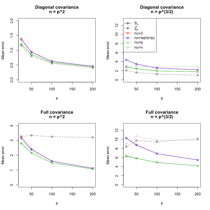
Figure 1: The risks for the Bayes estimator with $IW(\nu_{n},O_{p},K)$, the sample covariance $S_{n}$ and tapering estimator $\hat{\Sigma}_{k}$ under the spectral norm loss function. The true covariances were generated in diagonal setting (top row) and full covariance setting (bottom row). The number of the observation was chosen by either $n=p^{2}$ (left column) or $n=\lceil p^{3/2}\rceil$ (right column).

Figure 1 summarizes the simulation results for the spectral norm. Each point of the plot was calculated by

$$\frac{1}{100}\sum_{s=1}^{100}\|\Sigma_{0}-\widehat{\Sigma}_{n}^{(s)}\|$$

where $\widehat{\Sigma}_{n}^{(s)}$ is the estimate of the true covariance $\Sigma_{0}$ in $s$-th simulation. The first and second rows of Figure 1 show the results when the true covariance matrix is a diagonal and full covariance, respectively; the left and right columns are the results when $n=p^{2}$ and $n=\lceil p^{3/2}\rceil$, respectively.

The inverse-Wishart prior with $\nu_{n}=p$ and the sample covariance performed well in all cases. They are either the best or comparable to the best. When $n=\lceil p^{3/2}\rceil$, the truncated inverse-Wishart prior with $\nu_{n}=n$ is not minimax, and the simulation results show that it performed the worst or the second to the worst. The inverse-Wishart priors with $\nu_{n}=2$ and $\sqrt{n/p}$ are minimax, and thus their risks decrease as $n\longrightarrow\infty$ in all cases, but their performance are slightly worse than that with $\nu_{n}=p$. The tapering estimator $\hat{\Sigma}_{k}$ performed the best in diagonal settings because it gives zero to many of upper and lower diagonal elements or shrink them toward zero. However, in the full covariance settings, it performed the worst or close to the worst for the same reason.

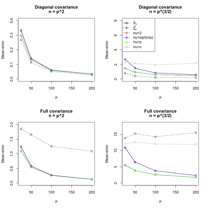
Figure 2: The risks for the Bayes estimator with $IW(\nu_{n},O_{p},K)$, the sample covariance $S_{n}$ and tapering estimator $\hat{\Sigma}_{k}$ under the squared Frobenius norm loss function. The true covariances were generated in diagonal setting (top row) and full covariance setting (bottom row). The number of the observation was chosen by either $n=p^{2}$ (left column) or $n=\lceil p^{3/2}\rceil$ (right column).

Figure 2 summarizes the simulation results for Frobenius norm. Each point of the plot was calculated by

$$\frac{1}{100}\sum_{s=1}^{100}\frac{1}{p}\|\Sigma_{0}-\widehat{\Sigma}_{n}^{(s)}\|_{F}^{2}$$

where $\widehat{\Sigma}_{n}^{(s)}$ is the estimate of the true covariance $\Sigma_{0}$ in $s$-th simulation. The results are quite similar to the spectral norm case.

For the square of log-determinant loss, we chose the maximum likelihood estimator (MLE) $\log\det S_{n}$ and the uniformly minimum variance unbiased estimator (UMVUE) for comparison. The UMVUE of $\log\det\Sigma$ is given by

$$\log\det S_{n}+p\log\left(\frac{n}{2}\right)-\sum_{j=0}^{p-1}\psi\left(\frac{n-k}{2}\right)$$

where $\psi$ is the digamma function which is defined by $\psi(x)=d/dz\log\Gamma(z)|_{z=x}$ where $\Gamma$ is the gamma function. See [1] for more details. We tried the same settings for inverse-Wishart prior as before. Note that for $n=p^{2}$ and $n=\lceil p^{3/2}\rceil$, the choices $\nu_{n}=2$ and $\sqrt{n/p}$ satisfy the sufficient condition in Theorem 3.7 while $\nu_{n}=p$ and $n$ do not. The posterior mean of the log-determinant for the inverse-Wishart prior is

$$\log\det\left(S_{n}+\frac{A_{n}}{n}\right)+p\log\left(\frac{n}{2}\right)-\sum_{j=0}^{p-1}\psi\left(\frac{n+\nu_{n}-k}{2}\right).$$

Thus, the UMVUE is the same as the Bayesian estimator using inverse-Wishart prior with $\nu_{n}=0$ and $A_{n}=O_{p}$, which satisfies the sufficient condition in Theorem 3.7.

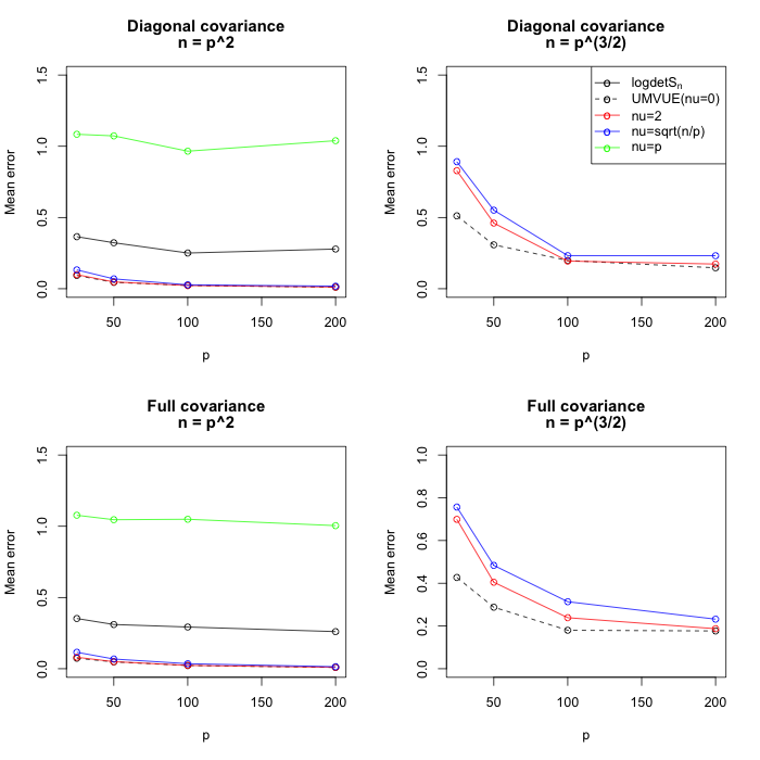
Figure 3: The squared log-determinant loss function plot. The true covariances were generated in diagonal setting (top row) and full covariance setting (bottom row). The number of the observation was chosen by either $n=p^{2}$ (left column) or $n=\lceil p^{3/2}\rceil$ (right column).

Figure 3 summarizes the simulation results for log-determinant. Each point of the plot was calculated by

$$\frac{1}{100}\sum_{s=1}^{100}(\log\det\Sigma_{0}-\widehat{\log\det\Sigma}_{n}^{(s)})^{2}$$

where $\widehat{\log\det\Sigma}_{n}^{(s)}$ is the estimate of $\log\det\Sigma$ in $s$-th simulation and $\Sigma_{0}$ is the true covariance. The top and bottom rows are for the diagonal and full true covariance cases, respectively; the left and right columns are for $n=p^{2}$ and $\lceil p^{3/2}\rceil$, respectively.

For the squared log-determinant loss, the inverse-Wishart priors with $\nu_{n}=2$ and $\sqrt{n/p}$ are minimax, while those with $\nu_{n}=p$ and $n$ are not. The UMVUE or the Bayes estimator of the the inverse-Wishart priors with $\nu_{n}=0$ performed the best in all cases. The inverse-Wishart priors with $\nu_{n}=2$ and $\sqrt{n/p}$ performed comparable to the UMVUE. Interestingly, the inverse-Wishart priors with $\nu_{n}=p$, which was the best under the spectral norm, performed worst in all cases. When $n=\lceil p^{3/2}\rceil$, the results for $\nu_{n}=p$ do not appear in the Figure 3 because of its large risk values. This signifies the fact that we need to choose different prior parameter for different loss function.

5 Discussion

In this paper, we develop a new framework for the Bayesian minimax theory, and introduce Bayesian minimax rate and P-loss convergence rate. The proposed decision theoretic framework gives an alternative way to distinguish the good priors from the inadequate ones and makes the definition of the minimax rate of the posterior clear. We obtain the Bayesian minimax rates for the normal covariance model under the various loss functions: spectral norm, the squared Frobenius norm, Bregman matrix divergence and squared log-determinant loss for large covariance estimation. We show that the inverse-Wishart prior or truncated inverse-Wishart prior attains the Bayesian minimax rate. The simulation results support the theory obtained.

Appendix A Basic properties of P-loss convergence rate

A frequentist minimax lower bound is defined as a lower bound of

$$\inf_{\hat{\Sigma}}\sup_{\Sigma_{0}\in\mathcal{C}_{p}}\mathbb{E}_{\Sigma_{0}}(d(\hat{\Sigma},\Sigma_{0}))$$

where $\hat{\Sigma}$ denotes an arbitrary estimator of $\Sigma_{0}$, and we say $r_{n}$ is the frequentist minimax rate for the class $\mathcal{C}_{p}$ and the space of the estimators of $\Sigma_{0}$, if

$$\inf_{\hat{\Sigma}}\sup_{\Sigma_{0}\in\mathcal{C}_{p}}\mathbb{E}_{\Sigma_{0}}(d(\hat{\Sigma},\Sigma_{0}))\asymp r_{n}.$$

Propositions A.1 and A.2 state two basic properties of P-loss convergence rate and the Bayesian minimax rate.

Proposition A.1

For any $\Sigma_{0}\in\mathcal{C}_{p}$, a P-loss convergence rate at $\Sigma_{0}$ is a posterior convergence rate at $\Sigma_{0}$.

• Suppose that the rate of the P-loss convergence rate at $\Sigma_{0}\in\mathcal{C}_{p}$ is $\epsilon_{n}$, i.e.,

  $$\mathbb{E}_{\Sigma_{0}}\mathbb{E}^{\pi}(d(\Sigma,\Sigma_{0})|{\bf X}_{n}) \asymp \epsilon_{n}.$$

  For a sequence $M_{n}\longrightarrow\infty$ and $\delta>0$,

  $$\mathbb{P}_{\Sigma_{0}}\left(\pi(d(\Sigma,\Sigma_{0})\geq M_{n}\epsilon_{n}\mid{\bf X}_{n})>\delta\right) \leq \mathbb{P}_{\Sigma_{0}}\left(\mathbb{E}^{\pi}(d(\Sigma,\Sigma_{0})\mid{\bf X}_{n})>\delta M_{n}\epsilon_{n}\right)$$

  $$\leq \frac{1}{\delta M_{n}\epsilon_{n}}\mathbb{E}_{\Sigma_{0}}\mathbb{E}^{\pi}(d(\Sigma,\Sigma_{0})\mid{\bf X}_{n})$$

  $$\longrightarrow 0,\quad\text{ as }n\to\infty.$$

  The first and second inequalities follow from the Markov inequality.

Proposition A.2

A frequentist minimax lower bound for $\Sigma_{0}$ is also a P-loss minimax lower bound for any loss function $d(\cdot,\Sigma_{0})$, i.e.,

$$\inf_{\pi\in\Pi_{n}}\sup_{\Sigma_{0}\in\mathcal{C}_{p}}\mathbb{E}_{\Sigma_{0}}\mathbb{E}^{\pi}(d(\Sigma,\Sigma_{0})\mid{\bf X}_{n}) \geq \inf_{\hat{\Sigma}}\sup_{\Sigma_{0}\in\mathcal{C}_{p}}\mathbb{E}_{\Sigma_{0}}(d(\hat{\Sigma},\Sigma_{0})),$$

where $\hat{\Sigma}$ denotes an arbitrary estimator of $\Sigma_{0}$.

• Note that the P-risk is always equal or larger than the posterior convergence rate by Markov’s inequality, and the frequentist minimax rate is a lower bound for the posterior convergence rate ([28]). Thus, the frequentist minimax rate is also a lower bound for the P-loss minimax rate.

Appendix B Proof of Theorem 3.1

We divide the proof of Theorem 3.1 into two parts: the lower bound part (Theorem B.1) and the upper bound part (Theorem B.2). For Theorem B.1, we have a quite strong result in sense that it holds even for $\tau_{1}$ and $\tau_{2}$ depending on $n$ and possibly $\tau_{1}\longrightarrow 0$ and $\tau_{2}\longrightarrow\infty$ as $n\longrightarrow\infty$.

Theorem B.1

Consider the model (1). For any positive constants $\tau_{1}<\tau_{2}$, for both fixed $p$ and $p\longrightarrow\infty$ as $n\longrightarrow\infty$,

$$\inf_{\pi\in\Pi_{n}}\sup_{\Sigma_{0}\in\mathcal{C}(\tau_{1},\tau_{2})}\mathbb{E}_{\Sigma_{0}}\mathbb{E}^{\pi}(\|\Sigma_{n}-\Sigma_{0}\|^{2}\mid{\bf X}_{n}) \geq c\cdot\tau_{2}^{2}\cdot\min\left(\frac{p}{n},1\right)$$

for all sufficiently large $n$ and some constant $c>0$.

Theorem B.2

Consider the model (1) and prior (3) with $\nu_{n}^{2}=O(np)$ and $\|A_{n}\|^{2}=O(np)$. For any positive constants $\tau_{1}<\tau_{2}$,

$$\sup_{\Sigma_{0}\in\mathcal{C}(\tau_{1},\tau_{2})}\mathbb{E}_{\Sigma_{0}}\mathbb{E}^{\pi}(\|\Sigma_{n}-\Sigma_{0}\|^{2}\mid{\bf X}_{n})\leq c\cdot\min\left(\frac{p}{n},1\right)$$

for all sufficiently large $n$ and some constant $c>0$.

B.1 Proof of Theorem B.1

Lemma B.3-B.5 are used to prove Theorem B.1. The proofs of Lemma B.3 and Lemma B.4 are straightforward, and they are omitted here.

Lemma B.3

Let $f_{i}$ be the density function of $p$-dimensional $N_{p}(0,\Sigma_{i}),i=0,1,2$. If $\Sigma_{1}^{-1}+\Sigma_{2}^{-2}-\Sigma_{0}^{-1}$ is a positive definite matrix,

$$\int_{\mathbb{R}^{p}}\frac{f_{1}f_{2}}{f_{0}}dx = [\text{det}(I_{p}-\Sigma_{0}^{-2}(\Sigma_{1}-\Sigma_{0})(\Sigma_{2}-\Sigma_{0}))]^{-1/2}.$$

Lemma B.4

Define $\mathcal{U}:=\{u\in\mathbb{R}^{p}:u_{i}=\pm 1/\sqrt{p},i=1,\cdots,p\}$. For any $u,v\sim Unif(\mathcal{U})$,

$$\langle u,v\rangle\stackrel{{\scriptstyle d}}{{\equiv}}2B/p-1$$

where $B\sim Bin(p,1/2)$.

Lemma B.5

Let $P_{0},P_{1}\in\mathcal{P}$ where $\mathcal{P}$ is a set of all probability measures on $\mathcal{X}$ and let $f_{0}$ and $f_{1}$ be their density functions, respectively. Define $\xi=\xi(P_{0},P_{1}):=\int_{\mathcal{X}}f_{1}^{2}/f_{0}dx$ and set $\theta_{i}=\theta(P_{i}),i=0,1$, where $\theta$ is a functional defined on $\mathcal{P}$. Then

$$\inf_{\delta}\max\{\mathbb{E}_{0}(\delta-\theta_{0})^{2},\mathbb{E}_{1}(\delta-\theta_{1})^{2}\}\geq\frac{(\theta_{1}-\theta_{0})^{2}}{(1+\xi^{1/2})^{2}},$$

where $\delta$ denotes any estimator of $\theta$ and $\mathbb{E}_{i}$ represents the expectation with respect to $P_{i}$, $i=0,1$.

• For given estimator $\delta$ which satisfies $R(\delta,\theta_{0})=\mathbb{E}|\delta(X)-\theta|^{2}\leq\epsilon^{2}$, we have

  $$R(\delta,\theta_{1})\geq(|\theta_{1}-\theta_{0}|-\epsilon\xi^{1/2})^{2}$$

  by [8]. Choose $\epsilon=|\theta_{1}-\theta_{0}|/(1+\xi^{1/2})$ so that

  $$\epsilon^{2} = (|\theta_{1}-\theta_{0}|-\epsilon\xi^{1/2})^{2}.$$

  If $\mathbb{E}_{0}(\delta-\theta_{0})^{2}\leq\epsilon^{2}$, we have

  $$\max\{\mathbb{E}_{0}(\delta-\theta_{0})^{2},\mathbb{E}_{1}(\delta-\theta_{1})^{2}\}\geq\mathbb{E}_{1}(\delta-\theta_{1})^{2}\geq\epsilon^{2}=\frac{(\theta_{1}-\theta_{0})^{2}}{(1+\xi^{1/2})^{2}}$$

  If $\mathbb{E}_{0}(\delta-\theta_{0})^{2}\geq\epsilon^{2}$, we have

  $$\max\{\mathbb{E}_{0}(\delta-\theta_{0})^{2},\mathbb{E}_{1}(\delta-\theta_{1})^{2}\}\geq\mathbb{E}_{0}(\delta-\theta_{0})^{2}\geq\epsilon^{2}=\frac{(\theta_{1}-\theta_{0})^{2}}{(1+\xi^{1/2})^{2}}.$$

  Hence,

  $$\inf_{\delta}\max\{\mathbb{E}_{0}(\delta-\theta_{0})^{2},\mathbb{E}_{1}(\delta-\theta_{1})^{2}\} \geq \frac{(\theta_{1}-\theta_{0})^{2}}{(1+\xi^{\frac{1}{2}})^{2}}.$$

• It suffices to show that

  $$\inf_{\hat{\Sigma}_{n}}\sup_{\Sigma_{0}\in\mathcal{C}(\tau_{1},\tau_{2})}\mathbb{E}_{\Sigma_{0}}\|\hat{\Sigma}_{n}-\Sigma_{0}\|^{2} \geq c^{\prime}\cdot\tau_{2}^{2}\cdot\min\left(\frac{p}{n},1\right)$$

  for some constant $c^{\prime}>0$ because by the Jensen’s inequality,

  $$\inf_{\pi\in\Pi_{n}}\sup_{\Sigma_{0}\in\mathcal{C}(\tau_{1},\tau_{2})}\mathbb{E}_{\Sigma_{0}}\mathbb{E}^{\pi}(\|\Sigma_{n}-\Sigma_{0}\|^{2}\mid{\bf X}_{n}) \geq \inf_{\pi\in\Pi_{n}}\sup_{\Sigma_{0}\in\mathcal{C}(\tau_{1},\tau_{2})}\mathbb{E}_{\Sigma_{0}}\|\tilde{\Sigma}_{n}-\Sigma_{0}\|^{2}$$

  $$\geq \inf_{\hat{\Sigma}_{n}}\sup_{\Sigma_{0}\in\mathcal{C}(\tau_{1},\tau_{2})}\mathbb{E}_{\Sigma_{0}}\|\hat{\Sigma}_{n}-\Sigma_{0}\|^{2},$$

  where $\tilde{\Sigma}_{n}:=\mathbb{E}^{\pi}(\Sigma_{n}\mid{\bf X}_{n})$. Assume $n\geq p$ and define

  $$\mathcal{U} := \Big{\{}u=(u_{1},\ldots,u_{p})\in\mathbb{R}^{p}:u_{i}=\pm 1/\sqrt{p},i=1,\cdots,p\Big{\}},$$

  $$\Theta := \Big{\{}\Sigma\in\mathbb{R}^{p\times p}:\Sigma=\frac{\tau_{2}}{1+\epsilon}\big{[}I_{p}+\epsilon uu^{T}\big{]},u\in\mathcal{U}\Big{\}}$$

  with $\epsilon=c\sqrt{p/n}\leq 1$ for some small $c>0$ satisfying $\epsilon\leq\tau_{2}/\tau_{1}-1$. Let $P_{0}^{n}=N(0,2^{-1}\tau_{2}I_{p})^{n},P_{1}^{n}=2^{-p}\sum_{\Sigma\in\Theta}N(0,\Sigma)^{n}$ and let $f_{0}^{n}$ and $f_{1}^{n}$ be their density functions, respectively. Note that $\|\Sigma\|=\tau_{2}$ and $\lambda_{min}(\Sigma)=(1+\epsilon)^{-1}\tau_{2}\geq\tau_{1}$ for any $\Sigma\in\Theta$, thus $\Theta\subset\mathcal{C}(\tau_{1},\tau_{2})$ for some small $c>0$. By the above Lemma B.5,

  $$\inf_{\hat{\Sigma}_{n}}\sup_{\Sigma_{0}\in\mathcal{C}(\tau_{1},\tau_{2})}\mathbb{E}_{\Sigma_{0}}\|\hat{\Sigma}_{n}-\Sigma_{0}\|^{2} \geq \inf_{\hat{\Sigma}_{n}}\sup_{\Sigma_{0}\in\mathcal{C}(\tau_{1},\tau_{2})}\mathbb{E}_{\Sigma_{0}}(\|\hat{\Sigma}_{n}\|-\|\Sigma_{0}\|)^{2}$$

  $$\geq \inf_{\delta}\sup_{\Sigma_{0}\in\mathcal{C}(\tau_{1},\tau_{2})}\mathbb{E}_{\Sigma_{0}}(\delta-\|\Sigma_{0}\|)^{2}$$

  $$\geq \underset{\delta}{\inf}\underset{\Sigma_{0}\in\{2^{-1}\tau_{2}I_{p}\}\cup\Theta}{\max}\mathbb{E}_{\Sigma_{0}}(\delta-\|\Sigma_{0}\|)^{2}$$

  $$\geq \underset{\delta}{\inf}\max(\mathbb{E}_{f_{0}^{n}}(\delta-(1+\epsilon)^{-1}\tau_{2})^{2},\mathbb{E}_{f_{1}^{n}}(\delta-\tau_{2})^{2})$$

  $$\geq \frac{\tau_{2}^{2}\epsilon^{2}}{4(1+\xi^{1/2})^{2}},$$

  where $\delta$ denotes any estimator of $\|\Sigma_{0}\|$ and $\xi:=\int(f_{1}^{n})^{2}/f_{0}^{n}$. The fourth inequality follows from

  $$\inf_{\delta}\max_{\Sigma\in\Theta}\mathbb{E}_{f_{\Sigma}}(\delta-\|\Sigma\|)^{2} = \inf_{\delta}\max_{\Sigma\in\Theta}\int(\delta(x)-\tau_{2})^{2}f_{\Sigma}^{n}(x)dx$$

  $$\geq \inf_{\delta}\frac{1}{2^{p}}\sum_{\Sigma\in\Theta}\int(\delta(x)-\tau_{2})^{2}f_{\Sigma}^{n}(x)dx$$

  $$= \inf_{\delta}\int(\delta(x)-\tau_{2})^{2}f_{1}^{n}(x)dx$$

  $$= \inf_{\delta}\mathbb{E}_{f_{1}^{n}}(\delta-\tau_{2})^{2}$$

  where $f_{\Sigma}^{n}$ is the density function of $N(0,\Sigma)^{n}$. Now we calculate $\xi$.

  $$\xi = \int\frac{(f_{1}^{n})^{2}}{f_{0}^{n}}$$

  $$= \int\frac{(2^{-p}\sum_{\Sigma\in\Theta}f_{\Sigma}^{n})^{2}}{f_{0}^{n}}$$

  $$= \frac{1}{2^{2p}}\sum_{\Sigma_{1},\Sigma_{2}\in\Theta}\int\frac{f_{\Sigma_{1}}^{n}f_{\Sigma_{2}}^{n}}{f_{0}^{n}}$$

  $$= \frac{1}{2^{2p}}\sum_{\Sigma_{1},\Sigma_{2}\in\Theta}\left(\int\frac{f_{\Sigma_{1}}f_{\Sigma_{2}}}{f_{0}}\right)^{n}$$

  $$= \frac{1}{2^{2p}}\sum_{u,v\in\mathcal{U}}\det[(I_{p}-\epsilon^{2}uu^{T}vv^{T})]^{-n/2}$$

  $$= \frac{1}{2^{2p}}\sum_{u,v\in\mathcal{U}}(1-\epsilon^{2}(u^{T}v)^{2})^{-n/2}$$

  $$= \mathbb{E}(1-\epsilon^{2}\langle u,v\rangle^{2})^{-n/2}$$

  $$\leq \mathbb{E}(\exp(2n\epsilon^{2}\langle u,v\rangle^{2})),$$

  where $u,v\sim Unif(\mathcal{U})$. The fifth equality is derived from Lemma B.3. We will show that $\xi\leq C$ for some constant $C>0$ for all sufficiently large $n$. If $p$ does not grow to infinity, i.e., $p\leq C$ for some constant $C>0$, the last term bounded above easily, $\mathbb{E}(\exp(2n\epsilon^{2}\langle u,v\rangle^{2}))\leq\exp(2c^{2}p)\leq\exp(2c^{2}C)$. If $p$ tends to infinity, by the Lemma B.4, note that $\sqrt{p}\langle u,v\rangle\stackrel{{\scriptstyle d}}{{\equiv}}\sqrt{p}(2B/p-1)\overset{d}{\longrightarrow}N(0,1)$ as $n\longrightarrow\infty$ where $B\sim Bin(p,1/2)$. Note also that we have

  $$\mathbb{E}\left(\exp\left[cp\left(\frac{2}{p}B-1\right)^{2}\right]\right) \longrightarrow \mathbb{E}(\exp(cZ^{2}))=\frac{1}{\sqrt{1-2c}}$$

  by Theorem 1 of [33] for $0<c<1/2,~{}Z\sim N(0,1)$. In our setting, consider $F_{p}$ as the distribution function of $p(2B/p-1)^{2}$. Thus, we get the followings by taking $\epsilon=c\sqrt{p/n}$ for some small $c>0$ such that $2c<1/2$,

  $$\xi \leq \mathbb{E}\left(\exp\left[2cp\left(\frac{2}{p}B-1\right)^{2}\right]\right)$$

  $$\longrightarrow \frac{1}{\sqrt{1-4c}},$$

  as $n\longrightarrow\infty$. Hence, we have

  $$\underset{\hat{\Sigma}_{n}}{\inf}\underset{\Sigma_{0}\in\mathcal{C}(\tau_{1},\tau_{2})}{\sup}\mathbb{E}_{\Sigma_{0}}\|\hat{\Sigma}_{n}-\Sigma_{0}\|^{2}\geq\frac{\tau_{2}^{2}\epsilon^{2}}{4(1+\xi^{1/2})^{2}}\geq c^{\prime}\cdot\tau_{2}^{2}\cdot\frac{p}{n}$$

  for some $c^{\prime}>0$ which proves the lower bound when $n\geq p$.

  Now, assume $n<p$ and define

  $$\mathcal{U}_{n} := \Big{\{}u\in\mathbb{R}^{n}:u_{i}=\pm\frac{1}{\sqrt{n}},i=1,\ldots,n\Big{\}}$$

  $$\Theta := \left\{\Sigma=\begin{pmatrix}\Sigma_{n}&0\\ 0&I_{p-n}\end{pmatrix}:\Sigma_{n}=\frac{\tau_{2}}{1+\epsilon}\big{[}I_{n}+\epsilon uu^{T}\big{]},u\in\mathcal{U}_{n}\right\}.$$

  Earlier result shows that

  $$\inf_{\hat{\Sigma}_{n}}\sup_{\Sigma_{0}\in\mathcal{C}(\tau_{1},\tau_{2})}\mathbb{E}\|\hat{\Sigma}_{n}-\Sigma_{0}\|^{2} \geq \inf_{\hat{\Sigma}_{n}}\max_{\Sigma_{0}\in\Theta}\mathbb{E}\|\hat{\Sigma}_{n}-\Sigma_{0}\|^{2}$$

  $$\geq c^{\prime}\cdot\tau_{2}^{2}\cdot\frac{n}{n}=c^{\prime}\cdot\tau_{2}^{2}$$

  for some $c^{\prime}>0$.

B.2 Proof of Theorem B.2

Lemma B.6

Let $\Omega_{n}\sim W_{p}(\nu_{n},\nu_{n}^{-1}A_{n})$ with $\nu_{n}>p$ and positive definite matrix $A_{n}$, for all $n\geq 1$ and $\|A_{n}\|\leq\tau_{n}$ for all sufficiently large $n$. Then, there exist positive constants $c_{1}$ and $c_{2}$ such that

$$\mathbb{P}(\|\Omega_{n}-A_{n}\|\geq x) \leq 5^{p}\left(e^{-c_{1}\nu_{n}x^{2}/\tau_{n}^{2}}+e^{-c_{2}\nu_{n}x/\tau_{n}}\right)$$

for all $x>0$.

• There exist $v_{j}$ with $\|v_{j}\|_{2}=1$ for $j=1,\ldots,5^{p}$, such that

  $$\|A\| \leq 4\cdot\sup_{j\leq 5^{p}}|v_{j}^{T}Av_{j}|$$

  for any $p\times p$ symmetric matrix $A$ (Page 2141 of [11]). Thus, we have

  $$\mathbb{P}(\|\Omega_{n}-A_{n}\|\geq x) \leq \mathbb{P}(\|A_{n}\|\|A_{n}^{-1/2}\Omega_{n}A_{n}^{-1/2}-I_{p}\|\geq x)$$

  $$\leq \mathbb{P}(\|A_{n}^{-1/2}\Omega_{n}A_{n}^{-1/2}-I_{p}\|\geq x/\tau_{n})$$

  $$\leq \mathbb{P}\left(4\cdot\sup_{j\leq 5^{p}}|v_{j}^{T}(A_{n}^{-1/2}\Omega_{n}A_{n}^{-1/2}-I_{p})v_{j}|\geq x/\tau_{n}\right)$$

  $$\leq 5^{p}\sup_{j\leq 5^{p}}\pi\left(|v_{j}^{T}(A_{n}^{-1/2}\Omega_{n}A_{n}^{-1/2}-I_{p})v_{j}|\geq x/(4\tau_{n})\right)$$

  $$\leq 5^{p}\left(e^{-c_{1}\nu_{n}x^{2}/\tau_{n}^{2}}+e^{-c_{2}\nu_{n}x/\tau_{n}}\right).$$

  The last inequality follows from Lemma 2.4 and Theorem 3.2 of [39] because $A_{n}^{-1/2}\Omega_{n}A_{n}^{-1/2}\sim W_{p}(\nu_{n},\nu_{n}^{-1}I_{p})$.

Lemma B.7

Let $\Omega_{n}\sim W_{p}(\nu_{n},\nu_{n}^{-1}I_{p})$ with $c\nu_{n}\geq p$ for some constant $0<c<1$. Then ,

$$\pi(\lambda_{max}(\Omega_{n})\geq c_{1}) \leq 2e^{-\nu_{n}/2},$$

$$\pi(\lambda_{min}(\Omega_{n})\leq c_{2}) \leq 2e^{-\nu_{n}(1-\sqrt{p/\nu_{n}})^{2}/8}$$

for any constant $c_{1}\geq(2+\sqrt{p/\nu_{n}})^{2}$ and $0<c_{2}\leq(1-\sqrt{p/\nu_{n}})^{2}/4$.

• It follows from Corollary 5.35 in [20],

  $$\pi(\lambda_{max}(\Omega_{n})^{1/2}\geq 1+\sqrt{p/\nu_{n}}+t/\sqrt{\nu_{n}}) \leq 2e^{-t^{2}/2},$$ (5)

  $$\pi(\lambda_{min}(\Omega_{n})^{1/2}\leq 1-\sqrt{p/\nu_{n}}-t/\sqrt{\nu_{n}}) \leq 2e^{-t^{2}/2}$$ (6)

  for any $t\geq 0$. If we choose $t=\sqrt{\nu_{n}}$ for (5), it gives the first inequality

  $$\pi(\lambda_{max}(\Omega_{n})\geq(2+\sqrt{p/\nu_{n}})^{2}) \leq 2e^{-\nu_{n}/2}.$$

  If we choose $t=\sqrt{\nu_{n}}(1-\sqrt{p/\nu_{n}}-(1-\sqrt{p/\nu_{n}})/2)>0$ for (6), it gives the second inequality

  $$\pi(\lambda_{min}(\Omega_{n})\leq(1-\sqrt{p/\nu_{n}})^{2}/4) \leq 2e^{-\nu_{n}(1-\sqrt{p/\nu_{n}}-(1-\sqrt{p/\nu_{n}})/2)^{2}/2}$$

  $$\leq 2e^{-\nu_{n}(1-\sqrt{p/\nu_{n}})^{2}/8}.$$

• We prove the upper bound for $p\leq n/2$ case first. Note that

  $$\mathbb{E}_{\Sigma_{0}}\mathbb{E}^{\pi}(\|\Sigma_{n}-\Sigma_{0}\|\mid{\bf X}_{n})$$ (7)

  $$\leq \mathbb{E}_{\Sigma_{0}}\mathbb{E}^{\pi}(\|\Sigma_{n}-\breve{\Sigma}_{n}\|\mid{\bf X}_{n})+\mathbb{E}_{\Sigma_{0}}\|\breve{\Sigma}_{n}-\Sigma_{0}\|,$$

  where $\breve{\Sigma}_{n}:=(nS_{n}+A_{n})/(n+\nu_{n})$. Consider the first term of right hand side (RHS) of (7).

  $$\mathbb{E}_{\Sigma_{0}}\mathbb{E}^{\pi}(\|\Sigma_{n}-\breve{\Sigma}_{n}\|\mid{\bf X}_{n})$$ (8)

  $$= \mathbb{E}_{\Sigma_{0}}\left[\mathbb{E}^{\pi}(\|\Sigma_{n}-\breve{\Sigma}_{n}\|\mid{\bf X}_{n})I(\|\breve{\Sigma}_{n}\|\leq C_{1}\text{ and }\|\breve{\Sigma}_{n}^{-1}\|\leq C_{2})\right]$$

  $$+ \mathbb{E}_{\Sigma_{0}}\left[\mathbb{E}^{\pi}(\|\Sigma_{n}-\breve{\Sigma}_{n}\|\mid{\bf X}_{n})I(\|\breve{\Sigma}_{n}\|>C_{1}\text{ or }\|\breve{\Sigma}_{n}^{-1}\|>C_{2})\right]$$ (9)

  for any constant $C_{1}$ and $C_{2}$. The integrand of (8) is bounded by

  $$\mathbb{E}^{\pi}(\|\Sigma_{n}-\breve{\Sigma}_{n}\|\mid{\bf X}_{n})I(\|\breve{\Sigma}_{n}\|\leq C_{1}\text{ and }\|\breve{\Sigma}_{n}^{-1}\|\leq C_{2})$$

  $$\leq \mathbb{E}^{\pi}(\|\Sigma_{n}\|\|\Sigma_{n}^{-1}\breve{\Sigma}_{n}-I_{p}\|\mid{\bf X}_{n})I(\|\breve{\Sigma}_{n}\|\leq C_{1}\text{ and }\|\breve{\Sigma}_{n}^{-1}\|\leq C_{2})$$

  $$\leq \mathbb{E}^{\pi}(\|\Sigma_{n}\|\|\breve{\Sigma}_{n}^{-1/2}\|\|\breve{\Sigma}_{n}^{1/2}\Sigma_{n}^{-1}\breve{\Sigma}_{n}^{1/2}-I_{p}\|\|\breve{\Sigma}_{n}^{1/2}\|\mid{\bf X}_{n})I(\|\breve{\Sigma}_{n}\|\leq C_{1}\text{ and }\|\breve{\Sigma}_{n}^{-1}\|\leq C_{2})$$

  $$\leq \sqrt{C_{1}C_{2}}\cdot\mathbb{E}^{\pi}(\|\Sigma_{n}\|\|\breve{\Sigma}_{n}^{1/2}\Sigma_{n}^{-1}\breve{\Sigma}_{n}^{1/2}-I_{p}\|\mid{\bf X}_{n})I(\|\breve{\Sigma}_{n}\|\leq C_{1}\text{ and }\|\breve{\Sigma}_{n}^{-1}\|\leq C_{2})$$

  $$\leq \sqrt{C_{1}C_{2}}\cdot\left[\mathbb{E}^{\pi}(\|\Sigma_{n}\|^{2}\mid{\bf X}_{n})I(\|\breve{\Sigma}_{n}\|\leq C_{1}\text{ and }\|\breve{\Sigma}_{n}^{-1}\|\leq C_{2})\right]^{1/2}$$

  $$\times \left[\mathbb{E}^{\pi}(\|\breve{\Sigma}_{n}^{1/2}\Sigma_{n}^{-1}\breve{\Sigma}_{n}^{1/2}-I_{p}\|^{2}\mid{\bf X}_{n})\right]^{1/2}.$$

  To show that

  $$\mathbb{E}_{\Sigma_{0}}\left[\mathbb{E}^{\pi}(\|\Sigma_{n}-\breve{\Sigma}_{n}\|\mid{\bf X}_{n})I(\|\breve{\Sigma}_{n}\|\leq C_{1}\text{ and }\|\breve{\Sigma}_{n}^{-1}\|\leq C_{2})\right] \lesssim \sqrt{p/n},$$

  it suffices to prove that $\mathbb{E}^{\pi}(\|\breve{\Sigma}_{n}^{1/2}\Sigma_{n}^{-1}\breve{\Sigma}_{n}^{1/2}-I_{p}\|^{2}\mid{\bf X}_{n})\lesssim p/n$ and $\mathbb{E}^{\pi}(\|\Sigma_{n}\|^{2}\mid{\bf X}_{n})I(\|\breve{\Sigma}_{n}\|\leq C_{1}\text{ and }\|\breve{\Sigma}_{n}^{-1}\|\leq C_{2})=O(1)$. Note that

  $$\mathbb{E}^{\pi}(\|\breve{\Sigma}_{n}^{1/2}\Sigma_{n}^{-1}\breve{\Sigma}_{n}^{1/2}-I_{p}\|^{2}\mid{\bf X}_{n})$$ (10)

  $$\leq \int_{x}^{\infty}\pi(\|\breve{\Sigma}_{n}^{1/2}\Sigma_{n}^{-1}\breve{\Sigma}_{n}^{1/2}-I_{p}\|^{2}\geq u\mid{\bf X}_{n})du+x$$

  $$\leq \int_{x}^{\infty}5^{p}\left(e^{-C_{3}(n+\nu_{n})u}+e^{-C_{4}(n+\nu_{n})\sqrt{u}}\right)du+x$$

  $$\leq \frac{5^{p}e^{-C_{3}(n+\nu_{n})x}}{C_{3}(n+\nu_{n})}+\frac{5^{p}\cdot 2\sqrt{x}e^{-C_{4}(n+\nu_{n})\sqrt{x}}}{C_{4}(n+\nu_{n})}+\frac{5^{p}\cdot 2e^{-C_{4}(n+\nu_{n})\sqrt{x}}}{C_{4}^{2}(n+\nu_{n})^{2}}+x$$

  for any $x>0$ and some positive constants $C_{3}$ and $C_{4}$ by Lemma B.6. If we choose $x=C_{5}\cdot p/n$ for some large $C_{5}>0$, the rate of (10) is $p/n$. Note that

  $$\mathbb{E}^{\pi}\left(\|\Sigma_{n}\|^{2}\mid{\bf X}_{n}\right) \leq \mathbb{E}^{\pi}\left(\|\Sigma_{n}\|^{2}I(\|\Sigma_{n}\|>C_{6})\mid{\bf X}_{n}\right)+C_{6}^{2}$$

  $$\leq \left[\mathbb{E}^{\pi}\left(\|\Sigma_{n}\|^{4}\mid{\bf X}_{n}\right)\right]^{1/2}\left[\pi\left(\|\Sigma_{n}\|>C_{6}\mid{\bf X}_{n}\right)\right]^{1/2}+C_{6}^{2},$$

  by Hölder’s inequality. One can easily show that $\mathbb{E}^{\pi}(\|\Sigma_{n}\|^{4}\mid{\bf X}_{n})$ is bounded above by $p^{5}$ up to some constant factor because $\|\Sigma_{n}\|\leq tr(\Sigma_{n})$ and $\mathbb{E}^{\pi}(tr(\Sigma_{n})^{4}\mid{\bf X}_{n})I(\|\breve{\Sigma}_{n}\|\leq C_{1}\text{ and }\|\breve{\Sigma}_{n}^{-1}\|\leq C_{2})\lesssim p^{4}$. Also note that

  $$\pi\left(\|\Sigma_{n}\|>C_{6}\mid{\bf X}_{n}\right) = \pi\left(\lambda_{min}(\Sigma_{n}^{-1})<C_{6}^{-1}\mid{\bf X}_{n}\right)$$

  $$\leq \pi\left(\lambda_{min}(\breve{\Sigma}_{n}^{1/2}\Sigma_{n}^{-1}\breve{\Sigma}_{n}^{1/2})<\|\breve{\Sigma}_{n}\|C_{6}^{-1}\mid{\bf X}_{n})\right)$$

  $$\leq \pi\left(\lambda_{min}(\breve{\Sigma}_{n}^{1/2}\Sigma_{n}^{-1}\breve{\Sigma}_{n}^{1/2})<C_{1}C_{6}^{-1}\mid{\bf X}_{n})\right)$$

  $$\leq 2e^{-(n+\nu_{n})(1-\sqrt{p/(n+\nu_{n})})^{2}/8}$$

  for some constant $C_{6}\geq C_{1}\cdot 4(1-\sqrt{1/2})^{-2}$ by Lemma B.7. Thus, we have shown that the rate of (8) is smaller than $\sqrt{p/n}$.

  Now, we show that the rate of (9) is smaller than $\sqrt{p/n}$. Note that (9) is bounded by

  $$\mathbb{E}_{\Sigma_{0}}\left[\mathbb{E}^{\pi}(\|\Sigma_{n}-\breve{\Sigma}_{n}\|\mid{\bf X}_{n})I(\|\breve{\Sigma}_{n}\|>C_{1}\text{ or }\|\breve{\Sigma}_{n}^{-1}\|>C_{2})\right]$$

  $$\leq \mathbb{E}_{\Sigma_{0}}\left[\left(\mathbb{E}^{\pi}(\|\Sigma_{n}\|\mid{\bf X}_{n})+\|\breve{\Sigma}_{n}\|\right)I(\|\breve{\Sigma}_{n}\|>C_{1}\text{ or }\|\breve{\Sigma}_{n}^{-1}\|>C_{2})\right]$$

  $$\leq \mathbb{E}_{\Sigma_{0}}\left[\mathbb{E}^{\pi}(\|\Sigma_{n}\|\mid{\bf X}_{n})I(\|\breve{\Sigma}_{n}\|>C_{1})\right]+\mathbb{E}_{\Sigma_{0}}\left[\mathbb{E}^{\pi}(\|\Sigma_{n}\|\mid{\bf X}_{n})I(\|\breve{\Sigma}_{n}^{-1}\|>C_{2})\right]$$

  $$+ \mathbb{E}_{\Sigma_{0}}\left[\|\breve{\Sigma}_{n}\|I(\|\breve{\Sigma}_{n}\|>C_{1})\right]+\mathbb{E}_{\Sigma_{0}}\left[\|\breve{\Sigma}_{n}\|I(\|\breve{\Sigma}_{n}^{-1}\|>C_{2})\right]$$

  Since $\breve{\Sigma}_{n}=(nS_{n}+A_{n})/(n+\nu_{n})$ and $\Sigma_{0}\in\mathcal{C}(\tau_{1},\tau_{2})$, we have

  $$\mathbb{P}_{\Sigma_{0}}(\|\breve{\Sigma}_{n}\|>C_{1}) \leq \mathbb{P}_{\Sigma_{0}}\left(\|S_{n}\|+\frac{\|A_{n}\|}{n+\nu_{n}}>C_{1}\right)$$ (11)

  $$= \mathbb{P}_{\Sigma_{0}}\left(\|S_{n}\|>C_{1}-\frac{\|A_{n}\|}{n+\nu_{n}}\right)$$

  $$\leq \mathbb{P}_{\Sigma_{0}}\left(\|\bar{S}_{n}\|>\tau^{-1}_{2}\left(C_{1}-\frac{\|A_{n}\|}{n+\nu_{n}}\right)\right)$$

  where $\bar{S}_{n}:=\Sigma_{0}^{-1/2}S_{n}\Sigma_{0}^{-1/2}\sim W_{p}(n,n^{-1}I_{p})$. Then, (11) is bounded by $2e^{-n/2}$ for some constant $C_{1}>0$ by Lemma B.7. Similarly, for some constant $C_{2}$,

  $$\mathbb{P}_{\Sigma_{0}}(\|\breve{\Sigma}_{n}^{-1}\|>C_{2}) \leq \mathbb{P}_{\Sigma_{0}}\left(\frac{n+\nu_{n}}{n}\cdot\|S_{n}^{-1}\|>C_{2}\right)$$

  $$= \mathbb{P}_{\Sigma_{0}}\left(\lambda_{min}(S_{n})<\left(1+\frac{\nu_{n}}{n}\right)C_{2}^{-1}\right)$$

  $$\leq \mathbb{P}_{\Sigma_{0}}\left(\lambda_{min}(\bar{S}_{n})<\tau_{1}^{-1}\left(1+\frac{\nu_{n}}{n}\right)C_{2}^{-1}\right)$$

  $$\leq 2e^{-n(1-\sqrt{p/n})^{2}/8},$$

  by Lemma B.7. It is easy to show that

  $$\mathbb{E}^{\pi}(\|\Sigma_{n}\|\mid{\bf X}_{n}) \leq \frac{(n+\nu_{n})p}{n+\nu_{n}-p-1}\|\breve{\Sigma}_{n}\|$$

  and

  $$\mathbb{E}_{\Sigma_{0}}\left[\|\breve{\Sigma}_{n}\|I(\|\breve{\Sigma}_{n}\|>C_{1})\right] = \int_{0}^{\infty}\mathbb{P}_{\Sigma_{0}}\left[\|\breve{\Sigma}_{n}\|I(\|\breve{\Sigma}_{n}\|>C_{1})\geq u\right]du$$

  $$= \int_{C_{1}}^{\infty}\mathbb{P}_{\Sigma_{0}}(\|\breve{\Sigma}_{n}\|\geq u)du$$

  $$\leq \int_{C_{1}}^{\infty}\mathbb{P}_{\Sigma_{0}}\left(\|\bar{S}_{n}\|\geq\tau^{-1}_{2}\left(u-\frac{\|A_{n}\|}{n+\nu_{n}}\right)\right)du.$$

  By applying $t=\sqrt{n}(\sqrt{\tau^{-1}_{2}(u-\|A_{n}\|/(n+\nu_{n}))}-1-\sqrt{p/n})$ to the tail inequality (5), we have

  $$\int_{C_{1}}^{\infty}\mathbb{P}_{\Sigma_{0}}\left(\|\bar{S}_{n}\|\geq\tau^{-1}_{2}\left(u-\frac{\|A_{n}\|}{n+\nu_{n}}\right)\right)du$$

  $$\leq \int_{C_{1}}^{\infty}2e^{-n(\sqrt{\tau^{-1}_{2}(u-\|A_{n}\|/(n+\nu_{n}))}-1-\sqrt{p/n})^{2}/2}du$$

  $$\leq \int_{C_{1}}^{\infty}2e^{-n\sqrt{u}C_{7}/2}du$$

  $$\leq \frac{\sqrt{C_{1}}}{C_{7}n}e^{-\sqrt{C_{1}}C_{7}n/2}+\frac{1}{2C_{7}^{2}n^{2}}e^{-\sqrt{C_{1}}C_{7}n/2}$$

  for some constant $C_{7}>0$. Also note that

  $$\mathbb{E}_{\Sigma_{0}}\left[\|\breve{\Sigma}_{n}\|I(\|\breve{\Sigma}_{n}^{-1}\|>C_{2})\right] \leq \left[\mathbb{E}_{\Sigma_{0}}\|\breve{\Sigma}_{n}\|^{2}\cdot\mathbb{P}_{\Sigma_{0}}\left(\|\breve{\Sigma}_{n}^{-1}\|>C_{2}\right)\right]^{1/2}$$

  $$\leq \left[\mathbb{E}_{\Sigma_{0}}\|\breve{\Sigma}_{n}\|^{2}\cdot 2e^{-n(1-\sqrt{p/n})^{2}/8}\right]^{1/2}$$

  and

  $$\mathbb{E}_{\Sigma_{0}}\|\breve{\Sigma}_{n}\|^{2} \leq 2\frac{\|A_{n}\|^{2}}{(n+\nu_{n})^{2}}+2\mathbb{E}_{\Sigma_{0}}\|S_{n}\|^{2}$$

  $$\leq 2\sup_{n}\frac{\|A_{n}\|^{2}}{(n+\nu_{n})^{2}}+\int_{0}^{\infty}\mathbb{P}_{\Sigma_{0}}\left(\|S_{n}\|^{2}\geq u\right)du$$

  $$\leq C_{8}+\int_{C_{9}}^{\infty}\mathbb{P}_{\Sigma_{0}}\left(\|\bar{S}_{n}\|\geq\sqrt{u}/\tau_{2}\right)du$$

  $$\leq C_{8}+\int_{C_{9}}^{\infty}2e^{-n(u^{1/4}/\sqrt{\tau_{2}}-1-\sqrt{p/n})^{2}/2}du$$

  $$\leq C_{8}+\int_{C_{9}}^{\infty}2e^{-nC_{10}\sqrt{u}/2}du$$

  for some positive constants $C_{8},C_{9}$ and $C_{10}$ by applying the tail inequality (5). Thus, we have shown that the rate of (9) is faster than $\sqrt{p/n}$.

For the second term of RHS of (7), note that

$$\mathbb{E}_{\Sigma_{0}}\|\breve{\Sigma}_{n}-\Sigma_{0}\| \leq \mathbb{E}_{\Sigma_{0}}\left\|S_{n}-\Sigma_{0}\right\|+\left(\frac{\nu_{n}}{n+\nu_{n}}\right)\mathbb{E}_{\Sigma_{0}}\|S_{n}\|+\frac{\|A_{n}\|}{n+\nu_{n}}.$$

Since $\nu_{n}^{2}=O(np)$ and $\|A_{n}\|^{2}=O(np)$, it is trivial that $\nu_{n}/(n+\nu_{n})\lesssim\sqrt{p/n}$ and $\|A_{n}\|/(n+\nu_{n})\lesssim\sqrt{p/n}$. One can show that $\mathbb{E}_{\Sigma_{0}}\|S_{n}-\Sigma_{0}\|\leq\mathbb{E}_{\Sigma_{0}}\|\bar{S}_{n}-I_{p}\|\cdot\|\Sigma_{0}\|\lesssim\sqrt{p/n}$ by Lemma B.6. Furthermore, it is easy to prove that $\mathbb{E}_{\Sigma_{0}}\|S_{n}\|\lesssim 1$ because we have proved $\mathbb{E}_{\Sigma_{0}}\|\breve{\Sigma}_{n}\|^{2}\lesssim 1$. Thus, we have $\mathbb{E}_{\Sigma_{0}}\|\breve{\Sigma}_{n}-\Sigma_{0}\|\lesssim\sqrt{p/n}$.

For the case $p>n/2$, we have

$$\mathbb{E}_{\Sigma_{0}}\mathbb{E}^{\pi}(\|\Sigma_{n}-\Sigma_{0}\|\mid{\bf X}_{n}) = \|I_{p}-\Sigma_{0}\|$$

$$\leq \|I_{p}\|+\|\Sigma_{0}\|=1+\tau_{2}$$

which has the same rate with $\min(p/n,1)$.

• It suffices to consider the case $p\leq n/2$ because the other part is trivial. Note that

  $$\mathbb{E}_{\Sigma_{0}}\mathbb{E}^{\pi}\left(\|\Sigma_{n}^{-1}-\Sigma_{0}^{-1}\|\mid{\bf X}_{n}\right) \leq \mathbb{E}_{\Sigma_{0}}\mathbb{E}^{\pi}\left(\|\Sigma_{n}^{-1}-\breve{\Sigma}_{n}^{-1}\|\mid{\bf X}_{n}\right)+\mathbb{E}_{\Sigma_{0}}\|\breve{\Sigma}_{n}^{-1}-\Sigma_{0}^{-1}\|$$ (12)

  $$= \mathbb{E}_{\Sigma_{0}}\left[\mathbb{E}^{\pi}\left(\|\Sigma_{n}^{-1}-\breve{\Sigma}_{n}^{-1}\|\mid{\bf X}_{n}\right)I(\|\breve{\Sigma}_{n}^{-1}\|\leq C_{1})\right]$$

  $$+ \mathbb{E}_{\Sigma_{0}}\left[\mathbb{E}^{\pi}\left(\|\Sigma_{n}^{-1}-\breve{\Sigma}_{n}^{-1}\|\mid{\bf X}_{n}\right)I(\|\breve{\Sigma}_{n}^{-1}\|>C_{1})\right]$$ (13)

  $$+ \mathbb{E}_{\Sigma_{0}}\|\breve{\Sigma}_{n}^{-1}-\Sigma_{0}^{-1}\|.$$ (14)

  For the term (12), we have

  $$\mathbb{E}_{\Sigma_{0}}\left[\mathbb{E}^{\pi}\left(\|\Sigma_{n}^{-1}-\breve{\Sigma}_{n}^{-1}\|\mid{\bf X}_{n}\right)I(\|\breve{\Sigma}_{n}^{-1}\|\leq C_{1})\right]$$

  $$\leq C_{1}\cdot\mathbb{E}_{\Sigma_{0}}\mathbb{E}^{\pi}\left(\|\breve{\Sigma}_{n}^{1/2}\Sigma_{n}^{-1}\breve{\Sigma}_{n}^{1/2}-I_{p}\|\mid{\bf X}_{n}\right)$$

  $$\lesssim \frac{p}{n}$$

  by the argument (10) in the proof of Theorem B.2. For the term (13), note that

  $$\mathbb{E}_{\Sigma_{0}}\left[\mathbb{E}^{\pi}\left(\|\Sigma_{n}^{-1}-\breve{\Sigma}_{n}^{-1}\|\mid{\bf X}_{n}\right)I(\|\breve{\Sigma}_{n}^{-1}\|>C_{1})\right]$$

  $$\leq \mathbb{E}_{\Sigma_{0}}\left[\left(\mathbb{E}^{\pi}\left(\|\Sigma_{n}^{-1}\|\mid{\bf X}_{n}\right)+\|\breve{\Sigma}_{n}^{-1}\|\right)I(\|\breve{\Sigma}_{n}^{-1}\|>C_{1})\right]$$

  $$\leq \mathbb{E}_{\Sigma_{0}}\left[\left(\mathbb{E}^{\pi}\left(\|\breve{\Sigma}_{n}^{1/2}\Sigma_{n}^{-1}\breve{\Sigma}_{n}^{1/2}\|\mid{\bf X}_{n}\right)+1\right)\|\breve{\Sigma}_{n}^{-1}\|I(\|\breve{\Sigma}_{n}^{-1}\|>C_{1})\right]$$

  $$\lesssim p\cdot\mathbb{E}_{\Sigma_{0}}\left[\|\breve{\Sigma}_{n}^{-1}\|I(\|\breve{\Sigma}_{n}^{-1}\|>C_{1})\right]$$

  $$\leq p\cdot\left[\mathbb{E}_{\Sigma_{0}}\|\breve{\Sigma}_{n}^{-1}\|^{2}\right]^{1/2}\cdot\mathbb{P}_{\Sigma_{0}}\left(\|\breve{\Sigma}_{n}^{-1}\|>C_{1}\right)^{1/2}$$

  $$\lesssim p^{2}\cdot e^{-n(1-\sqrt{p/n})^{2}/16}$$

  by Lemma B.7. The last term (14) is bounded above by

  $$\mathbb{E}_{\Sigma_{0}}\|\breve{\Sigma}_{n}^{-1}-S_{n}^{-1}\|+\mathbb{E}_{\Sigma_{0}}\|S_{n}^{-1}-\Sigma_{0}^{-1}\|.$$

  By the Woodbury formula, it is easy to show that

  $$\mathbb{E}_{\Sigma_{0}}\|\breve{\Sigma}_{n}^{-1}-S_{n}^{-1}\| \leq \frac{\nu_{n}}{n}\cdot\mathbb{E}_{\Sigma_{0}}\|S_{n}^{-1}\|+\frac{1}{n^{2}}\cdot\mathbb{E}_{\Sigma_{0}}\|S_{n}^{-1}(A_{n}^{-1}+n^{-1}S_{n}^{-1})S_{n}^{-1}\|$$

  $$\lesssim \frac{\nu_{n}}{n}+\frac{1}{n^{2}}\left[\mathbb{E}_{\Sigma_{0}}\|S_{n}^{-1}\|^{4}\right]^{1/2}\cdot\left[\mathbb{E}_{\Sigma_{0}}\|(A_{n}^{-1}+n^{-1}S_{n}^{-1})^{-1}\|^{2}\right]^{1/2}$$

  $$\leq \frac{\nu_{n}}{n}+\frac{1}{n}\left[\mathbb{E}_{\Sigma_{0}}\|S_{n}^{-1}\|^{4}\right]^{1/2}\cdot\left[\mathbb{E}_{\Sigma_{0}}\|S_{n}\|^{2}\right]^{1/2}$$

  $$\lesssim \frac{\nu_{n}}{n}$$

  and

  $$\mathbb{E}_{\Sigma_{0}}\|S_{n}^{-1}-\Sigma_{0}^{-1}\| \lesssim \mathbb{E}_{\Sigma_{0}}\left(\|S_{n}^{-1}\|\|\Sigma_{0}^{-1/2}S_{n}\Sigma_{0}^{-1/2}-I_{p}\|\right)$$

  $$\leq \left[\mathbb{E}_{\Sigma_{0}}\|S_{n}^{-1}\|^{2}\right]^{1/2}\cdot\left[\mathbb{E}_{\Sigma_{0}}\|\Sigma_{0}^{-1/2}S_{n}\Sigma_{0}^{-1/2}-I_{p}\|^{2}\right]^{1/2}$$

  $$\lesssim \sqrt{\frac{p}{n}}$$

  from the arguments used in the proof of Theorem B.2.

Appendix C Proof of Theorem 3.3

Before we prove Theorem 3.3, we define the total variation affinity and the $L_{1}$-distance between measures.

• Let $P$ and $Q$ be probability measures with density functions $p$ and $q$ with respect to a $\sigma$-finite measure $\nu$, respectively. Let

  $$\|P\wedge Q\| := \int p\wedge q\,\,d\nu$$

  be the total variation affinity between $P$ and $Q$, and

  $$\|P-Q\|_{1} := \int|p-q|\,d\nu$$

  be the $L_{1}$-distance between $P$ and $Q$.

Lemma C.1 (Assouad’s Lemma)

Let the parameter set $\Theta=\{0,1\}^{k}$, $d$ be a pseudo-metric and $T$ be any estimator of $\psi(\theta)$ based on the observation $X$ from $P_{\theta}$ with $\theta\in\Theta$. Let $H(\theta,\theta^{\prime})=\sum_{i=1}^{k}|\theta_{i}-\theta_{i^{\prime}}|$. Then for all $s>0$

$$\max_{\theta\in\Theta}2^{s}\mathbb{E}_{\theta}d^{s}(T,\psi(\theta))\geq\min_{H(\theta,\theta^{\prime})\geq 1}\frac{d^{s}(\psi(\theta),\psi(\theta^{\prime}))}{H(\theta,\theta^{\prime})}\frac{k}{2}\min_{H(\theta,\theta^{\prime})=1}\|P_{\theta}\wedge P_{\theta^{\prime}}\|.$$

For the proof of Assouad’s lemma, see [3].

Lemma C.2

For any $p\times p$ symmetric matrix $B$ such that $I_{p}+tB$ is a positive definite matrix for any $t\in[0,1]$ and $\|B\|_{F}$ is small,

$$\log det(I_{p}+B) = tr(B)-R$$

where $0\leq R\leq c\|B\|_{F}^{2}$ for some positive constant $c$.

• Using the notation $I_{p}=(e_{ij})=(e_{1},\ldots,e_{p}),$ let $e:=vec(I_{p}):=(e_{1}^{T},\ldots,e_{p}^{T})^{T}\in\mathbb{R}^{p^{2}}.$ In the same way, let $b:=vec(B):=(b_{1}^{T},\ldots,b_{p}^{T})^{T}\in\mathbb{R}^{p^{2}}.$ Define a function $h:\mathbb{R}^{p^{2}}\to\mathbb{R}$ by

  $$h(vec(A)) := \log det(A),$$

  for any $p\times p$ positive definite matrix $A$. Then, the Taylor expansion yields

  $$\log det(I_{p}+B)\,\,=\,\,h(e+b) = h(e)+h^{\prime}(e)^{T}b+\frac{1}{2}b^{T}h^{\prime\prime}(e+tb)b$$

  $$= h^{\prime}(e)^{T}b+\frac{1}{2}b^{T}h^{\prime\prime}(e+tb)b$$

  for some $t\in[0,1]$, where $|b^{T}h^{\prime\prime}(e+tb)b|\leq\|b\|_{2}^{2}\cdot\|h^{\prime\prime}(e+tb)\|$. Note that $\frac{\partial}{\partial A}\log det(A)=(A^{-1})^{T}$ [37], so $h^{\prime}(a)=vec((A^{-1})^{T})$ and

  $$h^{\prime}(e)^{T}b = \sum_{i=1}^{p}\sum_{j=1}^{p}e_{ji}b_{ij}$$

  $$= tr(B).$$

  We need to prove that $-c\|b\|_{2}^{2}\leq b^{T}h^{\prime\prime}(e+tb)b/2\leq 0$ for some constant $c>0$. Since $h(a)=\log det(A)$ is concave on positive definite matrices [15], $h^{\prime\prime}(a)$ is a negative semidefinite matrix for all positive definite $A$. Thus, $b^{T}h^{\prime\prime}(e+tb)b\leq 0$. Furthermore, $\|h^{\prime\prime}(e+tb)\|$ is a continuous function on $t\in[0,1]$ because $I_{p}+tB$ is a positive definite matrix for any $t\in[0,1]$. Thus, $\|h^{\prime\prime}(e+tb)\|/2\leq c$ for some constant $c>0$ uniformly on $t\in[0,1]$.

• We follow closely the line of a proof in [11]. By the Jensen’s inequality,

  $$\inf_{\pi\in\Pi}\sup_{\Sigma_{0}\in\mathcal{C}(\tau)}\mathbb{E}_{\Sigma_{0}}\mathbb{E}^{\pi}(\|\Sigma_{n}-\Sigma_{0}\|_{F}^{2}\mid{\bf X}_{n}) \geq \inf_{\pi\in\Pi}\sup_{\Sigma_{0}\in\mathcal{C}(\tau)}\mathbb{E}_{\Sigma_{0}}\|\tilde{\Sigma}_{n}-\Sigma_{0}\|_{F}^{2}$$

  $$\geq \inf_{\hat{\Sigma}_{n}}\sup_{\Sigma_{0}\in\mathcal{C}(\tau)}\mathbb{E}_{\Sigma_{0}}\|\hat{\Sigma}_{n}-\Sigma_{0}\|_{F}^{2}$$

  $$\geq \inf_{\hat{\Sigma}_{n}}\sup_{\Sigma_{0}\in\mathcal{A}}\mathbb{E}_{\Sigma_{0}}\|\hat{\Sigma}_{n}-\Sigma_{0}\|_{F}^{2}$$

  for any $\mathcal{A}\subset\mathcal{C}(\tau)$, where $\tilde{\Sigma}_{n}=\mathbb{E}^{\pi}(\Sigma_{n}\mid{\bf X}_{n})$. We show that for any $\tau>0$ and $\mathcal{A}\subset\mathcal{C}(\tau)$,

  $$\inf_{\hat{\Sigma}_{n}}\sup_{\Sigma_{0}\in\mathcal{A}}\mathbb{E}_{\Sigma_{0}}\|\hat{\Sigma}_{n}-\Sigma_{0}\|_{F}^{2} \geq c\cdot\tau^{2}\cdot\frac{p}{n}\cdot\min(p,\sqrt{n})$$

  for some constant $c>0$. Note that $\tau$ can depend on $n$ and possibly $\tau\longrightarrow\infty$ as $n\longrightarrow\infty$.

  Without loss of generality, we assume $\tau>1.$ Define

  $$\mathcal{A}:=\left\{\Sigma(\theta):\Sigma(\theta)=c_{2}\Big{[}I_{p}+\frac{c_{1}}{\sqrt{n}}\left(\theta_{ij}I(1\leq|i-j|<k)\right)\Big{]},\theta_{ij}=\theta_{ji}\in\{0,1\},\,i,j=1,2,\ldots,p\right\},$$

  where $k=\min(p,\sqrt{n})$, $c_{1}=\min(1/3,1/(3\sqrt{2c_{4}}))$ and $c_{2}=\tau/(1+c_{1})$. The constant $c_{4}>0$ will be defined later. For any $\Sigma(\theta)\in\mathcal{A},$

  $$\|\Sigma(\theta)\| = \sup_{\|x\|=1}c_{2}\,x^{T}\left(I_{p}+\frac{c_{1}}{\sqrt{n}}(\theta_{ij}I(1\leq|i-j|<k)\right)x$$

  $$= c_{2}+\sup_{\|x\|=1}c_{2}\,x^{T}\left(\frac{c_{1}}{\sqrt{n}}(\theta_{ij}I(1\leq|i-j|<k)\right)x$$

  $$= c_{2}+\left\|\left(\frac{c_{1}c_{2}}{\sqrt{n}}(\theta_{ij}I(1\leq|i-j|<k)\right)\right\|$$

  $$\leq c_{2}+\left\|\left(\frac{c_{1}c_{2}}{\sqrt{n}}(\theta_{ij}I(1\leq|i-j|<k)\right)\right\|_{1}$$

  $$\leq c_{2}+\frac{c_{1}c_{2}}{\sqrt{n}}k.$$

  By the definition of $k$, $c_{1}$ and $c_{2}$, it follows $\|\Sigma(\theta)\|\leq\tau$. Thus, we have $\mathcal{A}\subset\mathcal{C}(\tau)$.

  Note that symmetric and diagonally dominant matrix $\Sigma(\theta)=\left(\sigma_{ij}(\theta)\right),$ i.e.,

  $$\sigma_{ii}(\theta)>\sum_{j\neq i}^{p}|\sigma_{ij}(\theta)|,$$

  is a positive definite. See, for example, [27]. Also note that

  $$\hskip 42.67912pt\Sigma(\theta)-\lambda I_{p},~{}~{}~{}{\text{ for all }}0<\lambda<(1-2c_{1})c_{2}$$

  is a diagonally dominant matrix, thus, is positive definite. This implies that the minimum eigenvalue of $\Sigma(\theta),$ $\lambda_{\min}(\Sigma(\theta))>\lambda$ for all $0<\lambda<(1-2c_{1})c_{2}$, which in turn, implies

  $$\lambda_{\min}(\Sigma(\theta))\geq(1-2c_{1})c_{2}\geq\frac{c_{2}}{3}$$

  because $c_{1}\leq 1/3$. Thus,

  $$\|\Sigma(\theta)^{-1}\|=\lambda_{\min}(\Sigma(\theta))^{-1}\leq\frac{3}{c_{2}}.$$

  By Assouad’s lemma,

  $$\inf_{\hat{\Sigma}_{n}}\sup_{\Sigma_{0}\in\mathcal{A}}\mathbb{E}_{\Sigma_{0}}\|\hat{\Sigma}_{n}-\Sigma_{0}\|_{F}^{2}\geq\frac{1}{2^{2}}\min_{H(\theta,\theta^{\prime})\geq 1}\frac{\|\Sigma(\theta)-\Sigma(\theta^{\prime})\|_{F}^{2}}{H(\theta,\theta^{\prime})}\cdot\frac{(2p-k)(k-1)}{4}\cdot\min_{H(\theta,\theta^{\prime})=1}\|\mathbb{P}_{\theta}\wedge\mathbb{P}_{\theta^{\prime}}\|$$

  where $H(\theta,\theta^{\prime}):=\sum_{i>j,1\leq|i-j|<k}^{p}|\theta_{ij}-\theta_{ij}^{\prime}|$. The first factor of the RHS is given by

  $$\min_{H(\theta,\theta^{\prime})\geq 1}\frac{\|\Sigma(\theta)-\Sigma(\theta^{\prime})\|_{F}^{2}}{H(\theta,\theta^{\prime})} = \min_{H(\theta,\theta^{\prime})\geq 1}\frac{(\frac{c_{1}c_{2}}{\sqrt{n}})^{2}\sum_{1\leq|i-j|<k}(\theta_{ij}-\theta_{ij}^{\prime})^{2}}{H(\theta,\theta^{\prime})}$$

  $$= \frac{2c_{1}^{2}c_{2}^{2}}{n}$$

  $$= 2\left(\frac{c_{1}}{1+c_{1}}\right)^{2}\frac{\tau^{2}}{n}$$

  because $\theta_{ij},\theta_{ij}^{\prime}\in\{0,1\}$ and $\sum_{1\leq|i-j|<k}(\theta_{ij}-\theta_{ij}^{\prime})^{2}=2H(\theta,\theta^{\prime})$. The second factor of the RHS is of rate $kp$.

  The proof of the theorem will be completed, if we show that

  $$\liminf_{n\to\infty}\min_{H(\theta,\theta^{\prime})=1}\|\mathbb{P}_{\theta}\wedge\mathbb{P}_{\theta^{\prime}}\|\geq c_{3}$$

  for some constant $c_{3}>0$. Since

  $$\|\mathbb{P}_{\theta}-\mathbb{P}_{\theta^{\prime}}\|_{1}=2-2\|\mathbb{P}_{\theta}\wedge\mathbb{P}_{\theta^{\prime}}\|,$$

  it it suffices to prove, when $H(\theta,\theta^{\prime})=1$,

  $$\|\mathbb{P}_{\theta}-\mathbb{P}_{\theta^{\prime}}\|_{1}^{2}<1,\text{ for all sufficiently large }n.$$

  Then, we have $\displaystyle\liminf_{n\to\infty}\min_{H(\theta,\theta^{\prime})=1}\|\mathbb{P}_{\theta}\wedge\mathbb{P}_{\theta^{\prime}}\|>1/2$. Note that by Pinsker’s inequality [17],

  $$\|\mathbb{P}_{\theta}-\mathbb{P}_{\theta^{\prime}}\|_{1}^{2} \leq 2K(\mathbb{P}_{\theta^{\prime}},\mathbb{P}_{\theta})$$ (15)

  $$= n\cdot\left[tr(\Sigma(\theta^{\prime})\Sigma(\theta)^{-1})-\log det(\Sigma(\theta^{\prime})\Sigma(\theta)^{-1})-p\right]$$

  where $K(\mathbb{P}_{\theta^{\prime}},\mathbb{P}_{\theta}):=\int\log(\frac{dP_{\theta^{\prime}}}{dP_{\theta}})dP_{\theta^{\prime}}$ is the Kullback-Leibler divergence. Define $A_{1}:=\Sigma(\theta^{\prime})-\Sigma(\theta),$ then (15) can be written as

  $$n\cdot\left[tr(A_{1}\Sigma(\theta)^{-1})-\log det(I_{p}+A_{1}\Sigma(\theta)^{-1})\right]$$

  $$= n\cdot\left[tr(\Sigma(\theta)^{-1/2}A_{1}\Sigma(\theta)^{-1/2})-\log det(I_{p}+\Sigma(\theta)^{-1/2}A_{1}\Sigma(\theta)^{-1/2})\right].$$

  Consider the diagonalization of $\Sigma(\theta)^{-1}$, $\Sigma(\theta)^{-1}=UVU^{T}$ where $U$ is an orthogonal matrix and $V$ is a diagonal matrix. Since $H(\theta,\theta^{\prime})=1,$

  $$\|\Sigma(\theta)^{-1/2}A_{1}\Sigma(\theta)^{-1/2}\|_{F}^{2} = \|UV^{1/2}U^{T}A_{1}UV^{1/2}U^{T}\|_{F}^{2}$$

  $$= \|V^{1/2}U^{T}A_{1}UV^{1/2}\|_{F}^{2}$$

  $$\leq \|V\|^{2}\|U^{T}A_{1}U\|_{F}^{2}$$

  $$= \|\Sigma(\theta)^{-1}\|^{2}\|A_{1}\|_{F}^{2}$$

  $$\leq \frac{3^{2}}{c_{2}^{2}}\cdot\frac{2c_{1}^{2}c_{2}^{2}}{n}\,\,=\,\,3^{2}\cdot\frac{2c_{1}^{2}}{n}.$$

  Note that $\|\Sigma(\theta)^{-1/2}A_{1}\Sigma(\theta)^{-1/2}\|\leq\|\Sigma(\theta)^{-1/2}A_{1}\Sigma(\theta)^{-1/2}\|_{F}^{2}\leq 3^{2}\cdot 2c_{1}^{2}/n\leq 2/3$ for any $n\geq 3$ because $c_{1}\leq 1/3$. Then $I_{p}+t\Sigma(\theta)^{-1/2}A_{1}\Sigma(\theta)^{-1/2}$ is a positive definite matrix for any $t\in[0,1]$ and $\|\Sigma(\theta)^{-1/2}A_{1}\Sigma(\theta)^{-1/2}\|_{F}^{2}$ is small, so we have

  $$\log det(I_{p}+\Sigma(\theta)^{-1/2}A_{1}\Sigma(\theta)^{-1/2}) = tr(\Sigma(\theta)^{-1/2}A_{1}\Sigma(\theta)^{-1/2})-R_{n}$$

  where $0\leq R_{n}\leq c_{4}\|\Sigma(\theta)^{-1/2}A_{1}\Sigma(\theta)^{-1/2}\|_{F}^{2}$ for some constant $c_{4}>0$ by Lemma C.2. Note that the constant $c_{4}$ does not depend on $c_{1}$ as long as $c_{1}\leq 1/3$ and $n\geq 3$. Thus, we have

  $$\|\mathbb{P}_{\theta}-\mathbb{P}_{\theta^{\prime}}\|_{1}^{2} \leq nR_{n}$$

  such that $R_{n}\leq c_{4}\|\Sigma(\theta)^{-1/2}A_{1}\Sigma(\theta)^{-1/2}\|_{F}^{2}$ for all large $n$. Since we choose $c_{1}=\min(1/3,1/(3\sqrt{2c_{4}}))$, it completes the proof.

Appendix D Proof of Theorem 3.4

• Let $\tilde{\Sigma}_{n}=(\tilde{\sigma}_{n,ij}):=\mathbb{E}^{\pi}(\Sigma_{n}\mid{\bf X}_{n})$. Note that

  $$\mathbb{E}_{\Sigma_{0}}\mathbb{E}^{\pi}(\|\Sigma_{n}-\Sigma_{0}\|^{2}_{F}\mid{\bf X}_{n}) = \sum_{i=1}^{p}\sum_{j=1}^{p}\mathbb{E}_{\Sigma_{0}}\mathbb{E}^{\pi}\left((\sigma_{n,ij}-\sigma_{0,ij})^{2}\mid{\bf X}_{n}\right)$$

  $$= \sum_{i=1}^{p}\sum_{j=1}^{p}\mathbb{E}_{\Sigma_{0}}{\rm Var}^{\pi}\big{(}\sigma_{n,ij}\mid{\bf X}_{n}\big{)}+\sum_{i=1}^{p}\sum_{j=1}^{p}\mathbb{E}_{\Sigma_{0}}\big{(}\tilde{\sigma}_{n,ij}-\sigma_{0,ij}\big{)}^{2}$$

  $$=: T_{1}~{}+~{}T_{2}.$$

  Let $B_{n}=(b_{n,ij}):=\sum_{k=1}^{n}X_{k}X_{k}^{T}+A_{n}$. If $n+\nu_{n}-p\geq 6$, we have

  $$T_{1} = \sum_{i=1}^{p}\sum_{j=1}^{p}\mathbb{E}_{\Sigma_{0}}\Big{(}~{}\frac{(n+\nu_{n}-p+1)b_{n,ij}^{2}+(n+\nu_{n}-p-1)b_{n,ii}b_{n,jj}}{(n+\nu_{n}-p)(n+\nu_{n}-p-1)^{2}(n+\nu_{n}-p-3)}~{}\Big{)}$$

  $$\leq \sum_{i=1}^{p}\sum_{j=1}^{p}\mathbb{E}_{\Sigma_{0}}\Big{(}~{}\frac{2(n+\nu_{n}-p)b_{n,ii}b_{n,jj}}{(n+\nu_{n}-p)(n+\nu_{n}-p-1)^{2}(n+\nu_{n}-p-3)}~{}\Big{)}$$

  $$\leq \frac{8}{(n+\nu_{n}-p)^{3}}\sum_{i=1}^{p}\sum_{j=1}^{p}\mathbb{E}_{\Sigma_{0}}\Big{(}b_{n,ii}b_{n,jj}\Big{)}$$

  $$= \frac{8}{(n+\nu_{n}-p)^{3}}\sum_{i=1}^{p}\sum_{j=1}^{p}\left({\text{Cov}}_{\Sigma_{0}}(b_{n,ii},b_{n,jj})+\mathbb{E}_{\Sigma_{0}}b_{n,ii}\cdot\mathbb{E}_{\Sigma_{0}}b_{n,jj}\right).$$

  The remaining steps are given by

  $$T_{1} \leq \frac{8}{(n+\nu_{n}-p)^{3}}\sum_{i=1}^{p}\sum_{j=1}^{p}\Big{(}\sqrt{{\rm Var}_{\Sigma_{0}}(b_{n,ii})\cdot{\rm Var}_{\Sigma_{0}}(b_{n,jj})}+\mathbb{E}_{\Sigma_{0}}b_{n,ii}\cdot\mathbb{E}_{\Sigma_{0}}b_{n,jj}\Big{)}$$

  $$= \frac{8}{(n+\nu_{n}-p)^{3}}\sum_{i=1}^{p}\sum_{j=1}^{p}\Big{(}2n\sigma_{0,ii}\cdot\sigma_{0,jj}+(n\sigma_{0,ii}+a_{n,ii})\cdot(n\sigma_{0,jj}+a_{n,jj})\Big{)}$$

  $$= \frac{8}{(n+\nu_{n}-p)^{3}}\Big{(}(n^{2}+2n)\big{(}\sum_{i=1}^{p}\sigma_{0,ii}\big{)}^{2}+2n\sum_{i=1}^{p}\sigma_{0,ii}\sum_{j=1}^{p}a_{n,jj}+\big{(}\sum_{i=1}^{p}a_{n,ii}\big{)}^{2}\Big{)}$$

  $$\leq \frac{8}{(n+\nu_{n}-p)^{3}}\Big{(}(n^{2}+2n)p^{2}\|\Sigma_{0}\|^{2}+2np^{2}\|\Sigma_{0}\|\cdot\|A_{n}\|+p^{2}\|A_{n}\|^{2}\Big{)}.$$

  Since $\Sigma_{0}\in\mathcal{C}(\tau)$, we have the upper bound for $T_{1}$,

  $$T_{1} \leq \frac{8}{(n+\nu_{n}-p)^{3}}\Big{(}(n^{2}+2n)\tau^{2}p^{2}+2np^{2}\tau\|A_{n}\|+p^{2}\|A_{n}\|^{2}\Big{)}.$$

  Similar to $T_{1}$, we can compute the $T_{2}$ part by

  $$T_{2} = \sum_{i=1}^{p}\sum_{j=1}^{p}\mathbb{E}_{\Sigma_{0}}\Big{(}\frac{b_{ij}}{n+\nu_{n}-p-1}-\sigma_{0,ij}\Big{)}^{2}$$

  $$= \sum_{i=1}^{p}\sum_{j=1}^{p}\Big{(}~{}{\rm Var}_{\Sigma_{0}}(\frac{b_{n,ij}}{n+\nu_{n}-p-1})+\Big{[}\mathbb{E}_{\Sigma_{0}}(\frac{b_{n,ij}}{n+\nu_{n}-p-1}-\sigma_{0,ij})\Big{]}^{2}~{}\Big{)}$$

  $$= \sum_{i=1}^{p}\sum_{j=1}^{p}\Big{(}~{}\frac{n(\sigma_{0,ij}^{2}+\sigma_{0,ii}\sigma_{0,jj})}{(n+\nu_{n}-p-1)^{2}}+\Big{[}\frac{(-\nu_{n}+p+1)\sigma_{0,ij}+a_{n,ij}}{n+\nu_{n}-p-1}\Big{]}^{2}~{}\Big{)}$$

  $$\leq \frac{2n}{(n+\nu_{n}-p-1)^{2}}\sum_{i=1}^{p}\sum_{j=1}^{p}(\sigma_{0,ii}\sigma_{0,jj})$$

  $$+ \frac{2}{(n+\nu_{n}-p-1)^{2}}\sum_{i=1}^{p}\sum_{j=1}^{p}\Big{(}(\nu_{n}-p-1)^{2}\sigma_{0,ij}^{2}+a_{n,ij}^{2}\Big{)}.$$

  Since $\|\Sigma_{0}\|_{F}^{2}\leq p\|\Sigma_{0}\|^{2}$,

  $$T_{2} \leq \frac{2}{(n+\nu_{n}-p-1)^{2}}\Big{(}n\big{(}\sum_{i=1}^{p}\sigma_{0,ii}\big{)}^{2}+(\nu_{n}-p-1)^{2}\|\Sigma_{0}\|_{F}^{2}+\|A_{n}\|_{F}^{2}\Big{)}$$

  $$\leq \frac{2}{(n+\nu_{n}-p-1)^{2}}\Big{(}np^{2}\|\Sigma_{0}\|^{2}+(\nu_{n}-p)^{2}p\|\Sigma_{0}\|^{2}+p\|A_{n}\|^{2}\Big{)}.$$

  Thus, the upper bound of the rate for $T_{2}$ is

  $$T_{2} \leq \frac{4}{(n+\nu_{n}-p)^{2}}\Big{(}\tau^{2}np^{2}+\tau^{2}(\nu_{n}-p)^{2}p+p\|A_{n}\|^{2}\Big{)}.$$

  We have the upper bound of the rate for the P-loss convergence rate

  $$\sup_{\Sigma_{0}\in\mathcal{C}(\tau)}\mathbb{E}_{\Sigma_{0}}\mathbb{E}^{\pi}(\|\Sigma_{n}-\Sigma_{0}\|^{2}_{F}\mid{\bf X}_{n})$$ (16)

  $$\begin{split}&\leq\,\,\frac{c}{(n+\nu_{n}-p)^{3}}\Big{(}n^{2}p^{2}\tau^{2}+np^{2}\|A_{n}\|\tau+p^{2}\|A_{n}\|^{2}\Big{)}\\ &+\,\,\frac{c}{(n+\nu_{n}-p)^{2}}\Big{(}np^{2}\tau^{2}+(\nu_{n}-p)^{2}p\tau^{2}+p\|A_{n}\|^{2}\Big{)}\end{split}$$

  for some constant $c>0$. Now, we get the upper bound

  $$\sup_{\Sigma_{0}\in\mathcal{C}(\tau)}\mathbb{E}_{\Sigma_{0}}\mathbb{E}^{\pi}\left(\|\Sigma_{n}-\Sigma_{0}\|^{2}_{F}\mid{\bf X}_{n}\right) \leq c\cdot\tau^{2}\cdot\frac{p^{2}}{n}$$

  if we assume $\nu_{n}=p$ and $\|A_{n}\|^{2}=O(n)$.

  If we assume $p\leq\sqrt{n}$, each term in (16) should be smaller than $\tau^{2}\cdot p^{2}/n$ to obtain the minimax rate. Under this condition, $\nu_{n}^{2}=O(np)$ and $\|A_{n}\|^{2}=O(np)$ is the necessary and sufficient condition to attain the minimax rate $\tau^{2}\cdot p^{2}/n$.

Appendix E Proof of Theorem 3.6

To obtain the minimax posterior rate of the Bregman divergence, we need the following lemma from [13].

Lemma E.1

Suppose that the eigenvalues of the real symmetric matrices $X$ and $Y$ lie in $[\tau_{1},\tau_{2}]$ for some constants $0<\tau_{1}<\tau_{2}$. Then, there exist positive constants $c_{1}<c_{2}$ depending on $\tau_{1}$ and $\tau_{2}$ such that

$$c_{1}\|X-Y\|_{F}^{2}\leq D_{\phi}(X,Y)\leq c_{2}\|X-Y\|_{F}^{2}$$

for all $D_{\phi}\in\mathcal{D}_{\Phi}$.

• Let $\breve{\Sigma}_{n}:=(nS_{n}+A_{n})/(n+\nu_{n})$. Then,

  $$\mathbb{E}_{\Sigma_{0}}\mathbb{E}^{\pi^{n,K_{1},K_{2}}}\left(D_{\phi}(\Sigma_{n},\Sigma_{0})\mid{\bf X}_{n}\right)$$ (17)

  $$\leq C_{1}\cdot\mathbb{E}_{\Sigma_{0}}\left[\mathbb{E}^{\pi^{n,K_{1},K_{2}}}\left(\|\Sigma_{n}-\Sigma_{0}\|_{F}^{2}\mid{\bf X}_{n}\right)I(\breve{\Sigma}_{n}\notin\mathcal{C}(C_{2},C_{3}))\right]$$

  $$+ C_{1}\cdot\mathbb{E}_{\Sigma_{0}}\left[\mathbb{E}^{\pi^{n,K_{1},K_{2}}}\left(\|\Sigma_{n}-\Sigma_{0}\|_{F}^{2}\mid{\bf X}_{n}\right)I(\breve{\Sigma}_{n}\in\mathcal{C}(C_{2},C_{3}))\right]$$ (18)

  for some constant $C_{1}>0$ and any positive constants $C_{2}<C_{3}$ by Lemma E.1. Set $C_{2}=\tau_{1}(1-2\tilde{c})^{2}$ and $C_{3}=\tau_{2}(1+2\tilde{c})^{2}$ for some small constant $\tilde{c}>0$. Note that (17) is bounded by

  $$\mathbb{E}_{\Sigma_{0}}\left[\mathbb{E}^{\pi^{n,K_{1},K_{2}}}\left(\|\Sigma_{n}-\Sigma_{0}\|_{F}^{2}\mid{\bf X}_{n}\right)I(\breve{\Sigma}_{n}\notin\mathcal{C}(C_{2},C_{3}))\right]$$

  $$\leq \mathbb{E}_{\Sigma_{0}}\left[\mathbb{E}^{\pi^{n,K_{1},K_{2}}}\left(p\cdot\|\Sigma_{n}-\Sigma_{0}\|^{2}\mid{\bf X}_{n}\right)I(\breve{\Sigma}_{n}\notin\mathcal{C}(C_{2},C_{3}))\right]$$

  $$\leq 2p(K_{2}^{2}+\tau^{2})\mathbb{P}_{\Sigma_{0}}(\breve{\Sigma}_{n}\notin\mathcal{C}(C_{2},C_{3})).$$

  Since $\Sigma_{0}\in\mathcal{C}(\tau_{1},\tau_{2})$, $\mathbb{P}_{\Sigma_{0}}(\breve{\Sigma}_{n}\in\mathcal{C}(C_{2},C_{3}))$ is bounded below by

  $$\mathbb{P}_{\Sigma_{0}}\left(\left(1+\frac{\nu_{n}}{n}\right)\frac{C_{2}}{\tau_{1}}\leq\lambda_{min}(\bar{S}_{n})\,\,\&\,\,\lambda_{max}(\bar{S}_{n})\leq\frac{C_{3}}{\tau_{2}}\left(1-\frac{\|A_{n}\|}{C_{3}(n+\nu_{n})}\right)\right)$$ (19)

  where $\bar{S}_{n}\sim W_{p}(n,n^{-1}I_{p})$. By applying Corollary 5.35 in [20] with $t=\tilde{c}\sqrt{n}$, (19) is bounded below by $1-2e^{-\tilde{c}^{2}n/2}$ for all sufficiently large $n$. Thus,

  $$p\cdot\mathbb{P}_{\Sigma_{0}}\Big{(}\breve{\Sigma}_{n}\notin\mathcal{C}(C_{2},C_{3})\Big{)} \leq 2pe^{-\tilde{c}^{2}n/2}\,\,\ll\,\,\frac{p^{2}}{n}.$$

  Note that the integrand of (18) is bounded by

  $$\mathbb{E}^{\pi^{n,K_{1},K_{2}}}\left(\|\Sigma_{n}-\Sigma_{0}\|_{F}^{2}\mid{\bf X}_{n}\right)$$

  $$= \int\|\Sigma_{n}-\Sigma_{0}\|_{F}^{2}\frac{d_{IW_{p}}(\Sigma_{n}\mid n+\nu_{n},nS_{n}+A_{n})I(\Sigma_{n}\in\mathcal{C}(K_{1},K_{2}))}{\int_{\mathcal{C}(K_{1},K_{2})}d_{IW_{p}}(\Sigma_{n}^{\prime}\mid n+\nu_{n},nS_{n}+A_{n})d\Sigma_{n}^{\prime}}d\Sigma_{n}$$

  $$\leq \frac{1}{\pi(\Sigma_{n}\in\mathcal{C}(K_{1},K_{2})\mid{\bf X}_{n})}\cdot\mathbb{E}^{\pi}\left(\|\Sigma_{n}-\Sigma_{0}\|_{F}^{2}\mid{\bf X}_{n}\right)$$

  where $\pi(\Sigma_{n}\mid{\bf X}_{n})$ is a density function of $IW_{p}(n+\nu_{n},nS_{n}+A_{n})$. If we show that $\pi(\Sigma_{n}\in\mathcal{C}(K_{1},K_{2})\mid{\bf X}_{n})^{-1}I(\breve{\Sigma}_{n}\in\mathcal{C}(C_{2},C_{3}))\leq 2$ for all sufficiently large $n$, the rate of (18) is $p^{2}/n$ by Theorem 3.4. Note that

  $$\frac{I(\breve{\Sigma}_{n}\in\mathcal{C}(C_{2},C_{3}))}{\pi(\Sigma_{n}\in\mathcal{C}(K_{1},K_{2})\mid{\bf X}_{n})}$$

  $$= \frac{I(\breve{\Sigma}_{n}\in\mathcal{C}(C_{2},C_{3}))}{\pi(K_{1}\leq\lambda_{min}(\Sigma_{n})\leq\lambda_{max}(\Sigma_{n})\leq K_{2}\mid{\bf X}_{n})}$$

  $$\leq \frac{I(\breve{\Sigma}_{n}\in\mathcal{C}(C_{2},C_{3}))}{\pi(K_{1}\leq\lambda_{min}(\breve{\Sigma}_{n}^{-1/2}\Sigma_{n}\breve{\Sigma}_{n}^{-1/2})\lambda_{min}(\breve{\Sigma}_{n})\leq\lambda_{max}(\breve{\Sigma}_{n}^{-1/2}\Sigma_{n}\breve{\Sigma}_{n}^{-1/2})\lambda_{max}(\breve{\Sigma}_{n})\leq K_{2}\mid{\bf X}_{n})}$$

  $$\leq \frac{1}{\pi(K_{2}^{-1}C_{3}\leq\lambda_{min}(\breve{\Sigma}_{n}^{1/2}\Sigma_{n}^{-1}\breve{\Sigma}_{n}^{1/2})\leq\lambda_{max}(\breve{\Sigma}_{n}^{1/2}\Sigma_{n}^{-1}\breve{\Sigma}_{n}^{1/2})\leq K_{1}^{-1}C_{2}\mid{\bf X}_{n})},$$

  where $\breve{\Sigma}_{n}^{1/2}\Sigma_{n}^{-1}\breve{\Sigma}_{n}^{1/2}\mid{\bf X}_{n}\sim W_{p}(n+\nu_{n},(n+\nu_{n})^{-1}I_{p})$. Note that if $K_{1}<\tau_{1}$ and $K_{2}>\tau_{2}$, we always can find the small constant $\tilde{c}>0$ satisfying $K_{1}\leq C_{2}(1+2\tilde{c})^{-2}=\tau_{1}\{(1-2\tilde{c})/(1+2\tilde{c})\}^{2}$ and $K_{2}\geq C_{3}(1-2\tilde{c})^{-2}=\tau_{2}\{(1+2\tilde{c})/(1-2\tilde{c})\}^{2}$. Then, by applying Corollary 5.35 in [20] with $t=\tilde{c}\sqrt{n+\nu_{n}}$, the last term is bounded above by $(1-2e^{-\tilde{c}^{2}(n+\nu_{n})/2})^{-1}$ for all sufficiently large $n$. Since $(1-2e^{-\tilde{c}^{2}(n+\nu_{n})/2})^{-1}\leq 2$ for all sufficiently large $n$, it completes the proof.

Appendix F Proof of Theorem 3.7

• The minimax lower bound part is given at Theorem 3 of [9], so we prove here the upper bound part only. Let $\nu_{n}^{2}=O(n/p)$ and $A_{n}=O_{p}$. Note that if $\Sigma\sim IW_{p}(\nu,A)$, it implies $\det(A\Sigma^{-1})\overset{d}{\equiv}\prod_{k=0}^{p-1}\chi_{\nu-k}^{2}$ where $\chi_{\nu-k}^{2}$’s are independent chi-square random variables with the degree of freedom $\nu-k$ (page 180 of [25]. Then,

  $$\mathbb{E}_{\Sigma_{0}}\mathbb{E}^{\pi}((\log\det\Sigma_{n}-\log\det\Sigma_{0})^{2}\mid{\bf X}_{n})$$

  $$= \mathbb{E}_{\Sigma_{0}}\mathbb{E}^{\pi}((\log\det nS_{n}-\log\det\Sigma_{0}-\sum_{k=0}^{p-1}\log\chi_{n+\nu_{n}-k}^{2})^{2}\mid{\bf X}_{n}).$$

  Define $T_{n}:=\log\det S_{n}-\tau_{n,p},\tau_{n,p}:=\sum_{k=0}^{p-1}\big{(}\psi((n-k)/2)-\log(n/2)\big{)}$ and $\psi(x):=d/dz\log\Gamma(z)|_{z=x}$. Then, we have

  $$\mathbb{E}_{\Sigma_{0}}\mathbb{E}^{\pi}\bigg{(}(\log\det nS_{n}-\log\det\Sigma_{0}-\sum_{k=0}^{p-1}\log\chi_{n+\nu_{n}-k}^{2})^{2}\mid{\bf X}_{n}\bigg{)}$$ (20)

  $$\leq 2\cdot\mathbb{E}_{\Sigma_{0}}\big{(}T_{n}-\log\det\Sigma_{0}\big{)}^{2}$$

  $$+ 2\cdot\mathbb{E}\bigg{(}\sum_{k=0}^{p-1}[\psi((n-k)/2)+\log 2-\log\chi_{n+\nu_{n}-k}^{2}]\bigg{)}^{2},$$ (21)

  where the last expectation is with respect to the chi-square random variables.

  The first term (20) has the upper bound

  $$\mathbb{E}_{\Sigma_{0}}\mathbb{E}^{\pi}\Big{(}\big{(}T_{n}-\log\det\Sigma_{0}\big{)}^{2}\mid{\bf X}_{n}\Big{)} \leq -2\log\left(1-\frac{p}{n}\right)+\frac{10p}{3n(n-p)}.$$ (22)

  by Theorem 2 of [9]. The RHS of (22) has the asymptotic rate $p/n$ because $p=o(n)$.

  Using the facts, ${\rm E}(\log\chi_{\nu}^{2})=\psi(\nu/2)+\log 2$ and ${\rm Var}(\log\chi_{\nu}^{2})=\psi^{\prime}(\nu/2)$, we can separate (21) into two parts:

  $$\mathbb{E}_{\Sigma_{0}}\mathbb{E}^{\pi}\left(\left(\sum_{k=0}^{p-1}\left[\psi\left(\frac{n-k}{2}\right)+\log 2-\log\chi_{n+\nu_{n}-k}^{2}\right]\right)^{2}\mid{\bf X}_{n}\right)$$ (23)

  $$\leq 2\cdot{\rm Var}_{\Sigma_{0}}\left(\sum_{k=0}^{p-1}\log\chi_{n+\nu_{n}-k}^{2}\right)$$

  $$+ 2\cdot\left(\sum_{k=0}^{p-1}\left[\psi\left(\frac{n-k}{2}\right)-\psi\left(\frac{n+\nu_{n}-k}{2}\right)\right]\right)^{2}.$$ (24)

  Note that $\psi^{\prime}(\nu)=\nu^{-1}+\theta(2\nu^{2})^{-1}+\theta(6\nu^{3})^{-1}$ for $\nu>1$ and $0<\theta<1$ (page 169 of [9]). Applying the above facts to (23), we can show that

  $${\rm Var}_{\Sigma_{0}}\left(\sum_{k=0}^{p-1}\log\chi_{n+\nu_{n}-k}^{2}\right) = \sum_{k=0}^{p-1}\left[\frac{2}{n+\nu_{n}-k}+\frac{2\theta}{(n+\nu_{n}-k)^{2}}+\frac{4\theta}{3(n+\nu_{n}-k)^{3}}\right]$$ (25)

  $$\leq \sum_{k=0}^{p-1}\left[-2\log\left(1-\frac{1}{n+\nu_{n}-k}\right)+\frac{7}{3(n+\nu_{n}-k)^{2}}\right]$$

  $$\leq -2\log\left(1-\frac{p}{n+\nu_{n}}\right)+\frac{7}{3}\cdot\frac{p}{n}$$

  for $0<\theta<1$. In the second line, we use the inequality $x+\theta x^{2}\leq-\log(1-x)+x^{2}/2$ for $0<x<1$. Note that the RHS of (25) has the asymptotic rate $p/n$ if $p=o(n)$. For (24), we use the following property of digamma function, $\psi(x+1)-\psi(x)=x^{-1}$. Thus, we have

  $$\left(\sum_{k=0}^{p-1}\left[\psi\left(\frac{n-k}{2}\right)-\psi\left(\frac{n+\nu_{n}-k}{2}\right)\right]\right)^{2} \leq \left(\sum_{k=0}^{p-1}\sum_{x=0}^{\lceil\frac{\nu_{n}}{2}\rceil-1}\frac{2}{n-k+2x}\right)^{2}$$ (26)

  $$\leq \left(\sum_{k=0}^{p-1}\log\left(1+\frac{\nu_{n}+2}{n-k-2}\right)\right)^{2}$$

  $$\leq \left(p\log\left(1+\frac{\nu_{n}+2}{n-p-2}\right)\right)^{2}.$$

  Note that (26) has the asymptotic rate $p/n$ if $\nu_{n}^{2}=O(n/p)$ and $p=o(n)$.

  Combining (22)-(26), we have

  $$\mathbb{E}_{\Sigma_{0}}\mathbb{E}^{\pi}((\log\det\Sigma_{n}-\log\det\Sigma_{0})^{2}\mid{\bf X}_{n}) \leq -C_{1}\log\left(1-\frac{p}{n}\right)$$

  $$+ C_{2}\cdot\frac{p}{n}+C_{3}\cdot p^{2}\left(\log\left(1+\frac{\nu_{n}+2}{n-p-2}\right)\right)^{2}$$

  for all sufficiently large $n$ with $n>p$ and some positive constants $C_{1},C_{2}$ and $C_{3}$. Since we assume $p=o(n)$ and $\nu_{n}^{2}=O(n/p)$,

  $$\mathbb{E}_{\Sigma_{0}}\mathbb{E}^{\pi}((\log\det\Sigma_{n}-\log\det\Sigma_{0})^{2}\mid{\bf X}_{n}) \leq c\cdot\frac{p}{n}$$

  for all sufficiently large $n$ and some constant $c>0$.

References

• [1] Nabil Ali Ahmed and DV Gokhale. Entropy expressions and their estimators for multivariate distributions. IEEE Trans. Inform. Theory, 35(3):688–692, 1989.
• [2] T.W. Anderson. An Introduction to Multivariate Statistical Analysis. Wiley Series in Probability and Statistics. Wiley, 2003.
• [3] Patrice Assouad. Deux remarques sur l’estimation. C. R. Acad. Sci. Paris Sér. I Math., 296(23):1021–1024, 1983.
• [4] Sayantan Banerjee and Subhashis Ghosal. Posterior convergence rates for estimating large precision matrices using graphical models. Electron. J. Stat., 8(2):2111–2137, 2014.
• [5] Jan Beirlant, Edward J Dudewicz, László Györfi, and Edward C van der Meulen. Nonparametric entropy estimation: An overview. Int. J. Math. Stat. Sci., 6(1):17–39, 1997.
• [6] Peter J Bickel and Elizaveta Levina. Regularized estimation of large covariance matrices. Ann. Statist., 36(1):199–227, 2008b.
• [7] Lev M. Bregman. The relaxation method of finding the common point of convex sets and its application to the solution of problems in convex programming. USSR Comput. Math. Math. Phys., 7(3):200–217, 1967.
• [8] Lawrence D Brown and Mark G Low. A constrained risk inequality with applications to nonparametric functional estimation. Ann. Statist., 24(6):2524–2535, 1996.
• [9] T Tony Cai, Tengyuan Liang, and Harrison H Zhou. Law of log determinant of sample covariance matrix and optimal estimation of differential entropy for high-dimensional gaussian distributions. J. Multivariate Anal., 137:161–172, 2015.
• [10] T Tony Cai, Zhao Ren, and Harrison H Zhou. Estimating structured high-dimensional covariance and precision matrices: Optimal rates and adaptive estimation. Electron. J. Stat., 10(1):1–59, 2016.
• [11] T Tony Cai, Cun-Hui Zhang, and Harrison H Zhou. Optimal rates of convergence for covariance matrix estimation. Ann. Statist., 38(4):2118–2144, 2010.
• [12] T Tony Cai and Harrison H Zhou. Minimax estimation of large covariance matrices under l1 norm. Statist. Sinica, 22(4):1319–1378, 2012a.
• [13] T Tony Cai and Harrison H Zhou. Optimal rates of convergence for sparse covariance matrix estimation. Ann. Statist., 40(5):2389–2420, 2012b.
• [14] Ismaël Castillo. On bayesian supremum norm contraction rates. The Annals of Statistics, 42(5):2058–2091, 2014.
• [15] Thomas M Cover and A Thomas. Determinant inequalities via information theory. SIAM J. Matrix Anal. Appl., 9(3):384–392, 1988.
• [16] Thomas M. Cover and Joy A. Thomas. Elements of Information Theory. Wiley-Interscience, New York, NY, USA, 1991.
• [17] I Csiszár. Information-type measures of difference of probability distributions and indirect observations. Studia Sci. Math. Hungar., 2:299–318, 1967.
• [18] Inderjit S Dhillon and Joel A Tropp. Matrix nearness problems with bregman divergences. SIAM J. Matrix Anal. Appl., 29(4):1120–1146, 2007.
• [19] Edward J Dudewicz and Walter Mommaerts. Maximum entropy methods in modern spectroscopy: a review and an empiric entropy approach. In conference proceedings on The frontiers of statistical scientific theory & industrial applications (Vol. II), pages 115–160. American Sciences Press, 1991.
• [20] Yonina C Eldar and Gitta Kutyniok. Compressed sensing: theory and applications. Cambridge University Press, 2012.
• [21] Chao Gao and Harrison H Zhou. Rate-optimal posterior contraction for sparse pca. Ann. Statist., 43(2):785–818, 2015.
• [22] Chao Gao and Harrison H Zhou. Bernstein-von mises theorems for functionals of the covariance matrix. Electronic Journal of Statistics, 10(2):1751–1806, 2016.
• [23] Seymour Geisser and Jerome Cornfield. Posterior distributions for multivariate normal parameters. J. R. Stat. Soc. Ser. B. Stat. Methodol., 25:368–376, 1963.
• [24] Subhashis Ghosal and Aad van der Vaart. Fundamentals of Nonparametric Bayesian Inference. Cambridge University Press, 2017.
• [25] NR Goodman. The distribution of the determinant of a complex wishart distributed matrix. Ann. Math. Statistics, 34(1):178–180, 1963.
• [26] Maya Gupta and Santosh Srivastava. Parametric bayesian estimation of differential entropy and relative entropy. Entropy, 12(4):818–843, 2010.
• [27] D.A. Harville. Matrix Algebra From a Statistician’s Perspective. Springer, 2008.
• [28] N.L. Hjort, C. Holmes, P. Müller, and S.G. Walker. Bayesian Nonparametrics. Cambridge Series in Statistical and Probabilistic Mathematics. Cambridge University Press, 2010.
• [29] Marc Hoffmann, Judith Rousseau, and Johannes Schmidt-Hieber. On adaptive posterior concentration rates. Ann. Statist., 43(5):2259–2295, 2015.
• [30] Aapo Hyvärinen. New approximations of differential entropy for independent component analysis and projection pursuit. In Proceedings of the 1997 Conference on Advances in Neural Information Processing Systems 10, NIPS ’97, pages 273–279, Cambridge, MA, USA, 1998. MIT Press.
• [31] H. Jeffreys. Theory of Probability. Oxford, Oxford, England, third edition, 1961.
• [32] Iain M Johnstone and Arthur Yu Lu. On consistency and sparsity for principal components analysis in high dimensions. J. Amer. Statist. Assoc., 104(486):682–693, 2009.
• [33] W Kozakiewicz. On the convergence of sequences of moment generating functions. Ann. Math. Statistics, 18:61–69, 1947.
• [34] Brian Kulis, Mátyás A Sustik, and Inderjit S Dhillon. Low-rank kernel learning with bregman matrix divergences. J. Mach. Learn. Res., 10:341–376, 2009.
• [35] Kyoungjae Lee and Jaeyong Lee. Supplementary material for “optimal bayesian minimax rates for unconstrained large covariance matrices”. 2017.
• [36] Debdeep Pati, Anirban Bhattacharya, Natesh S Pillai, and David Dunson. Posterior contraction in sparse bayesian factor models for massive covariance matrices. Ann. Statist., 42(3):1102–1130, 2014.
• [37] Kaare Brandt Petersen and Michael Syskind Pedersen. The matrix cookbook. Technical University of Denmark, 7:15, 2008.
• [38] Veronika Rocková. Bayesian estimation of sparse signals with a continuous spike-and-slab prior. Submitted manuscript, pages 1–34, 2015.
• [39] L Saulis and VA Statulevic̆ius. Limit Theorems for Large Deviations, volume 73. Springer Science & Business Media, 1991.
• [40] Weining Shen and Subhashis Ghosal. Adaptive bayesian procedures using random series priors. Scand. J. Stat., 42(4):1194–1213, 2015.
• [41] Santosh Srivastava and Maya R Gupta. Bayesian estimation of the entropy of the multivariate gaussian. In 2008 IEEE International Symposium on Information Theory, pages 1103–1107. IEEE, 2008.
• [42] Dongchu Sun and James O Berger. Objective bayesian analysis for the multivariate normal model. Bayesian Statistics, 8:525–547, 2007.
• [43] Harald Uhlig. On singular wishart and singular multivariate beta distributions. Ann. Statist., 22(1):395–405, 1994.
• [44] Nicolas Verzelen. Adaptive estimation of covariance matrices via cholesky decomposition. Electron. J. Stat., 4:1113–1150, 2010.
• [45] Lingzhou Xue and Hui Zou. Minimax optimal estimation of general bandable covariance matrices. J. Multivariate Anal., 116:45–51, 2013.