Dicke Phase Transition and Collapse of Superradiant Phase in Optomechanical Cavity with Arbitrary Number of Atoms

Abstract

We in this paper derive the analytical expressions of ground-state energy, average photon-number, and the atomic population by means of the spin-coherent-state variational method for arbitrary number of atoms in an optomechanical cavity. It is found that the existence of mechanical oscillator does not affect the phase boundary between the normal and superradiant phases. However, the superradiant phase collapses by the resonant damping of the oscillator when the atom-field coupling increases to a so-called turning point. As a consequence the system undergoes at this point an additional phase transition from the superradiant phase to a new normal phase of the atomic population-inversion state. The region of superradiant phase decreases with the increase of photon-phonon coupling. It shrinks to zero at a critical value of the coupling and a direct atomic population transfer appears between two atom-levels. Moreover we find an unstable nonzero-photon state, which is the counterpart of the superradiant state. In the absence of oscillator our result reduces exactly to that of Dicke model. Particularly the ground-state energy for $N=1$ (i.e. the Rabi model) is in perfect agreement with the numerical diagonalization in a wide region of coupling constant for both red and blue detuning. The Dicke phase transition remains for the Rabi model in agreement with the recent observation.

I Introduction

The Dicke model describing $N$ two-level atoms interacting with a single-mode bosonic field is a paradigm to study fascinating collective-quantum-phenomena of the light-matter system Dic54 ; JLJ06 ; LEB04 ; DVi04 ; EBr03 ; LJo04 ; HLi73 , the ground state of which undergoes a quantum phase transition (QPT) by the variation of atom-field coupling LEB04 ; EBr03 in the infinite-$N$ limit. It is believed that this QPT is possible only when the critical atom-field coupling reaches the same order of magnitude as the atomic level splitting Dic54 ; EBr03 . The Dicke model has opened an exciting avenue of research in a variety of context from quantum optics to condensed matter physics since it is a striking example for the macroscopic many-particle quantum state, which can be solved rigorously. The experimental realization BGB10 ; KMB11 of QPT from normal phase (NP) to superradiant phase (SP) is a milestone in this field. This is achieved with a Bose-Einstein condensate (BEC) in an optical cavity by detecting the photon numbers BGB10 ; KMB11 . The QPT of Dicke model has been well studied Dic54 ; EBr03 ; CLL06 theoretically based on the variational method with the help of Holstein-Primakoff transformation ETB03 to convert the pseudospin operators into a one-mode bosonic operator in the thermodynamic limit. The ground-state properties were also revealed in terms of the catastrophe formalism GNa78 , the coherent state theory LZL12 ; CNL11 , the dynamic method DEP07 ; HRi01 , and the boson expansion ETB03 as well. Collapse and revival of oscillations are demonstrated in a parametrically excited BEC in combined harmonic and optical lattice trap VermaP .

The optical cavity coupled with a mechanical oscillator was originally used to explore the boundaries between classical and quantum mechanics BVT80 . This hybrid system receives renewed interest due to the experimental progress with the laser cooling of the mechanical mode SDN06 ; CCI07 , which is a substantial step toward the quantum regime MMT97 ; MSP03 . The study of such system now becomes a new research branch known as cavity optomechanics, which is a major resource for implementing high-precision measurement and quantum-information processing AKM . The micro-engineered mechanical oscillator is coupled with the cavity mode by the radiation pressure, which generates a nonlinear interaction between the photon of cavity mode and the phonon of nano-mechanical oscillation. The influence of mirror motion on the QPT for an optomechanical Dicke model is investigated by the semi-classical steady-state analysis including also the dissipation damping AggarwalN . In a recent review paper the cavity quantum electrodynamics is presented for ultracold atoms in optical and optomechanical cavities DebnathK . Recently the variational ground-state and related QPT for a BEC trapped in an optomechanical cavity were investigated LLL13 with the Holstein-Primakoff transformation under the large-$N$ limit. It was also suggested that this QPT could be observed by measuring the dynamics of nano-mechanical oscillator SSF10 .

We in this paper study the ground-state properties of two-level atoms in an optomechanical cavity by means of the recently developed spin coherent-state Rad71 ; MVe03 ; AHa12 (SCS) variational method LZL12 ; ZLL14 . This method is not only valid for arbitrary atom number $N$ but also has advantages to include the inverted pseudospin state ($\Uparrow$), which was firstly considered BMS12 in the nonequilibrium dynamics of Dicke model. The SCS variational method is universal from the $N$-atom Dicke model to one-atom Rabi model. We report the mechanical-oscillator induced collapse of the SP and the related multiple Dicke phase transitions for the finite $N$ different from the QPT with $N$ tending to infinity..

II Spin coherent-state variational method

The optomechanical system consists of a high-finesse single-mode optical cavity of frequency $\omega$ with a fixed mirror and a movable mirror, which is coupled to a mechanical oscillator PHH99 . We assume that $N$ two-level ⁸⁷Rb atoms with transition frequency $\omega_{a}$ are trapped in the quantized cavity shown schematically in Fig. 1. Although the QPT has been realized experimentally with an external pump laser BGB10 ; DEP07 ; CSD07 we in this paper consider only the simple Dicke-model cavity in order to demonstrate the effect of oscillator in a clear manner. The optomechanical cavity with $N$-atom can be described by the following Hamiltonian BGB10 ; DEP07 ; ABh09 (with the convention $\hbar$ $=$ $1$):

$$H=H_{DM}+\omega_{b}b^{{\dagger}}b-\frac{\zeta}{\sqrt{N}}\left(b^{{\dagger}}+b\right)a^{{\dagger}}a\text{,}$$ (1)

in which

$$H_{DM}=\omega a^{{\dagger}}a+\omega_{a}J_{z}+\frac{g}{2\sqrt{N}}\left(a^{{\dagger}}+a\right)\left(J_{+}+J_{-}\right)$$ (2)

is the standard Dicke model Hamiltonian WHi73 ; Hio73 . Where $a^{{\dagger}}$ ($a$) is the photon creation (annihilation) operator and $b$ ($b^{{\dagger}}$) is the phonon annihilation (creation) operator of the single vibrational mode of the nano-oscillator. The ensemble of $N$ atoms is represented by collective spin operators $J_{z}$, $J_{\pm}$, which satisfy the angular momentum commutation relations $\left[J_{+},J_{-}\right]=2J_{z}$ and $[J_{z},J_{\pm}]$ $=$ $\pm J_{\pm}$ with eigenvalue $j=N/2$. $g$ denotes the collective atom-field coupling strength. $\zeta$ is the coupling constant between the nano-oscillator and cavity mode via radiation pressure KV08 ; MG09 ; FK09 ; AGHK10 ; HWAH11 . A three-body interaction term AKM ; SimonG ; SantosJP ; ChangY denoted by $\chi(b^{{\dagger}}+b)(a^{{\dagger}}+a)J_{x}$ in Hamiltonian (1) is removed by specific choice of the coupling parameters SantosJP $\zeta$, $\chi$, since only the two-body (photon, phonon) radiation-pressure interaction is realized experimentally SimonG .

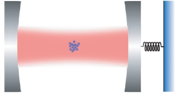
Figure 1: Schematic diagram for $N$ atoms in a single-mode optical cavity of frequency $\omega$. The cavity consists of a fixed mirror and a movable mirror, which is coupled to a mechanical oscillator.

We begin with the average of Hamiltonian Eq. (1) in boson-operator states only

$$\overset{\_}{H}\left(\alpha,\beta\right)=\langle u|H|u\rangle\text{,}$$ (3)

where the trial wave-function

$$|u\rangle=\left|\alpha\right\rangle\left|\beta\right\rangle\text{,}$$

is considered as the direct product of photon and phonon coherent states $a\left|\alpha\right\rangle=\alpha\left|\alpha\right\rangle$, $b\left|\beta\right\rangle=\beta\left|\beta\right\rangle$. In this average both photon and phonon operators are replaced by the complex boson-operator eigenvalues such that $\langle\alpha|a\left|\alpha\right\rangle=\alpha$, $\langle\alpha|a^{{\dagger}}\left|\alpha\right\rangle=\alpha^{\ast}$; $\langle\beta|b\left|\beta\right\rangle=\beta$, $\langle\beta|b^{{\dagger}}\left|\beta\right\rangle=\beta^{\ast}$. Moreover we parameterize the complex eigenvalues $\alpha$, $\beta$ as

$$\alpha=\gamma e^{i\eta}\text{,\qquad}\beta=\rho e^{i\xi}\text{.}$$

After the average in the boson coherent-state the Hamiltonian becomes

$$\overset{\_}{H}\left(\alpha,\beta\right)=(\omega-\frac{2\zeta\rho\cos\xi}{\sqrt{N}})\gamma^{2}+\omega_{b}\rho^{2}+H_{sp}\text{,}$$ (4)

in which

$$H_{sp}=\omega_{a}J_{z}+\frac{g\gamma\cos\eta\left(J_{+}+J_{-}\right)}{\sqrt{N}}$$

is an effective spin-Hamiltonian. Different from the variational method with the Holstein-Primakoff transformation, we in the following are going to diagonalize the spin Hamiltonian $H_{sp}\left(\alpha,\beta\right)$ in terms of the SCSs $|\mp\mathbf{n}\rangle$ such that

$$H_{sp}\left(\alpha,\beta\right)|\mp\mathbf{n}\rangle=E_{sp}^{\mp}|\mp\mathbf{n}\rangle\text{.}$$ (5)

We can visualize $|\mp\mathbf{n}\rangle$ as two eigenstates of a projection angular momentum operator, $\mathbf{J}\cdot\mathbf{n|\mp n}\rangle=\mp j$ $|\mp\mathbf{n}\rangle$, with $\mathbf{n}=\left(\sin\theta\cos\varphi,\sin\theta\sin\varphi,\cos\theta\right)$ being the unit vector. The directional angles $\theta$ and $\varphi$ as unknown parameters are to be determined from the eigenstate equation Eq. (5). The SCSs $|\mp\mathbf{n}\rangle$ called respectively the normal ($\Downarrow$) and inverted ($\Uparrow$) pseudospin states BMS12 can be generated from the extreme Dicke state $\left|j,-j\right\rangle$ ( $J_{z}$ $\left|j,-j\right\rangle$ $=-j\left|j,-j\right\rangle$) with the SCS transformation, $\left|\mp\mathbf{n}\right\rangle=U(\mathbf{n})\left|j,\mp j\right\rangle$. The unitary operator is given by ACG72

$$U(\mathbf{n})=e^{\frac{\theta}{2}(J_{+}e^{-i\varphi}-J_{-}e^{i\varphi})}\text{.}$$ (6)

In the SCS, spin operators satisfy the minimum uncertainty relation, for example, $\Delta J_{+}\Delta J_{-}=\left\langle J_{z}\right\rangle/2$ and therefore it is called the macroscopic quantum state. Applying the unitary transformation Eq. (6) to the eigenvalue equation Eq. (5) and using the unitary transformation relations                                                       

$$\left\{\begin{array}[]{c}U^{\dagger}J_{z}U=J_{z}\cos\theta+\frac{1}{2}e^{i\varphi}J_{-}\sin\theta+\frac{1}{2}e^{-i\varphi}J_{+}\sin\theta\text{,}\\ U^{\dagger}J_{+}U=J_{+}\cos^{2}\frac{\theta}{2}-e^{i\varphi}J_{z}\sin\theta-\frac{1}{2}J_{-}e^{2i\varphi}\sin^{2}\frac{\theta}{2}\text{,}\\ U^{\dagger}J_{-}U=J_{-}\cos^{2}\frac{\theta}{2}-e^{-i\varphi}J_{z}\sin\theta-\frac{1}{2}J_{+}e^{-2i\varphi}\sin^{2}\frac{\theta}{2}\text{,}\end{array}\right.$$

it is easy to realize that the SCSs $\left|\mp\mathbf{n}\right\rangle$ indeed are the eigenfunctions of effective spin-Hamiltonian $H_{sp}\left(\alpha,\beta\right)$ if the following conditions

$$\left\{\begin{array}[]{c}\frac{\omega_{a}}{2}e^{-i\varphi}\sin\theta+\frac{g\gamma}{\sqrt{N}}\cos\eta\left(\cos^{2}\frac{\theta}{2}-e^{-2i\varphi}\sin^{2}\frac{\theta}{2}\right)=0\text{,}\\ \frac{\omega_{a}}{2}e^{i\varphi}\sin\theta+\frac{g\gamma}{\sqrt{N}}\cos\eta\left(\cos^{2}\frac{\theta}{2}-e^{2i\varphi}\sin^{2}\frac{\theta}{2}\right)=0\text{, }\end{array}\right.$$ (7)

are satisfied. The energy eigenvalues are found as

$$E_{sp}^{\mp}=\mp\frac{N}{2}A\left(\alpha,\theta,\varphi\right)\text{,}$$

in which the parameter function is defined by

$$A\left(\alpha,\theta,\varphi\right)=\omega_{a}\cos\theta-\frac{2g}{\sqrt{N}}\gamma\cos\eta\cos\varphi\sin\theta\text{.}$$

The angle parameters $\theta$ and $\varphi$ can be determined from Eq. (7). We obtain after a tedious algebra

$$A\left(\gamma\right)=\omega_{a}\sqrt{1+f^{2}(\gamma)}\text{,}$$ (8)

which becomes a one parameter function only with

$$f(\gamma)=\frac{2g}{\omega_{a}\sqrt{N}}\gamma\text{.}$$

The total trial wave-function CNL11 ; LLM96 ; CLS04 is a direct product of the SCSs $\left|\mp\mathbf{n}\right\rangle$ and the boson coherent-states $|u\rangle$

$$\left|\psi_{\mp}\right\rangle=|u\rangle\left|\mp\mathbf{n}\right\rangle\text{.}$$ (9)

The variational energy-function in the trial state is evaluated as

$$E_{\mp}\left(\gamma,\rho,\xi\right) = \langle\psi_{\mp}|H\left|\psi_{\mp}\right\rangle$$ (10)

$$= \omega\gamma^{2}-\frac{2\zeta\rho\cos\xi}{\sqrt{N}}\gamma^{2}+\omega_{b}\rho^{2}$$

$$\mp\frac{N}{2}A\left(\gamma\right)\text{,}$$

which depends on three variational parameters $\gamma$, $\rho$, and $\xi$. The ground state can be determined by the variation of energy function $E_{\mp}\left(\gamma,\rho,\xi\right)$ with respect to the three variational parameters. The energy functions Eq. (10) are valid for any atom number $N$ unlike the variational method with the Holstein-Primakoff transformation, in which large-$N$ limit is required.

III Ground state and phase diagram

The ground state is considered as the variational minimum of energy function $E\left(\gamma,\rho,\xi\right)$ with respect to the variation parameters $\gamma$, $\rho$, $\xi$. From the usual extremum condition of the energy function $\partial E/\partial\xi=0$, and $\partial E/\partial\rho=0$ we find the relation

$$\text{ \ }\rho=\frac{\zeta\gamma^{2}}{\sqrt{N}}\text{,}$$ (11)

and the isolated parameter $\xi$ is determined as $\cos\xi=1$. Replacing the parameter $\rho$ in the energy function Eq. (10) by the relation Eq. (11) the variation-energy becomes a one-parameter function only

$$E_{\mp}(\gamma)=\omega\gamma^{2}-\frac{\zeta^{2}}{N\omega_{b}}\gamma^{4}\mp\frac{N}{2}A\left(\gamma\right)\text{.}$$ (12)

The extremum condition of energy function $\partial E_{\mp}/\partial\gamma=0$ possesses always a zero photon-number solution ($\gamma=0$), which is called the NP, if it is stable with a positive second-order derivative

$$\frac{\partial^{2}E_{\mp}(\gamma=0)}{\partial\gamma^{2}}=2\left(\omega\mp\frac{g^{2}}{\omega_{a}}\right)>0\text{.}$$ (13)

From the stability condition Eq. (13) it is easy to find that the NP state for the normal spin  ($\Downarrow$) denoted by $N_{-}$ exists only when

$$g<g_{c}=\sqrt{\omega\omega_{a}}\text{,}$$

where $g_{c}$ is the well known critical point EBr03 ; ETB03 of the phase transition between NP and SP in the Dicke model. The zero-photon solution for the inverted spin ($\Uparrow$) denoted by $N_{+}$ exists, however, in the whole region of $g$. The mechanical oscillator does not affect the NP and the critical point $g_{c}$ at all. The extremum condition of energy function for the nonzero photon solution

$$\frac{\partial E_{\mp}(\gamma)}{\partial\gamma}=0$$

becomes effectively a cubic power equation of the variable $\overset{\_}{\gamma}^{2}=\gamma^{2}/N$ seen to be

$$p_{\mp}(\overset{\_}{\gamma})=\omega-\frac{2\zeta^{2}\overset{\_}{\gamma}^{2}}{\omega_{b}}\mp\frac{g^{2}}{A(\overset{\_}{\gamma})}=0\text{,}$$ (14)

where $A(\overset{\_}{\gamma})=\omega_{a}\sqrt{1+f^{2}(\overset{\_}{\gamma})}$ with $f(\overset{\_}{\gamma})=2g\overset{\_}{\gamma}/\omega_{a}$. The Eq.(14) can be solved graphically. According to the experimental parameters BGB10 ; KMB11 , we set the atom resonant frequency $\omega_{a}=$ $1$ $MHz$ and the collective atom-field coupling strength $g$ should be in the same order BGB10 ; KMB11 to realize the Dicke phase transition. The frequency of nano-oscillator $\omega_{b}$ ranged from megahertz to gigahertz AAU09 and the photon-phonon coupling constant $\zeta$ is of the order of megahertz AKM . In the numerical evaluation the coupling constants, field frequency, and energy are measured in the unit of atom frequency $\omega_{a}$ throughout the paper. We assume $\omega_{b}=10$ in this paper. Fig. 2 displays the plots of polynomial $p_{\mp}(\overset{\_}{\gamma})$ and scaled energy

$$\varepsilon_{\mp}(\overset{\_}{\gamma})=\frac{E_{\mp}(\gamma)}{N}$$ (15)

as functions of the variable $\overset{\_}{\gamma}$ for a given photon-phonon coupling $\zeta=1$ and various atom-field coupling values to show the $g$-dependence of the solutions. The second-order derivative of the energy function

$$\frac{\mathbf{\partial}^{2}\mathbf{\varepsilon}_{\mp}\left(\overset{\_}{\gamma}\right)}{\mathbf{\partial}\overset{\_}{\gamma}^{2}}=2\left(\omega\mathbf{-}\frac{6\zeta^{2}\overset{\_}{\gamma}^{2}}{\omega_{b}}\mathbf{\mp}\frac{g^{2}\omega_{a}^{\frac{1}{2}}}{A^{\frac{3}{2}}(\overset{\_}{\gamma})}\right)$$ (16)

serves as the stability condition of the nonzero photon state. The solution of energy extremum condition Eq. (14) denoted by $\gamma_{s}^{-}$ is a stable state, which is the root of the polynomial $p_{-}(\overset{\_}{\gamma})$ with a positive slope of the curve [Fig. 2(a2)] and, therefore, the positive second-order derivative of the energy function $\partial^{2}\mathbf{\varepsilon}_{-}\left(\overset{\_}{\gamma}\right)/\partial\overset{\_}{\gamma}^{2}>0$. The state $\gamma_{s}^{-}$, which is a local minimum of the energy function [Fig. 2(b2)], is called the SP in the phase diagram. The higher value solution denoted by $\gamma_{us}^{-}$ [Fig. 2(a2)] with a negative slope (namely the negative second-order derivative of the energy function) is a unstable state corresponding to the local maximum of the energy function (b2). For the fixed photon-phonon coupling $\zeta=1$, two solutions move close to each other with the increase of the atom-field coupling $g$ and finally coincide at a critical value $g_{t}=1.763$ (a3) called the turning point, where the energy function becomes a flexing point (b3). Above this point the SP no longer exists. The unstable state $\gamma_{us}^{-}$ extends also to the NP region below the critical point $g_{c}$ seen from Fig. 2(a1), (b1). The variation of the SP-state $\gamma_{s}^{-}$ with the photon-phonon coupling $\zeta$ is shown in the Fig. 3 for a fixed atom-field coupling $g=1.5$. The two solutions $\gamma_{s}^{-}$ and $\gamma_{us}^{-}$ also move close to each other with the increase of $\zeta$. Particularly when the photon-phonon coupling reaches a critical value $\zeta=1.203$ the two states $\gamma_{s}^{-}$, $\gamma_{us}^{-}$ coincide and the energy curve becomes a flexing point corresponding to the turning point $g_{t}=1.5$ seen from Fig. 4.

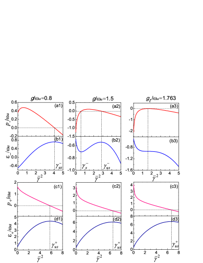
Figure 2: (Color online) Graphical solution of the energy extremum equations $p_{-}(\overset{-}{\gamma})=0$ (upper panel), $p_{+}(\overset{-}{\gamma})=0$ (lower panel) for given photon-phonon coupling $\zeta=1.0$ and different atom-field couplings $g=0.8$ (a1)(c1), $1.5$ (a2)(c2), $1.763$ (a3)(c3). The corresponding average-energy curves are plotted in (b1)(d1), (b2)(d2), (b3)(d3). $\gamma_{s}^{-}$ denotes stable nonzero photon solution of normal spin ($\Downarrow$) with a local energy minimum and $\gamma_{us}^{-}$ is the unstable one (energy maximum). There is no any stable solution for the inverted spin ($\Uparrow$) but the unstable one denoted by $\gamma_{us}^{+}$.

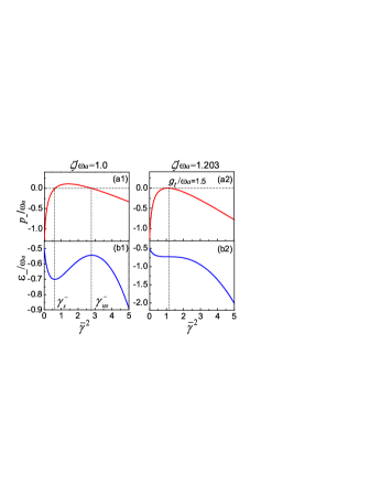
Figure 3: (Color online) $\zeta$-dependence of the nonzero photon solution of the energy extremum equation $p_{-}(\overset{\_}{\gamma})=0$ (a) and the corresponding energy curve $\varepsilon_{-}$ (b) with $\zeta=1.0$ (1), $1.203$ (2), for the fixed atom-field coupling $g=1.5$. With the increase of $\zeta$ the stable and unstable solutions move close to each other and finally coincide at the turning point seen from (a1) (a2).

For the inverted spin ($\Uparrow$) we only find the unstable nonzero photon state denoted by $\gamma_{us}^{+}$ in the system considered [Fig. 2(c)]. Fig. 4 is the phase diagram of $g$-$\zeta$ plane obtained from the extremum Eq. (14) and stability condition Eq. (16) with $\omega=1$. The mechanical oscillator does not affect the NP and the critical point $g_{c}$ between NP and SP. The SP is, however, bounded by the turning-point line $g_{t}$, beyond which the SP collapses by the resonant damping of the nano-oscillator. In the region above the turning-point line $g_{t}$ the zero photon solution $N_{+}$ of Eq. (14) still exists for the inverted spin ($\Uparrow$) and becomes the ground state. This NP with the state $N_{+}$ is denoted by the phase notation $NP(N_{+})$ in the phase diagram (Fig. 4). Thus the system undergoes an additional phase transition at the turning point $g_{t}$ from the SP to the $NP(N_{+})$.

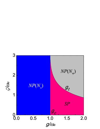
Figure 4: Phase diagram in $g$-$\zeta$ plane. The SP is restricted by two boundary lines of $g_{c}$ and $g_{t}$. When $\zeta=0$ the phase transition reduces exactly to that of Dicke model from the $NP(N_{-})$ to the SP at the critical point $g_{c}$. The region of SP extends from $g_{c}$ to infinity. On the other hand the region of SP decreases with the increase of $\zeta$ and disappears completely when $\zeta=3.0$ resulting in the direct transfer between two NP-states $N_{-}$ and $N_{+}$.

The turning point shifts back to the lower value direction of atom-field coupling $g$ with the increase of photon-phonon coupling $\zeta$ and the SP disappears completely at the value $\zeta=3$.

IV Collapse of the superradiant phase and atomic population transfer

The nano-oscillator induces collapse of the SP due to resonant damping. To see detail of the effect we study the variations of average photon number, energy and atomic population with respect to the coupling constants $g$, $\zeta$. The mean photon number in the SP is obviously

$$n_{p}=\frac{\left\langle\alpha|a^{{\dagger}}a|\alpha\right\rangle}{N}=\left(\gamma_{s}^{-}\right)^{2}\text{,}$$ (17)

here $\gamma_{s}^{-}$ means the corresponding $\overset{\_}{\gamma}$-value in the SP of normal spin ($\Downarrow$) as indicated in Figs. 2 and 3. The atomic population difference is evaluated from average of the collective pseudospin operator in the normal spin state $|-\mathbf{n\rangle}$

$$\Delta n_{a} = \frac{\left\langle-\mathbf{n}|J_{z}|-\mathbf{n}\right\rangle}{N}=\frac{\left\langle j,-j|U^{{\dagger}}(\mathbf{n})|J_{z}U(\mathbf{n})\mathbf{|}j,-j\right\rangle}{N}$$ (18)

$$= -\frac{1}{2\sqrt{1+f^{2}(\gamma_{s}^{-})}}\text{,}$$

which becomes the known value in the NP, that $\Delta n_{a}(\gamma_{-}=0)=-1/2$. While the atomic population difference in the state $N_{+}$ is $\Delta n_{a}(\gamma_{+}=0)=1/2$ indicating the atomic population inversion. The average of phonon number is proportional to the square of photon number that

$$n_{b}=\frac{\left\langle\beta|b^{{\dagger}}b|\beta\right\rangle}{N}=\frac{\zeta^{2}}{\omega_{b}^{2}}n_{p}^{2}\text{.}$$ (19)

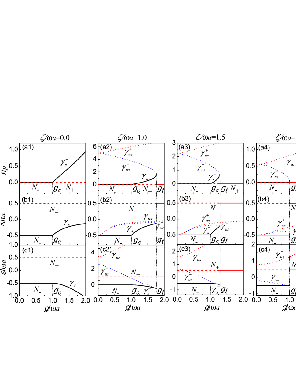
Figure 5: (Color online) The photon-phonon coupling dependence of average photon number $n_{p}$ (a), atomic population difference $n_{a}$ (b) and average energy $\varepsilon$ (c). The typical phase transition of Dicke model ($\zeta=0$) is shown in (1), where $g_{c}$ is the critical point between $NP$($N_{-}$) (black solid line) and $SP$($\gamma_{s}^{-}$) (black solid line). The SP collapses at the turning point $g_{t}$ (2), (3) and the zero photon state $N_{+}$ becomes the ground state (red solid line). The system undergoes the second phase transition from SP to the $NP(N_{+})$. When $\mathbf{\zeta=}3.0$ (4) the SP disappears and we see the direct atomic population transfer between two states $N_{-}$ and $N_{+}$ [or spin flip between normal ($\Downarrow$) and inverted ($\Uparrow$) spins]. Beyond the turning point $g_{t}$ the nonzero photon state turns back to an upper branch $\gamma_{us}^{-}$ (blue dotted line), which is unstable. $\gamma_{us}^{+}$ (red dotted line) denotes unstable state of inverted spin.

The average photon number can be considered as an order parameter with $n_{p}>0$ denoting the SP and $n_{p}=0$ for the NP. We plot in Fig. 5 the $n_{p}$ curves for different phonon-photon couplings $\zeta$ compared with the normal Dicke model ($\zeta=0$) shown in Fig. 5(1) to demonstrate the nano-oscillator induced effect. Below the critical point $g_{c}$ we have the bistable zero photon states $N_{\mp}$ , in which the $N_{-}$ (black solid line) with lower energy [Fig. 5(c)] is the ground state and $N_{+}$ is the excited state (red dash line). The phase transition from $NP(N_{-})$ to SP of the nonzero photon state $\gamma_{s}^{-}$ takes place at the critical point $g_{c}$. In this region the zero photon state $N_{+}$ (red dash lines) is still excited state with higher energy than superradiant state $\gamma_{s}^{-}$ seen from Fig. 5(c1-c3). The SP collapses at the turning point $g_{t}$ and the zero photon state $N_{+}$ of inverted spin ($\Uparrow$) (the atomic population inversion state) shown in Fig. 5(b) becomes the ground state (red solid line). An additional phase transition from SP to the $NP(N_{+})$ appears at the turning point $g_{t}$. This multiple phase transitions generated by the mechanical oscillator does not exist at all in the usual Dicke model [Fig. 5(1)]. With the increase of photon-phonon coupling $\zeta$ the region of SP is suppressed and the turning point $g_{t}$ shifts back to the lower value direction of $g$ [Fig. 5(2,3)]. The SP disappears completely at a critical value $\zeta=3$ and the phase transition becomes the transition from the $NP(N_{-})$ to $NP(N_{+})$ within the same phase of zero order-parameter $\gamma=0$ [Fig. 5(a4)] but different average energy [Fig. 5(c4)] and atomic population [Fig. 5(b4)]. We observe a interesting phenomenon of atomic population transfer (or spin flip) between two atom levels (b4). Since the atomic population inversion plays a important role in the laser physics, the controllable population transfer certainly has technical applications. Beyond the turning point $g_{t}$ the nonzero photon state turns back to a upper branch state $\gamma_{us}^{-}$ (blue dotted lines) so that we have a dual state for one value of $g$. This is similar to the optical bistability, however, the state $\gamma_{us}^{-}$ is unstable in the considered system. The unstable state $\gamma_{us}^{+}$ (red dotted lines) of inverted spin ($\Uparrow$) possesses more higher values of photon-number, atomic population, and average energy as well.

It may be worthwhile to emphasize again that the SCS variational method LLL13 has advantage to avoid the thermodynamic limit and the Dicke phase transition demonstrated in this paper is valid for arbitrary atom number $N$. We in the following section compare our results with those in the literature.

V Dicke phase transition for Rabi model

The Rabi model describes a two-level atom in a single-mode cavity Rab36 and has been widely used in atomic, optic, and condensed matter physics SZu97 . The validity of the model has been experimentally verified in various systems RBH01 ; LBM03 ; NPT01 ; FLM10 ; Lon11 ; CLO12 ; LWe11 . In the absence of the mechanical oscillator ($\zeta=0$) the Hamiltonian Eq. (1) of optomechanical cavity reduces exactly to that of the Rabi model for $N=1$. The energy function has a simple form LZL12 ; LLM96 ; CLS04 (we in this section consider only the normal spin ($\Downarrow$) and neglect the subscript ”-” for the simplicity). The energy function becomes simply

$$E\left(\gamma\right)=\omega\gamma^{2}-\frac{A(\gamma)}{2}\text{.}$$ (20)

The extremum equation $\partial E(\gamma)/\partial\gamma=0$ gives rise to the stable zero-photon solution $\gamma=0$, namely the NP, below the critical point

$$g_{c}=\sqrt{\omega\omega_{a}}.$$

The photon number in the SP above $g_{c}$ is found as

$$n_{p}=\langle\alpha|a^{{\dagger}}a|\alpha\rangle=\gamma_{s}^{2}=\frac{1}{4}\left(\frac{g^{2}}{\omega^{2}}-\frac{\omega_{a}^{2}}{g^{2}}\right),$$ (21)

which is exactly the same as the average photon number $n_{p}$ =$\langle\alpha|a^{{\dagger}}a|\alpha\rangle/N$ in the normal Dicke model ETB03 ; CLL06 ; LZL12 with $N$ atoms. The ground state energy

$$E\left(g\right)=\left\{\begin{array}[]{c}-\frac{\omega_{a}}{2}\text{, }g\leq g_{c}\text{,}\\ -\frac{\omega}{4}\left(\frac{g^{2}}{\omega^{2}}+\frac{\omega_{a}^{2}}{g^{2}}\right)\text{, }g>g_{c}\text{.}\end{array}\right.$$ (22)

equals also to the average energy of Dicke model ETB03 ; CLL06 ; LZL12 . We present the energy curves obtained from the analytic formula of Eq. (22) and the numerical diagonalization together in Fig. 6. We see the perfect coincidence in a wide range of coupling value and for both the red and blue detuning. The small deviations come out in the large detuning as shown by the dashed lines. The deviation decreases with the increase of photon-number $n$ of Fock state in the numerical diagonalization. The phase transition indeed exists in the Rabi model in agreement with the recent observation HPP15 .

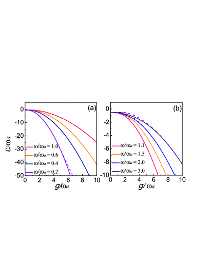
Figure 6: (Color online) The energy curves obtained from both analytic formula Eq.(22) and the numerical diagonalization with Fock state up to $300$-photon for the red detuning (a) and blue detuning (b). The deviation of numerical-diagonalization line from the analytic result is indicated by the dashed line.

VI Conclusion and discussion

The SCS variational method is a universal tool in the study of ground-states for various atom-cavity systems with arbitrary atom number $N$. The Dicke phase transition is a common phenomenon independent of the atom number $N$. The only assumption is that the cavity field is in the coherent state or in other words the macroscopic quantum state. The nano-oscillator coupled with the cavity mode by radiation-pressure does not affect the phase transition boundary from the NP to SP. However the SP state collapses at a turning point due to the resonant damping of the oscillator. As a consequence of collapse the zero-photon state-$N_{+}$ of inverted spin ($\Uparrow$) becomes a ground-state and an additional phase transition from the SP to $NP(N_{+})$ takes place at the turning point. Particularly a direct atomic population-transfer between two atom-levels is realized by the manipulation of photon-phonon coupling. This novel observation may have technical applications in laser physics. In the absence of mechanical oscillator ($\zeta=0$) our result recover the phase transition of Dicke model. The phase transition remains for Rabi model with $N=1$ in agreement with the recent observation HPP15 . This conclusion is also verified by the quantitative agreement of average energy with the result of numerical diagonalization in a wide region of coupling constant for both the red and blue detuning. The dual nonzero-photon states similar to the optical bistability are also found, however, the upper branch of state is unstable in the system considered.

VII Acknowledgments

This work was supported by the National Natural Science Foundation of China (Grant Nos. 11275118, 11404198, 91430109), and the Scientific and Technological Innovation Programs of Higher Education Institutions in Shanxi Province (STIP) (Grant No. 2014102), and the Launch of the Scientific Research of Shanxi University (Grant No. 011151801004), and the National Fundamental Fund of Personnel Training (Grant No. J1103210). The natural science foundation of Shanxi Province (Grant No. 2015011008).

References

- (1) R.H. Dicke, Phys. Rev. 93 (1954) 99.
- (2) T.C. Jarrett, C.F. Lee, and N.F. Johnson, Phys. Rev. B 74 (2006) 121301(R).
- (3) N . Lambert, C. Emary, and T. Brandes, Phys. Rev. Lett. 92 (2004) 073602.
- (4) S. Dusuel, and J. Vidal, Phys. Rev. Lett. 93 (2004) 237204.
- (5) C. Emary, and T. Brandes, Phys. Rev. Lett. 90 (2003) 044101.
- (6) C.F. Lee and N.F. Johnson, Phys. Rev. Lett. 93 (2004) 083001.
- (7) K. Hepp and E.H. Lieb, Phys. Rev. A 8 (1973) 2517.
- (8) K. Baumann, C. Guerlin, F. Brennecke, and T. Esslinger, Nature (London) 464 (2010) 1301.
- (9) K. Baumann, R. Mottl, F. Brennecke, and T. Esslinger, Phys. Rev. Lett. 107 (2011) 140402.
- (10) G. Chen, J.Q. Li, and J.-Q. Liang Phys. Rev. A 74 (2006) 054101.
- (11) C. Emary, and T. Brandes, Phys. Rev. E 67 (2003) 066203.
- (12) R. Gilmore, L.M. Narducci, Phys. Rev. A 17 (1978) 1747.
- (13) J.L. Lian,, Y.W. Zhang, and J.-Q Liang, Chin. Phys. Lett. 29 (2012) 060302.
- (14) O. Castaños, E. Nahmad-Achar, R. López-Peña, and J.G. Hirsch, Phys. Rev. A 83 (2011) 051601(R).
- (15) F. Dimer, B. Estienne, A.S. Parkins, and H.J. Carmichael, Phys. Rev. A 75 (2007) 013804.
- (16) P. Horak, and H. Ritsch, Phys. Rev. A 63 (2001) 023603.
- (17) P. Verma, A.B. Bhattacherjee, and ManMohan, Canadian Journal of Physics 90 (2012) 1223.
- (18) V.B. Braginsky, Y.I. Vorontsov, K.S. Thorne, Science 209 (1980) 547.
- (19) A. Schliesser, P. Del’Haye, N. Nooshi, K.J. Vahala, and T.J. Kippenberg, Phys. Rev. Lett. 97 (2006) 243905.
- (20) T. Corbitt, Y. Chen, E. Innerhofer, et al., Phys. Rev. Lett. 98 (2007) 150802.
- (21) S. Mancini, V.I. Man’ko, and P. Tombesi, Phys. Rev. A 55 (1997) 3042.
- (22) W. Marshall, C. Simon, R. Penrose, D. Bouwmeester, Phys. Rev. Lett. 91 (2003) 130401.
- (23) M. Aspelmeyer, T.J. Kippenberg, and F. Marquardt, arXiv:1303.0733.
- (24) N. Aggarwal, and A.B Bhattacherjee, Journal of Modern Optics 60 (2013) 1263-1272.
- (25) K. Debnath, and A.B Bhattacherjee, Commun. Theor. Phys. 64 (2015) 39.
- (26) J.L. Lian, N. Liu, J.-Q. Liang, et al, Phys. Rev. A 88 (2013) 043820.
- (27) J.P. Santos, F.L. Semião, and K. Furuya, Phys. Rev. A 82 (2010) 063801.
- (28) J.M. Radcliffe, J. Phys. A: Gen. Phys. 4 (1971) 313.
- (29) D. Markham, and V. Vedral, Phys. Rev. A 67 (2003) 042113.
- (30) A. Altland, and F. Haake, New J. Phys. 14 (2012) 073011.
- (31) X.Q. Zhao, N. Liu, and J.-Q. Liang, Phys. Rev. A 90 (2014) 023622.
- (32) M.J. Bhaseen, J. Mayoh, B.D. Simons, and J. Keeling, Phys. Rev. A 85 (2012) 013817.
- (33) M. Pinarda, Y. Hadjarb, and A. Heidmann, Eur. Phys. J. D 7 (1999) 107-116.
- (34) Y. Colombe, T. Steinmetz, G. Dubois, F. Linke, D. Hunger, and J. Reichel, Nature (London) 450 (2007) 272.
- (35) A.B. Bhattacherjee, Phys. Rev. A 80 (2009) 043607.
- (36) Y.K. Wang, and F.T. Hioe, Phys. Rev. A 7 (1973) 831.
- (37) F.T. Hioe, Phys. Rev. A 8 (1973) 1440.
- (38) T.J. Kippenberg, and K.J. Vahala, Science 321 (2008) 1172.
- (39) F. Marquardt, and S.M. Girvin, Physics 2 (2009) 40.
- (40) I. Favero, and K. Karrai, Nature Photonics 3 (2009) 201.
- (41) M. Aspelmeyer, S. Gröblacher, K. Hammerer, and N. Kiesel, J. Opt. Soc. Am. B A 27 (2010) 189.
- (42) C.A. Regal and K.W. Lehnert, J. Phys: Conf. Ser. 264 (2011) 012025.
- (43) S. Gröblacher, K. Hammerer, M.R. Vanner, and M. Aspelmeyer, Nature (London) 460 (2009) 724.
- (44) J.P. Santos, F.L. Semião, and K. Furuya, Phys. Rev. A 82 (2010) 063801.
- (45) Y. Chang, H. Ian, and C.P. Sun, J. Phys. B: At. Mol. Opt. Phys. 42 (2009) 215502.
- (46) F.T. Arecchi, and E. Courtens, and R. Gilmore, and H. Thomas, Phys. Rev. A 6 (1972) 2211.
- (47) Y.-Z. Lai, J.-Q. Liang, H.J. W. Müller-Kirsten, and J.-G. Zhou, Phys. Rev. A 53 (1996) 3691.
- (48) Z.-D. Chen, J.-Q. Liang, S.-Q. Shen, and W.-F. Xie, Phys. Rev. A 69 (2004) 023611.
- (49) G. Anetsberger, O. Arcizet, Q.P. Unterreithmeier, et.al, Nat. Phys. 5 (2009) 909.
- (50) I.I. Rabi Phys. Rev. 49 (1936) 324.
- (51) M.O. Scully, and M.S. Zubairy, Quantum optics (Cambridge University Press, Cambridge) (1997).
- (52) J.M. Raimond, M. Brune, and S. Haroche, Rev. Mod. Phys. 73 (2001) 565.
- (53) D. Leibfried, R. Blatt, C. Monroe, and D. Wineland, Rev. Mod. Phys. 75 (2003) 281.
- (54) Y. Nakamura, Y.A. Pashkin, and J.S. Tsai, Phys. Rev. Lett. 87 (2001) 246601.
- (55) P. Forn-Díaz, J. Lisenfeld, D. Marcos, et al., Phys. Rev. Lett. 105 (2010) 237001.
- (56) S. Longhi, Opt. Lett. 36 (2011) 3407.
- (57) A. Crespi, S. Longhi, and R. Osellame, Phys. Rev. Lett. 108 (2012) 163601.
- (58) J.-Q. Liang, and L.F. Wei, Advances In Quantum Physics 18-48 (Beijing) 2011.
- (59) M-J. Hwang, R. Puebla, and M.B. Plenio, Phys. Rev. Lett. 115 (2015) 180404.