Self-synchronization and Self-stabilization of 3D Bipedal Walking Gaits

Abstract

This paper seeks insight into stabilization mechanisms for periodic walking gaits in 3D bipedal robots. Based on this insight, a control strategy based on virtual constraints, which imposes coordination between joints rather than a temporal evolution, will be proposed for achieving asymptotic convergence toward a periodic motion. For planar bipeds with one degree of underactuation, it is known that a vertical displacement of the center of mass—with downward velocity at the step transition—induces stability of a walking gait. This paper concerns the qualitative extension of this type of property to 3D walking with two degrees of underactuation. It is shown that a condition on the position of the center of mass in the horizontal plane at the transition between steps induces synchronization between the motions in the sagittal and frontal planes. A combination of the conditions for self-synchronization and vertical oscillations leads to stable gaits. The algorithm for self-stabilization of 3D walking gaits is first developed for a simplified model of a walking robot (an inverted pendulum with variable length legs), and then it is extended to a complex model of the humanoid robot Romeo using the notion of Hybrid Zero Dynamics. Simulations of the model of the robot illustrate the efficacy of the method and its robustness.

I Introduction

Despite a growing list of bipedal robots that are able to walk in a laboratory environment or even outdoors, stability mechanisms for 3D bipedal locomotion remain poorly understood. It would be very satisfying to be able to point at a robot and say, “it can execute an asymptotically stable walking gait, and the stability is achieved through such and such theorem, principle, method, etc.” For planar (aka 2D) robots with one degree of underactuation, virtual constraints and hybrid zero dynamics provide an integrated gait and controller design method that comes with a formal closed-form stability guarantee [32][pp. 128-135]. Moreover, the stability condition is physically meaningful: the velocity of the center of mass (CoM) at the end of the single support phase must be directed downward [6].

For fully actuated 3D bipeds and for 3D bipeds with a special form of underactuation, the 2D results extend nicely [33, 30]. But for 3D robots with more than one degree of underactuation, not much is known.

Basing the control law design of a fully actuated robot on a model with either a passive ankle or a point foot contact is an interesting intermediate view of the robot. Even in case of a fully actuated robot, the ankle torques in the frontal and sagittal planes are limited by the size of the foot. A model with two degrees of underactuation is therefore useful in order to avoid the use of these torques for a nominal (unperturbed) gait. This allows the limited ankle torque to be saved for adapting the foot orientation in case of uneven terrain or for increasing the robustness of the control strategy in the face of perturbations.

The possibility and interest of extending the method of virtual constraints to robot models with two degrees of underactuation have been shown in [7, 26, 17, 1, 12]. While the implementation of the control strategy is quite straightforward, the choice of the virtual constraints is not obvious. Their selection is often based on an optimization process and choice of appropriate controlled outputs and/or the introduction of a high-level event-based control strategy, neither of which provides insight into the stability mechanism. The objective of this paper is to provide some qualitative results on gait characteristics that when used to define virtual constraints lead to asymptotically stable walking.

In contrast to fully actuated bipedal walking, passive walking [20, 21] can be seen as an emergent behavior, where alternating leg impacts of a biped and the pull of gravity combine to produce asymptotically stable motions on mild downward slopes. The obtained gait is very efficient from an energy consumption point of view and can be extended to walking on flat ground [29, 8, 14]. One shortcoming of such an approach is limited robustness with respect to perturbations.

As there is no actuation in passive robots, the obtained walking gaits may be called self-stable. The self-stability property is well understood in 2D walking gaits [5, 24], however, little is known on why a passive robot can demonstrate stable walking in 3D. Only a few studies have been devoted to the investigation of analytical properties that lead to asymptotically stable gaits in 3D underactuated robots [16, 26]. In [7] for example, it has been shown that when a controller design method that yielded asymptotically stable gaits in planar underactuated walking [5] is applied to 3D walking, unstable solutions are common.

The notion of self-synchronization, introduced in [25] and generalized in [26], sheds some light on the stability mechanisms in 3D legged locomotion.

The aim of the paper is to provide insight towards understanding the mechanisms of asymptotic stability in periodic walking of 3D underactuated robots. Using a control law based on virtual constraints for 3D bipedal robots with two degrees of underactuation, our objective is to propose virtual constraints leading to self stabilization. In other words, without the use of event-based control, the obtained gaits are asymptotically stable.

As opposed to the formal theorems proven in [32] for 2D robots, and for the self-synchronization of the 3D LIP [25, 26] the results here for 3D will be numerical in nature. By normalizing the studied model, qualitative gait features leading to asymptotically stable periodic orbits will be uncovered, nevertheless. The method will be first demonstrated on an inverted pendulum model and then will be extended to a full model of the humanoid Romeo [27, Chapter 7], shown in Figure 1.

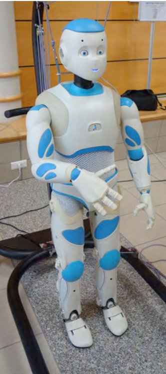
Figure 1: The humanoid robot Romeo developed by Aldebaran robotics.

The remainder of the paper is organized as follows. In Section II, as background, the control method based on virtual constraints for a 3D humanoid robot with 2 degrees of underactuation is recalled. The stability of the full-order model of the robot is discussed in relation to an induced reduced-order model, called the Hybrid Zero Dynamics (HZD). In Section III, the difficulty of choosing appropriate virtual constraints is highlighted. Moreover, an important difference between planar and 3D walking, which is due to an increase of the degrees of underactuation, is illustrated. In particular, it is shown that unlike the planar case, where at the impact the set describing the final configuration of the robot in the reduced model consists of a single point, in 3D walking with two degrees of underactuation, this set is a manifold of dimension one. In Section IV, where we study a very simplified model of a humanoid robot, the role of this subset in achieving self-synchronization for the Linear Inverted Pendulum model (LIP) will be demonstrated. Moreover, a new geometric interpretation of the self-synchronization property will be provided in this section. Subsequently, in Section IV-D, we introduce vertical oscillations of the CoM for the pendulum model. Self-stabilization properties will be numerically studied in Section IV-E. In Section V, the results obtained on the simplified model will be extended to a realistic model of a humanoid robot. A numerical study shows how the stability properties obtained for the pendulum extend to a complete model of a bipedal robot. Simulation results illustrate the efficiency of the approach.

II Background: A Reduced-order Model Associated with Underactuation

This section reviews how to create a reduced-order model within the full-dimensional hybrid model of a bipedal robot with the following properties:

• the dimension of the reduced-order model is determined by the number of degrees of underactuation of the robot;

• the periodic orbits of the reduced-order model are periodic orbits of the robot;

• locally exponentially stable periodic orbits in the reduced-order model can always be rendered locally exponentially stable in the full-order model of the robot through the use of feedback control; and

• no approximations are being made.

Based on the above properties, it can be seen that the reduced-order model captures the effects of underactuation on the design of stabilizing feedback control laws for bipedal robots. Later sections of the paper develop properties of this reduced-order model that lead to existence of locally exponentially stable walking gaits.

II-A Full-order hybrid model

Let $q\in{\cal Q}$ denote the generalized coordinates for a humanoid robot in single support (one foot on the ground) and assume the stance ankle has two DoFs (pitch and roll), both assumed to be passive, that is, unactuated. Typically, $q$ consists of body coordinates, such as joint angles of the stance leg, swing leg, upper-body, and in our case, two additional world-frame coordinates capturing the pitch and roll degrees of freedom in the ankle. The robot is assumed to have right/left symmetry and the gait studied corresponds to walking along a straight line in the sagittal plane. Moreover, the gait is assumed to be composed of single support phases separated by impacts, which are modeled as instantaneous changes of support. At each transition, a relabeling of the joint variables is introduced. This relabeling allows us to work with a single model of the robot.

The Lagrangian is assumed to have the form

$$L(q,\dot{q})=\frac{1}{2}\dot{q}^{T}D(q)\dot{q}-V(q),$$

and the single support model is given by the standard Lagrange equations

$$\frac{\text{d}}{\text{d}t}\frac{\partial L(q,{\dot{q}})}{\partial\dot{q}}-\frac{\partial L(q,{\dot{q}})}{\partial q}=Bu,$$ (1)

where the $N\times(N-2)$ torque distribution matrix $B$ is constant and has rank $N-2$, and $u$ is an $(N-2)$-dimensional vector associated to the torques of the joint coordinates.

Equation (1) can also be written in the form

$$D(q)\ddot{q}+H(q,\dot{q})=Bu,$$ (2)

where $D(q)$ is the (positive definite) inertia matrix, and $H(q,\dot{q})$ groups the centrifugal, Coriolis and gravity terms. Letting $x=[q^{\top},\dot{q}^{\top}]^{\top}$, standard calculations lead to a state-variable model

$$\dot{x}=f(x)+g(x)u,$$ (3)

which is affine in the control torques.

For simplicity, impacts are assumed to occur with the swing foot parallel to the walking surface. Let

$$\mathcal{S}:=\{x~{}|~{}z_{s}=0,\;\dot{z}_{s}<0\},$$ (4)

where $z_{s}$ is the height of the swing foot above the walking surface. It is assumed that $\mathcal{S}$ is a smooth $(2N-1)$-dimensional manifold in the state space of the robot. The widely used impact model of Hurmuzlu [15] leads to an algebraic representation of the jumps in the velocity coordinates when the swing foot contacts the ground, and hence to a hybrid model of the robot:

$$\begin{array}[]{llll}\dot{x}&=f(x)+g(x)u,&x^{-}&\notin\mathcal{S},\\ x^{+}&=\varDelta(x^{-}),&x^{-}&\in\mathcal{S},\end{array}$$ (5)

where $x^{+}:=\lim_{\tau\searrow t}x(\tau)$ (resp. $x^{-}:=\lim_{\tau\nearrow t}x(\tau)$) is the state value just after (resp. just before) impact. The control-affine ordinary differential equation (ODE) describes the dynamics of the swing phase, whereas the algebraic equation describes the impacts of the swing foot with the ground. This algebraic equation can be decomposed into as follows:

$$\begin{array}[]{ll}q^{+}&=\varDelta_{q}(q),\\ \dot{q}^{+}&=\varDelta_{\dot{q}}(q)\dot{q}^{-}.\end{array}$$ (6)

The first matrix equation of (6) describes the relabelling of the coordinates at impact, while the second define the jump velocity coordinates.

II-B Virtual constraints and an exact reduced-order model

It is well understood in mechanics that a set of (regular) holonomic constraints applied to a Lagrangian model of a mechanical system leads to another Lagrangian model that has dimension equal to the dimension of the original model minus twice the number of independent constraints. In the case of mechanical systems, the constraints are imposed by a vector of generalized forces (aka Lagrange multipliers) that can be computed through the principle of virtual work. When computing the resulting reduced-order model, no approximations are involved, and solutions of the reduced-order model are solutions of the original model along with the inputs arising from the Lagrange multipliers.

Virtual holonomic constraints are functional relations on the configuration variables of a robot’s model that are achieved through the action of the robot’s joint torques and feedback control instead of physical contact forces. They are called virtual because they can be re-programmed on the fly in the control software. Like physical constraints, under certain regularity conditions, virtual constraints induce a low-dimensional invariant model called the zero dynamics [3, 31, 32]. A detailed comparison of “physical constraints” versus “virtual constraints” is provided in [13]. In the following, a brief overview is given.

A total of $N-2$ virtual constraints can be generated by the $N-2$ actuators. The virtual constraints are first expressed as outputs applied to the model (3), and then a feedback controller is designed that asymptotically drives them to zero. One such controller, based on the computed torque, is given in the Appendix; others can be found in [2]. Here, the virtual constraints will be expressed in the form

$$y=h({q}):=q_{\rm c}-h_{d}(q_{\rm f}),$$ (7)

where $q_{\rm c}\in{\cal Q}_{\rm c}\subset\mathbb{R}^{(N-2)}$, and $q_{\rm f}\in{\cal Q}_{\rm f}\subset\mathbb{R}^{2}$ with $(q_{\rm c},q_{\rm f})$ forming a set of generalized configuration variables for the robot, that is, such that a diffeomorphism

$$F:{\cal Q}_{\rm c}\times{\cal Q}_{\rm f}\to{\cal Q}$$

exists. The variables $q_{\rm c}$ represent physical quantities that one wishes to “control” or “regulate”, while the variables $q_{\rm f}$ remain “free”. Later, a special case of $h_{d}(q_{\rm f})$ will be employed based on a gait phasing variable, which makes it easier to interpret the virtual constraints in many instances.

When the virtual constraints are satisfied, the relation $q_{\rm c}=h_{d}(q_{\rm f})$ leads to the mapping $F_{c}:{\cal Q}_{\rm f}\to{\cal Q}$ by

$$F_{c}(q_{\rm f}):=F(h_{d}(q_{\rm f}),q_{\rm f})$$ (8)

being an embedding; moreover, its image defines a constraint manifold in the configuration space, namely

$$\tilde{{\cal Q}}=\left\{q\in{\cal Q}~{}|~{}q=F_{c}(q_{\rm f}),~{}q_{\rm f}\in Q_{\rm f}\right\}.$$ (9)

The constraint surface for the virtual constraints is

$$\mathcal{Z}: =\{(q,\dot{q})\in T{\cal Q}~{}|y=h(q)=0,~{}\dot{y}=\frac{\partial h(q)}{\partial q}\dot{q}=0\}$$

$$=\{(q,\dot{q})\in T{\cal Q}~{}|q=F_{c}(q_{\rm f}),\dot{q}=J_{c}(q_{\rm f})\dot{q}_{\rm f},~{}~{}(q_{\rm f},\dot{q}_{\rm f})\in T{\cal Q}_{\rm f}\},$$ (10)

where

$$J_{c}(q_{\rm f}):=\frac{\partial F_{c}(q_{\rm f})}{\partial q_{\rm f}}.$$ (11)

The terminology “zero dynamics manifold” comes from [3]. It is the state space for the internal dynamics compatible with the outputs being identically zero. For the underactuated systems studied here, the dimension of the zero dynamics manifold is $4$, due to the assumption of two degrees of underactuation.

Let $B^{\perp}$ be the left annihilator of $B$, that is, a $2\times N$ matrix of rank $2$ such that $B^{\perp}B=0$. Lagrange’s equation (1) then gives

$$\frac{\text{d}}{\text{d}t}\big{(}B^{\perp}\frac{\partial L}{\partial\dot{q}}\big{)}=B^{\perp}\frac{\partial L}{\partial q},$$

because $B^{\perp}Bu=0$. The term $B^{\perp}\frac{\partial L}{\partial\dot{q}}$ is a form of generalized angular momentum.

Restricting the full-system to the the zero dynamics manifold, gives

$$\dot{\sigma}_{\rm f}=\kappa(q_{\rm f},\dot{q}_{\rm f}),$$

where

$$\sigma_{\rm f} :=M(q_{\rm f})\dot{q}_{\rm f}$$

$$\kappa(q_{\rm f},\dot{q}_{\rm f}) :=\left.B^{\perp}\frac{\partial L(q,\dot{q})}{\partial q}\right|_{\begin{array}[]{l}q=F_{c}(q_{\rm f})\\ \dot{q}=J_{c}(q_{\rm f})\dot{q_{\rm f}}\end{array}}.$$ (14)

The invertibility of $M(q_{\rm f})$ is established in [13] under the assumption that the decoupling matrix used in (71) is full rank.

$$z=\left[\begin{array}[]{c}z_{1}\\ z_{2}\end{array}\right]:=\left[\begin{array}[]{c}q_{\rm f}\\ \sigma_{\rm f}\end{array}\right]$$

gives

$$\dot{z} =\left[\begin{array}[]{c}M^{-1}(z_{1})z_{2}\\ \bar{\kappa}(z_{1},z_{2})\end{array}\right]$$ (17)

$$=:f_{zero}(z),$$

where $\bar{\kappa}(z_{1},z_{2})=\kappa(z_{1},M^{-1}(z_{1})z_{2})$. The properties of this four-dimensional system are determined by the Lagrangain dynamics of the full-order model and the choice of the virtual constraints through the mapping (8). The form of the model is similar to the one used to analyze planar systems with one degree of underactuation [32, Remark 5.2].

II-C Reduced-order hybrid model (hybrid zero dynamics)

Analogous to the full-order hybrid model (5) is the so-called hybrid zero dynamics in which the zero dynamics manifold must satisfy

$$\varDelta(\mathcal{S}\cap\mathcal{Z})\subset\mathcal{Z}.$$ (18)

This condition means that when a solution evolving on $\mathcal{Z}$ meets the switching surface, $\mathcal{S}$, the new initial condition arising from the impact map is once again on $\mathcal{Z}$.

The invariance condition (18) is equivalent to

$$0= h\circ\varDelta_{q}(q)$$ (19)

$$0= \left.\frac{\partial h(\bar{q})}{\partial q}\right|_{\bar{q}=\varDelta_{q}(q)}\varDelta_{\dot{q}}(q)\,\dot{q}$$ (20)

for all $(q;\dot{q})$ satisfying

$$h(q)=0,~{}~{}\frac{\partial h(q)}{\partial q}\dot{q}= 0$$ (21)

$$z_{s}(q)=0,~{}~{}\dot{z}_{s}(q,\dot{q})< 0.$$ (22)

At first glance, these conditions may appear to be difficult to meet. In the case of models with one degree of underactuation, however, it is known that if a single non-trivial solution of the zero dynamics satisfies these conditions, then all solutions of the zero dynamics will satisfy them [32, Thm. 5.2]. In the case of systems with more than one degree of underactuation, systematic methods have been developed which modify the virtual constraints “at the boundary” and allow the conditions to be met [22]. Very straightforward implementations of the result are presented in a robotics context in [4] and [11], and we refer the reader to these paper for the details.

With the invariance condition of the impact map, the reduced order hybrid system, called hybrid zero dynamics(HZD), can be written in the form

$$\Sigma_{\rm zero}:\begin{cases}\begin{aligned} \dot{z}&=f_{\rm zero}(z),&z^{-}&\notin\mathcal{S}\cap\mathcal{Z}\\ z^{+}&=\varDelta_{{\rm zero}}(z^{-}),&z^{-}&\in\mathcal{S}\cap\mathcal{Z},\end{aligned}\end{cases}$$ (23)

with $\varDelta_{{\rm zero}}:=\left.\varDelta\right|_{\mathcal{S}\cap\mathcal{Z}}$. It is proven in [32] that solutions of (23) lift to solutions of (5); indeed, (8) results in

$$q(t) =F_{c}(z_{1}(t))$$

$$\dot{q}(t) =J_{c}(z_{1}(t))\dot{z}_{1}(t)$$

$$=J_{c}(z_{1}(t))M^{-1}(z_{1}(t))z_{2}(t).$$

It is also proven in [32] that locally exponentially stable periodic solutions of (23) lift to solutions of (5), which can be locally exponentially stabilized.

Remark 1: Low-dimensional pendulum models are approximate representation of the the swing phase dynamics of a robot, and normally when they are used, the impact map is ignored. The zero dynamics is an exact low-dimensional model that captures the underactuated nature of the robot, and moreover, the hybrid zero dynamics is an exact low-dimensional “subsystem” of the full-order hybrid model that captures the underactuated dynamics of the hybrid model.

III Self-stability and the HZD

The use of the virtual constraints allows the stability of the full-order model to be studied on the HZD. For a system of two degrees of underactuation, the HZD is reduced to a system of dimension four for any number of actuated joints. The associated Poincaré map has dimension three. This paper seeks conditions for the eigenvalues of the Jacobian of the Poincaré map to lie within the unit circle, thereby assuring local exponential stability of a periodic orbit. More precisely, this paper seeks guidelines for the selection of the virtual constraints so that eigenvalues of the Jacobian lie within the unit circle.

Once the virtual constraints are defined, we know how to write a control law that drives them to zero and the walking gait will be stable or not depending on the stability of the HZD. If the chosen virtual constraints induce stable walking, we will call this self-stability, in analogy with passive walkers.

III-A Choosing the virtual constraints by physical intuition

Choosing the virtual constraints (7) means not only selecting $h_{d}(q_{\rm f})$, but also $q_{\rm f}$ and $q_{\rm c}$. One objective of this work is to give a physical interpretation of stability of walking; thus, we choose a set of variables $q_{\rm c}$, $q_{\rm f}$ that are physically meaningful. Several choices seem possible. Since the effect of gravity appears to be crucial and the stance ankle is supposed to be unactuated in the sagittal and frontal planes, the free variables are chosen as the position of the CoM in the horizontal plane $x_{M},~{}y_{M}$. Moreover, to make our results independent of the step width $D$ and length $S$, we consider normalized variables, namely, $q_{\rm f}=(X,Y)^{\top}$, $X=\frac{x_{M}}{S}$ and $Y=\frac{y_{M}}{D}$.

Concerning the controlled variables, in principle, we wish to use meaningful coordinates that appear in both models that we will study in the next sections, that is, a simplified inverted pendulum model and a realistic model of Romeo. Since the horizontal position of the CoM is used in $q_{\rm f}$, it makes sense to consider the vertical position $z_{M}$ as one of the coordinates. Moreover, we also include the Cartesian position of the swing foot tip as a part of the controlled variables because these variables have a significant contribution to the change of support. Hence, for the simplified model of Section IV, the set of controlled variables will be $q_{\rm c}=(z_{M},X_{s},Y_{s},z_{s})$ where $z_{s}$ is the vertical position of the swing foot and $X_{s},Y_{s}$ are normalized horizontal positions of the swing foot. For the complete model of Romeo and other realistic bipeds, $q_{\rm c}$ will consist of the variables just listed for the simplified model, together with a minimal set of body coordinates to account for the remaining actuators on the robot. For Romeo, this will mean adding the orientation of the swing foot, and remaining joints in the torso and stance leg as described in Section V.

III-B From one degree of underactuation to two degrees of underactuation

By definition, the condition of transition from one step to the next is defined by (4). In this condition, the vertical velocity of the foot being negative at impact ensures a well-defined transversal intersection of the solution with the transition set. In the following discussion, we compare the set of possible configurations of the robot at the change of support in the case of one degree of underactuation versus two degrees of underactuation.

In the context of the virtual constraints, the evolution of the swing leg is imposed as a function of $q_{\rm f}$. Thus, the switching condition can be viewed as a condition on the free configuration $q_{\rm f}$. We will define a switching configuration manifold $\mathbb{S}$:

$$\mathbb{S}=\left\{q_{\rm f}|z_{s}^{d}(q_{\rm f})=0\right\}.$$ (24)

where $z_{s}^{d}$ is the virtual constraint for the height of the swing leg.

In the case of one degree of underactuation, the switching configuration manifold contains two points corresponding to the final value $q_{\rm f}^{-}$ of the periodic motion and the initial one $q_{\rm f}^{+}$, and a proper impact only requires $\dot{z}<0$ at the end of the step. For planar walking in the sagittal plane [32], the stability condition is determined completely by the periodic motion itself, in other words, it is independent of the choice of virtual constraints that induce it. Moreover, the stability condition is physically meaningful: the velocity of the CoM at the end of the single support phase (for the periodic motion) must be directed downward [6].

In the case of two degrees of underactuation, the manifold (24) depends on at least two free variables $X$ and $Y$, and therefore under mild regularity conditions it includes an infinite number of points. Hence, the switching configuration manifold of the robot right before the impact is represented by the solutions of

$$z_{s}^{d}(q_{\rm f})=z_{s}^{d}(X,Y)=0.$$ (25)

Moreover, for two degrees of underactuation, it has been shown that a given periodic gait can be asymptotically stable or unstable depending on the choice of the virtual constraints used to induce the motion [7]. We want to understand how this happens.

As a first observation, the choice of the virtual constraint, $z_{s}^{d}$, clearly affects the set of free variables belonging to the switching manifold:

$$\mathbb{S}=\left\{(X,Y)|z_{s}^{d}(X,Y)=0\right\}.$$ (26)

We will show in this paper that the shape of the switching manifold (26) has a crucial effect on the stability of walking. In particular, we show that

• in the case of the Linear Inverted Pendulum (LIP), a very common simplified model for a humanoid robot, a condition to obtain self-synchronization between the model’s motions in the lateral and sagittal planes is obtained as a condition on the tangent of $\mathbb{S}$ at the point where it is intersected by the periodic orbit; and

• when the LIP model is extended to an inverted pendulum model with a stance leg of variable length, self-synchronization plus a downward motion of the CoM yields self-stability of a periodic motion.

The results are then extended to a realistic model of the humanoid Romeo and illustrated in simulation.

IV Simple model: Variable Length Inverted Pendulum

Two of the main features involved in dynamic walking are the role of gravity and the limited torque available at the stance ankle before the foot rolls about one of its edges. Emphasizing these aspects, the inverted pendulum model has been used in numerous humanoid walking control applications, such as [18], [9], and [19].

IV-A Modeling of a Variable Length Inverted Pendulum

In recognition of this, the proposed methodology is first presented on a two-legged inverted pendulum, which consists of two telescoping massless legs and a concentrated mass at their intersection, called the hips; see Figure 2. The stance leg is free to rotate about axes $\mathbf{s}_{0}$ and $\mathbf{n}_{0}$ at the ground contact and the length of each leg can be modified through actuation, allowing a desired vertical motion of the pendulum to be obtained. We also assume that the actuation of the swing leg will allow a controlled displacement of the swing leg end via hip actuators and control of the leg length.

Figure 2: A simplified model of 3D biped robot. Each leg is massless and has variable length. At the contact point, the stance leg rotates passively around axes $\mathbf{s}_{0}$ and $\mathbf{n}_{0}$, the rotation around axis $\mathbf{a}_{0}$ is not considered since this rotation is inhibited by friction in normal biped locomotion. The swing leg has a fully actuated spherical joint with respect to the concentrated mass of the hip.

The configuration of the robot is defined via the position of the concentrated mass $(x_{M},y_{M},z_{M})$ with respect to a reference frame attached to the stance foot and the position of the swing leg tip, denoted by $(x_{s},y_{s},z_{s})$. Angular momenta along axes $\mathbf{s}_{0}$ and $\mathbf{n}_{0}$ are denoted by $\sigma_{x}$ and $\sigma_{y}$. In order to explore simultaneously the existence and stability of periodic orbits as a function of step length and width, a dimensionless dynamic model of the pendulum will be used [6]. The normalizing scaling factors applied along axes $\mathbf{s}_{0}$ and $\mathbf{n}_{0}$ depend on desired step length $S$, desired step width $D$, and the mass $m$ of the robot. Thus, a new set of variables is defined: $(X,Y,z_{M},X_{s},Y_{s},z_{s},\sigma_{X},\sigma_{Y})=(\frac{x}{S},\frac{y}{D},z_{M},\frac{x_{s}}{S},\frac{y_{s}}{D},z_{s},\frac{\sigma_{x}}{mD},\frac{\sigma_{y}}{mS})$.

The variables $(z_{M},X_{s},Y_{s},z_{s})$ will be the controlled variables $q_{\rm c}$, whose evolution will be determined by virtual constraints as a function of $q_{\rm f}=(X,Y)$.

The height of the CoM and its vertical velocity are then expressed as functions of its horizontal position and velocity:

$$z_{M}^{d} =f(X,Y)$$ (27)

$$\dot{z}_{M}^{d} =\frac{\partial f(X,Y)}{\partial X}\dot{X}+\frac{\partial f(X,Y)}{\partial Y}\dot{Y}$$

Since the legs are massless, the position of the swing leg tip and its time derivative do not affect the dynamic model and thus have no effect on the evolution of the biped during single support. The moment balance equation of the pendulum around the rotation axis $\mathbf{s}_{0}$ and $\mathbf{n}_{0}$ directly yields the equation of the zero dynamics,

$$\left\{\begin{aligned} \dot{\sigma}_{x}&=-mgy_{M},\\ \dot{\sigma}_{y}&=mgx_{M}.\end{aligned}\right.$$ (28)

For this simple model, the angular momentum is simply

$$\left\{\begin{aligned} \sigma_{x}&=m\dot{z}_{M}y_{M}-mz_{M}\dot{y}_{M},\\ \sigma_{y}&=-m\dot{z}_{M}x_{M}+mz_{M}\dot{x}_{M},\end{aligned}\right.$$ (29)

Using the normalized coordinates, the zero dynamics model (17) with $z_{2}=\sigma_{f}=[\sigma_{X},\sigma_{Y}]^{\top}$ can be written as

$$\left\{\begin{aligned} \dot{q}_{\rm f}&=M_{XY}^{-1}\sigma_{f},\\ \dot{\sigma}_{X}&=-gY,\\ \dot{\sigma}_{Y}&=gX,\end{aligned}\right.$$ (30)

where

$$M_{XY}=\begin{bmatrix}\frac{\partial f(X,Y)}{\partial X}Y&\frac{\partial f(X,Y)}{\partial Y}Y-f(X,Y)\\ -\frac{\partial f(X,Y)}{\partial X}X+f(X,Y)&-\frac{\partial f(X,Y)}{\partial Y}X\end{bmatrix}.$$

We assume that once the tip of the swing leg hits the ground, that is, when $z\in\mathcal{S}\cap\mathcal{Z}$, the legs immediately swap their roles; thus, we assume that the double support phase is instantaneous.

The state right before (after) the swapping of roles of the legs is denoted by the exponent ^- (⁺). During the swapping of the support leg, the configuration of the robot is fixed, but the reference frame is changed since it is attached to the new stance leg tip. From the geometry, for normalized variables we have:

$$\left\{\begin{aligned} X^{+}&=X^{-}-X_{s}^{-},\\ Y^{+}&=-Y^{-}+Y_{s}^{-},\end{aligned}\right.$$ (31)

where the change of sign in the second equation corresponds to the change of direction of the axis $\mathbf{n}_{0}$. Since the velocity of the CoM of a biped with massless legs is conserved in the transition, we also have

$$\left\{\begin{aligned} \dot{X}^{+}&=\dot{X}^{-},\\ \dot{Y}^{+}&=-\dot{Y}^{-}.\end{aligned}\right.$$ (32)

The design of the switching manifold $\mathbb{S}$ defined via $z_{s}^{d}(X,Y)$, and the transition condition (31) affected by $X^{-}$, $Y^{-}$ defined via $X_{s}^{d}(X,Y)$ and $Y_{s}^{d}(X,Y)$, are discussed in the next section.

IV-B Virtual constraints for the swing leg

Assume that a desired periodic motion is characterized by an initial free configuration for the single support phase $X_{0},Y_{0}$ and a final free configuration $X_{f},Y_{f}$. Due to the normalization of the variables with respect to the gait length and width, and the desired symmetry between left and right support, we have $X_{f}-X_{0}=1$ and $Y_{0}+Y_{f}=1$. Our initial objective is to define a virtual constraint for the height of the swing foot, $z_{s}^{d}$, as a function of $X$ and $Y$. This virtual constraint takes the value $0$ for $X=X_{0},Y=Y_{0}$ and $X=X_{f},Y=Y_{f}$, and is positive in between during the single support phase.

Inspired by [25], we propose

$$z_{s}^{d}=Z_{se}(X,Y)=\nu_{z}S_{a}(X,Y),$$ (33)

where $\nu_{z}$ is a negative parameter that adjusts the height of the swing foot during a step and $S_{a}(X,Y)$ is

$$S_{a}(X,Y)=(X-X_{a})^{2}+CY^{2}-((X_{0}-X_{a})^{2}+CY_{0}^{2})$$ (34)

with

$$X_{a}=\frac{(X_{f}+X_{0})+C(Y_{f}-Y_{0})}{2}.$$ (35)

With this choice the ellipse-shaped switching manifold is defined by

$$\mathbb{S}=\left\{(X,Y)|S_{a}(X,Y)=0\right\},$$ (36)

and is illustrated in Figure 3.

(a) The mass motion starts on the switching manifold on one stance leg

(b) When the mass crosses the switching manifold, the support leg is changed

Figure 3: The switching manifold (red ellipse) defines the position of the CoM where the swing leg hits the ground, with an instantaneous change of support leg.

Remark 2: The shape of the switching manifold is somewhat arbitrary. We will see in the stability analysis done in the following section that only the tangent of the switching manifold at $X_{f},Y_{f}$ will be used. The orientation of this tangent is characterized by the parameter $C$, and its effect will be studied in detail.
The virtual constraint imposed for the height of the swing foot defines the switching manifold and is crucial for the stability of a gait. The virtual constraint associated with the horizontal position of the swing foot will allow us to impose where the swing foot is placed on the ground.

In the case studied, the horizontal position of the swing foot is controlled to obtain an ($X_{0},Y_{0})$-invariant gait; that is, the starting position of the CoM with respect to the stance foot will be $(X_{0},Y_{0})$ independent of any error in the previous step. Based on (31), the horizontal motion of the swing leg must be such that when $S_{a}(X,Y)=0$ (i.e., when the leg touches the ground), the desired position $X_{s}^{-}=-X_{0}+X$, $Y_{s}^{-}=Y_{0}+Y$ is reached.

To achieve this objective, at the end of the motion of the swing foot, the virtual constraints are defined by:

$$X_{s}^{d}=X_{se}(X,Y)=\left(1-\nu_{X}S_{a}(X,Y)\right)\left(-X_{0}+X\right),$$ (37)

$$Y_{s}^{d}=Y_{se}(X,Y)=\left(1-\nu_{Y}S_{a}(X,Y)\right)\left(Y_{0}+Y\right).$$

With these constraints, for any values of $\nu_{X}$ and $\nu_{Y}$, the desired initial position of the CoM at the beginning of the next step, that is $X_{0}$ and $Y_{0}$, will be obtained. Moreover, in order to increase the robustness with respect to variations of the ground height, the parameters $\nu_{X}$ and $\nu_{Y}$ are chosen such that in a periodic gait at the end of the step the horizontal velocity of the swing leg tip is zero.

We note that (37) expresses the desired horizontal position of the swing foot at the end of the step. At the beginning of the step, for $X=X_{0},Y=Y_{0}$, equation (37) obviously does not provide the initial position of the swing leg tip, $X_{S}^{+}=-1$, $Y_{S}^{+}=1$ for the periodic gait. To solve this issue, the virtual constraints concerning the motion of the swing leg are in fact decomposed into two parts: one concerning near the end of the step, more specifically, for $X>X^{l}=0.4+\frac{X_{0}+X_{f}}{2}$ to the end of the step and one concerning the beginning of the step for which a five order polynomial function of $X$ is added to the virtual constraints of the second part. Therefore, the motion along the axis $\mathbf{s}_{0}$ is imposed by the following equations:

$$\begin{array}[]{ccc}X_{s}^{d}&=&X_{se}(X,Y)+P_{x}(X)~{}\mathrm{for}~{}X<X^{l},\\ X_{s}^{d}&=&X_{se}(X,Y)~{}\quad\quad\quad\quad\mathrm{for}~{}X\geq X^{l}.\\ Y_{s}^{d}&=&Y_{se}(X,Y)+P_{y}(X)~{}\mathrm{for}~{}X<X^{l},\\ Y_{s}^{d}&=&Y_{se}(X,Y)~{}\quad\quad\quad\quad\mathrm{for}~{}X\geq X^{l}.\end{array}$$ (38)

The coefficients of the polynomial $P_{x}$ are such that at $X=X^{l}$, continuity in positions, velocities and accelerations are ensured (that is, $P_{x}(X^{l})=0$, $\frac{\partial P_{x}(X^{l})}{\partial X}=0$, $\frac{\partial^{2}P_{x}(X^{l})}{\partial X^{2}}=0$, $P_{y}(X^{l})=0$, $\frac{\partial P_{y}(X^{l})}{\partial X}=0$, $\frac{\partial^{2}P_{y}(X^{l})}{\partial X^{2}}=0$.), and at the beginning of the step, the desired position and velocity are obtained, i.e., $X_{s}^{-}=-1$, $Y_{s}^{-}=1$, $\dot{X}_{s}^{-}=0$, $\dot{Y}_{s}^{-}=0$. An illustration of the use of a polynomial function to ensure continuity of the virtual constraint is shown in Figure 8.

In fact, for the height of the swing foot, (33) is used also only at the end of the step. At the beginning of the step, a polynomial function of $X$ is also added. This modification allows us to take into account that since the leg was previously in support, its initial velocity is zero. A fourth order polynomial is used to ensure the continuity in position and velocity at the middle of the step:

$$\begin{array}[]{ccc}z_{s}^{d}&=&Z_{se}(X,Y)+P_{z}(X)~{}\mathrm{for}~{}X<\dfrac{X_{0}+X_{f}}{2},\\ \\ z_{s}^{d}&=&Z_{se}(X,Y)~{}\quad\quad\quad\quad\mathrm{for}~{}X\geq\dfrac{X_{0}+X_{f}}{2}.\end{array}$$ (39)

This slight modification does not change the switching surface.

Remark 3: The selection of the parameters $X_{f}$, $Y_{f}$, $\dot{X}_{f}$, $\dot{Y}_{f}$, $\nu_{X}$, and $\nu_{Y}$ depends on our expected duration of the periodic step. These parameters are found by solving a boundary value problem describing the periodicity of the gait. A detailed illustration of the swing leg trajectory is given in Section V-A.

IV-C Gait with constant height and self-synchronization

An inverted pendulum with a constant height $z=z_{0}$ is known as a 3D linear inverted pendulum (3D LIP) [18]. Since with the condition $z=z_{0}$ the motions in the sagittal and frontal planes are decoupled, from (30), the expression of the 3D LIP hybrid zero dynamics reduces to:

$$\left\{\begin{aligned} \dot{X}&=\frac{\sigma_{Y}}{z_{0}},\\ \dot{Y}&=-\frac{\sigma_{X}}{z_{0}},\\ \dot{\sigma}_{X}&=-gY,\\ \dot{\sigma}_{Y}&=gX,\end{aligned}\right.$$ (40)

which can be analytically solved.

The notion of self-synchronization for the 3D LIP model, which was defined and characterized in [25], is briefly recalled. For a 3D LIP model, it is well known that the orbital energies:

$$\mathcal{E}(X)=\dot{X}^{2}-\frac{g}{z_{0}}X^{2}$$ (41)

$$\mathcal{E}(Y)=\dot{Y}^{2}-\frac{g}{z_{0}}Y^{2}$$

are conserved quantities during a step [18]. Moreover, the quantity

$$\mathcal{L}(X,Y)=\dot{X}\dot{Y}-\frac{g}{z_{0}}XY$$ (42)

is also conserved and is called the synchronization measure [25]. If this quantity is zero, the motion between the sagittal and frontal planes is synchronized (i.e., $\dot{Y}=0$ when $X=0$ [25]). Any periodic motion of the LIP, with symmetric motion for left and right support, is characterized by

$$X_{0}=-\frac{1}{2},~{}~{}X_{f}=Y_{0}=Y_{f}=\frac{1}{2}.$$ (43)

In normalized variables, the periodic motion for different values of step durations $T$ are presented in Figure 4.

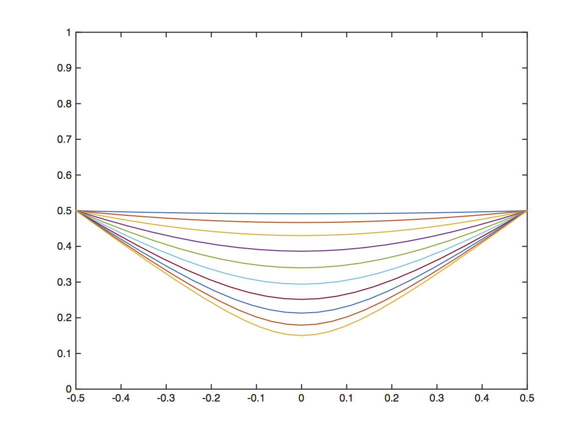
Figure 4: Periodic motions in normalized variables for several values of $T$, orientation of the final velocity is defined by $0<-\frac{\dot{Y}_{0}}{\dot{X}_{0}}<1$.

In [6], it is shown that for a periodic motion of the LIP, self-stabilization is impossible. In this section, our objective is to show the influence of the virtual constraints chosen for the swing leg, and especially the influence of the switching manifold on the self-synchronization of the walking gait. Indeed, since synchronization between the sagittal and frontal motions implies coupling between these two motions and since these motions are decoupled during the single support phase, it is essential to introduce a coupling at the transition.

For the 3D LIP model, due to the specific values of $X_{0},X_{f},Y_{0},Y_{f}$, the switching configuration manifold corresponding to the virtual constraints defined in (36) becomes:

$$\mathbb{S}=\left\{(X,Y)|X^{2}+CY^{2}-(X_{0}^{2}+CY_{0}^{2})=0\right\}$$ (44)

because $X_{a}=0$ using (35) with (43).

The virtual constraints for the swing legs are also designed such that $(X^{+},Y^{+})=(X_{0},Y_{0})$ at the beginning of the ensuing step, so the 3D LIP is said to be $(X_{0},Y_{0})$-invariant. In scaled coordinates, we limit our study to the case $X_{0}=-\frac{1}{2}$ and $Y_{0}=\frac{1}{2}$.

For an $(X_{0},Y_{0})$-invariant 3D LIP, if the switching manifold is defined by (44), reference [26] shows that the Jacobian of the Poincaré return map at the fixed point, expressed in the coordinate system $(X_{k}^{-},\mathcal{L}_{k},\mathcal{K}_{k}^{-})$, where $\mathcal{L}_{k}$ is the synchronization measure at the end of step $k$ and $\mathcal{K}_{k}^{-}$ is the kinetic energy at the end of the step $k$, is in the form

$$\mathbf{J}=\begin{bmatrix}0&*&0\\ 0&-\lambda_{\mathcal{L}}&0\\ 0&*&1\end{bmatrix},$$ (45)

where $*$ represents non-zero terms. Three eigenvalues are identified in this Jacobian. One is zero due to the fact that the position of the CoM at the end of one step does not affect the dynamics of the following step for an $(X_{0},Y_{0})$-invariant 3D LIP. One is a unit eigenvalue which corresponds to the kinetic energy of the pendulum, which indicates that a variation of the kinetic energy will be conserved, and the system will not converge to its original fixed point.

We will propose in this paper a new expression for $\lambda_{\mathcal{L}}$, and we will give an original condition on the choice of the switching manifold to induce synchronization and a physical interpretation of this condition.

Suppose that the state of the robot is slightly perturbed around the initial periodic state: $[-1/2,1/2,\dot{X}_{0},\dot{Y}_{0}]$. After $i$ steps the initial state of the robot is denoted by $[-1/2,1/2,\dot{X}_{i},\dot{Y}_{i}]$, and its synchronization measure is denoted $L_{i}$. After the following step the state will be $[-1/2,1/2,\dot{X}_{i+1},\dot{Y}_{i+1}]$, and its synchronization measure is denoted by $L_{i+1}$. The calculation of ${\frac{L_{i+1}}{L_{i}}}$ is developed in the appendix. The derivation is based on the conservation of orbital energies (41), the synchronization measure (42) during a single support phase, and the fact that the change of support occurs on the switching manifold (44). For small variation around the periodic orbit, the final error for each step satisfies:

$$\delta X^{-}_{i}=-C\delta Y^{-}_{i}.$$ (46)

Direct calculation gives:

$$\lambda_{\mathcal{L}}=\lim_{i\rightarrow\infty}{\frac{L_{i+1}}{L_{i}}}=\frac{(\dot{Y}_{0}-\dot{X}_{0})(C\dot{Y}_{0}+\dot{X}_{0})}{(\dot{X}_{0}+\dot{Y}_{0})(-C\dot{Y}_{0}+\dot{X}_{0})}$$ (47)

Two factors appear in (47): one varies as a function of $C$ and can be modified by the design of the switching manifold, while the other depends on the periodic gait velocity, i.e on the step duration of the gait.

When $C\dot{Y}_{0}+\dot{X}_{0}=0$, the synchronization occurs in one step. This case corresponds to a switching line co-linear with the initial velocity of the periodic motion since in this case we have:

$$C=-\frac{\delta X^{-}_{i}}{\delta Y^{-}_{i}}=-\frac{\dot{X}_{0}}{\dot{Y}_{0}}$$ (48)

Thus, the cross product between the final error in position $(\delta X^{-}_{i},\delta Y^{-}_{i})$ and initial periodic velocity $(\dot{X}_{0},\dot{Y}_{0})$ is zero.

The values of $C$ that ensure synchronization of the motion must be such that:

$$\left|\lambda_{\mathcal{L}}\right|=\left|\frac{(\dot{Y}_{0}-\dot{X}_{0})(C\dot{Y}_{0}+\dot{X}_{0})}{(\dot{X}_{0}+\dot{Y}_{0})(-C\dot{Y}_{0}+\dot{X}_{0})}\right|<1$$ (49)

For a periodic velocity corresponding to Figure 4, namely, when $\dot{X}_{0}>0$, $\dot{Y}_{0}<0$, $\dot{X}_{0}>-\dot{Y}_{0}$, it can be shown that $C$ has to satisfy:

$$1<C<\left(\frac{\dot{X}_{0}}{\dot{Y}_{0}}\right)^{2}.$$ (50)

In Figure 5, for the same initial state, the behavior of the LIP is shown for several values of C. Three cases are illustrated for C satisfying (50) or not. For $C=0.95$, since condition (50) is not satisfied, a periodic motion is not obtained, and the direction of walking is not along the axis $s_{0}$. For the two other cases tested, the condition (50) is satisfied, and convergence to a periodic motion is observed, but in the two cases, the periodic gait velocities differ. In the case $C=1.45$, since the value of $C$ is close to (48), the synchronization is faster than in the case $C=1.2$. It should be noted that the values of $\dot{X}_{0},\dot{Y}_{0}$ correspond to the periodic motion. In the case $C=1.2$, the LIP motion converges to a motion such that $\dot{X}_{0}=2.3265~{}s^{-1}$, $\dot{Y}_{0}=-1.5059~{}s^{-1}$, thus, $-\frac{\dot{X}_{0}}{\dot{Y}_{0}}=1.5449$. In the case $C=1.45$, the LIP motion converges to a motion such that $\dot{X}_{0}=2.2639~{}s^{-1}$, $\dot{Y}_{0}=-1.5476~{}s^{-1}$, thus, $-\frac{\dot{X}_{0}}{\dot{Y}_{0}}=1.4628$.

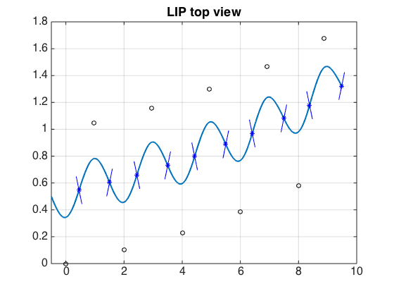
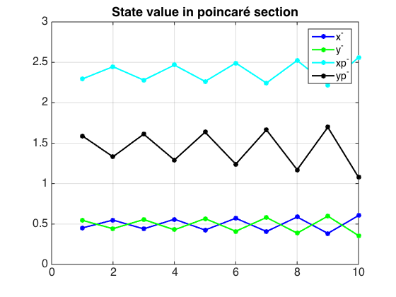
Figure 5: Starting from the same initial state $X_{0}=-0.5$, $Y_{0}=0.5$, $\dot{X}_{0}=2.3147~{}s^{-1}$, $\dot{Y}_{0}=-1.5136~{}s^{-1}$, the simulation of 10 steps shows several behaviors depending on the switching manifold defined by $C$. From top to bottom, we have $C=0.95$; $C=1.2$, $C=1.45$. The left-hand figures show the position of the stance foot, the evolution of the CoM, and a part of the switching manifold are shown. On the right-hand figures, the state of the HZD is shown in the Poincaré section, just before the change of support: divergence or convergence is clearly illustrated.

In Figure 6 the level contours of $|\lambda_{\mathcal{L}}|$ are drawn as a function of the parameter $C$ and the step duration $T$.

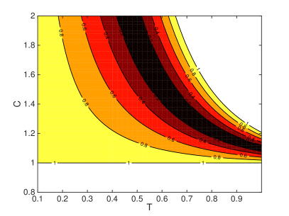
Figure 6: $\lambda_{\mathcal{L}}$ level contours expressed as function of $C$ and step duration $T$ for the LIP model and $z_{0}=0.7$ m.

The condition $|\lambda_{\mathcal{L}}|<1$ ensures convergence toward a synchronized motion, thus is a condition of self-synchronization. However, the walking velocity of the gait is not controlled in the sense that a perturbation of such a gait will result in the convergence of the gait back to a periodic motion, but with a different gait velocity as illustrated in Figure 5. In the next section, we will see how judiciously adding oscillations of the CoM can stabilize the walking velocity.

IV-D VLIP model and self-stabilization

From study of planar walking robots, it is known that vertical oscillations of the CoM can asymptotically stabilize a periodic walking gait [32]. Thus, here, in order to stabilize the walking velocity in an $(X_{0},Y_{0})$-invariant gait, oscillations of the CoM will be introduced. These oscillations of the CoM are obtained by the following virtual constraint:

$$z^{d}(X,Y)=z_{0}-aS_{a}(X,Y),$$ (51)

with $S_{a}(X,Y)$ defined in (34) associated to the ellipse-shaped switching manifold defined in (36)

The expression of $S_{a}$ ensures that at the beginning and end of the step $z^{d}=z_{0}$ since $S_{a}(X_{0},Y_{0})=S_{a}(X_{f},Y_{f})=0$. Note that the case $a=0$ with $X_{a}=0$ corresponds to the 3D LIP example described in Section IV-C.

During the single-support phase, the horizontal position of the mass is located inside the ellipse; thus, $S_{a}(X,Y)$ is negative and increasing when approaching the switching manifold ellipse. Choosing $a>0$ will ensure a negative vertical velocity of the mass at the transition (see Figure 7).

Figure 7: Surface defined by the virtual constraint for the vertical motion the mass motion $z^{d}(X,Y)$. The red curve gives an example of the mass evolution during a single support phase.

This negative vertical velocity of the CoM right before the change of support implies that the angular momenta $\sigma_{X}$ and $\sigma_{Y}$ decrease at the change of support. In order to obtain a periodic motion, the angular momenta must therefore increase during the stance phase, and thus it is necessary to slightly shift the relative position of the support leg and the CoM [5]. The position of the CoM at the beginning of the step is then written as $X_{0}=-\frac{1}{2}+D_{X}$, $Y_{0}=\frac{1}{2}-D_{Y}$ and at the end of the step $X_{f}=\frac{1}{2}+D_{X}$, $Y_{f}=\frac{1}{2}+D_{Y}$ with $D_{X}=\frac{X_{0}+X_{f}}{2}\geq 0$ and $D_{Y}=\frac{Y_{f}-Y_{0}}{2}\geq 0$.

This choice of the switching manifold only ensures the continuity of the vertical position of the CoM. To ensure the continuity of the vertical velocity of the CoM as well, a third order polynomial function of $X$, denoted by $z_{cor}(X)$, is added to expression (51) for $z^{d}$. This function is null at the beginning of the step, where $X=X^{+}$, because the continuity of the position is already ensured, but its derivative should compensate the difference between the vertical velocity at the end of the previous step and the one corresponding to the reference $\dot{z}^{d}(X_{0},Y_{0})$ in (51). This correction term only acts from the beginning of the step where $X=X^{+}$ to the mid-step where $X=D_{X}$. In the second half of the step, where $X\geq D_{X}$, $z_{cor}(X)\equiv 0$, and smoothness in the mid-step is guaranteed by imposing the conditions $z_{cor}(D_{X})=\dot{z}_{cor}(D_{X})=0$. This technique, which has already been used in previous studies [22, 7], is illustrated in Figure 8.

Figure 8: Planar illustration of the modification of the virtual constraint at the beginning of each step to avoid discontinuity in tracking error. At the beginning of the step, the virtual constraint, in black, is continuous for the height of the CoM, but the velocity is not continuous. A modification of the virtual constraint $z_{cor}(X)$ is added to satisfy the conditions of continuity, the constraint effectively used is shown in red.

In the presence of vertical oscillations, periodic motions will exist only for an appropriate set of virtual constraints. In particular, the values of $D_{X}$ and $D_{Y}$ cannot be chosen arbitrarily. In practice, the values of $C$, $a$, and $T$, the duration of the periodic step, are chosen, and $D_{X}$, $D_{Y}$, and the angular momentum at the end of the single support (or the final velocity of the CoM $(\dot{X}^{+}$, $\dot{Y}^{+}$) are deduced by solving a boundary value problem describing the periodicity of the evolution of the CoM. The variations of $D_{X}$ and $D_{Y}$ as functions of $a$ for fixed values of $C$ and $T$ are shown in Figure 9(b).

IV-E Stability of the gait obtained

The study of the gait stability is undertaken through numerical calculations. The evolution of the mass in single support is integrated numerically from the dynamic model (30) taking into account the conditions (51) and (36) developed in Section IV.

To study the effect of oscillations on stability, we first revisit the 3D LIP case ($a=0$). The virtual constraints are completely defined by the value of $z_{0}$ and $C$. We fix $z_{0}=0.7~{}m$ and will study the effect of the parameter $C$. Many periodic orbits exist for $a=0$ corresponding to various step durations $T$, however, for a given value of $T$, a unique periodic gait exists. As explained in Section IV-C, three eigenvalues are evaluated to examine the stability of the periodic motion. In our numerical study, the Poincaré return map is expressed using our state variables $\boldsymbol{\chi}_{k}$. Because the eigenvalues of the Jacobian of the Poincaré map are invariant under a change of coordinates, the results that we observed are identical to those of (45): among the three eigenvalues, one is equal to zero, one is equal to 1, and the last one is $\lambda_{\mathcal{L}}$. Selecting $C$ and step duration $T$ such that $|\lambda_{\mathcal{L}}|<1$ according to (50) will allow us to observe the effect of oscillations on the eigenvalues. Figure 9(a) illustrates the evolution of the three eigenvalues $e_{1},e_{2}$, and $e_{3}$ for $C=1.1$ and $T=0.7$ s as the oscillation amplitude parameter $a$ increases. In our example, the magnitudes of the two non-null eigenvalues decrease as the amplitude of the oscillations increases. Thus, when $a>0$, the absolute values of all eigenvalues are smaller than 1. Consequently, we observe that introducing oscillations transforms the self-synchronization property of the walking gait into self-stabilization. Figure 10 shows the effect of oscillations on stability; the stability criterion $\delta$ (defined as the maximum magnitude of the eigenvalues) is shown via level contours for several values of the ellipse parameter $C$ and a given step duration $T=0.7$ s. The value $\delta$ decreases when $a$ increases. We observe that when oscillations are introduced, the values of the ellipse parameter $C$ for which stability exists are close to the ones where self-synchronization is observed for the 3D LIP. Figure 11 shows the evolution of the stability criterion $\delta$ for $a=0.02$ m. We can see that the stability effect observed in our first example (Figure 9(a)) is extended to most of the values of the parameter $C$ and step duration $T$.

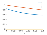
(a)

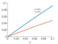
(b)

Figure 9: Influence of the amplitude of vertical oscillation characterized by $a$ on the stability via the magnitude of the three eigenvalues $e_{1},e_{2},e_{3}$ (a) and on the support foot position shift (b). Illustrations are numerically obtained for the case $z_{0}=0.7$ m, $C=1.1$ and $T=0.7$ s.

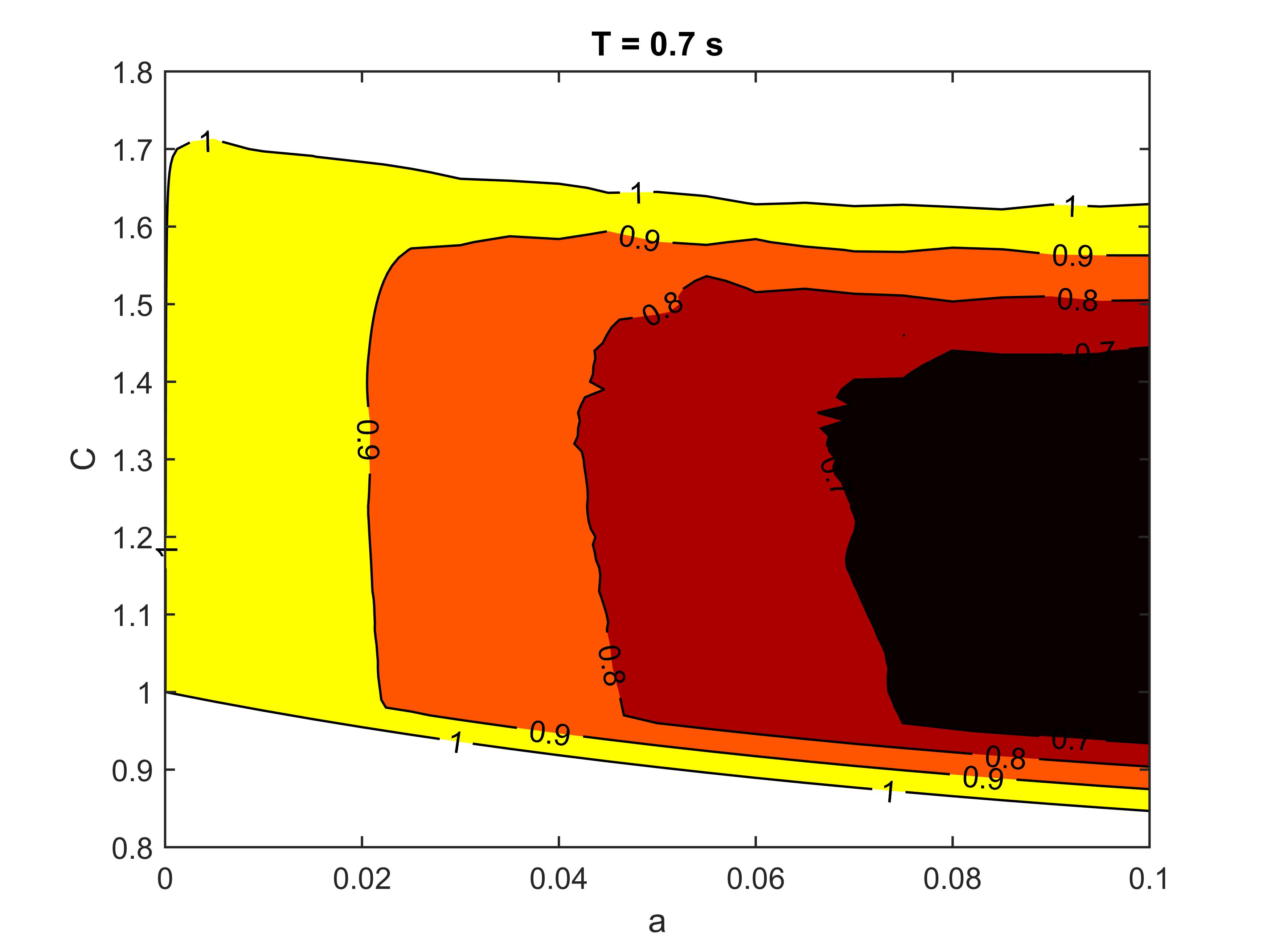
Figure 10: Stability criterion level contours for the pendulum model as function of $C$ and amplitude parameter $a$ for $T=0.7$ s and $z_{0}=0.7$ m.

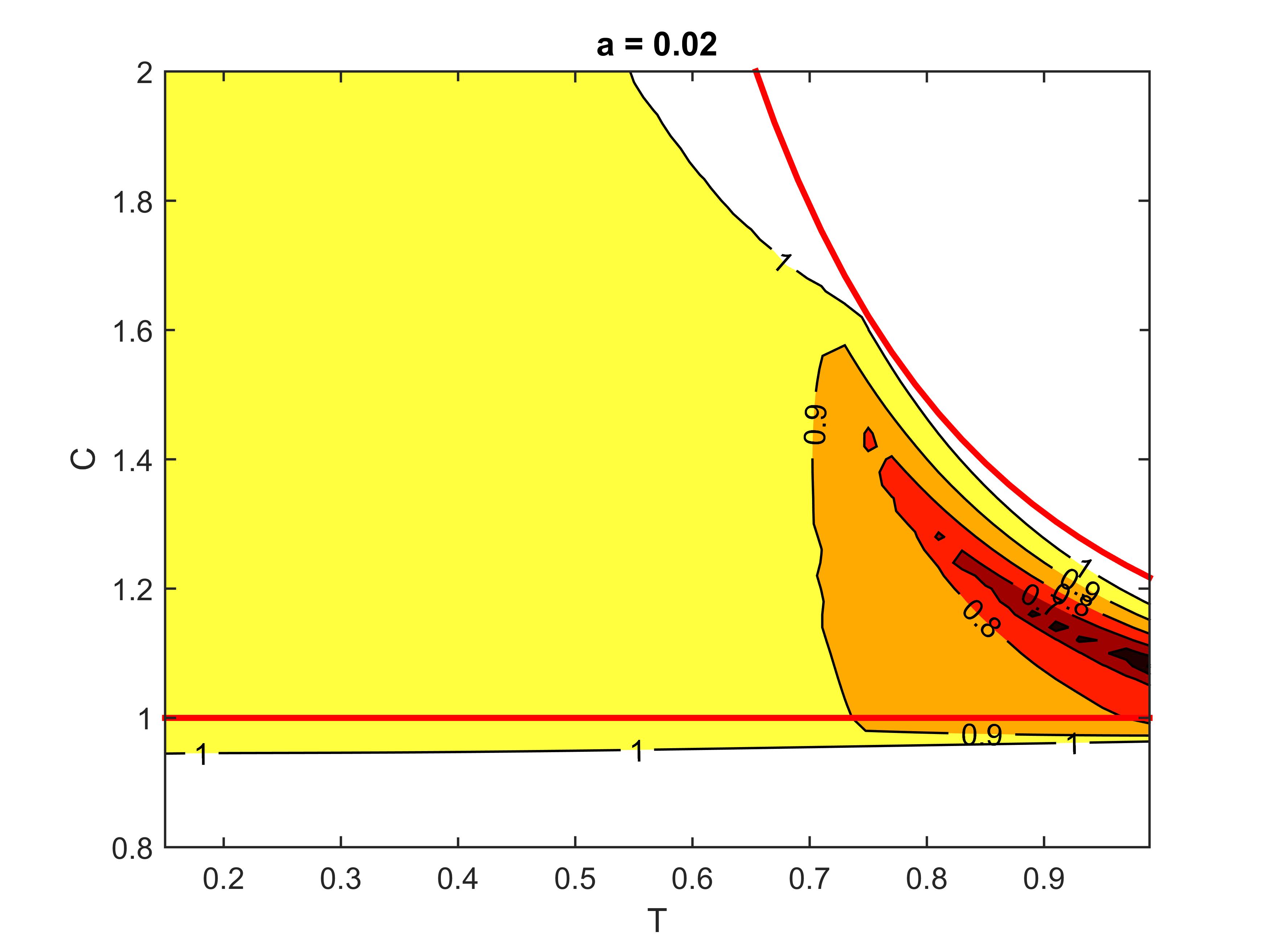
Figure 11: Stability criterion level contours for the pendulum model as function of $C$ and step duration $T$ for $a=0.02$ m and $z_{0}=0.7$ m. The red curves represent the boundaries inside which $|\lambda_{\mathcal{L}}|<1$ (equation (50)) for the LIP.

To complete this analysis, Figure 9(b) shows the evolution of the parameters $D_{X}$ and $D_{Y}$, which introduce asymmetry in the gait, obtained for a periodic motion as the amplitude of the oscillations increases. As expected, the values of $D_{X}$ and $D_{Y}$ increase with oscillations to compensate the loss of angular momentum at the support change.

Figure 12 illustrates the evolution of the CoM in the horizontal, sagittal, and frontal planes for several step durations with $a=0.02$ m. A figure-eight-shaped evolution of the CoM can be observed in the frontal plane, which is qualitatively similar to the motion of the CoM of a human during walking [10].

Figure 12: Motion of the mass in horizontal (a), sagittal (b), and frontal (c) planes ($a=0.02$, $C=1.1$, $z_{0}=0.7$). Magenta, cyan, black, and black have periods of $T=0.5\text{ s},T=0.7\text{ s},T=0.9\text{ s}$, and $T=1\text{ s}$, respectively. Green dots are initial positions and red dots final positions for one step.

V Extension to the control of a humanoid robot model

We saw in Section IV-E that by introducing oscillations of the CoM and with an appropriate change of support, it is possible to generate asymptotically stable periodic walking gaits for the inverted pendulum model. In this section, we apply the same principles to a more complex model of a bipedal robot. In particular, we consider a general $n$-DoF humanoid robot with six joints per leg, where link mass parameters and actuator inertias are taken into account. Numerical simulation will then allow us to discuss the similarities and differences between this complex model and the simple inverted pendulum with variable leg length which was studied in Section IV-D. Indeed, the simulations will confirm that an asymptotically stable periodic gait can be achieved for the complex model.

To illustrate our method of generating stable periodic walking gaits, we study the robot Romeo [23], [27, Chapter  7], which is a 31-DoF humanoid robot constructed by SoftBank Robotics (https://www.ald.softbankrobotics.com/fr/cool-robots/romeo). Similar to the pendulum model, the numerical study will focus on the effects of:

• the transition condition from step to step as defined by the $C$ parameter of the switching manifold defined in (34); and

• vertical oscillations of the CoM as defined by the parameter $a$.

V-A A periodic walking gait for the humanoid robot Romeo

As we would like to reproduce the results obtained for the pendulum, the same virtual constraints used previously and summarized here will be used:

• The height of the center of mass is given by:

  $$\begin{array}[]{ccc}z^{d}&=&z_{0}-aS_{a}(X,Y)+P(X)~{}\mathrm{for}~{}X<DX,\\ z^{d}&=&z_{0}-aS_{a}(X,Y)~{}\quad\quad\quad\quad\mathrm{for}~{}X\geq DX\end{array}$$ (52)

• The height of the swing foot is given by:

  $$\begin{array}[]{ccc}z_{s}^{d}&=&\nu_{z}S_{a}(X,Y),+P_{z}(X)~{}\mathrm{for}~{}X<DX,\\ z_{s}^{d}&=&\nu_{z}S_{a}(X,Y)~{}\quad\quad\quad\quad\mathrm{for}~{}X\geq DX\end{array}$$ (53)

• The horizontal position of the swing foot is given by:

  $$\begin{array}[]{lr}X_{s}^{d}=\left(1-\nu_{X}S_{a}(X,Y)\right)\left(1/2-D_{X}+X\right)+P_{x}(X)&\\ ~{}\quad\quad\quad\quad\quad\quad\quad\quad\quad\quad\quad\quad\quad\quad\quad\quad\quad\mathrm{for}~{}X<X^{l},\\ X_{s}^{d}=\left(1-\nu_{X}S_{a}(X,Y)\right)\left(1/2-D_{X}+X\right)\mathrm{for}~{}X\geq X^{l}.\\ Y_{s}^{d}=\left(1-\nu_{Y}S_{a}(X,Y)\right)\left(1/2+D_{Y}+Y\right)+P_{y}(X)\\ ~{}\quad\quad\quad\quad\quad\quad\quad\quad\quad\quad\quad\quad\quad\quad\quad\quad\quad\mathrm{for}~{}X<X^{l},\\ Y_{s}^{d}=\left(1-\nu_{Y}S_{a}(X,Y)\right)\left(1/2+D_{y}+Y\right)~{}\mathrm{for}~{}X\geq X^{l}.\end{array}$$ (54)

with $S_{a}(X,Y)=(X-D_{x}-CD_{y})^{2}+CY^{2}-((-1/2-CD_{y})^{2}+C(1/2+D_{Y}^{2})$.

Here, for simplicity, the remaining DoFs are fixed to realistic constant values. The orientation of the swing foot is controlled to be constant (the foot remains flat with respect to the ground). The upper-body joints are constrained to fixed positions and the orientation of the torso is controlled to be zero (in each of its Euler angles). The fixed upper-body configuration is visible in Figure 13. While the chosen values may have an influence over the gait stability, examining their potential effects is out of the scope of this study.

In contrast to the simple pendulum model, it is necessary to take into account the step length and width in the design of the constraints due to limits in the robot’s workspace and because the motion of the swing leg affects the dynamics of the robot. Here, we study a fixed step length $S=0.3~{}m$ and width $D=0.15~{}m$.

The periodic motion of the robot is imposed by the parameters defining the virtual constraints and the HZD model (23). Part of the parameters are chosen arbitrarily, and some parameters are defined by optimization to guarantee the existence of a periodic motion compatible with the under-actuation of the robot satisfying some constraints such as duration of the step. Table I defines the chosen parameters and their effect, while Table II presents the optimized parameters.

	Value	Effect
a	several	amplitude of oscillations of CoM
C	several	shape of the switching manifold
T	several	duration of the single support
$z_{0}$	0.65 m	minimal high of the CoM
$\nu_{z}$	0.09 m (0.045 m)	maximal high of the swing foot
$X^{l}$	$0.4+D_{X}$	limit to adapt the horizontal
		motion of the swing foot

TABLE I: The fixed parameters

	Effect
$D_{X}$	shift of the CoM position along axis x
$D_{Y}$	shift of the CoM position along axis y
$\nu_{x}$	such that the horizontal velocities of
$\nu_{y}$	the swing leg tip are null at the end of SS

TABLE II: The optimized parameters

An example of a walking gait obtained for the robot is illustrated in Figure 13. In this example, $C=1$, $T=0.55~{}s$, and $a=0.05~{}m$. A periodic orbit of the system is found by calculating a fixed point of the Poincaré return map. Here we have $D_{X}=0.0016$, $D_{Y}=0.0259$, $\sigma_{X}^{-}=20.48~{}kg.m.s^{-1}$, and $\sigma_{Y}^{-}=-6.9~{}kg.m.s^{-1}$.

From the obtained periodic orbit we observe that the range of motion of the CoM in the frontal plane is relatively small. Moreover, the obtained walking gait is highly dynamic as the angular momentum in the sagittal plane is relatively high, which on the other hand, makes a small initial velocity insufficient for initiating the walking gait.

We notice that when the walking velocity decreases, the amplitude of the lateral motion of the CoM increases, and the workspace limitation for the leg prevents finding a periodic motion for the chosen value of $z_{0}$.

Figure 13: A periodic motion obtained with the proposed approach for $C=1$, $T=0.55~{}s$, $a=0.05~{}m$

V-B Stability of walking

Our main objective is to discover to what extent the effects of $C$ and $T$ on the stability of walking for a pendulum model can be extrapolated to the stability of walking of a realistic humanoid. Figure 14 shows the evolution of the stability criterion (maximum eigenvalue magnitude of the Jacobian of the Poincaré return map) as a function of $C$ and $T$ for vertical oscillations with $a=0.03~{}m$. We observe that the shape of the stable area as a function of parameters $C$ and $T$ is quite similar to the one obtained for the pendulum model but with a shifting of the area of stability toward smaller values of $C$.

Figure 14: Stability criterion level contours for the complete model as a function of $C$ and step duration $T$ for $a=0.03~{}m$, $S=0.3$ m.

V-C Comparison between a realistic and a simplified model

To properly investigate the effect of having a distributed body for the trunk and other links versus having a point mass model, as in the inverted pendulum, we study a simplified model of the robot by concentrating all the mass of the robot to a point of the trunk. This point is placed in a position such that with straight legs, the CoM of the robot and this simplified model coincide. Thus, a model of the robot with similar kinematics but a different mass distribution is considered. The stable area as a function of $C$ and $T$ is presented in Figure 15. We observe that compared to the stability regions of the realistic model of Romeo, which are shown in Figure 14, there is a shifting of the stability areas along the $C$-axis and a slight modification of the stability margin. Aside from these differences, the stability regions for the two models appear quite similar.

Figure 15: Stability criterion level contours for the simplified model of Romeo, where a point mass replaces the distributed mass, as functions of $C$ and step duration $T$ for $a=0.03~{}m$, $S=0.3~{}m$.

As a conclusion, the analysis of the ideal model seems to be an appropriate tool to understand the key features leading to a stable gait, but in order to be able to implement the control laws in practice, studying a more realistic model, like the one presented based on virtual constraints and HZD, is essential to obtain appropriate numerical values for the key parameters.

V-D Effect of the Impact

A main difference between the pendulum model and the complete humanoid model is the impact effect at support change. In the pendulum model, as the legs are massless, no impact is transmitted to the CoM when changing the support leg. Thus, the contact of the swing leg with ground does not affect the pendulum motion. In the complete robot model, however, legs masses are considered, and a rigid impact is modeled as the swing leg touches the ground. This impact has a direct effect on the vertical velocity of the CoM of the humanoid robot when changing support and thus on the stability of the gait [26]. More specifically, loss of kinetic energy at the transition between two steps due to the impact or reduction of angular momentum at the transition [6] may result in stable gaits. To illustrate the contributions of these two mechanisms on stability, the stable areas as functions of $C$ and $T$ are demonstrated in Figure 16. It can be clearly seen that an increase of the vertical oscillations via parameter $a$ leads to an expansion of the stable area and a reduction of the maximal eigenvalue. It can be noted that for a value of $a=0.05~{}m$, the real vertical oscillations of the CoM is only around $0.02~{}m$ as it can be seen in Figure 20. In Figure 16, it is also clear that when the impact is reduced, via a reduction of the vertical velocity of the swing leg tip (induced by a reduction of the height of the swing leg motion right before impact), the area corresponding to the stable motion shrinks and the maximal eigenvalue increases. In the case studied, the horizontal velocity of the swing leg tip at impact is chosen to be null.

Figure 16: Stability criterion level contours for the complete model as function of $C$ and step duration $T$ for several amplitudes of oscillations and impacts. For top to down, the amplitude of oscillations increases $a=0.01~{}m$; $a=0.03~{}m$; $a=0.05~{}m$. From left to right, the amplitude of impact is divided by 2.

V-E Simulation of the walking gait

To illustrate the robustness of the proposed approach with respect to the configuration and velocity of the robot, this section presents some different results obtained with the complex model of the humanoid robot. Starting from rest, the first desired gait corresponds to a walking gait with $S=0.3~{}m$, $D=0.15~{}m$, and $T=0.7~{}s$ for 30 steps, and then a transition to a faster walking gait is imposed with $T=0.55~{}s$ and the same step sizes for 30 others steps.

The robot starts its motion in double support with the two legs in the same frontal plane. In double support, an initial forward motion of the CoM allows the humanoid to increase its angular momentum around the axis $\mathbf{n}_{0}$ such that the barrier of potential energy can be overcome during the first step. This initial motion places the CoM in front of the ankle axis and laterally closer to the next stance foot. This choice of the CoM position at the beginning of the single support is such that during the first single support phase the contribution of gravity to the dynamics will be coherent with the evolution expected during the periodic motion. Based on this initial state, the virtual constraints are built as presented in Section IV-B. The initial configuration of the robot and a representation of the first steps in the sagittal plane are shown in Figure 17, where the schematic of the robot is presented at each transition with the trace of the swing leg tip and the CoM motions.

Figure 17: Illustration of the first steps of the ROMEO gait starting from double support.

The convergence of the solution to the desired periodic orbit can be illustrated in various ways. In Figure 18, the evolution of the state error for the unactuated variables (defined by the difference between the current state and the one corresponding to the desired periodic motion) are shown; the convergence of the error to zero is clear. It can be observed that the convergence to the periodic motion is faster for the first motion (with $T=0.7~{}s$) compared to the second one ($T=0.55~{}s$). This result is coherent with the value of the maximal eigenvalue for the two cases illustrated in Figure 16.

We notice that a faster convergence can be obtained for the error on position than for the error on angular momentum (or velocity). This can be interpreted as a fast synchronization between the motion in the frontal and sagittal planes followed by a stabilization to the desired motion in terms of velocity. This interpretation is reinforced by observing the evolution of the CoM in a frame attached to the stance foot as presented in Figure 19, where the evolutions corresponding to the first four steps are numbered. It can be observed that since the swing leg touches the ground with an imposed distance with respect to the position of the CoM, the initial position of the CoM at the consecutive steps is constant (except for the first step). During the first steps a synchronization is observed due to the choice of the transition between steps as shown in section IV-C. Then there is a slower convergence toward the excepted periodic motion while synchronization is conserved.

We note that even though in the two periodic motions corresponding to $T=0.7~{}s$ and $T=0.55~{}s$ the CoM travels the same distance in the sagittal plane with $S=0.3~{}m$, the distances travelled by the CoM in the frontal plane by the CoM are different.

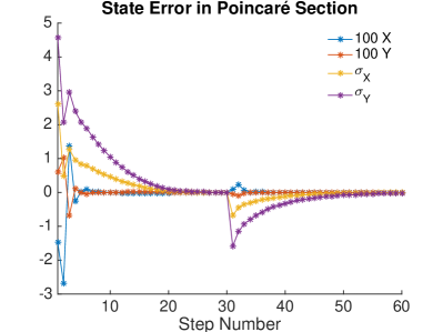
Figure 18: The convergence toward the desired periodic gait is illustrated via the errors on the unactuated state $X,Y,\sigma_{X},\sigma_{Y}$ in the Poincaré section as function of the step number. Due to the scale used, the errors in position are multiplied by $100$ on the graphic.

Figure 19: The evolution of the CoM of the robot in shown in a top view in a frame attached to the stance leg and lateral axis directed toward the CoM. Each step starts with the desired initial position of the CoM. The first steps are numbered, and illustrate a self-synchronization of the walking gait as observed in [26] then the convergence toward the desired motion is obtained. The green and red curves correspond respectively to the desired motions with $T=0.7~{}s$ and $T=0.55~{}s$.

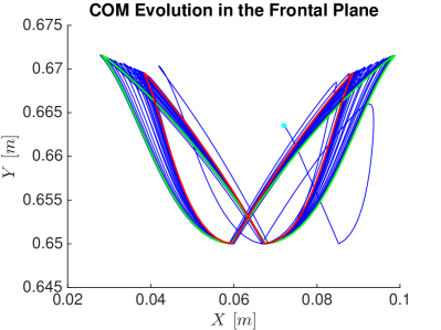
Figure 20: The convergence is shown for the evolution of CoM in a frontal view in a fixed frame. Starting for the state denoted by a cyan star, the motion converge toward the green curve corresponding to the periodic motion with $T=0.7~{}s$ and then to the red curve corresponding to periodic motion with $T=0.55~{}s$.

The evolution of the CoM drawn in the frontal plane in a fixed world frame is shown in Figure 20. It can be noticed that the vertical oscillation of the CoM is limited to approximately $0.02~{}m$ for $a=0.05~{}m$; this amplitude is less than the value observed in human walking.

We can also observe that while the walking gait starts with a foot placed on the point $(0,0,0)$ in a fixed world frame, and the desired distance between feet in the frontal plane is $D=0.15~{}m$, the mean value of the lateral oscillations of the CoM for the last steps is different from $D/2$ (see Figure 20). This can be explained by a step width and length that can be slightly different from $S$ or $D$ during the transient phases. A correction of the path followed can be easily obtained based on [28].

The convergence toward the desired motion is also illustrated in Figure 21 for the motion of one joint (the knee) described in its phase plane and for the evolution of the duration of the step versus the step number.

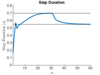
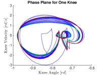
Figure 21: The convergence is shown for the duration of the steps as function of the number of steps in (a) and by the evolution of one knee motion drawn in its phase plane (a). Starting for the state denoted by a cyan star, the motion converges toward the green curve corresponding to the periodic motion with $T=0.7~{}s$ and then to the red curve corresponding to periodic motion with $T=0.55~{}s$.

VI Conclusions

With a control law based on virtual constraints and a planar robot with one degree of underactuation, it is known that the stability of a walking gait depends only on the periodic orbit itself: if the velocity of the CoM at the end of the single support phase is directed downward, the gait is stable. For a 3D humanoid robot with two degrees of underactuation, the condition of stability of a walking gait no longer depends only on the periodic motion but also on the choice of virtual constraints used to create the walking gait. Moreover, the switching manifold plays a crucial role in the synchronization between motion in the sagittal and frontal planes, and thus on stability.

This paper studied the influence of the horizontal position of the CoM at the transition from one step to the next and of vertical oscillations of the CoM within a step on the inherent stability of a walking gait. Through internal constraints on a simplified two-legged pendulum model, we were able to obtain asymptotically stable periodic gaits. The stability properties emerge from the definition of appropriate virtual constraints. In particular, the walking gait does not require stabilization through high-level control commands.

We were able to transfer these properties to a complete robot model and observe qualitatively similar results. In doing this, we did encounter new dynamic effects due to energy loss associated with impacts at leg swapping in the complete model which was not considered in the simple pendulum model. It has to be noted that even if the principles of the approach tested on the simple model can be transferred to the complex model of the robot, the values of our key parameters $C$ have to be slightly modified to take into account the dynamics of the robot. As a consequence, a study of the Hybrid Zero Dynamics corresponding to the specific robot considered is useful for obtaining stable walking gaits.

Finally, a complete model of a humanoid has many degrees of freedom that were not exploited in this study. Here, the upper body and torso joints have been frozen to arbitrary values. In future work, we can exploit the upper body joints—and especially the orientation of the trunk—to increase the energy efficiency of the gaits. Once this is done, our algorithm will be tested experimentally on the humanoid robot Romeo.

Appendix

The control law in single support

From the definition of the virtual constraints, the output and its derivatives are

$$y =q_{\rm c}-h_{d}(q_{\rm f}),$$ (55)

$$\dot{y} =\dot{q}_{\rm c}-\frac{\partial h_{d}(q_{\rm f})}{\partial q_{\rm f}}\dot{q}_{\rm f},$$ (56)

$$\ddot{y} =\ddot{q}_{\rm c}-\frac{\partial h_{d}(q_{\rm f})}{\partial q_{\rm f}}\ddot{q}_{\rm f}-\frac{\partial}{\partial q_{\rm f}}\left(\frac{\partial h_{d}(q_{\rm f})}{\partial q_{\rm f}}\dot{q}_{\rm f}\right)\dot{q}_{\rm f}.$$ (57)

The control objective is to ensure that the components of the output vector $y$ converge to zero sufficiently rapidly. Let denote $\nu(y,\dot{y})$ such a control law, yielding

$$\ddot{y}=\nu(y,\dot{y}).$$ (58)

A special case could be $\nu(y,\dot{y})=-(\frac{K_{d}}{\epsilon}\dot{y}+\frac{K_{p}}{\epsilon^{2}}y)$ for some $K_{p}$ and $K_{d}$ positive definite and $\epsilon>0$ [22].

In the following, we show how one can obtain the control law (i.e., the actuator torques) ensuring the satisfaction of equation (58).

The joint coordinates, velocities and accelerations of the robot can be expressed as function of controlled and free variables:

$$q =F(q_{\rm c},q_{\rm f}),$$ (59)

$$\dot{q} =\frac{\partial F(q_{\rm c},q_{\rm f})}{\partial q_{\rm c}}\dot{q}_{\rm c}+\frac{\partial F(q_{\rm c},q_{\rm f})}{\partial q_{\rm f}}\dot{q}_{f},$$ (60)

$$\ddot{q} =\frac{\partial F(q_{\rm c},q_{\rm f})}{\partial q_{\rm c}}\ddot{q}_{\rm c}+\frac{\partial F(q_{\rm c},q_{\rm f})}{\partial q_{\rm f}}\ddot{q}_{\rm f}+\Psi(q_{\rm c},q_{\rm f},\dot{q}_{\rm c},\dot{q}_{\rm f}),$$ (61)

where

$$\Psi(q_{\rm c},q_{\rm f},\dot{q}_{\rm c},\dot{q}_{f})=\frac{\partial}{\partial(q_{\rm c},q_{\rm f})}\left(\frac{\partial F(q_{\rm c},q_{\rm f})}{\partial(q_{\rm c},q_{\rm f})}\left[\begin{array}[]{l}\dot{q}_{\rm c}\\ \dot{q}_{\rm f}\end{array}\right]\right)\left[\begin{array}[]{l}\dot{q}_{\rm c}\\ \dot{q}_{\rm f}\end{array}\right].$$

Using equations (57) and (58), it follows that in the closed-loop system, the accelerations of the controlled variables satisfy the equation

$$\ddot{q}_{\rm c}=\frac{\partial h_{d}(q_{\rm f})}{\partial q_{\rm f}}\ddot{q}_{\rm f}+\frac{\partial}{\partial q_{\rm f}}\left(\frac{\partial h_{d}(q_{\rm f})}{\partial q_{\rm f}}\dot{q}_{\rm f}\right)\dot{q}_{\rm f}+\nu(y,\dot{y}),$$ (62)

where $y$ and $\dot{y}$ are computed in (55) and (56). The actuator torques able to achieve this desired closed-loop behavior can be computed based on the dynamic model(2). The torque vector $\Gamma$ allowing the $n-2$ controlled variables to follow the desired closed-loop behavior (62), using (59), (60) (61) and (2), satisfies the following equation:

$$\bar{D}(q_{\rm c},q_{\rm f})J_{r}(q_{\rm c},q_{\rm f})\ddot{q}_{\rm f}+\Omega(q_{\rm c},q_{\rm f},\dot{q}_{\rm c},\dot{q}_{\rm f},\nu(y,\dot{y}))=B\Gamma,$$ (63)

where

$$\bar{D}(q_{\rm c},q_{\rm f}) =D(q)\bigg{|}_{q=F(q_{\rm c},q_{\rm f})},\vskip 12.0pt plus 4.0pt minus 4.0pt$$

$$J_{r}(q_{\rm c},q_{\rm f}) =\frac{\partial F(q_{\rm c},q_{\rm f})}{\partial q_{c}}\frac{\partial h_{d}(q_{\rm f})}{\partial q_{\rm f}}+\frac{\partial F(q_{\rm c},q_{\rm f})}{\partial q_{\rm f}}\vskip 12.0pt plus 4.0pt minus 4.0pt,$$

$$\Omega =\bar{D}(q_{\rm c},q_{\rm f}\bigg{[}\frac{\partial F(q_{\rm c},q_{\rm f})}{\partial q_{\rm c}}$$ (64)

$$\bigg{(}\frac{\partial}{\partial q_{\rm f}}\left(\frac{\partial h_{d}(q_{\rm f})}{\partial q_{\rm f}}\dot{q}_{\rm f}\right)\dot{q}_{\rm f}+\vskip 12.0pt plus 4.0pt minus 4.0pt\nu(y,\dot{y})\bigg{)}$$

$$+\Psi(q_{\rm c},q_{\rm f},\dot{q}_{\rm c},\dot{q}_{\rm f})\bigg{]}+\bar{H}(q_{\rm c},q_{\rm f},\dot{q}_{c},\dot{q}_{\rm f}),\vskip 12.0pt plus 4.0pt minus 4.0pt$$

$$\bar{H}(q_{\rm c},q_{\rm f},\dot{q}_{\rm c},\dot{q}_{\rm f}) =H(q,\dot{q})\bigg{|}_{\begin{array}[]{l}q=F(q_{\rm c},q_{\rm f})\\ \dot{q}=\frac{\partial F(q_{\rm c},q_{\rm f})}{\partial q_{\rm c}}\dot{q}_{\rm c}+\frac{\partial F(q_{\rm c},q_{\rm f})}{\partial q_{\rm f}}\dot{q}_{\rm f}\end{array}}$$ (67)

Multiplying (63) on the left by the full rank matrix

$$\left[\begin{array}[]{c}B^{\perp}\\ B^{+}\end{array}\right],$$

where $B^{+}$ is the pseudo inverse of $B$ and $B^{\perp}$ is a $2\times n$ matrix of rank $2$ such that $B^{\perp}B=0$, results in

$$B^{\perp}\bar{D}(q_{\rm c},q_{\rm f})J_{r}(q_{\rm c},\dot{q}_{\rm f})\ddot{q}_{\rm f}+B^{\perp}\Omega(q_{\rm c},q_{\rm f},\dot{q}_{\rm c},\dot{q}_{\rm f},y,\dot{y}) =0$$ (68)

$$B^{+}\bar{D}(q_{\rm c},q_{\rm f})J_{r}(q_{\rm c},q_{\rm f})\ddot{q}_{\rm f}+B^{+}\Omega(q_{\rm c},q_{\rm f},\dot{q}_{\rm c},\dot{q}_{\rm f},y,\dot{y}) =\Gamma.$$ (69)

It follows that a feedback control law ensuring (58) can be obtained from the following equations

$$\Gamma =B^{+}\bar{D}(q_{\rm c},q_{\rm f})J_{r}(q_{\rm c},q_{\rm f})v+B^{+}\Omega(q_{\rm c},q_{\rm f},\dot{q}_{\rm c},\dot{q}_{\rm f},y,\dot{y})$$ (70)

$$v =-\left(B^{\perp}\bar{D}(q_{\rm c},q_{\rm f}J_{r}(q_{\rm c},q_{\rm f})\right)^{-1}B^{\perp}\Omega(q_{\rm c},q_{\rm f},\dot{q}_{\rm c},\dot{q}_{\rm f},y,\dot{y}).$$ (71)

where $v$ denoted the acceleration $\ddot{q}_{\rm f}$ satisfying the equation (68). This form of the feedback law only requires the inversion of a matrix whose size corresponds to the number of unactuated coordinates, here a 2$\times$2 matrix.

Condition of synchronization for the LIP model

This section details of the condition of synchronization for the LIP model and the proposed control strategy, with the virtual constraints proposed in section IV-B.

The initial state of the robot after step i is written as:

$$X^{+}_{i} = -1/2,$$ (72)

$$Y^{+}_{i} = 1/2$$ (73)

$$\dot{X}^{+}_{i} = \dot{X}_{0}+\delta\dot{X}^{+}_{i}$$ (74)

$$\dot{Y}^{+}_{i} = \dot{Y}_{0}+\delta\dot{Y}^{+}_{i}$$ (75)

Due to the discrete invariance of the control law, there is no error on position. At the end of the step the state of the robot will be denoted

$$X^{-}_{i} = 1/2+\delta{X}^{-}_{i}$$ (76)

$$Y^{-}_{i} = 1/2+\delta{Y}^{-}_{i}$$ (77)

$$\dot{X}^{-}_{i} = \dot{X}_{0}+\delta\dot{X}^{-}_{i}$$ (78)

$$\dot{Y}^{-}_{i} = -\dot{Y}_{0}+\delta\dot{Y}^{-}_{i}$$ (79)

Using the fact that $(\dot{X}_{0}$ and $\dot{Y}_{0})$ and $L_{i}=0$ define a synchronized motion and neglecting the second order terms, we obtain:

$$L_{i}\thickapprox\dot{X}_{0}\delta\dot{Y}^{+}_{i}+\dot{Y}_{0}\delta\dot{X}^{+}_{i}$$ (80)

Since the velocity of the CoM is conserved through change of support for the LIP model:

$$\delta\dot{X}^{+}_{i+1} = \delta\dot{X}^{-}_{i}$$

$$\delta\dot{Y}^{+}_{i+1} = -\delta\dot{Y}^{-}_{i}$$

and $L_{i+1}$ can be expressed as

$$L_{i+1}\thickapprox\dot{X}_{0}\delta\dot{Y}^{+}_{i+1}+\dot{Y}_{0}\delta\dot{X}^{+}_{i+1}$$ (81)

or

$$L_{i+1}\thickapprox-\dot{X}_{0}\delta\dot{Y}^{-}_{i}+\dot{Y}_{0}\delta\dot{X}^{-}_{i}$$ (82)

$$\frac{L_{i+1}}{L_{i}}\thickapprox\frac{-\dot{X}_{0}\delta\dot{Y}^{-}_{i}+\dot{Y}_{0}\delta\dot{X}^{-}_{i}}{\dot{X}_{0}\delta\dot{Y}^{+}_{i}+\dot{Y}_{0}\delta\dot{X}^{+}_{i}}$$ (83)

We will now express the final error in velocity as function of the initial error for the step $i$. The orbital energies, $\mathcal{E}_{x}$ and $\mathcal{E}_{y}$ and synchronization measure $L$ are conserved quantities. Therefore, we have,

$$\left(\dot{X}_{i}^{-}\right)^{2}-\omega^{2}\left(X^{-}_{i}\right)^{2} = \left(\dot{X}_{i}^{+}\right)^{2}-\omega^{2}\left(X^{+}_{i}\right)^{2}$$ (84)

$$\left(\dot{Y}_{i}^{-}\right)^{2}-\omega^{2}\left(Y^{-}_{i}\right)^{2} = \left(\dot{Y}_{i}^{+}\right)^{2}-\omega^{2}\left(Y^{+}_{i}\right)^{2}$$ (85)

$$\dot{X}_{i}^{-}\dot{Y}_{i}^{-}-\omega^{2}X^{-}_{i}Y^{-}_{i} = L_{i}$$ (86)

or

$$\left(\dot{X}_{0}+\delta\dot{X}^{-}_{i}\right)^{2}-\omega^{2}\left(1/2+\delta{X}^{-}_{i}\right)^{2}$$

$$=\left(\dot{X}_{0}+\delta\dot{X}^{+}_{i}\right)^{2}-\omega^{2}/4$$

$$\left(-\dot{Y}_{0}+\delta\dot{Y}^{-}_{i}\right)^{2}-\omega^{2}\left(1/2+\delta{Y}^{-}_{i}\right)^{2}$$

$$=\left(\dot{Y}_{0}+\delta\dot{Y}^{+}_{i}\right)^{2}-\omega^{2}/4$$

$$\left(\dot{X}_{0}+\delta\dot{X}^{-}_{i}\right)\left(-\dot{Y}_{0}+\delta\dot{Y}^{-}_{i}\right)$$

$$-\omega^{2}\left(1/2+\delta{X}^{-}_{i}\right)\left(1/2+\delta{Y}^{-}_{i}\right)=L_{i}.$$

Using these equations and neglecting the second order terms we obtain:

$$\delta\dot{X}^{-}_{i} \thickapprox \frac{\omega^{2}}{2\dot{X}_{0}}\delta{X}^{-}_{i}+\delta\dot{X}^{+}_{i}$$ (87)

$$\delta\dot{Y}^{-}_{i} \thickapprox -\frac{\omega^{2}}{2\dot{Y}_{0}}\delta{Y}^{-}_{i}-\delta\dot{Y}^{+}_{i}$$ (88)

$$\frac{\omega^{2}}{2}\left(\delta{X}^{-}_{i}+\delta{Y}^{-}_{i}\right) \thickapprox \dot{X}_{0}\delta\dot{Y}^{-}_{i}-\dot{Y}_{0}\delta\dot{X}^{-}_{i}-L_{i}.$$

The last equation (LABEL:eq:cons_L_annexe) combines with the previous ones (87) (88) can give us a relation between $\delta{X}^{-}_{i}$, $\delta{Y}^{-}_{i}$ and $L_{i}$.

$$\frac{\omega^{2}}{2}\left(\delta{X}^{-}_{i}+\delta{Y}^{-}_{i}\right)\thickapprox-\frac{\omega^{2}\dot{X}_{0}}{2\dot{Y}_{0}}\delta{Y}^{-}_{i}-\frac{\omega^{2}\dot{Y}_{0}}{2\dot{X}_{0}}\delta{X}^{-}_{i}-2L_{i}$$ (90)

$$\left(1+\frac{\dot{Y}_{0}}{\dot{X}_{0}}\right)\delta{X}^{-}_{i}+\left(1+\frac{\dot{X}_{0}}{\dot{Y}_{0}}\right)\delta{Y}^{-}_{i}\thickapprox-4\frac{L_{i}}{\omega^{2}}.$$ (91)

Equation (91) confirms that synchronized motion occurs with $\delta{X}^{-}_{i}=\delta{Y}^{-}_{i}=0$ and in this case via (87) and (88), we see that the error on velocity is conserved. Now we will write the ratio $\dfrac{L_{i+1}}{L_{i}}$ as function of $C$. The change of support occurs on the switching manifold (36). For small variation around the periodic motion, the final position error for each step satisfies:

$$\delta X^{-}_{i}=-C\delta Y^{-}_{i}.$$ (92)

Using (91), the error in position at the end of the step, can deduced as function of $L_{i}$. We have:

$$\delta{Y}^{-}_{i}\thickapprox-4\frac{L_{i}\dot{X}_{0}\dot{Y}_{0}}{\omega^{2}(-\dot{Y}_{0}C+\dot{X}_{0})(\dot{X}_{0}+\dot{Y}_{0})}.$$ (93)

The others errors can also be deduced:

$$\delta{X}^{-}_{i}\thickapprox 4C\frac{L_{i}\dot{X}_{0}\dot{Y}_{0}}{\omega^{2}(-\dot{Y}_{0}C+\dot{X}_{0})(\dot{X}_{0}+\dot{Y}_{0})}$$ (94)

$$\delta\dot{X}^{-}_{i}\thickapprox 2C\frac{L_{i}\dot{X}_{0}\dot{Y}_{0}}{\dot{X}_{0}(-\dot{Y}_{0}C+\dot{X}_{0})(\dot{X}_{0}+\dot{Y}_{0})}+\delta\dot{X}^{+}_{i}$$ (95)

$$\delta\dot{Y}^{-}_{i}\thickapprox 2\frac{L_{i}\dot{X}_{0}\dot{Y}_{0}}{\dot{Y}_{0}(-\dot{Y}_{0}C+\dot{X}_{0})(\dot{X}_{0}+\dot{Y}_{0})}-\delta\dot{Y}^{+}_{i}$$ (96)

We can then calculate the change of synchronization value step by step, we obtain:

$$\frac{L_{i+1}}{L_{i}}\thickapprox\frac{-\dot{X}_{0}\delta\dot{Y}^{-}_{i}+\dot{Y}_{0}\delta\dot{X}^{-}_{i}}{L_{i}}$$ (97)

Using (87) and (88) equation (97) becomes:

$$\frac{L_{i+1}}{L_{i}}\thickapprox\frac{\dot{X}_{0}\delta\dot{Y}^{+}_{i}+\dot{Y}_{0}\delta\dot{X}^{+}_{i}}{L_{i}}+$$

$$2(C\frac{\dot{Y}_{0}}{\dot{X}_{0}}-\frac{\dot{X}_{0}}{\dot{Y}_{0}})\frac{\dot{X}_{0}\dot{Y}_{0}}{(-\dot{Y}_{0}C+\dot{X}_{0})(\dot{X}_{0}+\dot{Y}_{0})}$$ (98)

With (80) equation can be rewritten (98) as follows:

$$\frac{L_{i+1}}{L_{i}}\thickapprox\frac{(\dot{Y}_{0}-\dot{X}_{0})(C\dot{Y}_{0}+\dot{X}_{0})}{(\dot{X}_{0}+\dot{Y}_{0})(-C\dot{Y}_{0}+\dot{X}_{0})}$$ (99)

VII Acknowledgments

We gratefully acknowledge partial support by ANR Equipex Robotex. The work of J. Grizzle was supported by NSF Awards NRI-1525006 and Inspire-1343720.

References

- [1] K. Akbari-Hamed and J.W. Grizzle. Reduced-order framework for exponential stabilization of periodic orbits on parameterized hybrid zero dynamics manifolds: Application to bipedal locomotion. IFAC journal Nonlinear Analysis: Hybrid Systems (NAHS), 25:227–245, 2017.
- [2] A. D. Ames, K. Galloway, K. Sreenath, and J.W. Grizzle. Rapidly exponentially stabilizing control Lyapunov functions and hybrid zero dynamics. Automatic Control, IEEE Transactions on, 59(4):876–891, 2014.
- [3] C. Byrnes and A. Isidori. Asymptotic stabilization of nonlinear minimum phase systems. 376:1122–37, 1991.
- [4] C. Chevallereau, J. W. Grizzle, and C.-L. Shih. Asymptotically stable walking of a five-link underactuated 3D bipedal robot. 25(1):37–50, 2009.
- [5] Christine Chevallereau, Gabriel Abba, Yannick Aoustin, Franck Plestan, E R Westervelt, Carlos Canudas-de wit, and J W Grizzle. RABBIT : A Testbed for advanced Control Theory. IEEE Control Systems Magazine, pages 57–79, 2003.
- [6] Christine Chevallereau and Yannick Aoustin. Self-stabilization of 3D walking via vertical oscillations of the hip. In International Conference on Robotics and Automation, pages 5088–5093, 2015.
- [7] Christine Chevallereau, J. W. Grizzle, and Ching Long Shih. Asymptotically stable walking of a five-link underactuated 3-D bipedal robot. IEEE Transactions on Robotics, 25(1):37–50, 2009.
- [8] S. Collins, A. Ruina, R. Tedrake, and M. Wisse. Efficient bipedal robots based on passive-dynamic walkers. Science, 307(1082–1085), 2005.
- [9] M. Doi, Y. Hasegawa, and T. Fukuda. 3D dynamic walking based on the inverted pendulum model with two degree of underactuation. 2005 IEEE/RSJ International Conference on Intelligent Robots and Systems, pages 4166–4171, 2005.
- [10] Saunders J. et al. The major determinants in normal and pathological gait. The Journal of Bone and Joint Surgery, 35(3):543–558, 1953.
- [11] B. Griffin and J.W. Grizzle. Walking gait optimization for accommodation of unknown terrain height variations. In American Control Conference, 2015.
- [12] Brent Griffin and Jessy Grizzle. Nonholonomic virtual constraints and gait optimization for robust walking control. The International Journal of Robotics Research, Accepted 2017.
- [13] Jessy.W Grizzle and Christine Chevallereau. Virtual Constraints and Hybrid Zero Dynamics for Realizing Underactuated Bipedal Locomotion. https://arxiv.org/pdf/1706.01127.pdf, 2017.
- [14] D. G. E. Hobbelen and M. Wisse. Swing-leg retraction for limit cycle walkers improves disturbance rejection. IEEE Transactions on Robotics, 24(2):377–389, April 2008.
- [15] Y Hurmuzlu and D B Marghitu. Rigid body collisions of planar kinematic chains with multiple contact points. The International Journal of Robotics Research, 13(1):82–92, 1994.
- [16] Jianjuen J.Hu. Stable Locomotion Control of Bipedal Walking Robots: Synchronization with Neural Oscillators and Switching Control. PhD thesis, Massachusetts Institute of Technology, 2000.
- [17] B.G. Buss K. Akbari-Hamed and J.W. Grizzle. Exponentially stabilizing continuous-time controllers for periodic orbits of hybrid systems: Application to bipedal locomotion with ground height variations. The International Journal of Robotics Research, 35(8):977–999, 2015.
- [18] Shuuji Kajita, Fumio Kanehiro, Kenji Kaneko, Kazuhito Yokoi, and Hirukawa Hirohisa. The 3D Linear Inverted Pendulum Mode : A simple modeling for a biped walking pattern generation. IEEE/RSJ International Conference on Intelligent Robots and System, 4:239–246, 2001.
- [19] T. Koolen, T. de Boer, J. Rebula, a. Goswami, and J. Pratt. Capturability-based analysis and control of legged locomotion, Part 1: Theory and application to three simple gait models. The International Journal of Robotics Research, 31:1094–1113, 2012.
- [20] T. McGeer. Passive dynamic walking. The International Journal of Robotics Research, 9(2), 62–82., 1990.
- [21] T. McGeer. Passive walking with knees. In Proc. 1990 IEEE int. conf. robot. autom. (ICRA), pages 1640–1645, Cincinnati, May 1990.
- [22] Benjamin Morris and Jessy W. Grizzle. Hybrid invariant manifolds in systems with impulse effects with application to periodic locomotion in bipedal robots. IEEE Transactions on Automatic Control, 54(8):1751–1764, 2009.
- [23] N. Pateromichelakis, A. Mazel, M. A. Hache, R. Gelin T. Koumpogiannis, B. Maisonnier, and A. Berthoz. Head-eyes system and gaze analysis of the humanoid robot romeo. In Proc of the 2014 IEEE/RSJ Int. Conf. on Intelligent Robots and System, pages 1374–1379, Chicago, USA, 2014.
- [24] Matthew J. Powell, Wen-Loong Ma, Eric R. Ambrose, and Aaron D. Ames. Mechanics-based design of underactuated robotic walking gaits: Initial experimental realization. In 2016 IEEE-RAS 16th International Conference on Humanoid Robots (Humanoids), pages 981–986, Cancun, Mexico, Nov 15-17 2016.
- [25] Hamed Razavi, Anthony M. Bloch, Christine Chevallereau, and J. W. Grizzle. Restricted Discrete Invariance and Self-Synchronization For Stable Walking of Bipedal Robots. In American Control Conference, pages 4818–4824, July 2015.
- [26] Hamed Razavi, Anthony M. Bloch, Christine Chevallereau, and Jessy W. Grizzle. Symmetry in legged locomotion: a new method for designing stable periodic gaits. Autonomous Robots, 41(5):1119–1142, 2017.
- [27] Seyed Hamed Razavi. Symmetry Method for Limit Cycle Walking of Legged Robots. PhD thesis, The University of Michigan, 2016.
- [28] Ching-Long Shih, J. W. Grizzle, and Christine Chevallereau. From stable walking to steering of a 3d bipedal robot with passive point feet. Robotica, 30(7):119–1130, 2012.
- [29] M.W. Spong and F. Bullo. Controlled symmetries and passive walking. IEEE Transactions on Automatic Control, 50(7):1025–1031, 2005.
- [30] P. van Zutven and H. Nijmeijer. Foot Placement Indicator for Balance of Planar Bipeds with Point Feet. International Journal of Advanced Robotic Systems, 10:1–11, 2013.
- [31] E.R. Westervelt, J.W. Grizzle, and D.E. Koditschek. Hybrid zero dynamics of planar biped walkers. IEEE Transactions on Automatic Control, 48(1):42–56, jan 2003.
- [32] Eric R Westervelt, Jessy W Grizzle, Christine Chevallereau, Jun Ho Choi, and Benjamin Morris. Feedback Control of Dynamic Bipedal Robot Locomotion. CRC Press, 2007.
- [33] Chen. Z., Lakbakbi Elyaaqoubi N., and Abba G. Optimized 3D stable walking of a bipedal robot with line-shaped massless feet and sagittal underactuation. Robotics and Autonomous Systems, 83:203–216, 2016.