Abstract

Discovering causal relations is fundamental to reasoning and intelligence. In particular, observational causal discovery algorithms estimate the cause-effect relation between two random entities $X$ and $Y$, given $n$ samples from $P(X,Y)$.

In this paper, we develop a framework to estimate the cause-effect relation between two static entities $x$ and $y$: for instance, an art masterpiece $x$ and its fraudulent copy $y$. To this end, we introduce the notion of proxy variables, which allow the construction of a pair of random entities $(A,B)$ from the pair of static entities $(x,y)$. Then, estimating the cause-effect relation between $A$ and $B$ using an observational causal discovery algorithm leads to an estimation of the cause-effect relation between $x$ and $y$. For example, our framework detects the causal relation between unprocessed photographs and their modifications, and orders in time a set of shuffled frames from a video.

As our main case study, we introduce a human-elicited dataset of 10,000 pairs of casually-linked pairs of words from natural language. Our methods discover 75% of these causal relations. Finally, we discuss the role of proxy variables in machine learning, as a general tool to incorporate static knowledge into prediction tasks.

1 Introduction

Discovering causal relations is a central task in science (Pearl, 2009; Beebee et al., 2009), and empowers humans to explain their experiences, predict the outcome of their interventions, wonder about what could have happened but never did, or plan which decisions will shape the future to their maximum benefit. Causal discovery is essential to the development of common-sense (Kuipers, 1984; Waldrop, 1987). In machine learning, it has been argued that causal discovery algorithms are a necessary step towards machine reasoning (Bottou, 2014; Bottou et al., 2013; Lopez-Paz, 2016) and artificial intelligence (Lake et al., 2016).

The gold standard to discover causal relations is to perform active interventions (also called experiments) in the system under study (Pearl, 2009). However, interventions are in many situations expensive, unethical, or impossible to realize. In all of these situations, there is a prime need to discover and reason about causality purely from observation. Over the last decade, the state-of-the-art in observational causal discovery has matured into a wide array of algorithms (Shimizu et al., 2006; Hoyer et al., 2009; Daniusis et al., 2012; Peters et al., 2014; Mooij et al., 2016; Lopez-Paz et al., 2015; Lopez-Paz, 2016). All these algorithms estimate the causal relations between the random variables $(X_{1},\ldots,X_{p})$ by estimating various asymmetries in $P(X_{1},\ldots,X_{p})$. In the interest of simplicity, this paper considers the problem of discovering the causal relation between two variables $X$ and $Y$, given $n$ samples from $P(X,Y)$.

The methods mentioned estimate the causal relation between two random entities $X$ and $Y$, but often we are interested instead in two static entities $x$ and $y$. These are a pair of single objects for which it is not possible to define a probability distribution directly. Examples of such static entities may include one art masterpiece and its fraudulent copy, one translated document and its original version, or one pair of causally linked words in natural language, such as “virus” and “death”. Looking into the distant future, an algorithm able to discover the causal structure between static entities in natural language could read throughout medical journals, and discover the causal mechanisms behind a new cure for a specific disease–the very goal of the ongoing $45 million dollar Big Mechanism DARPA initiative (Cohen, 2015). Or, if we were able to establish the causal relation between two arbitrary natural language statements, we could tackle general-AI tasks such as the Winograd schema challenge (Levesque et al., 2012), which are out-of-reach for current algorithms. The above and many more are situations where causal discovery between static entities is at demand.

Our Contributions

First, we introduce the framework of proxy variables to estimate the causal relation between static entities (Section 3).

Second, we apply our framework to the task of inferring the cause-effect relation between pairs of images (Section 4). In particular, our methods are able to infer the causal relation between an image and its stylistic modification in $80\%{}$ of the cases, and it can recover the correct ordering of a set of shuffled video frames (Section 4.2).

Third, we apply our framework to discover the cause-effect relation between pairs of words in natural language (Section 5). To this end, we introduce a novel dataset of 10,000 human-elicited pairs of words with known causal relation (Section 5.2). Our methods are able to recover $75\%{}$ of the cause-effect relations (such as “accident $\to$ injury” or “sentence $\to$ trial”) in this challenging task (Section 5.4).

Fourth, we discuss the role of proxy variables as a tool to incorporate external knowledge, as provided by static entities, into general prediction problems (Section 6).

All our code and data are available at anonymous.

We start the exposition by introducing the basic language of observational causal discovery, as well as motivating its role in machine learning.

2 Causal Discovery in Machine Learning

The goal of observational causal discovery is to reveal the cause-effect relation between two random variables $X$ and $Y$, given $n$ samples $(x_{1},y_{1}),\ldots(x_{n},y_{n})$ from $P(X,Y)$. In particular, we say that “$X$ causes $Y$” if there exists a mechanism $F$ that transforms the values taken by the cause $X$ into the values taken by the effect $Y$, up to the effects of some random noise $N$. Mathematically, we write $Y\leftarrow F(X,N)$. Such equation highlights an asymmetric assignment rather than a symmetric equality. If we were to intervene and change the value of the cause $X$, then a change in the value of the effect $Y$ would follow. On the contrary, if we were to manipulate the value of the effect $Y$, a change in the cause $X$ would not follow.

When two random variables share a causal relation, they often become statistically dependent. However, when two random variables are statistically dependent, they do not necessarily share a causal relation. This is at the origin of the famous warning “dependence does not imply causality”. This relation between dependence and causality was formalized by Reichenbach (1956) into the following principle.

Principle 1 (Principle of common cause).

If two random variables $X$ and $Y$ are statistically dependent ($X\not\perp Y$), then one of the following causal explanations must hold:

• $X$ causes $Y$ (write $X\to Y$), or

• $Y$ causes $X$ (write $X\leftarrow Y$), or

• there exists a random variable $Z$ that is the common cause of both $X$ and $Y$ (write $X\leftarrow Z\to Y$).

In the third case, $X$ and $Y$ are conditionally independent given $Z$ (write $X\perp Y{\,|\,}Z$).

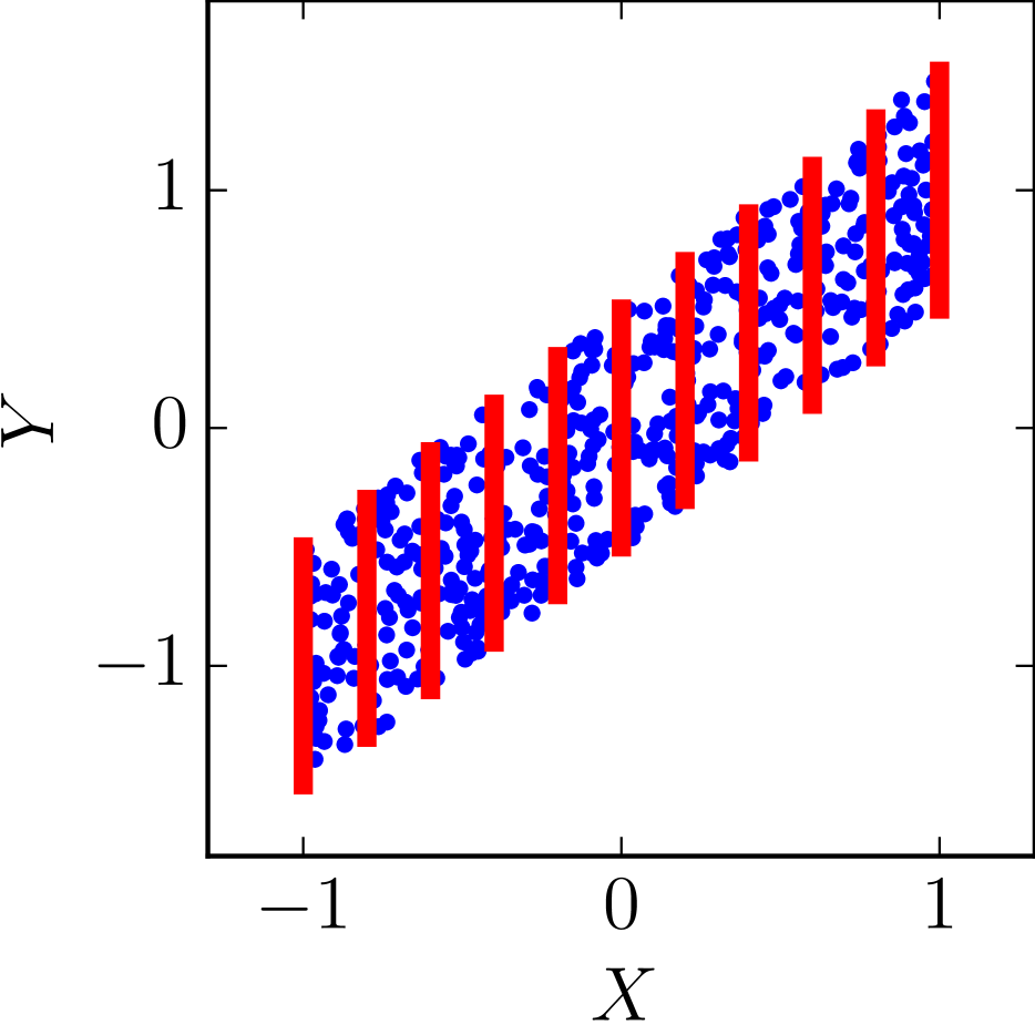
(a) $Y=F(X)+N$, $X\perp N$.

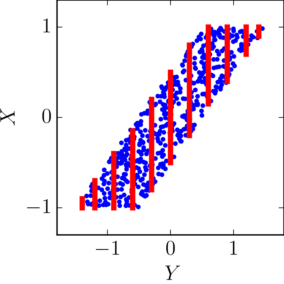
(b) $X=G(Y)+E$, $Y\not\perp E$.

Figure 1: Example of an Additive Noise Model (ANM).

In machine learning, these three types of statistical dependencies are exploited without distinction, as dependence is sufficient to perform optimal predictions about identically and independently distributed (iid) data (Schölkopf et al., 2012). However, we argue that taking into account the Principle of common cause would have far-reaching benefits in non-iid machine learning. For example, assume that we are interested in predicting the values of a target variable $Y$, given the values taken by two features $(X_{1},X_{2})$. Then, understanding the causal structure underlying $(X_{1},X_{2},Y)$ brings two benefits.

First, interpretability. Explanatory questions such as “Why does $Y=2$ when $(X_{1},X_{2})=(-1,3)$?”, and counterfactual questions such as “What value would have $Y$ taken, had $X_{2}=-3$?” cannot be answered using statistics alone, since their answers depend on the particular causal structure underlying the data.

Second, robustness. Predictors which estimate the values taken by a target variable $Y$ given only its direct causes are robust with respect to distributional shifts on their inputs. For example, let $X_{1}\sim{P}(X_{1})$, $Y\leftarrow F_{1}(X_{1})$, and $X_{2}\leftarrow F_{2}(X_{1})$. Then, the predictor ${\mathbb{E}}(Y{\,|\,}X_{1})$ is invariant to changes in the joint distribution $P(X_{1},X_{2})$ as long as the causal mechanism $F_{1}$ does not change. However, the predictor ${\mathbb{E}}(Y{\,|\,}X_{1},X_{2})$ can vary wildly even if the causal mechanism $F_{1}$ (the only one involved in computing $Y$) does not change (Peters et al., 2016; Rojas-Carulla et al., 2015).

The previous two points apply to the common “non-iid” situations where we have access to data drawn from some distribution ${P}$, but we are interested in some different but related distribution $\tilde{P}$. One natural way to phrase and leverage the similarities between $P$ and $\tilde{P}$ is in terms of shared causal structures (Peters, 2012; Lopez-Paz, 2016).

While it is indeed an attractive endeavor, discovering the causal relation between two random variables purely from observation is an impossible task when considered in full generality. Indeed, any of the three causal structures outlined in Principle 1 could explain the observed dependency between two random variables. However, one can in many cases impose assumptions to render the causal relation between two variables identifiable from their joint distribution. For example, consider the family of Additive Noise Models, or ANM (Hoyer et al., 2009; Peters et al., 2014; Mooij et al., 2016). In ANM, one assumes that the causal model has the form $Y=F(X)+N$, where $X\perp N$. It turns out that, under some assumptions, the reverse ANM $X=G(Y)+E$ will not satisfy the independence assumption $Y\perp E$ (Fig. 1). The statistical dependence shared by the cause and noise in the wrong causal direction is the footprint that renders the causal relation between $X$ and $Y$ identifiable from statistics alone.

In situations where the ANM assumption is not satisfied (e.g., multiplicative or heteroskedastic noise) one may prefer learning-based causal discovery tools, such as the Randomized Causation Coefficient (Lopez-Paz et al., 2015). RCC assumes access to a causal dataset $D=\{(S_{i},l_{i})\}_{i=1}^{n}$, where $S_{i}=(x_{i,j},y_{i,j})_{j=1}^{n_{i}}\sim P^{i}(X_{i},Y_{i})$ is a bag of examples drawn from some distribution $P^{i}$, $\ell_{i}=+1$ if $X_{i}\to Y_{i}$, and $\ell_{i}=-1$ if $X_{i}\leftarrow Y_{i}$. By featurizing each of the training distribution samples $S_{i}$ using kernel mean embeddings (Smola et al., 2007), RCC learns a binary classifier on $D$ to reveal the causal footprints necessary to classify new pairs of random variables.

However, both ANM and RCC based methods need $n\gg 1$ samples from $P(X,Y)$ to classify the causal relation between the random variables $X$ and $Y$. Therefore, these methods are not suited to infer the causal relation between static entities such as, for instance, one painting and its fraudulent copy. In the following section, we propose a framework to extend the state-of-the-art in causal discovery methods to this important case.

3 The Main Concepts: Static Entities, Proxy Variables and Proxy Projections

In the following, we consider two static entities $x,y$ in some space $\mathcal{S}$ that satisfy the relation “$x$ causes $y$”. Formally, this causal relation manifests the existence of a (possibly noisy) mechanism $f$ such that the value $y$ is computed as $y\leftarrow f(x)$. This asymmetric assignment guarantees changes in the static cause $x$ would lead to changes in the static effect $y$, but the converse would not hold.

As mentioned previously, traditional causal discovery methods cannot be directly applied to static entities. In order to discover the causal relation between the pair of static entities $x$ and $y$, we introduce two main concepts: proxy variables $W$, and proxy projections $\pi$.

First, a proxy random variable $W$ is a random variable taking values in some set $\mathcal{W}$, which can be understood as a random source of information related to $x$ and $y$. This definition is on purpose rather vague and will be illustrated through several examples in the following sections.

Second, a proxy projection is a function $\pi:\mathcal{W}\times\mathcal{S}\to\mathbb{R}$. Using a proxy variable and projection, we can construct a pair of scalar random variables $A=\pi(W,x)$ and $B=\pi(W,y)$. A proxy variable and projection are causal if the pair of random entities $(A,B)$ share the same causal footprint as the pair of static entities $(x,y)$.

If the proxy variable and projection are causal, we may estimate the cause-effect relation between the static entities $x$ and $y$ in three steps. First, draw $(a_{1},b_{1}),\ldots,(a_{n},b_{n})$ from $P(A,B)$. Second, use an observational causal discovery algorithm to estimate the cause-effect relation between $A$ and $B$ given $\{(a_{i},b_{i})\}_{i=1}^{n}$. Third, conclude “$x$ causes $y$” if $A\to B$, or “$y$ causes $x$” if $A\leftarrow B$. This process is summarized in Figure 2.

Note that the causal relation $X\to Y$ does not imply the causal relation $A\to B$ in the interventional sense: even if $A$ is a copy of $X$ and $B$ is a copy of $Y$, intervening on $A$ will not change $B$! We only care here about the presence of statistically observable causal footprints between the variables. Furthermore, our framework extends readily to the case where $x$ and $y$ live in different modalities (say, $x$ is an image and $y$ is a piece of audio describing the image). In this case, all we need is a proxy variable $W=(W_{x},W_{y})$ and a pair of proxy projections $(\pi_{x},\pi_{y})$ with the appropriate structure. For simplicity and throughout this paper, we will choose our proxy variables and projections based on domain knowledge. Learning proxy variables and projections from data is an exciting area left for future research.

Figure 2: A pair of static entities $(x,y)$ share a causal relation of interest (thick blue arrow). A proxy variable $W$, together with a proxy projection $\pi$ produces the random entities $(A,B)$, that share the causal footprint of $(x,y)$, denoted by the dotted blue arrow.

4 Causal Discovery Using Proxies in Images

Consider the two images shown in Figure 3. The image on the left is an unprocessed photograph of the Tübingen Neckarfront, while the one on the right is the same photograph after being stylized with the algorithm of Gatys et al. (2016). From a causal point of view, the unprocessed image $x$ is the cause of the stylized image $y$. How can we leverage the ideas from Section 3 to recover such causal relation?

The following is one possible solution. Assume that the two images are represented by pixel intensity vectors $x$ and $y$, respectively. For $n\gg 1$ and $j=1,\ldots,n$:

• Draw a mask-image $w_{j}$, which contains ones inside a patch at random coordinates, and zeroes elsewhere.

• Compute $a_{j}=\langle w_{j},x\rangle$, and $b_{j}=\langle w_{j},y\rangle$.

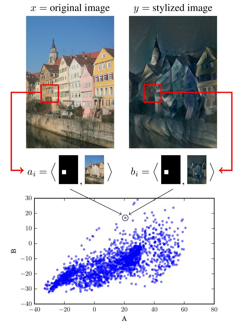
Figure 3: Sampling random patches at paired locations produces a proxy variable to discover the causal relation between two images.

This process returns a sample $\{(a_{j},b_{j})\}_{j=1}^{n}$ drawn from $P(A,B)$, the joint distribution of the two scalar random variables $(A,B)$. The conversion from static entities $(x,y)$ to random variables $(A,B)$ is obtained by virtue of i) the randomness generated by the proxy variable $W$, which in this particular case is incarnated as random masks and ii) a causal projection $\pi$, here a simple dot product.

At this point, if the causal footprint between the random entities $(A,B)$ resembles the causal footprint between $x$ and $y$, we can apply a regular causal discovery algorithm to $(A,B)$ to estimate the causal relation between $x$ and $y$.

4.1 Towards a Theoretical Understanding

The intuition behind causal discovery using proxy variables is that, although we observe $(x,y)$ as static entities, these are underlyingly complex, high-dimensional, structured objects that carry rich information about their causal relation. The proxy variable $W$ introduces randomness to sample different views of the high-dimensional causal structures, and $\pi$ summarizes those views into scalar values. But why should the causal footprint of these summaries cue the causal relation between $x$ and $y$?

We formalize this question for the specific case of stylized images, where $x$ is the original image and $y$ its stylized version. Let the causal mechanism mapping $x$ to $y$ operate locally. More precisely, assume that each $k$-subset $y_{S_{i}}$ in the stylized image is computed from the $k$-subset $x_{S_{i}}$ in the original image, as described by the ANM:

$$y_{S_{i}}=f(x_{S_{i}})+\epsilon_{S_{i}}.$$

Then, the stylized image $y=F(x)+\epsilon$, where $F(x)_{S_{i}}=f(x_{S_{i}})$. For simplicity, assume that $f(x_{S})=g(\beta x_{S})$ where $\beta$ is a $k\times k$ matrix and $g$ acts element-wise. Then, let $P(W)$ be a distribution over masks extracting random $k$-subsets, and let $\pi(\cdot,\cdot)=\langle\cdot,\cdot\rangle$, to obtain:

$$A=\pi(W,x) =\langle W,x\rangle,$$

$$B=\pi(W,y) =\langle W,y\rangle$$

$$=\sum_{j=1}^{k}g_{j}\left(\sum_{l=1}^{k}\beta_{jl}(x_{S})_{l}\right)+N$$

$$=\sum_{j=1}^{k}g_{j}\left(\sum_{l=1}^{k}\alpha_{j}A\right)+N$$

where $N=\sum_{j=1}^{k}(\epsilon_{S})_{j}$, and where we assume that $\beta$ is such that $\alpha_{j}=\beta_{jl}$ for all $j\leq k$. Since $A\perp N$, the pair $(A,B)$ also follows an ANM. We leave for future work the investigation on identifiability conditions for causal inference using proxy variables.

4.2 Numerical Simulations

In order to illustrate the use of causal discovery using proxy variables in images, we conducted two small experiments. In these experiments, we extract $n=1024$ square patches of size $k=10$ pixels, and use the Additive Noise Model (Hoyer et al., 2009) to estimate the causal relation between the constructed scalar random variables $A$ and $B$.

First, we collected $14$ unprocessed images together with $34$ stylizations (including the one from Figure 3), made using the algorithm of Gatys et al. (2016). When applying causal discovery using proxy variables to this dataset, we can correctly identify the correct direction of causation from the original image to its stylized version in $80\%{}$ of the cases.

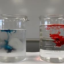
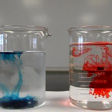
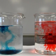
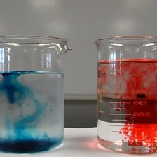
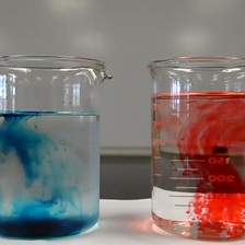
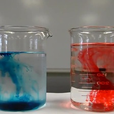
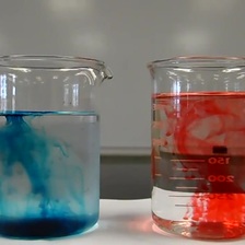
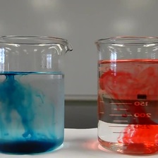
Figure 4: Causal discovery using proxy variables uncovers the causal time signal to reorder a shuffled sequence of video frames.

Second, we decomposed a video of drops of ink mixing with water into $8$ frames $\{(x_{i})\}_{i=1}^{8}$, shown in Figure 4. Using the same mask proxy variable as above, we construct an $8\times 8$ matrix $M$ such that $M_{ij}=1$ if $x_{i}\rightarrow x_{j}$ according to our method and $M_{ij}=0$ otherwise. Then, we consider $M$ to be the adjacency matrix of the causal DAG describing the causal structure between the $8$ frames. By employing topological sort on this graph, we were able to obtain the true ordering, unique among the $40,320$ possible orderings.

5 Causal Discovery Using Proxies in NLP

As our main case study, consider discovering the causal relation between pairs of words appearing in a large corpus of natural language. For instance, given the pair of words (virus, death), which represent our static entities $x$ and $y$, together with a large corpus of natural language, we want to recover causal relations such as “virus $\to$ death”, “sun $\to$ radiation”, “trial $\to$ sentence”, or “drugs $\to$ addiction”.

This problem is extremely challenging for two reasons. First, word pairs are extremely varied in nature (compare “avocado causes guacamole” to “cat causes purr”), and some are very rare (“wrestler causes pin”). Second, the causal relation between two words can always be tweaked in context-specific ways. For instance, one can construct sentences where “virus causes death” (e.g., the virus led to a quick death), but also sentences where “death causes virus” (e.g., the multiple deaths in the area further spread the virus). We are hereby interested in the canonical causal relation between pairs of words, assumed by human subjects when specific contexts are not provided (see Section 5.2). Furthermore, our interest lies in discovering the causal relation between pairs of words without the use of language-specific knowledge or heuristics. To the contrary, we aim to discover such causal relations by using generic observational causal discovery methods, such as the ones described in Section 2.

In the following, Section 5.1 frames this problem in the language of causal discovery between static entities. Then, Section 5.2 introduces a novel, human-generated, human-validated dataset to test our methods. Section 5.3 reviews prior work on causal discovery in language. Finally, Section 5.4 presents experiments evaluating our methods.

5.1 Static Entities, Proxies, and Projections for NLP

In the language of causal discovery with proxies, a pair of words is a pair of static entities: $(x,y)=(\text{virus},\text{death})$. In order to discover the causal relation between $x$ and $y$, we are in need of a proxy variable $W$, as introduced in Section 3. We will use a simple proxy: let $P(W=w)$ be the probability of the word $w$ appearing in a sentence drawn at random from a large corpus of natural language.

Using the proxy $W$, we need to define the pair of random variables $A=\pi(W,x)$ and $B=\pi(W,y)$ in terms of a causal projection $\pi$. Once we have defined the causal projection $\pi$, we can sample $w_{1},\ldots,w_{n}\sim P(W)$, construct $a_{i}=\pi(w_{i},x)$, $b_{i}=\pi(w_{i},y)$, and apply a causal discovery algorithm to the sample $\{(a_{i},b_{i})\}_{i=1}^{n}$. Specifically, we estimate $P(W)$ from a large corpus of natural language, and sample $n=10,000$ words without replacement.

Throughout our experimental evaluation, we will use and compare different proxy projections $\pi(w,x)$:

• $\pi_{\text{w2vii}}(w,x)=\langle v^{i}_{w},v^{i}_{x}\rangle$, where $v^{i}_{z}\in\mathbb{R}^{d}$ is the input word2vec representation (Mikolov et al., 2013) of the word $z$. The dot-product $\langle v^{i}_{w},v^{i}_{x}\rangle$ measures the similarity in meaning between the pair of words $(w,x)$.

• $\pi_{\text{w2vio}}(w,x)=\langle v^{i}_{w},v^{o}_{x}\rangle$, where $v^{o}_{z}\in\mathbb{R}^{d}$ is the output word2vec representation of the word $z$. The dot-product $\langle v^{i}_{w},v^{o}_{x}\rangle$ is an unnormalized estimate of the conditional probability $p(x|w)$ (Melamud et al., 2015).

• $\pi_{\text{w2voi}}(w,x)=\langle v^{o}_{w},v^{i}_{x}\rangle$, an unnormalized estimate of the conditional probability $p(w|x)$.

• $\pi_{\text{counts}}(w,x)=p(w,x)$, where the pmf $p(w,x)$ is directly estimated from counting within-sentence co-occurrences in the corpus.

• $\pi_{\text{prec-counts}}(w,x)$ similar to the one above, but computed only over sentences where $w$ precedes $x$.

• $\pi_{\text{pmi}}(w,x)=p(w,x)/(p(w)p(x))$, where the pmfs $p(w)$, $p(x)$, and $p(w,x)$ are estimated from counting words and (sentence-based) co-occurrences in the corpus. The log of this quantity is known as point-wise mutual information, or PMI (Church & Hanks, 1990).

• $\pi_{\text{prec-pmi}}(w,x)$, similar to the one above, but computed only over sentences where $w$ precedes $x$.

Applying the causal projections to our sample from proxy $W$, we construct the $n$-vector

$$\Pi_{\text{proj}}^{x} =(\pi_{\text{proj}}(w_{1},x),\ldots,\pi_{\text{proj}}(w_{n},x)),$$ (1)

and similarly for $\Pi_{\text{proj}}^{y}$, where

$$\text{proj}\in\{ \text{w2vii},\text{w2vio},\text{w2voi},$$

$$\text{counts},\text{prec-counts},\text{pmi},\text{prec-pmi}\}.$$ (2)

In particular, we use the skip-gram model implementation of fastText (Bojanowski et al., 2016) to compute $300-$dimensional word2vec representations.

5.2 A Real-World Dataset of Cause-Effect Words

We introduce a human-elicited, human-filtered dataset of $10,000$ pairs of words with a known causal relation. This dataset was constructed in two steps:

• We asked workers from Amazon Mechanical Turk to create pairs of words linked by a causal relation. We provided the turks with examples of words with a clear causal link (such as “sun causes radiation”) and examples of related words not sharing a causal relation (such as “knife” and “fork”). For details, see Appendix A.

• Each of the pairs collected from the previous step was randomly shuffled and submitted to $20$ different turks, none of whom had created any of the word pairs. Each turk was required to classify the pair of words $(x,y)$ as “$x$ causes $y$”, “$y$ causes $x$”, or “$x$ and $y$ do not share a causal relation”. For more details, see Appendix B.

This procedure resulted in a dataset of $10,000$ causal word pairs $(x,y)$, each accompanied with three numbers: the number of turks that voted “$x$ causes $y$”, the number of turks that voted “$y$ causes $x$”, and the number of turks that voted “$x$ and $y$ do not share a causal relation”.

5.3 Causal Relation Discovery in NLP

The NLP community has devoted much attention to the problem of identifying the semantic relation holding between two words, with causality as a special case. Girju et al. (2009) discuss the results of the large shared task on relation classification they organized (their benchmark included only 220 examples of cause-effect). The task required recognizing relations in context, but, as discussed by the authors, most contexts display the default relation we are after here (e.g., “The mutant virus gave him a severe flu” instantiates the default relation in which virus is the cause, flu is the effect). All participating systems used extra resources, such as ontologies and syntactic parsing, on top of corpus data. They are thus outside the scope of the purely corpus-based methods we are considering here.

Most NLP work specifically focusing on the causality relation relies on informative linking patterns co-occurring with the target pairs (such as, most obviously, the conjunction because). These patterns are extracted and processed with sophisticated methods, involving annotation, ontologies, bootstrapping and/or manual filtering (see, e.g., Blanco et al. 2008 Hashimoto et al. 2012, Radinsky et al. 2012, and references therein). We experimented with extracting linking patterns from our corpus, but, due to the relatively small size of the latter, results were extremely sparse (note that patterns can only be extracted from sentences in which both cause and effect words occur). More recent work started looking at causal chains of events as expressed in text (see Mirza & Tonelli 2016 and references therein). Applying our generic method to this task is a direction for future work.

A semantic relation that received particular attention in NLP is that of entailment between words (dog entails animal). As causality is intuitively related to entailment, we will apply below entailment detection methods to cause/effect classification. Most lexical entailment methods rely on distributional representations of the words in the target pair. Traditionally, entailing pairs have been identified with unsupervised asymmetric similarity measures applied to distributed word representations (Geffet & Dagan, 2005; Kotlerman et al., 2010; Lenci & Benotto, 2012; Weeds et al., 2004). We will test one of these related measures, namely, Weeds Precision (WS). More recently, Santus et al. 2014 showed that the relative entropy of distributed vectors representing the words in a pair is an effective cue to which word is entailing the other, and we also look at entropy for our task. However, the most effective method to detect entailment is to apply a supervised classifier to the concatenation of the vectors representing the words in a pair (Baroni et al., 2012; Roller et al., 2014; Weeds et al., 2014).

5.4 Experiments

We evaluate a variety of methods to discover the causal relation between two words appearing in a large corpus of natural language. We study methods that fall within three categories: baselines, distribution-based causal discovery methods, and feature-based supervised methods. These three families of methods consider an increasing amount of information about the task at hand, and therefore exhibit an increasing performance up to $85\%{}$ classification accuracy.

All our computations will be based on the full English Wikipedia, as post-processed by Matt Mahoney (see http://www.mattmahoney.net/dc/textdata.html). We study the $N=1,970$ pairs of words out of $10,000$ from the dataset described in Section 5.2 that achieved a consensus across at least $18$ out of $20$ turks. We use RCC to estimate the causal relation between pairs of random variables.

5.4.1 Baselines

These are a variety of unsupervised, heuristic baselines. Each baseline computes two scores, denoted by $S_{x\to y}$ and $S_{x\leftarrow y}$, predicting $x\to y$ if $\text{$S_{x\to y}${}}>\text{$S_{x\leftarrow y}${}}$, and $x\leftarrow y$ if $\text{$S_{x\to y}${}}<\text{$S_{x\leftarrow y}${}}$. The baselines are:

• frequency: $S_{x\to y}$ is the number of sentences where $x$ appears in the corpus, and $S_{x\leftarrow y}$ is the number of sentences where $y$ appears in the corpus.

• precedence: considering only sentences from the corpus where both $x$ and $y$ appear, $S_{x\to y}$ is the number of sentences where $x$ occurs before $y$, and $S_{x\leftarrow y}$is the number of sentences where $y$ occurs before $x$.

• counts (entropy): $S_{x\to y}$ is the entropy of $\Pi_{\text{counts}}^{x}$, and $S_{x\leftarrow y}$ is the entropy of $\Pi_{\text{counts}}^{y}$, as defined in (1).

• counts (WS): Using the WS measure of Weeds & Weir (2003), $\text{$S_{x\to y}${}}=\text{WS}(\Pi_{\text{counts}}^{x},\Pi_{\text{counts}}^{y})$, and $\text{$S_{x\leftarrow y}${}}=\text{WS}(\Pi_{\text{counts}}^{y},\Pi_{\text{counts}}^{x})$.

• prec-counts (entropy): $S_{x\to y}$ is the entropy of $\Pi_{\text{prec-counts}}^{x}$, and $S_{x\leftarrow y}$ is the entropy of $\Pi_{\text{prec-counts}}^{y}$ (1).

• prec-counts (WS): analogous to the previous.

The baselines PMI (entropy), PMI (WS), prec-PMI (entropy), prec-PMI (WS) are analogous to the last four, but use $(\Pi_{\text{(prec-)pmi}}^{x},\Pi_{\text{(prec-)pmi}}^{y})$ instead of $(\Pi_{\text{(prec-)counts}}^{x},\Pi_{\text{(prec-)counts}}^{y})$. Figure 5 shows the performance of these baselines in blue.

5.4.2 Distribution-based causal discovery methods

These methods implement our framework of causal discovery using proxy variables. They classify $n$ samples from a 2-dimensional probability distribution as a whole. Recall that a vocabulary $(w_{j})_{j=1}^{n}$ drawn from the proxy is available. Given $N$ word pairs $(x_{i},y_{i})$, this family of methods constructs a dataset $D=\left\{(\{(a_{j}^{i},b_{j}^{i})\}_{j=1}^{n},\ell^{i})\right\}_{i=1}^{N}$, where $a_{j}^{i}=\pi_{\text{proj}}({w}_{j},x_{i})$, $b_{j}^{i}=\pi_{\text{proj}}({w}_{j},y_{i})$, $\ell^{i}=+1$ if $x_{i}\to y_{i}$ and $\ell^{i}=-1$ otherwise. In short, $D$ is a dataset of $N$ “scatterplots” annotated with binary labels. The $i$-th scatterplot contains $n$ 2-dimensional points, which are obtained by applying the causal projection to both $x_{i}$ and $y_{i}$, against the $n$ vocabulary words drawn from the proxy.

The samples $(a_{j}^{i},b_{j}^{i})_{j=1}^{n}$ are computed using a deterministic projection of iid draws from the proxy, meaning that $\{(a_{j}^{i},b_{j}^{i})\}_{j=1}^{n}\sim P^{n}(A^{i},B^{i})$. Therefore, we could permute the points inside each scatterplot without altering the results of these methods. In principle, we could also remove some of the points in the scatterplot without a significant drop in performance. Therefore, these methods search for causal footprints at the 2-dimensional distribution level, and we term them distribution-based causal discovery methods.

The methods in this family first split the dataset $D$ into a training set $D_{\text{tr}}$ and a test set $D_{\text{te}}$. Then, the methods train RCC on the training set $D_{\text{tr}}$, and test its classification accuracy on $D_{\text{te}}$. This process is repeated ten times, splitting at random $D$ into a training set containing $75\%{}$ of the pairs, and a test set containing $25\%{}$ of the pairs. Each method builds on top of a causal projection from (2) above. Figure 5 shows the test accuracy of these methods in green.

5.4.3 Feature-based supervised methods

These methods use the same data generated by our causal projections, but treat them as fixed-size vectors fed to a generic classifier, rather than random samples to be analyzed with an observational causal discovery method. They can be seen as an oracle to upper-bound the amount of causal signals (and signals correlated to causality) contained in our data. Specifically, they use $2n$-dimensional vectors given by the concatenation of those in (1). Given $N$ word pairs $(x_{i},y_{i})$, they build a dataset $D=\left((\Pi_{\text{proj}}^{x_{i}},\Pi_{\text{proj}}^{y_{i}}),\ell^{i}\right)_{i=1}^{N}$, where $\ell^{i}=+1$ if $x_{i}\to y_{i}$, $\ell^{i}=-1$ if $x_{i}\leftarrow y_{i}$, and “proj” is a projection from (2). Next, we split the dataset $D$ into a training set $D_{\text{tr}}$ containing $75\%{}$ of the pairs, and a disjoint test set $D_{\text{te}}$ containing $25\%{}$ of the pairs. To evaluate the accuracy of each method in this family, we train a random forest of $500$ trees using $D_{\text{tr}}$, and report its classification accuracy over $D_{\text{te}}$. This process is repeated ten times, by splitting the dataset $D$ at random. The results are presented as red bars in Figure 5. We also report the classification accuracy of training the random forest on the raw word2vec representations of the pair of words (top three bars).

5.4.4 Discussion of results

Baseline methods are the lowest performing, up to $59\%{}$ test accuracy. We believe that the performance of the best baseline, precedence, is due to the fact that most Wikipedia is written in the active voice, which often aligns with the temporal sequence of events, and thus correlates with causality.

The feature-based methods perform best, achieving up to $85\%{}$ test classification accuracy. However, feature-based methods enjoy the flexibility of considering each of the $n=10,000$ elements in the causal projection as a distinct feature. Therefore, feature-based methods do not focus on patterns to be found at a distributional level (such as causality), and are vulnerable to permutation or removal of features. We believe that feature-based methods may achieve their superior performance by overfitting to biases in our dataset, which are not necessarily related to causality.

Impressively, the best distribution-based causal discovery method achieves $75\%{}$ test classification accuracy, which is a significant improvement over the best baseline method. Importantly, our distribution-based methods take a whole $2$-dimensional distribution as input to the classifier; as such, these methods are robust with respect to permutations and removals of the $n$ distribution samples. We find it encouraging that the best distribution-based method is the one based on $\pi_{\text{w2voi}}$. This suggests the intuitive interpretation that the distribution of a vocabulary conditioned on the cause word causes the distribution of the vocabulary conditioned on the effect word. Even more encouragingly, Figure 6 shows a positive dependence between the test classification accuracy of RCC and the confidence of human annotations, when considering the test classification accuracy of all the causal pairs annotated with a human confidence of at least $\{0,20,40,50,60,70,80,90\}$. Thus, our proxy variables and projections arguably capture a notion of causality aligned with the one of human annotators.

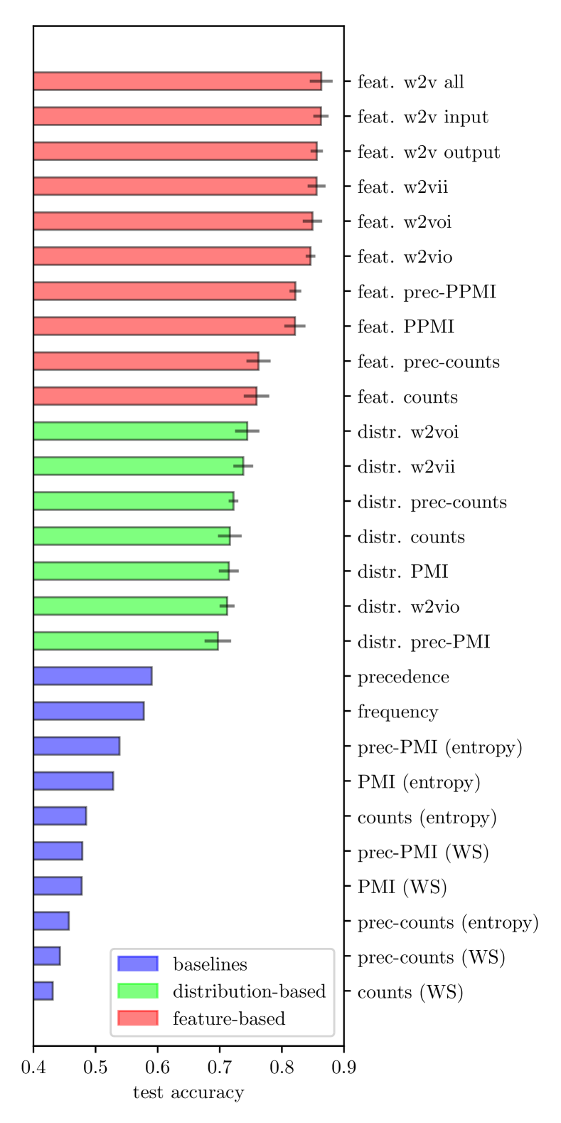
Figure 5: Results for all methods on the NLP experiment. Accuracies above $52\%{}$ are statistically significant with respect to a Binomial test at a significance level $\alpha=0.05$.

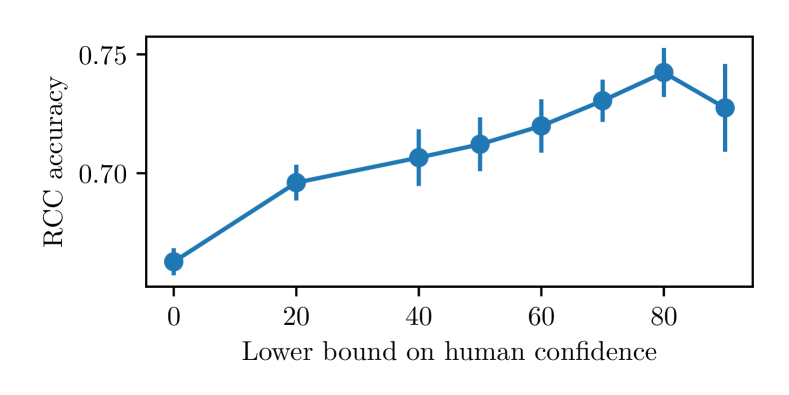
Figure 6: RCC accuracy versus human confidence.

6 Proxy Variables in Machine Learning

The central concept in this paper is the one of proxy variable. This is a variable $W$ providing a random source of information related to $x$ and $y$.

However, we can consider the reverse process of using a static entity $w$ to augment random statistics about a pair of random variables $X$ and $Y$. As it turns out, this could be an useful process in general prediction problems.

To illustrate, consider a supervised learning problem mapping a feature random variable $X$ into a target random variable $Y$. Such problem is often solved by considering a sample $\{(x_{i},y_{i})\}_{i=1}^{n}\sim P^{n}(X,Y)$. In this scenario, we may contemplate an unpaired, external, static source of information $w$ (such as a memory), which might help solving the supervised learning problem at hand. One could incorporate the information in the static source $w$ by constructing the proxy projection $w_{i}=\pi(x_{i},w)$, and add them to the dataset to obtain $\{((x_{i},w_{i}),y_{i})\}_{i=1}^{n}$ to build the predictor $f(x,\pi(x,w))$.

7 Conclusion

We have introduced the necessary machinery to estimate the causal relation between pairs of static entities $x$ and $y$ — one piece of art and its forgery, one document and its translation, or the concepts underlying a pair of words appearing in a corpus of natural language. We have done so by introducing the tool of proxy variables and projections, reducing our problem to one of observational causal inference between random entities. Throughout a variety of experiments, we have shown the empirical effectiveness of our proposed method, and we have connected it to the general problem of incorporating external sources of knowledge as additional features in machine learning problems.

 

Supplementary material to Causal discovery using proxy variables

 

Appendix A Instructions for word pair creators

We will ask you to write word pairs (for instance, WordA and WordB) for which you believe the statement “WordA causes WordB” is true.

To provide us with high quality word pairs, we ask you to follow these indications:

• All word pairs must have the form “WordA $\rightarrow$ WordB”. It is essential that the first word (WordA) is the cause, and the second word (WordB) is the effect.

• WordA and WordB must be one word each (no spaces, and no “recessive gene $\rightarrow$ red hair”). Avoid compound words such as “snow-blind”.

• In most situations, you may come up with a word pair that can be justified both as “WordA $\rightarrow$ WordB” and “WordB $\rightarrow$ WordA”. In such situations, prefer the causal direction with the easiest explanation. For example, consider the word pair “virus $\rightarrow$ death”. Most people would agree that “virus causes death“. However, “death causes virus” can be true in some specific scenario (for example, “because of all the deaths in the region, a new family of virus emerged.”). However, the explanation “virus causes death“ is preferred, because it is more general and depends less on the context.

• We do not accept word pairs with an ambiguous causal relation, such as “book - paper”.

• We do not accept simple variations of word pairs. For example, if you wrote down “dog $\rightarrow$ bark”, we will not credit you for other pairs such as “dogs $\rightarrow$ bark” or “dog $\rightarrow$ barking”.

• Use frequent words (avoid strange words such as “clithridiate”).

• Do not rely on our examples, and use your creativity. We are grateful if you come up with diverse word pairs! Please do not add any numbers (for example, “1 - dog $\rightarrow$ bark”). For your guidance, we provide you examples of word pairs that belong to different categories. Please bear in mind that we will reward your creativity: therefore, focus on providing new word pairs with an evident causal direction, and do not limit yourself to the categories shown below.

1) Physical phenomenon: there exists a clear physical mechanism that explains why “WordA $\rightarrow$ WordB”.

• sun $\rightarrow$ radiation (The sun is a source of radiation. If the sun were not present, then there would be no radiation.)

• altitude $\rightarrow$ temperature

• winter $\rightarrow$ cold

• oil $\rightarrow$ energy

2) Events and consequences: WordA is an action or event, and WordB is a consequence of that action or event.

• crime $\rightarrow$ punishment

• accident $\rightarrow$ death

• smoking $\rightarrow$ cancer

• suicide $\rightarrow$ death

• call $\rightarrow$ ring

3) Creator and producer: WordA is a creator or producer, WordB is the creation of the producer.

• writer $\rightarrow$ book (the creator is a person)

• painter $\rightarrow$ painting

• father $\rightarrow$ son

• dog $\rightarrow$ bark

• bacteria $\rightarrow$ sickness

• pen $\rightarrow$ drawing (the creator is an object)

• chef $\rightarrow$ food

• instrument $\rightarrow$ music

• bomb $\rightarrow$ destruction

• virus $\rightarrow$ death

4) Other categories! Up to you, please use your creativity!

• fear $\rightarrow$ scream

• age $\rightarrow$ salary

Appendix B Instructions for word pair validators

Please classify the relation between pairs of words A and B into one of three categories: either “A causes B”, “B causes A”, or “Non-causal or unrelated”.

For example, given the pair of words “virus and death”, the correct answer would be:

• virus causes death (correct);

• death causes virus (wrong);

• non-causal or unrelated (wrong).

Some of the pairs that will be presented are non-causal. This may happen if:

• The words are unrelated, like “toilet and beach”.

• The words are related, but there is no clear causal direction. This is the case of “salad and lettuce”, since we can eat salad without lettuce, or eat lettuce in a burger.

To provide us with high quality categorization of word pairs, we ask you to follow these indications:

• Prefer the causal direction with the simplest explanation. Most people would agree that “virus causes death”. However, “death causes virus” can be true in some specific scenario (for example, “because of all the deaths in the region, a new virus emerged.”). However, the explanation “virus causes death” is preferred, because it is true in more general contexts.

• If no direction is clearer, mark the pair as non-causal. Here, conservative is good!

• Think twice before deciding. We will present the pairs in random order!

Please classify all the presented pairs. If one or more has not been answered, the whole batch will be invalid. PLEASE DOUBLE CHECK THAT YOU HAVE ANSWERED ALL 40 WORD PAIRS.

Examples of causal word pairs:

• “sun and radiation”: sun causes radiation

• “energy and oil”: oil causes energy

• “punishment and crime”: crime causes punishment

• “instrument and music”: instrument causes music

• “age and salary”: age causes salary

Examples of non-causal word pairs:

• “video and games”: non-causal or unrelated

• “husband and wife”: non-causal or unrelated

• “salmon and shampoo”: non-causal or unrelated

• “knife and gun”: non-causal or unrelated

• “sport and soccer”: non-causal or unrelated

References

- Baayen (2001) Baayen, H. Word Frequency Distributions. Kluwer, 2001.
- Baroni et al. (2012) Baroni, M., Bernardi, R., Do, N.-Q., and Shan, C.-C. Entailment above the word level in distributional semantics. In EACL, 2012.
- Beebee et al. (2009) Beebee, H., Hitchcock, C., and Menzies, P. The Oxford handbook of causation. Oxford University Press, 2009.
- Blanco et al. (2008) Blanco, E., Castell, N., and Moldovan, D. Causal relation extraction. In LREC, 2008.
- Bojanowski et al. (2016) Bojanowski, P., Grave, E., Joulin, A., and Mikolov, T. Enriching word vectors with subword information. arXiv, 2016.
- Bottou (2014) Bottou, L. From machine learning to machine reasoning. Machine learning, 2014.
- Bottou et al. (2013) Bottou, L., Peters, J., Charles, D. X., Chickering, M., Portugaly, E., Ray, D., Simard, P. Y., and Snelson, E. Counterfactual reasoning and learning systems: the example of computational advertising. JMLR, 2013.
- Church & Hanks (1990) Church, K. and Hanks, P. Word association norms, mutual information, and lexicography. Computational linguistics, 1990.
- Cohen (2015) Cohen, P. R. DARPA’s Big Mechanism program. Physical biology, 2015.
- Daniusis et al. (2012) Daniusis, P., Janzing, D., Mooij, J., Zscheischler, J., Steudel, B., Zhang, K., and Schölkopf, B. Inferring deterministic causal relations. arXiv, 2012.
- Gatys et al. (2016) Gatys, L. A., Ecker, A. S., and Bethge, M. Image style transfer using convolutional neural networks. In CVPR, 2016.
- Geffet & Dagan (2005) Geffet, M. and Dagan, I. The distributional inclusion hypotheses and lexical entailment. In ACL, 2005.
- Girju et al. (2009) Girju, R., Nakov, P., Nastase, V., Szpakowicz, S., Turney, P., and Yuret, D. Classification of semantic relations between nominals. Language Resources and Evaluation, 2009.
- Hashimoto et al. (2012) Hashimoto, C., Torisawa, K., De Saeger, S., Oh, J.-H., and Kazama, J. Excitatory or inhibitory: A new semantic orientation extracts contradiction and causality from the web. In EMNLP, 2012.
- Hoyer et al. (2009) Hoyer, P., Janzing, D., Mooij, J., Peters, J., and Schölkopf, B. Nonlinear causal discovery with additive noise models. In NIPS, 2009.
- Kotlerman et al. (2010) Kotlerman, L., Dagan, I., Szpektor, I., and Zhitomirsky-Geffet, M. Directional distributional similarity for lexical inference. Natural Language Engineering, 2010.
- Kuipers (1984) Kuipers, B. Commonsense reasoning about causality: deriving behavior from structure. Artificial intelligence, 1984.
- Lake et al. (2016) Lake, B. M., Ullman, T. D., Tenenbaum, J. B., and Gershman, S. J. Building machines that learn and think like people. arXiv, 2016.
- Lenci & Benotto (2012) Lenci, A. and Benotto, G. Identifying hypernyms in distributional semantic spaces. In *SEM, 2012.
- Levesque et al. (2012) Levesque, H., Davis, E., and Morgenstern, L. The Winograd Schema Challenge. In KR, 2012.
- Lopez-Paz (2016) Lopez-Paz, D. From dependence to causation. PhD thesis, University of Cambridge, 2016.
- Lopez-Paz et al. (2015) Lopez-Paz, D., Muandet, K., Schölkopf, B., and Tolstikhin, I. Towards a learning theory of cause-effect inference. In ICML, 2015.
- Melamud et al. (2015) Melamud, O., Levy, O., Dagan, I., and Ramat-Gan, I. A simple word embedding model for lexical substitution. In Workshop on Vector Space Modeling for Natural Language Processing, 2015.
- Mikolov et al. (2013) Mikolov, T., Chen, K., Corrado, G., and Dean, J. Efficient estimation of word representations in vector space. arXiv, 2013.
- Mirza & Tonelli (2016) Mirza, P. and Tonelli, S. CATENA: CAusal and TEmporal relation extraction from NAtural language texts. In COLING, 2016.
- Mooij et al. (2016) Mooij, J. M., Peters, J., Janzing, D., Zscheischler, J., and Schölkopf, B. Distinguishing cause from effect using observational data: methods and benchmarks. JMLR, 2016.
- Pearl (2009) Pearl, J. Causality: Models, Reasoning, and Inference. Cambridge University Press, 2nd edition, 2009.
- Peters (2012) Peters, J. Restricted structural equation models for causal inference. PhD thesis, ETH Zurich, 2012.
- Peters et al. (2014) Peters, J., Mooij, J., Janzing, D., and Schölkopf, B. Causal discovery with continuous additive noise models. JMLR, 2014.
- Peters et al. (2016) Peters, J., Bühlmann, P., and Meinshausen, N. Causal inference using invariant prediction: identification and confidence intervals. JRSS B, 2016.
- Radinsky et al. (2012) Radinsky, K., Davidovich, S., and Markovitch, S. Learning causality for news events prediction. In WWW, 2012.
- Reichenbach (1956) Reichenbach, H. The direction of time, 1956.
- Rojas-Carulla et al. (2015) Rojas-Carulla, M., Schölkopf, B., Turner, R., and Peters, J. Causal transfer in machine learning. arXiv, 2015.
- Roller et al. (2014) Roller, S., Erk, K., and Boleda, G. Inclusive yet selective: Supervised distributional hypernymy detection. In COLING, 2014.
- Santus et al. (2014) Santus, E., Lenci, A., Lu, Q., and Schulte im Walde, S. Chasing hypernyms in vector spaces with entropy. In EACL, 2014.
- Schölkopf et al. (2012) Schölkopf, B., Janzing, D., Peters, J., Sgouritsa, E., Zhang, K., and Mooij, J. On causal and anticausal learning. In ICML, 2012.
- Shimizu et al. (2006) Shimizu, S., Hoyer, P., Hyvärinen, A., and Kerminen, A. A linear non-gaussian acyclic model for causal discovery. JMLR, 2006.
- Smola et al. (2007) Smola, A., Gretton, A., Song, L., and Schölkopf, B. A Hilbert space embedding for distributions. In ALT. Springer, 2007.
- Waldrop (1987) Waldrop, M. M. Causality, structure, and common sense. Science, 1987.
- Weeds & Weir (2003) Weeds, J. and Weir, D. A general framework for distributional similarity. In EMNLP, 2003.
- Weeds et al. (2004) Weeds, J., Weir, D., and McCarthy, D. Characterising measures of lexical distributional similarity. In COLING, 2004.
- Weeds et al. (2014) Weeds, J., Clarke, D., Reffin, J., Weir, D., and Keller, B. Learning to distinguish hypernyms and co-hyponyms. In COLING, 2014.