How to Optimally Allocate Resources for Coded Distributed Computing?

Abstract

Today’s data centers have an abundance of computing resources, hosting server clusters consisting of as many as tens or hundreds of thousands of machines. To execute a complex computing task over a data center, it is natural to distribute computations across many nodes to take advantage of parallel processing. However, as we allocate more and more computing resources to a computation task and further distribute the computations, large amounts of (partially) computed data must be moved between consecutive stages of computation tasks among the nodes, hence the communication load can become the bottleneck. In this paper, we study the optimal allocation of computing resources in distributed computing, in order to minimize the total execution time in distributed computing accounting for both the duration of computation and communication phases. In particular, we consider a general MapReduce-type distributed computing framework, in which the computation is decomposed into three stages: Map, Shuffle, and Reduce. We focus on a recently proposed Coded Distributed Computing approach for MapReduce and study the optimal allocation of computing resources in this framework. For all values of problem parameters, we characterize the optimal number of servers that should be used for distributed processing, provide the optimal placements of the Map and Reduce tasks, and propose an optimal coded data shuffling scheme, in order to minimize the total execution time. To prove the optimality of the proposed scheme, we first derive a matching information-theoretic converse on the execution time, then we prove that among all possible resource allocation schemes that achieve the minimum execution time, our proposed scheme uses the exactly minimum possible number of servers.

I Introduction

In recent years, distributed systems like Apache Spark [1] and computational primitives like MapReduce [2], Dryad [3], and CIEL [4] have gained significant traction, as they enable the execution of production-scale computation tasks on data sizes of the order of tens of terabytes and more. The design of these modern distributed computing platforms is driven by scaling out computations across clusters consisting of as many as tens or hundreds of thousands of machines. As a result, there is an abundance of computing resources that can be utilized for distributed processing of computation tasks. However, as we allocate more and more computing resources to a computation task and further distribute the computations, a large amount of (partially) computed data must be moved between consecutive stages of computation tasks among the nodes, hence the communication load can become the bottleneck. This gives rise to an important problem:

• How should we optimally allocate computing resources for distributed processing of a computation task in order to minimize its total execution time (accounting for both the duration of computation and communication phases)?

This problem has indeed attracted a lot of attention in recent years, and it has been broadly studied in various settings (see, e.g., [5, 6, 7, 8, 9]). In this paper, we study resource allocation problem in the context of a recently proposed coding framework for distributed computing, namely Coded Distributed Computing [10], which allows to optimally trade computation load with communication load in distributed computing. The key advantage of this framework is that it quantitatively captures the relation between computation time and communication time in distributed computing, which is crucial for resource allocation problems.

More formally, we consider a general MapReduce-type framework for distributed computing (see, e.g., [2, 1]), in which the overall computation is decomposed to three stages, Map, Shuffle, and Reduce that are executed distributedly across several computing nodes. In the Map phase, each input file is processed locally, in one (or more) of the nodes, to generate intermediate values. In the Shuffle phase, for every output function to be calculated, all intermediate values corresponding to that function are transferred to one of the nodes for reduction. Finally, in the Reduce phase all intermediate values of a function are reduced to the final result.

In Coded Distributed Computing, we allow redundant execution of Map tasks at the nodes, since it can result in significant reductions in data shuffling load by enabling in-network coding. In fact, in [11, 10] it has been shown that by assigning the computation of each Map task at $r$ carefully chosen nodes, we can enable novel coding opportunities that reduce the communication load by exactly a multiplicative factor of the computation load $r$. For example, the communication load can be reduced by more than 50% when each Map task is computed at only one other node (i.e., $r=2$).

Based on this framework, we consider two types of implementations: 1) Sequential Implementation. The above three phases take place one after another sequentially. In this case, the overall execution time $T_{\textup{sequential}}=T_{\textup{map}}+T_{\textup{shuffle}}+T_{\textup{reduce}}$. 2) Parallel Implementation. The Shuffle phase happens in parallel with the Map phase. In this case, the overall execution time becomes $T_{\textup{parallel}}=\max\{T_{\textup{map}},T_{\textup{shuffle}}\}+T_{\textup{reduce}}$. Then the considered resource allocation problem for e.g., the sequential implementation can (informally) be formulated as the following optimization problem.

In this paper, we exactly solve the above optimization problem and its counterpart for the parallel implementation. In particular, for each implementation, we propose an optimal resource allocation scheme that exactly achieves the minimum execution time. In the proposed scheme to compute $Q$ output functions, for some design parameter $r^{*}$, we use a number of $Q+\lceil\frac{Q}{r^{*}}\rceil$ server nodes for computation. These servers are split into two groups that are termed as the “solvers” and the “helpers”. There are $Q$ solver nodes, each computing a distinct Reduce function. The remaining $\lceil\frac{Q}{r^{*}}\rceil$ nodes are helpers, on which Map functions are computed to facilitate a more efficient data shuffling process. No Reduce function is computed on helpers themselves. In the Map phase, each input file is repetitively mapped on $r^{*}$ solver nodes according to a specified pattern. On the other hand, on the helper nodes, all input files are evenly partitioned and assigned for mapping, without any repetition. Then in the Shuffle phase, the communication is solely from the helpers to the solvers. In particular, based on the locally computed intermediate values in the Map phase, each helper node constructs coded multicast messages that are simultaneously delivering required intermediate values to $r^{*}+1$ solvers. From these multicast messages, each solver node can decode the required intermediate values for reduction, using locally computed Map results. Finally, each solver node computes the assigned Reduce functions (hence the final output functions) locally, using the locally computed Map results and the intermediate values decoded from the messages received from the helpers.

We also prove the exact optimality of our proposed resource allocation strategies for both sequential and parallel implementations. To do that, we first derive a lower bound on the data shuffling time using any placements of the Map and the Reduce tasks. Then from this lower bound, we derive a lower bound on the minimum total execution time, and show that it is no shorter than the time achieved by the proposed strategy. At the same time, we also prove that the proposed strategy always uses exactly the minimum required number of servers to achieve the exact minimum execution time, by showing that the derived lower bound on the minimum execution time cannot be achieved with less number of servers.

Related Work. The idea of injecting structured redundancy in computation to provide the coding opportunity that significantly reduces the communication load has been studied in [11, 10, 12, 13, 14]. In all these works, it was assumed that the computation is carried out with a fixed number of computing nodes. Furthermore, it assumed a balanced design of the computation scheme, where the reduce jobs in the considered MapReduce-type framework have to be evenly distributed on all the nodes. Under these assumptions, they focused on characterizing the optimal tradeoff between the computation load in the Map phase, and the communication load in the Shuffle phase, by designing only the Map phase and the Shuffle phase. In this paper, we generalize the prior works by allowing the flexibility of using an arbitrary number of servers, and unbalanced reduce task assignments on the computing nodes. We design all three phases (Map, Shuffle, and Reduce) and aim to minimize the total execution time. We also aim to minimize the usage of computing resources (nodes) while achieving the optimal performance. In another line of research, [15] showed that injecting redundancy in computation also provides robustness to handle straggling effects, and [14] proposed a framework that takes both the straggling effect and the bandwidth usage into account. In this work, we do not focus on the straggling effect and we consider the simple model where all the nodes are computing with the same speed.

The rest of the paper is organized as follows. Section II formally establishes the system model and defines the problems. Section III summarizes and discusses the main results of this paper. Section IV describes the proposed resource allocation schemes for both sequential and parallel implementations. Section V proves the exact optimality of the proposed schemes through matching information-theoretic converses. Section VI concludes the paper.

II Problem Formulation

We consider a problem of computing $Q$ output functions from $N$ input files, for some system parameters $Q,N\in\mathbb{N}$. More specifically, given $N$ input files $w_{1},\ldots,w_{N}\in\mathbb{F}_{2^{F}}$, for some $F\in\mathbb{N}$, the goal is to compute $Q$ output functions $\phi_{1},\ldots,\phi_{Q}$, where $\phi_{q}:(\mathbb{F}_{2^{F}})^{N}\rightarrow\mathbb{F}_{2^{B}}$, $q\in\{1,\ldots,Q\}$, maps all input files to a $B$-bit output value $u_{q}=\phi_{q}(w_{1},\ldots,w_{N})\in\mathbb{F}_{2^{B}}$, for some $B\in\mathbb{N}$.

We employ a MapReduce-type distributed computing structure and decompose the computation of the output function $\phi_{q}$, $q\in\{1,\ldots,Q\}$, as follows:

$$\phi_{q}(w_{1},\ldots,w_{N})=h_{q}(g_{q,1}(w_{1}),\ldots,g_{q,N}(w_{N})),$$ (2)

where as illustrated in Fig. 1,

• The “Map” functions $\vec{g}_{n}\!=\!(g_{1,n},\ldots,g_{Q,n})\!:\mathbb{F}_{2^{F}}\!\rightarrow\!(\mathbb{F}_{2^{T}})^{Q}$, $n\in\{1,\ldots,N\}$, maps the input file $w_{n}$ into $Q$ length-$T$ intermediate values $v_{q,n}=g_{q,n}(w_{n})\in\mathbb{F}_{2^{T}}$, $q\in\{1,\ldots,Q\}$, for some $T\in\mathbb{N}$.

• The “Reduce” functions $h_{q}:(\mathbb{F}_{2^{T}})^{N}\!\rightarrow\!\mathbb{F}_{2^{B}}$, $q\in\{1,\ldots,Q\}$, maps the intermediate values of the output function $\phi_{q}$ in all input files into the output value $u_{q}=h_{q}(v_{q,1},\ldots,v_{q,N})=\phi_{q}(w_{1},\ldots,w_{N})$.

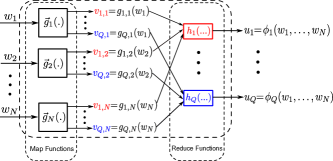
Figure 1: Illustration of a two-stage distributed computing framework. The overall computation is decomposed into computing a set of Map and Reduce functions.

We perform the above computation using $K$ distributed computing servers, labelled by Server $1,$ $\ldots,$ Server $K$. Here the number of servers $K$ is a design parameter and can be an arbitrary positive integer. The chosen $K$ servers carry out the computation in three phases: Map, Shuffle and Reduce.

Map Phase. In the Map phase, each server maps a subset of input files. For each $k\in\{1,\ldots,K\}$, we denote the indices of the files mapped by Server $k$ as ${\cal M}_{k}$, which is a design parameter. Each file is mapped by at least one server, i.e., $\underset{k=1,\ldots,K}{\cup}\mathcal{M}_{k}=\{1,\ldots,N\}$. For each $n$ in $\mathcal{M}_{k}$, Server $k$ computes the Map function $\vec{g}_{n}(w_{n})\!=\!(v_{1,n},\ldots,v_{Q,n})$.

Definition 1 (Peak Computation Load).

We define the peak computation load, denoted by $p$, $0\leq p\leq 1$, as the maximum number of files mapped at one server, normalized by the number of files $N$, i.e., $p\triangleq\frac{\max\limits_{k=1,\ldots,K}|{\cal M}_{k}|}{N}$. $\hfill\Diamond$

We assume that all servers are homogeneous and have the same processing capacity. The average time a server spends in the Map phase is linearly proportional to the number of Map functions it computes, i.e., the average time for a server to compute $n$ Map functions is $c_{\textup{m}}\frac{n}{N}$, for some constant $c_{\textup{m}}>0$. Also, since the servers compute their assigned Map functions simultaneously in parallel, we define the Map time, denoted by $T_{\textup{map}}$, as the average time for the server mapping the most files to finish its computations, i.e.,

$$T_{\textup{map}}=\max\limits_{k=1,\ldots,K}c_{\textup{m}}\tfrac{|{\cal M}_{k}|}{N}=c_{\textup{m}}p.$$ (3)

The minimum possible Map time can be arbitrarily close to $0$, assuming $N$ is large. This minimum Map time can be achieved by using a large number of servers, and letting the $N$ Map tasks be uniformly assigned to these servers without repetition.

Shuffle Phase. We assign the tasks of computing the $Q$ output functions across the $K$ servers, and denote the indices of the output functions computed by Server $k$, $k=1,\ldots,K$, as $\mathcal{W}_{k}$, which is also a design parameter. Each output function is computed exactly once at some server, i.e., 1) $\underset{k=1,\ldots,K}{\cup}{\cal W}_{k}=\{1,\ldots,Q\}$, and 2) ${\cal W}_{j}\cap{\cal W}_{k}=\varnothing$ for $j\neq k$.

To compute the output value $u_{q}$ for some $q\in\mathcal{W}_{k}$, Server $k$ needs the intermediate values that are not computed locally in the Map phase, i.e., $\{v_{q,n}:q\in\mathcal{W}_{k},n\notin\mathcal{M}_{k}\}$. After the Map phase, the $K$ server proceed to exchange the needed intermediate values for reduction. We formally define a shuffling scheme as follows:

• Each server $k$, $k\in\{1,\ldots,K\}$, creates a message $X_{k}$ as a function of the intermediate values computed locally in the Map phase, i.e., $X_{k}=\psi_{k}\left(\{\vec{g}_{n}:n\in\mathcal{M}_{k}\}\right)$, and multicasts it to a subset of $1\leq j\leq K-1$ nodes.

Definition 2 (Communication Load).

We define the communication load, denoted by $L$, $0\leq L\leq 1$, as the total number of bits communicated by all server in the Shuffle phase, normalized by $QNT$ (which equals the total number of bits in all intermediate values $\{v_{q,n}:q\in\{1,\ldots,Q\},n\in\{1,\ldots,N\}\}$). $\hfill\Diamond$

For some constant $c_{\textup{s}}>0$, we denote the bandwidth of the shared link connecting the servers as $1/c_{\textup{s}}$. Thus given a communication load of $L$, the Shuffle time, denoted by $T_{\textup{shuffle}}$, is defined as

$$T_{\textup{shuffle}}=c_{\textup{s}}L.$$ (4)

The minimum possible Shuffle time is $0$. It can be achieved by having each of the servers assigned to compute the Reduce functions map all $N$ files locally.

Reduce Phase. Server $k$, $k\in\{1,\ldots,K\}$, uses the local Map results $\{\vec{g}_{n}:w_{n}\in\mathcal{M}_{k}\}$ and the received messages $X_{1},\ldots,X_{K}$ in the Shuffle phase to construct the inputs to the assigned Reduce functions in $\mathcal{W}_{k}$, and computes the output value $u_{q}=h_{q}(v_{q,1}\ldots v_{q,N})$ for all $q\in\mathcal{W}_{k}$.

Similar to the computations of the Map functions, the average time for a server to compute $q$ Reduce functions is $c_{\textup{r}}q$, for some constant $c_{\textup{r}}>0$. The servers compute their assigned Reduce functions simultaneously in parallel. We define the Reduce time, denoted by $T_{\textup{reduce}}$, as the average time for the server reducing the most output functions to finish its computations, i.e.,

$$T_{\textup{reduce}}=c_{\textup{r}}\underset{k=1,\ldots,K}{\max}|{\cal W}_{k}|.$$ (5)

The minimum Reduce time equals $c_{\textup{r}}$. To minimize the Reduce time, we need at least $Q$ servers, and each computing a unique Reduce function.

In this setting, we are interested in designing distributed computing schemes, which includes the selection of $K$, the assignment of the Map tasks $\boldsymbol{{\cal M}}\triangleq({\cal M}_{1}\ldots,{\cal M}_{K})$, the assignment of the Reduce tasks $\boldsymbol{{\cal W}}\triangleq({\cal W}_{1}\ldots,{\cal W}_{K})$, and the design of the data shuffling scheme, in order to minimize the overall execution time to accomplish the distributed computing tasks.

Specifically, the overall execution time is the total amount of time spent executing the above three phases of the computation. In this paper, we consider the following two types of implementations.

1. Sequential Implementation. For the sequential implementation, the three phases take place one after another sequentially, e.g., the Shuffle phase does not start until all servers have completed their Map computations. In this case, the overall execution time $T_{\textup{sequential}}=T_{\textup{map}}+T_{\textup{shuffle}}+T_{\textup{reduce}}$.

2. Parallel Implementation. For the parallel implementation, the Shuffle phase happens in parallel with the Map phase, i.e., a server communicates a message as soon as the intermediate values needed to construct the message is calculated locally from the Map functions. In this case, the overall execution time becomes $T_{\textup{parallel}}=\max\{T_{\textup{map}},T_{\textup{shuffle}}\}+T_{\textup{reduce}}$.

To design the optimal distributed computing scheme that minimizes the execution time while using as few servers as possible, we need to answer the following questions:

• What is the minimum possible execution time?

• What is the minimum number of servers needed to achieve the minimum possible execution time?

• How to place the Map, Reduce tasks and design the data shuffling scheme to achieve the minimum execution time?

To answer these questions, we formulate them into the following problem:

Problem 1 (Optimal Resource Allocation).

Consider a computing task with parameters $Q$ and $N$. Given a certain number of servers $K$, a Map task assignment $\boldsymbol{{\cal M}}$ and a Reduce task assignment $\boldsymbol{{\cal W}}$ on these servers, we say a shuffling scheme is valid if, for any possible outcomes of the intermediate values $v_{q,n}$, each server can decode all its needed intermediate values based on the values that are locally computed in the map phase and the messages received during the shuffle phase.

Suppose we always use valid shuffling schemes with minimum shuffling time. We denote the resulting execution times given $K$, $\boldsymbol{{\cal M}}$ and $\boldsymbol{{\cal W}}$ by $T^{*}_{\textup{sequential}}(K,\boldsymbol{{\cal M}},\boldsymbol{{\cal W}})$ and $T^{*}_{\textup{parallel}}(K,\boldsymbol{{\cal M}},\boldsymbol{{\cal W}})$. Assuming $N$ is large, we aim to find the minimum execution times over all possible designs, which can be rigorously defined as follows:

$$T^{*}_{\textup{sequential}} =\inf_{K,\boldsymbol{{\cal M}},\boldsymbol{{\cal W}}}{T^{*}_{\textup{sequential}}(K,\boldsymbol{{\cal M}},\boldsymbol{{\cal W}})},$$ (6)

$$T^{*}_{\textup{parallel}} =\inf_{K,\boldsymbol{{\cal M}},\boldsymbol{{\cal W}}}{T^{*}_{\textup{parallel}}(K,\boldsymbol{{\cal M}},\boldsymbol{{\cal W}})}.$$ (7)

We are also interested in finding the minimum number of servers required to exactly achieve the minimum execution time for large $N$, denoted by $K^{*}_{\textup{sequential}}$ and $K^{*}_{\textup{parallel}}$, defined as follows

$$K^{*}_{\textup{sequential}} =\min\{K\in\mathbb{N}\ |\ \min_{\boldsymbol{{\cal M}},\boldsymbol{{\cal W}}}T^{*}_{\textup{sequential}}(K,\boldsymbol{{\cal M}},\boldsymbol{{\cal W}})=T^{*}_{\textup{sequential}}\},$$ (8)

$$K^{*}_{\textup{parallel}} =\min\{K\in\mathbb{N}\ |\ \min_{\boldsymbol{{\cal M}},\boldsymbol{{\cal W}}}T^{*}_{\textup{parallel}}(K,\boldsymbol{{\cal M}},\boldsymbol{{\cal W}})=T^{*}_{\textup{parallel}}\}.$$ (9)

If the minimum in any of the above equations does not exist, we say the corresponding $T^{*}_{\textup{sequential}}$ or $T^{*}_{\textup{parallel}}$ can not be achieved using finite number of servers.

Besides, we want to find the optimal computing schemes that minimizes the execution time while using the minimum number of servers. Specifically, for each implementation, we want to construct a Map task assignment $\boldsymbol{\mathcal{M}}$, a reduce task assignment $\boldsymbol{\mathcal{W}}$, and a valid shuffling scheme design, that achieve the minimum execution time using the minimum number of servers. $\hfill\Diamond$

In this paper, we answer all the questions mentioned in the above problem. Interestingly, some of the answers match the intuition and some do not. For example, the coding gain in our proposed optimal scheme is obtained through coded multicasting, which agrees with the intuition. However, counter intuitively, the optimal scheme requires a non-symmetric design, where the servers are classified into two groups. One group is only assigned Map and Reduce tasks, focusing on computing the output functions; while the other group only does Map and Shuffle, focusing on delivering the intermediate results and exploiting the multicast opportunity. Also, the intuition may suggest that by using more servers, we may always be able to further reduce the execution time. However, we show that in most cases, the minimum execution time can be exactly achieved using finitely many servers, and the minimum execution time can not be further reduced after the number of servers passes a threshold.

III Main Results

For the sequential implementation, we characterize the minimum execution time $T_{\textup{sequential}}^{*}$ and the minimum number of servers to achieve $T_{\textup{sequential}}^{*}$ in the following theorem.

Theorem 1 (Sequential Implementation).

For a distributed computing application that computes $Q$ output functions, $T_{\textup{sequential}}^{*}$ defined in Problem 1 is given by

$$T_{\textup{sequential}}^{*} =c_{\textup{m}}\tfrac{r^{*}}{Q}+c_{\textup{s}}\tfrac{Q-r^{*}}{Q(r^{*}+1)}+c_{\textup{r}},$$ (10)

where $r^{*}$ is defined as follows:

$$r^{*}=\max\underset{r\in\{0,1\ldots,Q\}}{\textup{argmin}}\ c_{\textup{m}}\frac{r}{Q}+c_{\textup{s}}\frac{Q-r}{Q(r+1)}.$$ (11)

We can show that the above execution time can be exactly achieved using a finite number of servers if and only if $r^{*}\neq 0$. For $r^{*}\neq 0$, $K_{\textup{sequential}}^{*}$ defined in Problem 1 is given by

$$K_{\textup{sequential}}^{*}=\begin{cases}Q+\lceil\tfrac{Q}{r^{*}}\rceil,&0<r^{*}<Q,\\ Q,&r^{*}=Q.\end{cases}$$ (12)

Remark 1.

The above theorem generalizes the prior works on coded distributed computing, [11, 10, 12, 13], by allowing the flexibility of using arbitrary number of servers and arbitrary reduce task assignments on the servers. In prior works, it is assumed that all the $Q$ Reduced tasks are uniformly assigned to all the servers. In this paper, we will see that by focusing on the execution time and allowing using arbitrary number of servers, the optimal scheme naturally requires a certain Reduce task assignment, where each server either reduce $1$ function, or does not reduce at all. To simplify the discussion, we refer to the servers that are assigned Reducing tasks as solvers, and we refer to the rest of the servers as helpers.

Remark 2.

To achieve the above minimum execution time, we propose a distributed computing scheme, where each server maps no more than $\frac{r^{*}}{Q}$ fraction of the files in the database, with communication load of $\frac{Q-r^{*}}{Q(r^{*}+1)}$. In the proposed achievability scheme, we will see each file repetitively mapped on $r^{*}$ solvers. Having this redundancy in the Map phase has two advantages: first of all, more computation enhances the local availability of the intermediate values, thus each solver only needs values from $1-\frac{r^{*}}{Q}$ fraction of the files from the the shuffling phase; secondly, mapping the same file at multiple servers allows delivering intermediate values through coded multicasting, and a coding gain of $r^{*}+1$ is achieved in the proposed delivery scheme.

Remark 3.

Similar to the prior works [11, 10, 12, 13], the trade off between computation load and communication load can be established, and the above theorems demonstrate how the optimal peak computation load can be chosen based on the trade off.

Remark 4.

We prove the exact optimality of the proposed scheme through a matching information theoretic converse, which is provided in section V. We observe that in most cases, using a finite number of servers is sufficient to exactly achieve the lower bound of the minimum execution time, which means that the execution time cannot be further reduced by using more servers than the provided $K_{\textup{sequential}}^{*}$. This is due to the fact that the coded multicasting opportunity, which is essential to achieving the minimum communication load, relies on mapping the files repetitively on the solvers. Because the total number of Reduce functions is fixed, the number of solvers is upper bounded by $Q$ even if we use infinitely many servers. Consequently, by using a large number of servers, reducing the peak computation load on the solvers will inevitably reduce the number of times that each file is repetitively mapped on the solvers, which consequently hurts the coded multicasting opportunity and increases the communication load. Hence, the entire benefit of using more than $Q$ servers is to reduce the computation load of the helpers, until the computation load of the solvers becomes the bottleneck. Further increasing the number of servers will not affect the computation-communication trade-off.

Conversely, Theorem 1 also indicates that, when using fewer servers than the suggested minimum number ($K_{\textup{sequential}}^{*}$), the resulting computing scheme must be strictly suboptimal. This is due to the fact that only the helpers can fully utilize the coded multicasting opportunity during the shuffling phase. Hence, to achieve the minimum communication load, no shuffling job should be handled by the solvers, and we need sufficient helpers to map enough files in order to obtain enough information to support the shuffling phase, without becoming the bottleneck of the peak computation load.

Remark 5.

From theorem 1, we observe that the optimal solution always requires using at least $Q$ servers, which is because any computing scheme having a server reducing more that one function is strictly suboptimal (will be proved later), so at least $Q$ solvers are needed to compute all the Reduce functions.

In addition, we note that $K^{*}_{\textup{sequential}}$, is a decreasing function of $r^{*}$, and consequently an increasing function of $\frac{c_{\textup{m}}}{c_{\textup{s}}}$, which can be explained as follows: When $\frac{c_{\textup{m}}}{c_{\textup{s}}}$ increases, the computation time for mapping one file becomes relatively larger, therefore it is better to pick a computing scheme with larger communication load and smaller computation load. To reduce the computation load, $r^{*}$, the number of times each file is repetitively mapped on all the solvers, should be decreased. As a result, the peak computation load on the helpers also decreases, and thus more helpers are needed to make sure that each file needed for the shuffling phase is mapped on at least one helper.

Remark 6.

If we ignore the integrality constraint, $r^{*}$ and $K_{\textup{sequential}}^{*}$ can be approximated as follows:

$$r^{*} \approx\sqrt{(Q+1)\frac{c_{\textup{s}}}{c_{\textup{m}}}}-1\approx\sqrt{Q\frac{c_{\textup{s}}}{c_{\textup{m}}}}$$ (13)

$$K_{\textup{sequential}}^{*} \approx Q+Q/(\sqrt{(Q+1)\frac{c_{\textup{s}}}{c_{\textup{m}}}}-1)\approx Q+\sqrt{Q\frac{c_{\textup{m}}}{c_{\textup{s}}}}.$$ (14)

Interestingly, $r^{*}$ is approximately proportional to the square root of $\frac{c_{\textup{s}}}{c_{\textup{m}}}$, while the number of helpers (i.e., $K^{*}_{\textup{sequential}}-Q$) is inversely proportional to the square root of $\frac{c_{\textup{s}}}{c_{\textup{m}}}$. Hence if the computation time of mapping one file is increased by $4$ times, $r^{*}$ should be halved, and the number of helpers should be doubled.

We have the following explanation: In the optimal computing scheme proposed in this paper, the computation time is proportional to $c_{\textup{m}}r$, and the communication time is approximately $c_{\textup{s}}/r$, where $r$ is the number of times each file is repetitively mapped on all solvers. To minimize the total execution time, the design parameter should balance the time used in these two phases, which results that $r^{*}$ should be approximately proportional to the square root of $\frac{c_{\textup{s}}}{c_{\textup{m}}}$. Besides, in most cases the helpers should map all files in the database in order to execute the shuffling functions. Hence the minimum number of helpers (i.e., $K^{*}_{\textup{sequential}}-Q$) should be inversely proportional to the computation load, which should consequently be inversely proportional to the square root of $\frac{c_{\textup{s}}}{c_{\textup{m}}}$.

Remark 7.

As we have discussed, achieving the minimum possible communication load relies on exploiting local availabilities and allowing coded multicasting. As a comparison, we consider computing designs where the opportunity of multicasting during the shuffling phase is not utilized, i.e., the shuffling phase is uncoded. The minimum execution time is given as follows:

$$T_{\textup{sequential, uncoded}}^{*} =\min_{r\in\{0,Q\}}c_{\textup{m}}\tfrac{r}{Q}+c_{\textup{s}}({1-\frac{r}{Q}})+c_{\textup{r}}$$ (15)

$$=\min\{c_{\textup{m}},c_{\textup{s}}\}+c_{\textup{r}}.$$ (16)

The above execution time can be achieved using uncoded computing scheme with finite number of servers if and only if $c_{\textup{m}}\leq c_{\textup{s}}$, and the minimum needed number of server in this case equals $Q$.

Compared to the uncoded scheme, a large coding gain that scales with the size of the problem can be achieved by exploiting coded multicasting opportunities during the shuffling phase. For example, when $c_{m}=c_{s}$, the execution time for the Map and Shuffle phase of the optimal coded scheme grows as $\Theta(Q^{-\frac{1}{2}})$, while the execution time of the uncoded scheme remains constant.

The two schemes also requires different number of servers to achieve the minimum execution time. For the uncoded computing scheme, at most $Q$ servers are needed to achieve the minimum cost, unless the computing power of $Q$ servers are not sufficient to map the entire database; while for the coded computing scheme, in most cases more that $Q$ servers are needed to achieve the minimum execution time. This is due to the fact that in the coded computing scheme, the Reduce tasks and the shuffling jobs are handled by disjoint groups of servers in order to fully maximize the coding gain, and hence extra servers are needed to optimize the performance. However in the uncoded scheme, the only use of non-solver nodes is to provide extra computing power. Hence when $Q$ servers are sufficient to map the entire database, using more servers does not reduce the execution time.

For the parallel implementation, we characterize the minimum execution time, and the minimum number of servers to achieve $T_{\textup{sequential}}^{*}$ in the following theorem

Theorem 2 (Parallel Implementation).

For a distributed computing application that computes $Q$ output functions, $T_{\textup{parallel}}^{*}$ defined in Problem 1 is given by

$$T_{\textup{parallel}}^{*} =\max\{c_{\textup{m}}\tfrac{r^{*}}{Q},c_{\textup{s}}\cdot\textup{Conv}(\tfrac{Q-r^{*}}{Q(r^{*}+1)})\}+c_{\textup{r}},$$ (17)

where $\textup{Conv}(f(\cdot))$ denotes the lower convex envelope of points $\{(r,f(r))\ |\ r\in\{0,1,...,Q\}\}$, and $r^{*}$ is defined as follows:

$$r^{*}=\underset{0\leq r\leq Q}{\textup{argmin}}\ \max\{c_{\textup{m}}\tfrac{r}{Q},c_{\textup{s}}\cdot\textup{Conv}(\tfrac{Q-r}{Q(r+1)})\}.$$ (18)

We can show that the above execution time can be exactly achieved using a finite number of servers, and $K_{\textup{parallel}}^{*}$ defined in Problem 1 is given by

$$K_{\textup{parallel}}^{*}=\begin{cases}Q+\lceil\tfrac{Q}{r^{*}}\rceil,&r^{*}\leq Q-1,\\ Q+\lceil\tfrac{Q(Q-r^{*})}{r^{*}}\rceil,&r^{*}>Q-1.\end{cases}$$ (19)

Remark 8.

The above theorem generalized the prior works [11, 10, 12, 13], by allowing the flexibility of using an arbitrary number of servers and arbitrary Reduce task assignments on the servers. Similar to the sequential implementation, the optimal scheme for parallel implementation also requires a certain Reduce task assignment, where each server either reduces $1$ function or does not reduce at all. Thus, we continue to use the names solvers and helpers for the parallel implementation.

Remark 9.

To achieve the above minimum execution time, we propose a distributed computing scheme, where each server maps no more than $\frac{r^{*}}{Q}$ fraction of the files in the database, with communication load of $\textup{Conv}(\frac{Q-r^{*}}{Q(r^{*}+1)})$. Similar to the sequential case, each file is repetitively mapped $r^{*}$ times. This redundancy enhances the local availability of the intermediate values, and allows delivering intermediate values through coded multicasting. Hence, by following the same argument, we can achieve the same computation-communication trade off achieved by the scheme used in sequential implementations. However, given the same computation-communication trade off, the above theorem indicates that the optimal peak computation load should be chosen differently compared to the sequential case, in order to minimum the execution time for parallel implementation.

Remark 10.

We prove the exact optimality of the proposed scheme through a matching information theoretic converse, which is provided in section V. We note that for parallel implementation, using finite number of servers is sufficient to exactly achieve the minimum execution time. Conversely, the statement in theorem 1 also indicates that when using less servers than the suggested minimum number ($K_{\textup{parallel}}^{*}$), the resulting computing scheme must be strictly suboptimal. Both statements can be understood exactly the same way as discussed for the sequential implementation.

Remark 11.

From theorem 2, we observe that the optimal solution always requires using at least $Q$ servers. In addition, we note that $K^{*}_{\textup{parallel}}$, is a decreasing function of $r^{*}$, and consequently an increasing function of $\frac{c_{\textup{m}}}{c_{\textup{s}}}$. Both observations can be understood exactly the same way as discussed for the sequential implementation.

Remark 12.

If we ignore the integrality constraint, $r^{*}$ and $K_{\textup{parallel}}^{*}$ can be approximated as follows:

$$r^{*}\approx\sqrt{Q\frac{c_{\textup{s}}}{c_{\textup{m}}}+(\frac{c_{\textup{s}}/c_{\textup{m}}+1}{2})^{2}} -\frac{c_{\textup{s}}/c_{\textup{m}}+1}{2}\approx\sqrt{Q\frac{c_{\textup{s}}}{c_{\textup{m}}}}$$ (20)

$$K_{\textup{parallel}}^{*}\approx Q+Q/r^{*} \approx Q+\sqrt{Q\frac{c_{\textup{m}}}{c_{\textup{s}}}}.$$ (21)

Similar to the sequential case, $r^{*}$ is approximately proportional to the square root of $\frac{c_{\textup{s}}}{c_{\textup{m}}}$, while the number of helpers (i.e., $K^{*}_{\textup{parallel}}-Q$) is inversely proportional to the square root of $\frac{c_{\textup{s}}}{c_{\textup{m}}}$. Both approximations can be explained through the same arguments used for the sequential implementation.

Remark 13.

We consider the minimum execution time of the uncoded scheme, which is given as follows:

$$T_{\textup{parallel, uncoded}}^{*} =\min_{r\in[0,Q]}\max\{c_{\textup{m}}\tfrac{r}{Q},c_{\textup{s}}({1-\frac{r}{Q}})\}+c_{\textup{r}}$$ (22)

$$=\frac{c_{\textup{m}}c_{\textup{s}}}{c_{\textup{m}}+c_{\textup{s}}}+c_{\textup{r}}.$$ (23)

The above execution time can be achieved using $K_{\textup{parallel, uncoded}}^{*}=\max\{Q,\lceil\frac{Q}{r^{*}}\rceil\}$ servers.

Compared to the uncoded scheme, a large coding gain that scales with the size of the problem is achieved using the proposed coded scheme. For example, when $c_{m}=c_{s}$, the execution time for the Map and Shuffle phase of the optimal coded scheme grows as $\Theta(Q^{-\frac{1}{2}})$, while the execution time of the uncoded scheme remains constant.

The two schemes also requires different number of servers to achieve the minimum execution time. For the uncoded scheme, at most $Q$ servers are needed to achieve the minimum cost, unless the computing power of $Q$ servers are not sufficient to map the entire database; while for the coded computing scheme, in most cases more that $Q$ servers are needed to achieve the minimum execution time. This is due to the fact that uncoded scheme failed to exploit the coded multicast opportunity, as explained in Remark 7.

IV Achievability Schemes

In this section, we construct achievability schemes that achieve the minimum execution time mentioned in Section III, using the minimum number of servers. We start by giving an illustrative example on how to build an optimal scheme for sequential implementation given a specific set of values of problem parameters. Then we proceed to present the optimal achievability scheme for general parameters. The optimal achievability schemes for the parallel implementation is described in Appendix A.

IV-A Illustrative Example

We present an illustrative example of the optimal achievability scheme for a given set of parameters: $N=6$, $Q=3$, $c_{\textup{m}}=1$, $c_{\textup{s}}=2$ and $c_{\textup{r}}=1$. According to Theorem 1, we choose design parameter $r^{*}=2$ and use $K^{*}_{\textup{sequential}}=5$ servers. We let servers $1,2$, and $3$ reduce functions $1,2$, and $3$, respectively.

Figure 2: Illustration of the optimal achievability scheme for $N=6$, $Q=3$, $c_{\textup{m}}=1$, $c_{\textup{s}}=2$ and $c_{\textup{r}}=1$.

Map Phase Design. We let the Map task assignment to the $5$ users be $\mathcal{M}_{1}=\{1,2,3,4\}$, $\mathcal{M}_{2}=\{3,4,5,6\}$, $\mathcal{M}_{3}=\{1,2,5,6\}$, $\mathcal{M}_{4}=\{1,3,5\}$, and $\mathcal{M}_{5}=\{2,4,6\}$. Here each solver, i.e. users in $\{1,2,3\}$, maps $\frac{4}{6}=\frac{r^{*}}{Q}$ fraction of the file, and each helper maps $\frac{3}{6}<\frac{r^{*}}{Q}$ fraction of the files. Hence the peak computation load equals $\frac{4}{6}=\frac{r^{*}}{Q}$.

Shuffle Phase Design. After the map phase, user $4$ multicast the message $v_{5,1}\oplus v_{1,2}\oplus v_{3,3}$, and user $5$ multicast the message $v_{6,1}\oplus v_{2,2}\oplus v_{4,3}$. The normalized communication load equals $\frac{2}{18}=\tfrac{Q-r^{*}}{Q(r^{*}+1)}$. Since node $1$ knows $v_{1,2}$ and $v_{3,3}$, he can decode $v_{5,1}$ from the message multicasted by user $4$. Similarly, he can also decode $v_{6,1}$ from the other message. Because $v_{1,1},...,v_{4,1}$ are already locally computed by user $1$, the Reduce function $1$ can be executed after the shuffle phase. Same argument holds for the other $2$ Reduce functions, hence the computation can be completed after the shuffling.

Note that in the above example, each server computes at most $1$ Reduce function. Hence the reduce time equals $1$. Consequently, the total execution time for sequential implementation equals $1\cdot\frac{4}{6}+2\cdot\frac{2}{18}+1=c_{\textup{m}}\frac{r^{*}}{Q}+c_{\textup{s}}\frac{Q-r^{*}}{Q(r^{*}+1)}+c_{\textup{r}}$, which can be verified to be equal to the minimum execution time $T^{*}_{\textup{sequential}}$ given in Theorem 1.

IV-B General Description for Sequential Implementation

We consider a general computing task with $Q$ Reduce functions, parameters $c_{\textup{m}}$, $c_{\textup{s}}$, $c_{\textup{r}}$, and sufficiently large $N$. We first compute the design parameter $r^{*}$ as specified in Theorem 1. Depending on the value of $r^{*}$, we design the achievability scheme as follows.

IV-B1 $r^{*}\in\{1,...,Q-1\}$

We use $K=K^{*}_{\textup{sequential}}$ servers as suggested in Theorem 1. Note that $K^{*}_{\textup{sequential}}\geq Q$ always holds, we let nodes $1,2,...,Q$ reduce functions $1,2,...,Q$ respectively.

Map Phase Design. Assuming $N$ is large, we evenly partition the dataset into $(K-Q)\binom{Q}{r^{*}}$ disjoint subsets. We bijectively map these subsets, to tuples of a subset of $r^{*}$ solvers and a helper. Rigorously, we map the subset of files to the following set: $\{(i,\mathcal{A})\ |\ i\in\{Q+1,...,K\},\mathcal{A}\subseteq\{1,...,Q\},|\mathcal{A}|=r^{*}\}$. We denote the subset of files that is mapped to $(i,\mathcal{A})$ by $\mathcal{B}_{i,\mathcal{A}}$.

We let each solver $k\in\{1,...,Q\}$ map all subsets of files $\mathcal{B}_{i,\mathcal{A}}$ satisfying $k\in\mathcal{A}$, and we let each helper $k\in\{Q+1,...,K\}$ map all subsets $\mathcal{B}_{k,\mathcal{A}}$. Each solver maps $\frac{\binom{Q-1}{r^{*}-1}(K-Q)}{\binom{Q}{r^{*}}(K-Q)}=\frac{r^{*}}{Q}$ fraction of the files, and each helper maps $\frac{\binom{Q}{r^{*}}}{\binom{Q}{r^{*}}(K-Q)}=\frac{1}{K-Q}\leq\frac{r^{*}}{Q}$ fraction of the files. Hence, the computation time of this given Map phase design equals $c_{\textup{m}}\frac{r^{*}}{Q}$.

Shuffle Phase Design. We group all the intermediate values for a Reduce function $q$ from all files in $\mathcal{B}_{i,\mathcal{A}}$ into a single variable, and denote it by $V_{i,\mathcal{A},q}$. At the shuffling phase, each helper from $i\in\{Q+1,...,K\}$ will multicast the following messages: For each subset of $r^{*}+1$ solvers, denoted by $\mathcal{S}$, helper $i$ multicasts $Y_{i,\mathcal{S}}\triangleq\oplus_{k\in\mathcal{S}}{V_{i,\mathcal{S}\backslash\{k\},k}}$ to all the solvers in $\mathcal{S}$. The normalized communication load equals $\frac{\binom{Q}{r^{*}+1}(K-Q)}{\binom{Q}{r^{*}}(K-Q)Q}=\frac{Q-r^{*}}{Q(r^{*}+1)}$. Hence, the computation time of this given Shuffle phase design equals $c_{\textup{s}}\frac{Q-r^{*}}{Q(r^{*}+1)}$.

Now we prove the validity of the above scheme: For each subset $\mathcal{A}\subseteq\{2,...,Q\}$ of size $r^{*}$ and for each $i\in\{Q+1,...,K\}$, server $1$ can decode $V_{i,\mathcal{A},1}$ from $Y_{i,\mathcal{S}\cup\{1\}}$. Combining with the intermediate values that are computed locally on server $1$, the reduce function $1$ can be executed after the shuffle phase. Same argument holds for the other $Q-1$ Reduce functions, hence the proposed shuffling scheme is valid.

Remark 14.

Note that if we view all the helpers as $1$ super node, the node maps all the files and broadcasts all messages during the shuffle phase. By viewing the super node as the server and the solvers as the users, we recover the caching scheme proposed in [16]. In our proposed distributed computing scheme, we split the work in the map phase for the super node onto multiple nodes, in order to ensure the peak computation load is not bottlenecked by the Map tasks executed at these helpers.

IV-B2 $r^{*}=0$

In this case, Theorem 1 states that $T^{*}_{\textup{sequential}}$ cannot be exactly achieved using finite number of servers. Hence we consider picking a parameter $K$ as large as possible, and use $K$ servers for the achievability scheme. We let nodes $1,2,...,Q$ reduce functions $1,2,...,Q$ respectively, and not being assigned any Map tasks. Assuming $N$ is large, we evenly partition the dataset into $K-Q$ subsets of files, and we let each helper disjointly maps one subset. The peak computation load consequently equals $\frac{1}{K-Q}$, which is negligible if $K$ is sufficiently large. Hence the Map Phase design requires a computation time of $c_{\textup{m}}\cdot 0=c_{\textup{m}}\cdot\frac{r^{*}}{Q}$.

At the shuffling phase, note that each the intermediate value is computed by exactly one helper, we simply let all the helpers unicast each intermediate value to the solver that requires the value to execute the reduce function. Because each intermediate value is unicast exactly once, the normalized communication load equals $1$ and the communication time equals $c_{\textup{s}}\cdot 1=c_{\textup{s}}\frac{Q-r^{*}}{Q(r^{*}+1)}$.

IV-B3 $r^{*}=Q$

In this case, $K^{*}_{\textup{sequential}}=Q$. We simply use $Q$ servers, each reducing one function, and maps the entire database. The peak computation load equals $1$, hence the computation time equals $c_{\textup{m}}\cdot 1=c_{\textup{m}}\cdot\frac{r^{*}}{Q}$. Note that each server obtains all the needed intermediate values after the Map phase, no communication is required in the shuffling phase. Hence the communication time equals $c_{\textup{s}}\cdot 0=c_{\textup{s}}\frac{Q-r^{*}}{Q(r^{*}+1)}$.

In all the above cases, each server reduces at most one function. Hence our proposed achievability scheme always achieve a reduce time of $c_{\textup{r}}$. Besides, in all the cases, the achievability scheme uses $K^{*}_{\textup{sequential}}$ servers (or sufficiently many servers if $K^{*}_{\textup{sequential}}$ does not exist), achieves a computation time of $c_{\textup{m}}\cdot\frac{r^{*}}{Q}$ and a communication time of $c_{\textup{s}}\frac{Q-r^{*}}{Q(r^{*}+1)}$. The total execution time always equals $T^{*}_{\textup{sequential}}=c_{\textup{m}}\cdot\frac{r^{*}}{Q}+c_{\textup{s}}\frac{Q-r^{*}}{Q(r^{*}+1)}+c_{\textup{r}}$. Hence, our proposed scheme always achieves the $T^{*}_{\textup{sequential}}$ and $K^{*}_{\textup{sequential}}$ stated in Theorem 1.

Remark 15.

Interestingly, in the proposed optimal computing scheme, the minimum cost is achieved by completely separating the Reduce tasks and the shuffle jobs onto different servers. Because no solver in the proposed scheme are responsible for multicasting messages in the delivery phase, the Map tasks on the solvers can be perfectly designed in order to fully exploiting the multicast opportunity, without having to considerate the encodability constraint.

V Converse

In this section, we derive matching converses that shows the optimality of the proposed computation scheme. We also show that our proposed optimal scheme uses the minimum possible number of nodes to achieve the minimum execution time.

V-A Key Lemma

Before deriving the exact converse for each implementation, we first prove the following key lemma, that applies for both sequential and parallel implementations. The lemma lower bounds the shuffling time given an arbitrary Map and Reduce task allocation:

Lemma 1 (Converse Bound for Communication Load).

Consider a distributed computing task with $N$ files and $Q$ Reduce functions, and a given map and reduce design that uses $K$ nodes. For any integers $s,d$, let $a_{s,d}$ denotes the number of intermediate values that are available at $s$ nodes, and required by (but not available at) $d$ nodes. The following lower bound on the communication load holds:

$$L\geq\frac{1}{QN}\sum_{s=1}^{K}\sum_{d=1}^{K-s}a_{s,d}\frac{d}{s+d-1}$$ (24)

Remark 16.

Prior to this work, several bounding techniques have been proposed for coded distributed computing and coded caching with uncoded prefetching [10, 12, 13, 17, 18, 19] . All of them can be derived as special cases of the above simple lemma.

Remark 17.

Although we assume that each server sends messages independently during the shuffling phase, the above lemma can be easily generalized to computing models where the data shuffling process can be carried out in multiple rounds and dependency between messages are allowed. We can prove that even multiple round communication is allowed, the exactly same lower bound stated in Lemma 1 still holds. Consequently, requiring the servers communicating independently does not induce any cost in the total execution time.

We postpone the proof of Lemma 1 to Appendix B, and in this section, we assume the correctness of this lemma and prove the optimality of the proposed schemes based on that.

V-B Converse Bounds for Sequential Implementation

Now we use Lemma 1 to prove a matching converse for Theorem 1, which is equivalent to prove the following two statements:

1. The execution time of any coded computing scheme for a distributed computing task with $N$ files and $Q$ Reduce functions with sequential implementation is at least $T^{*}_{\textup{sequential}}$.

2. Any computing scheme that arbitrarily closely achieve a execution time of $T^{*}_{\textup{sequential}}$ uses at least $K^{*}_{\textup{sequential}}$ servers.

First of all, note that for any coded computing scheme, we can construct an alternative valid scheme with the same computation load and communication load, but each server only reduces at most $1$ function. The construction is given as follows:

Given the computing scheme, for each server $k$ that reduce at least $1$ functions, let $q_{k}$ denotes the number of functions reduced by this server. Make $q_{k}-1$ extra copies of this server mapping the same set of files, but not responsible for any shuffling job, and let each of these $q_{k}$ users reduce only one of the $q_{k}$ functions originally assigned to server $k$. If all map, shuffle, and reduce phases for the other servers remain the same, each additional server can still obtain enough information to execute the reduce function. Besides, the Map time and the Shuffle time remain the same, but each server in the new computing scheme only reduces at most $1$ function.

Consequently, for any computing scheme that assigns more than $1$ function to any single server, we can find a further optimized scheme with a strict improvement in the execution time of at least $c_{\textup{r}}$. Hence any such scheme can not achieve the minimum possible execution time. So to prove a matching converse for Theorem 1, it is sufficient to focus on computing schemes where each server reduces at most one function.

We consider an arbitrary computing scheme that maps $N$ files, uses $K$ servers and reduces $Q$ functions. Without loss of generality, we assume servers in $\{1,...,Q\}$ are assigned Reduce tasks.

We first derive a lowerbound on the communication load by enhancing the computing system: We view the servers in $Q+1,...,K$ as a super node, that maps all files that are mapped by these servers, and broadcast all messages that are broadcast by these servers during the shuffling phase. It is easy to verify that by enhancing the computing system in this way, all solvers are still able to execute the reduce function, and the total communication load does not increase.

We then apply Lemma 1 on the enhanced computing system. Let $a_{j,0}$ denotes the number of files that are mapped by $j$ solvers, but not mapped by the super node, and let $a_{j,1}$ be the number of files that are mapped by $j$ solvers, and mapped by the super node. From Lemma 1, the communication load is lower bounded by the following inequality:

$$L\geq\frac{1}{QN}\sum_{j=0}^{Q}(Q-j)a_{j,0}\frac{1}{j}+(Q-j)a_{j,1}\frac{1}{j+1}.$$ (25)

Note that the peak computation load is lower bounded by the average computation load on the solvers, thus

$$p\geq\sum_{k=1}^{Q}\frac{|\mathcal{M}_{k}|}{QN}=\frac{1}{QN}\sum_{j=0}^{Q}j(a_{j,0}+a_{j,1}).$$ (26)

Hence, the total execution time is lower bounded by

$$T_{\textup{sequential}}\geq \frac{1}{QN}(\sum_{j=0}^{Q}a_{j,0}(c_{\textup{m}}j+c_{\textup{s}}\frac{Q-j}{j})+a_{j,1}(c_{\textup{m}}j+c_{\textup{s}}\frac{Q-j}{j+1}))+c_{\textup{r}}.$$ (27)

Note that $a_{j,0}$, $a_{j,1}$ are non-negative and satisfy the following equation

$$N=\sum_{j=0}^{Q}(a_{j,0}+a_{j,1}).$$ (28)

Consequently, the minimum value that $T_{\textup{sequential}}$ can take is given by

$$T_{\textup{sequential}}\geq \frac{1}{Q}(\min_{j\in\{0,...,Q\}}\min\{c_{\textup{m}}j+c_{\textup{s}}\frac{Q-j}{j},c_{\textup{m}}j+c_{\textup{s}}\frac{Q-j}{j+1}\})+c_{\textup{r}}$$ (29)

$$= \min_{r\in\{0,...,Q\}}(c_{\textup{m}}\frac{r}{Q}+c_{\textup{s}}\frac{Q-r}{Q(r+1)})+c_{\textup{r}}$$ (30)

$$= T^{*}_{\textup{sequential}},$$ (31)

which proves the first statement.

Let $\mathcal{R}^{*}=\underset{r\in\{0,1,...,Q\}}{\textup{argmin}}(c_{\textup{m}}\frac{r}{Q}+c_{\textup{s}}\frac{Q-r}{Q(r+1)})$, we have $r^{*}=\max\mathcal{R}^{*}$. If $T^{*}_{\textup{sequential}}$ is arbitrarily closely achieved, the Map task assignment of the computation scheme must satisfy that $a_{j,i}\approx 0$ except for $j\in\mathcal{R}^{*}$, and $i=1$ if $j\neq Q$.

We consider the following two possible cases, distinguished by the value of $r^{*}$:

1. If $r^{*}\neq Q$, i.e., $Q\notin\mathcal{R}^{*}$. $a_{j,i}$ can only be non-zero when $i=1$, which means almost all files must be mapped at the super node. Since the equality for (26) must hold in order for a computing scheme to arbitrarily achieve the lower bound of $T_{\textup{sequential}}$, the peak computation load must be no larger than $\frac{r*}{Q}$. Consequently, the minimum number of helpers must be at least $\lceil\frac{1}{p}\rceil=\lceil\frac{Q}{r^{*}}\rceil$ in order for them to map all the files.

Hence, we have

$$K\geq Q+\lceil\frac{Q}{r^{*}}\rceil=K^{*}_{\textup{sequential}}.$$ (32)

Note that if $r^{*}=0$, the minimum execution time can not be achieved using finite number of servers.

2. If $r^{*}=Q$, the required number of servers to achieve $T^{*}_{\textup{sequential}}$ is simply bounded by $Q$, because $Q$ Reduce functions has to be assigned to distinct servers. Hence $K\geq Q=K^{*}_{\textup{sequential}}$.

Hence, the second statement is proved for all possible values of $r^{*}$.

V-C Converse Bounds for Parallel Implementation

Now we use Lemma 1 to prove a matching for Theorem 2, which is equivalent to prove the following two statements:

1. The execution time of any coded computing scheme for a distributed computing task with $N$ files and $Q$ Reduce functions with parallel implementation is at least $T^{*}_{\textup{parallel}}$.

2. Any computing scheme that arbitrarily closely achieve a execution time of $T^{*}_{\textup{parallel}}$ uses at least $K^{*}_{\textup{parallel}}$ servers.

Similar to the sequential case, we can easily show that any computing scheme that assigns more than $1$ Reduce function to any single server can not achieve the minimum possible execution time. So to prove a matching converse, it is sufficient to focus on computing schemes where each server reduces at most one function.

We consider an arbitrary a computing scheme that maps $N$ files, uses $K$ servers and reduces $Q$ functions. Without loss of generality, we assume servers in $\{1,...,Q\}$ are assigned Reduce tasks. Following the same arguments and the same notation used for the sequential case, the following bounds for the communication load and the computation load also hold for sequential implementation:

$$L \geq\frac{1}{QN}\sum_{j=0}^{Q}(Q-j)a_{j,0}\frac{1}{j}+(Q-j)a_{j,1}\frac{1}{j+1},$$ (33)

$$p \geq\frac{1}{QN}\sum_{j=0}^{Q}j(a_{j,0}+a_{j,1}).$$ (34)

Let $\textup{Conv}(f(\cdot))$ denotes the lower convex envelop of points $\{(r,f(r))\ |\ r\in\{0,1,...,Q\}\}$, we have

$$L \geq\frac{1}{N}\sum_{j=0}^{Q}(a_{j,0}+a_{j,1})\frac{Q-j}{Q(j+1)}$$ (35)

$$=\frac{1}{N}\sum_{j=0}^{Q}(a_{j,0}+a_{j,1})\ \textup{Conv}\left(\frac{Q-j}{Q(j+1)}\right).$$ (36)

Note that

$$N=\sum_{j=0}^{Q}(a_{j,0}+a_{j,1}),$$ (37)

and $\frac{Q-j}{Q(j+1)}$ is a decreasing sequence, using Jensen’s inequality, we have

$$L \geq\textup{Conv}\left(\frac{Q-r}{Q(r+1)}\right),$$ (38)

where $r=Qp$.

Consequently,

$$T_{\textup{parallel}} \geq\min_{r\in[0,Q]}\max\{c_{\textup{m}}\frac{r}{Q},\ c_{\textup{s}}\ \textup{Conv}\left(\frac{Q-r}{Q(r+1)}\right)\}+c_{\textup{r}}$$ (39)

$$=T^{*}_{\textup{parallel}},$$ (40)

which proves the first statement.

It is easy to show that the above bound is minimized by a unique value $r^{*}\in(0,Q)$. If $T^{*}_{\textup{parallel}}$ is arbitrarily closely achieved, the equality of the Jensen’s inequality used in (38) must hold. Consequently, the Map task assignment of the computation scheme must satisfy that $a_{j,i}\approx 0$ except for $j=\lfloor r^{*}\rfloor$ or $\lceil r^{*}\rceil$, and $i=1$ if $j\neq Q$.

We consider the following two possible cases, distinguished by the value of $r^{*}$:

1. If $r^{*}\leq Q-1$, $a_{j,i}$ can only be non-zero when $i=1$, which means almost all files must be mapped at the super node. Similar to the sequential case, the minimum number of helpers must be at least $\lceil\frac{1}{p}\rceil=\lceil\frac{Q}{r^{*}}\rceil$ in order for them to map all the files. Hence, we have

$$K\geq Q+\lceil\frac{Q}{r^{*}}\rceil=K^{*}_{\textup{parallel}}.$$ (41)

2. If $r^{*}>Q-1$, only $a_{Q-1,1}$, $a_{Q,0}$ and $a_{Q,1}$ can be non-zero. Hence we have

$$a_{Q-1,1}+a_{Q,0}+a_{Q,1} =N$$ (42)

$$(Q-1)a_{Q-1,1}+Q\ a_{Q,0}+Q\ a_{Q,1} =r^{*}N$$ (43)

Note that $a_{Q-1,1}+a_{Q,1}$ files are mapped at the super node, the required number of servers to achieve $T^{*}_{\textup{sequential}}$ can be bounded as follows:

$$K \geq Q+\lceil\frac{a_{Q-1,1}+a_{Q,1}}{r^{*}N/Q}\rceil$$ (44)

$$\geq Q+\lceil\frac{a_{Q-1,1}}{r^{*}N/Q}\rceil$$ (45)

$$=Q+\lceil\frac{QN-r^{*}N}{r^{*}N/Q}\rceil$$ (46)

$$=Q+\lceil\frac{Q(Q-r^{*})}{r^{*}}\rceil$$ (47)

$$=K^{*}_{\textup{parallel}}.$$ (48)

Hence, the second statement is proved for all possible values of $r^{*}$.

VI Conclusion and Future Directions

In this paper, we considered the problem of optimally allocating computing resources for distributed computation tasks. We proposed the optimal resource allocation scheme that minimizes the total execution time of the computation tasks, and proved its optimality through information-theoretic converses. Similarly, we proved that our proposed design uses the minimum possible number of servers among all possible computation schemes that achieves the minimum execution time.

This work leads to several interesting future directions. From a practical perspective, we can apply and implement our proposed scheme to many distributed computing algorithms to improve their performances. One example being the TeraSort algorithm, of which the coded version has been successfully implemented [20, 21]. On the other hand, we can extend this problem to a heterogeneous setting, where the processing speeds of the computing nodes varies significantly. For example, an interesting problem could be how to optimally allocate the computing resources for a cluster with a few “super computers”, and abundant number of “slower processors”. Prior to this work, [22] considered a distributed matrix multiplication problem, and shown that designing a computing scheme without fully exploiting the heterogeneity could significantly increase the computation latency.

VII acknowledgement

This work is in part supported by NSF grants CAREER 1408639 and NETS-1419632, ONR award N000141612189, NSA award, and funds from Intel.

Appendix A Achievability schemes for the parallel implementation

In this appendix, we provide achievability schemes that achieves the minimum execution time $T^{*}_{\textup{parallel}}$ for parallel implementation using $K^{*}_{\textup{parallel}}$ servers. We consider a general computing task with $Q$ Reduce functions, parameters $c_{\textup{m}}$, $c_{\textup{s}}$, $c_{\textup{r}}$, and sufficiently large $N$. We compute the design parameters $r^{*}$ and $K^{*}_{\textup{parallel}}$ specified in Theorem 2. It is easy to show that $r^{*}>0$ from (18) given that $c_{\textup{s}}>0$, hence $K=K^{*}_{\textup{parallel}}$ is always well defined.

We use $K=K^{*}_{\textup{parallel}}$ servers, as suggested in Theorem 2. Note that $K^{*}_{\textup{parallel}}\geq Q$ always holds, we let nodes $1,2,...,Q$ reduce functions $1,2,...,Q$ respectively. Depending on the value of $r^{*}$, we design the map phase and reduce phase as follows.

A-1 $r^{*}\in(0,Q-1]$

For a given parameter $r^{*}$, we let $r_{+}\triangleq\lceil r^{*}\rceil$, $r_{-}=r_{+}-1$ and $\alpha=r-r_{-}$. It is to verify that $r_{+},r_{-}\in\{0,1,...,Q-1\}$ and $\alpha\in[0,1]$. Assuming $N$ is large, we break the dataset into two subsets, one with $\alpha N$ files, the other with $(1-\alpha)N$ files. We construct the map and shuffle phase as follows:

Map Phase Design. We first consider the map task assignment for the subset of $\alpha N$ files: We evenly partition the set of $\alpha N$ files into $(K-Q)\binom{Q}{r_{+}}$ disjoint subsets. We bijectively map these subsets, to tuples of a subset of $r_{+}$ solvers and a helper. Rigorously, we map the subset of files to the following set: $\{(i,\mathcal{A})\ |\ i\in\{Q+1,...,K\},\mathcal{A}\subseteq\{1,...,Q\},|\mathcal{A}|=r_{+}\}$. We denote the subset of files that is mapped to $(i,\mathcal{A})$ by $\mathcal{B}_{i,\mathcal{A}}$.

We let each solver $k\in\{1,...,Q\}$ map all subsets of files $\mathcal{B}_{i,\mathcal{A}}$ satisfying $k\in\mathcal{A}$, and we let each helper $k\in\{Q+1,...,K\}$ map all subsets $\mathcal{B}_{k,\mathcal{A}}$. Each solver maps $\alpha\frac{\binom{Q-1}{r_{+}-1}(K-Q)}{\binom{Q}{r_{+}}(K-Q)}=\alpha\frac{r_{+}}{Q}$ fraction of the files, and each helper maps $\alpha\frac{\binom{Q}{r_{+}}}{\binom{Q}{r_{+}}(K-Q)}=\alpha\frac{1}{K-Q}$ fraction of the files.

We map the rest of the $(1-\alpha)N$ files in a similar way, except we let each file be repetitively mapped by $r_{-}$ solvers. This requires extra computation loads of $(1-\alpha)\frac{r_{-}}{Q}$ on each solver and $(1-\alpha)\frac{1}{K-Q}$ on each helper. Hence, the each solver maps $\alpha\frac{r_{+}}{Q}+(1-\alpha)\frac{r_{-}}{Q}=\frac{r^{*}}{Q}$ fraction of the files, and each helper maps $\alpha\frac{1}{K-Q}+(1-\alpha)\frac{1}{K-Q}=\frac{1}{K-Q}\leq\frac{r^{*}}{Q}$ fraction of the files. The peak computation load thus equals $\frac{r^{*}}{Q}$ and the computation time equals $c_{\textup{m}}\frac{r^{*}}{Q}$.

Shuffle Phase Design. We first consider a shuffling scheme that delivers all intermediate values computed from the subset of $\alpha N$ files: We group all the intermediate values for a Reduce function $q$ from all files in $\mathcal{B}_{i,\mathcal{A}}$ into a single variable, and denote it by $V_{i,\mathcal{A},q}$. At the shuffling phase, each helper from $i\in\{Q+1,...,K\}$ will multicast the following messages: For each subset of $r_{+}+1$ solvers, denoted by $\mathcal{S}$, helper $i$ multicasts $Y_{i,\mathcal{S}}\triangleq\oplus_{k\in\mathcal{S}}{V_{i,\mathcal{S}\backslash\{k\},k}}$ to all the solvers in $\mathcal{S}$. The normalized communication load equals $\alpha\frac{\binom{Q}{r_{+}+1}(K-Q)}{\binom{Q}{r_{+}}(K-Q)Q}=\alpha\frac{Q-r_{+}}{Q(r_{+}+1)}$.

The validity of the above scheme is proved as follows: For each subset $\mathcal{A}\subseteq\{2,...,Q\}$ of size $r_{+}$ and for each $i\in\{Q+1,...,K\}$, server $1$ can decode $V_{i,\mathcal{A},1}$ from $Y_{i,\mathcal{S}\cup\{1\}}$. Combining with the intermediate values that are computed locally, server $1$ obtained all intermediate values mapped from the files in the subset of size $\alpha N$ for reduce function $1$. Same argument holds for the other $Q-1$ Reduce functions, hence the proposed shuffling scheme is valid for delivering the intermediate values that are mapped from the subset of $\alpha N$ files.

Similarly, we can deliver the rest of the $(1-\alpha)N$ files using a communication load of $(1-\alpha)\frac{Q-r_{-}}{Q(r_{-}+1)}$. Hence the total communication time of the proposed scheme equals $c_{\textup{s}}(\alpha\frac{Q-r_{+}}{Q(r_{+}+1)}+(1-\alpha)\frac{Q-r_{-}}{Q(r_{-}+1)})=c_{\textup{s}}\cdot\textup{Conv}(\frac{Q-r^{*}}{Q(r^{*}+1)})$.

A-2 $r^{*}\in(Q-1,Q]$

Similar to the other case, we define parameters $r_{+}=Q$, $r_{-}=Q-1$ and $\alpha=r-r_{-}$, and we break the dataset into two subsets and handle the map and reduce tasks for these two subsets separately. For the subset of size $(1-\alpha)N$, we use exactly the same Map and Shuffle phase design as discussed above, which requires computation loads of $(1-\alpha)\frac{r_{-}}{Q}$ on each solver, $(1-\alpha)\frac{1}{K-Q}$ on each helper, and a communication load of $(1-\alpha)\frac{Q-r_{-}}{Q(r_{-}+1)}$. However for the rest of the files, we simply let all of them to be mapped on all the solvers, which requires no extra computation on the helpers and no extra communication.

The computation load on each solver thus equals $(1-\alpha)\frac{r_{-}}{Q}+\alpha=\frac{r^{*}}{Q}$, and the computation load on each helper equals $(1-\alpha)\frac{1}{K-Q}\leq\frac{r^{*}}{Q}$. Consequently, the computation time equals $c_{\textup{m}}\frac{r^{*}}{Q}$. On the other hand, the communication load equals, $(1-\alpha)\frac{Q-r_{-}}{Q(r_{-}+1)}=\textup{Conv}(\frac{Q-r^{*}}{Q(r^{*}+1)})$, hence the communication time equals $c_{\textup{s}}\cdot\textup{Conv}(\frac{Q-r^{*}}{Q(r^{*}+1)})$.

In all the above cases, each server reduces at most one function. Hence our proposed achievability scheme always achieve a reduce time of $c_{\textup{r}}$. Besides, in all the cases, the achievability scheme uses $K^{*}_{\textup{sequential}}$ servers, achieves a computation time of $c_{\textup{m}}\cdot\frac{r^{*}}{Q}$ and a communication time of $c_{\textup{s}}\cdot\textup{Conv}(\frac{Q-r^{*}}{Q(r^{*}+1)})$. The total execution time always equals $T^{*}_{\textup{sequential}}=c_{\textup{m}}\cdot\frac{r^{*}}{Q}+c_{\textup{s}}\cdot\textup{Conv}(\frac{Q-r^{*}}{Q(r^{*}+1)})+c_{\textup{r}}$. Hence, our proposed scheme always achieves the $T^{*}_{\textup{sequential}}$ and $K^{*}_{\textup{sequential}}$ stated in Theorem 2.

Appendix B Proof of Lemma 1

Proof.

For $q\in\{1,...,Q\}$, $n\in\{1,...,N\}$, we let $V_{q,n}$ be i.i.d. random variables uniformly distributed on $\mathbb{F}_{2^{T}}$ . We let the intermediate values $v_{q,n}$ be the realizations of $V_{q,n}$. For any $\mathcal{Q}\subseteq\{1,...,Q\}$, and $\mathcal{N}\subseteq\{1,...,N\}$, we define

$$V_{\mathcal{Q},\mathcal{N}}\triangleq\{V_{q,n}:q\in\mathcal{Q},n\in\mathcal{N}\}.$$ (49)

Since each message $X_{k}$ is generated as a function of the intermediate values that are computed at node $k$, the following equation holds for all $k\in\{1,...,K\}$:

$$H(X_{k}|V_{[Q],{\mathcal{M}_{k}}})=0.$$ (50)

The validity of the shuffling scheme requires that for all $k\in\{1,...,K\}$, the following equation holds :

$$H(V_{\mathcal{W}_{k},[N]}|X_{[K]},V_{[Q],{\mathcal{M}_{k}}})=0.$$ (51)

Given $\boldsymbol{\mathcal{M}}$ and $\boldsymbol{\mathcal{W}}$, for any disjoint subsets of users $\mathcal{S}$ and $\mathcal{D}$, we denote the number of intermediate values that are exclusively available at servers in $\mathcal{S}$, and exclusively needed by (but not available at) servers in $\mathcal{D}$, by $a_{\mathcal{S},\mathcal{D}}$, i.e.:

$$a_{\mathcal{S},\mathcal{D}}=|((\underset{k\in{\cal S}}{\cap}{\cal M}_{k})\backslash(\underset{i\notin{\cal S}}{\cup}{\cal M}_{i}))\cap((\underset{k\in{\cal D}}{\cap}{\cal W}_{k})\backslash(\underset{i\notin{\cal D}\cup{\cal S}}{\cup}{\cal W}_{i}))|.$$ (52)

For any subset $\mathcal{C}\subseteq\{1,...,K\}$, let $\mathcal{C}^{\complement}=\{1,...,K\}\backslash\mathcal{C}$. We define

$$Y_{\mathcal{C}^{\complement}}\triangleq(V_{\mathcal{W}_{\mathcal{C}^{\complement}},[N]},V_{[Q],\mathcal{M}_{\mathcal{C}^{\complement}}}).$$ (53)

We denote the number of intermediate values that are exclusively available at $s$ servers in $\mathcal{C}$, and exclusively needed by (but not available at) $d$ users in $\mathcal{C}$, by $a_{s,d,\mathcal{C}}$, i.e.:

$$a_{s,d,\mathcal{C}}= \sum_{\begin{subarray}{c}\mathcal{S}\subseteq{\mathcal{C}}\\ |\mathcal{S}|={s}\end{subarray}}\sum_{\begin{subarray}{c}\mathcal{D}\subseteq{\mathcal{C}}\backslash\mathcal{S}\\ |\mathcal{D}|={d}\end{subarray}}a_{\mathcal{S},\mathcal{D}}.$$ (54)

Then we prove the following statement by induction:

Claim 1.

For any subset $\mathcal{C}\subseteq\{1,...,K\}$, we have $H(X_{\mathcal{C}}|Y_{\mathcal{C}^{\complement}})\geq T\sum\limits_{s=1}^{|\mathcal{C}|}\sum\limits_{d=1}^{|\mathcal{C}|-s}a_{s,d,\mathcal{C}}\cdot\frac{d}{s+d-1}$.

a. If $\mathcal{C}=\varnothing$, obviously

$$H(X_{\varnothing}|Y_{\varnothing^{c}}) \geq 0=T\sum\limits_{s=1}^{0}\sum\limits_{d=1}^{0-s}a_{s,d,\varnothing}\cdot\frac{d}{s+d-1}.$$ (55)

b. Suppose the statement is true for all subsets of size $C_{0}$.

For any $\mathcal{C}\subseteq\{1,...,K\}$ of size $|\mathcal{C}|=C_{0}+1$, and all $k\in\mathcal{C}$, the subset version of (50) and (51) can be derived:

$$H(X_{k}|V_{[Q],{\mathcal{M}_{k}}},Y_{\mathcal{C}^{\complement}})=0,$$ (56)

$$H(V_{\mathcal{W}_{k},[N]}|X_{\mathcal{C}},V_{[Q],{\mathcal{M}_{k}}},Y_{\mathcal{C}^{\complement}})=0.$$ (57)

Consequently, the following equation holds:

$$H(X_{\mathcal{C}}|V_{[Q],{\mathcal{M}_{k}}},Y_{\mathcal{C}^{\complement}})= H(X_{\mathcal{C}}|V_{\mathcal{W}_{k},[N]},V_{[Q],{\mathcal{M}_{k}}},Y_{\mathcal{C}^{\complement}})+H(V_{\mathcal{W}_{k},[N]}|V_{[Q],{\mathcal{M}_{k}}},Y_{\mathcal{C}^{\complement}}).$$ (58)

Next we lower bound $H(X_{\mathcal{C}}|Y_{\mathcal{C}^{\complement}})$ as follows:

$$H(X_{\mathcal{C}}|Y_{\mathcal{C}^{\complement}}) =\frac{1}{|\mathcal{C}|}\sum_{k\in\mathcal{C}}H(X_{\mathcal{C}},X_{k}|Y_{\mathcal{C}^{\complement}})$$ (59)

$$=\frac{1}{|\mathcal{C}|}\sum_{k\in\mathcal{C}}(H(X_{\mathcal{C}}|X_{k},Y_{\mathcal{C}^{\complement}})+H(X_{k}|Y_{\mathcal{C}^{\complement}}))$$ (60)

$$\geq\frac{1}{|\mathcal{C}|}\sum_{k\in\mathcal{C}}H(X_{\mathcal{C}}|X_{k},Y_{\mathcal{C}^{\complement}})+\frac{1}{|\mathcal{C}|}H(W_{\mathcal{C}}|Y_{\mathcal{C}^{\complement}}).$$ (61)

From (61), we can derive a lower bound on $H(W_{\mathcal{C}}|Y_{\mathcal{C}^{\complement}})$ that equals the LHS of (58) scaled by $\frac{1}{C_{0}}$:

$$H(X_{\mathcal{C}}|Y_{\mathcal{C}^{\complement}}) \geq\frac{1}{|\mathcal{C}|-1}\sum_{k\in\mathcal{C}}H(X_{\mathcal{C}}|X_{k},Y_{\mathcal{C}^{\complement}})$$ (62)

$$\geq\frac{1}{C_{0}}\sum_{k\in\mathcal{C}}H(X_{\mathcal{C}}|X_{k},V_{[Q],{\mathcal{M}_{k}}},Y_{\mathcal{C}^{\complement}})$$ (63)

$$=\frac{1}{C_{0}}\sum_{k\in\mathcal{C}}H(X_{\mathcal{C}}|V_{[Q],{\mathcal{M}_{k}}},Y_{\mathcal{C}^{\complement}}).$$ (64)

The first term on the RHS of (58) is lower bounded by the induction assumption:

$$H(X_{\mathcal{C}}|V_{\mathcal{W}_{k},[N]},V_{[Q],{\mathcal{M}_{k}}},Y_{\mathcal{S}^{c}}) =H(X_{\mathcal{C}\backslash\{k\}}|Y_{(\mathcal{C}\backslash\{k\})^{\complement}})$$ (65)

$$\geq T\sum_{s=1}^{C_{0}}\sum_{d=1}^{C_{0}-s}a_{s,d,\mathcal{C}\backslash\{k\}}\cdot\frac{d}{s+d-1}$$ (66)

$$=T\sum_{\begin{subarray}{c}\mathcal{S}\subseteq\mathcal{C}\backslash\{k\}\\ |\mathcal{S}|\geq 1\end{subarray}}\sum_{\begin{subarray}{c}\mathcal{D}\subseteq\mathcal{C}\backslash\{k\}\backslash\mathcal{S}\\ |\mathcal{D}|\geq 1\end{subarray}}a_{\mathcal{S},\mathcal{D}}\cdot\frac{|\mathcal{D}|}{|\mathcal{S}|+|\mathcal{D}|-1}$$ (67)

$$=T\sum_{\begin{subarray}{c}\mathcal{S}\subseteq\mathcal{C}\\ |\mathcal{S}|\geq 1\end{subarray}}\sum_{\begin{subarray}{c}\mathcal{D}\subseteq\mathcal{C}\backslash\mathcal{S}\\ |\mathcal{D}|\geq 1\end{subarray}}a_{\mathcal{S},\mathcal{D}}\cdot\frac{|\mathcal{D}|\cdot\mathbbm{1}(k\notin\mathcal{S}\cup{\mathcal{D}})}{|\mathcal{S}|+|\mathcal{D}|-1}.$$ (68)

The second term on the RHS of (58) can be calculated based on the independence of intermediate values:

$$H(V_{\mathcal{W}_{k},[N]}|V_{[Q],{\mathcal{M}_{k}}},Y_{\mathcal{C}^{\complement}})$$ (69)

$$=H(V_{\mathcal{W}_{k},[N]}|V_{[Q],{\mathcal{M}_{k}}},V_{\mathcal{W}_{\mathcal{C}^{\complement}},[N]},V_{[Q],\mathcal{M}_{\mathcal{C}^{\complement}}})$$ (70)

$$=T\sum_{\mathcal{S}\subseteq\mathcal{C}\backslash\{k\}}\sum_{\begin{subarray}{c}\mathcal{D}\subseteq\mathcal{C}\backslash\mathcal{S}\\ k\in\mathcal{D}\end{subarray}}a_{\mathcal{S},\mathcal{D}}$$ (71)

$$\geq T\sum_{\begin{subarray}{c}\mathcal{S}\subseteq\mathcal{C}\backslash\{k\}\\ |\mathcal{S}|\geq 1\end{subarray}}\sum_{\begin{subarray}{c}\mathcal{D}\subseteq\mathcal{C}\backslash\mathcal{S}\\ k\in\mathcal{D}\end{subarray}}a_{\mathcal{S},\mathcal{D}}$$ (72)

$$=T\sum_{\begin{subarray}{c}\mathcal{S}\subseteq\mathcal{C}\backslash\{k\}\\ |\mathcal{S}|\geq 1\end{subarray}}\sum_{\begin{subarray}{c}\mathcal{D}\subseteq\mathcal{C}\backslash\mathcal{S}\\ |\mathcal{D}|\geq 1\end{subarray}}a_{\mathcal{S},\mathcal{D}}\cdot\mathbbm{1}(k\in\mathcal{D}).$$ (73)

Thus by (58), (64), (68) and (73), we have

$$H(W_{\mathcal{C}}|Y_{\mathcal{C}^{\complement}}) \geq\frac{1}{C_{0}}\sum_{k\in\mathcal{C}}H(X_{\mathcal{C}}|V_{[Q],{\mathcal{M}_{k}}},Y_{\mathcal{C}^{\complement}})$$ (74)

$$=\frac{1}{C_{0}}\sum_{k\in\mathcal{C}}(H(X_{\mathcal{C}}|V_{\mathcal{W}_{k},[N]},V_{[Q],{\mathcal{M}_{k}}},Y_{\mathcal{C}^{\complement}})+H(V_{\mathcal{W}_{k},[N]}|V_{[Q],{\mathcal{M}_{k}}},Y_{\mathcal{C}^{\complement}}))$$ (75)

$$\geq\frac{T}{C_{0}}\sum_{k\in\mathcal{C}}\sum_{\begin{subarray}{c}\mathcal{S}\subseteq\mathcal{C}\\ |\mathcal{S}|\geq 1\end{subarray}}\sum_{\begin{subarray}{c}\mathcal{D}\subseteq\mathcal{C}\backslash\mathcal{S}\\ |\mathcal{D}|\geq 1\end{subarray}}a_{\mathcal{S},\mathcal{D}}(\frac{|\mathcal{D}|\cdot\mathbbm{1}(k\notin\mathcal{S}\cup{\mathcal{D}})}{|\mathcal{S}|+|\mathcal{D}|-1}+\mathbbm{1}(k\in\mathcal{D}))$$ (76)

$$=\frac{T}{C_{0}}\sum_{\begin{subarray}{c}\mathcal{S}\subseteq\mathcal{C}\\ |\mathcal{S}|\geq 1\end{subarray}}\sum_{\begin{subarray}{c}\mathcal{D}\subseteq\mathcal{C}\backslash\mathcal{S}\\ |\mathcal{D}|\geq 1\end{subarray}}a_{\mathcal{S},\mathcal{D}}\sum_{k\in\mathcal{C}}(\frac{|\mathcal{D}|\cdot\mathbbm{1}(k\notin\mathcal{S}\cup{\mathcal{D}})}{|\mathcal{S}|+|\mathcal{D}|-1}+\mathbbm{1}(k\in\mathcal{D}))$$ (77)

$$=\frac{T}{C_{0}}\sum_{\begin{subarray}{c}\mathcal{S}\subseteq\mathcal{C}\\ |\mathcal{S}|\geq 1\end{subarray}}\sum_{\begin{subarray}{c}\mathcal{D}\subseteq\mathcal{C}\backslash\mathcal{S}\\ |\mathcal{D}|\geq 1\end{subarray}}a_{\mathcal{S},\mathcal{D}}(\frac{|\mathcal{D}|\cdot(|\mathcal{C}|-|\mathcal{S}|-|\mathcal{D}|)}{|\mathcal{S}|+|\mathcal{D}|-1}+|\mathcal{D}|)$$ (78)

$$=\frac{T}{C_{0}}\sum_{\begin{subarray}{c}\mathcal{S}\subseteq\mathcal{C}\\ |\mathcal{S}|\geq 1\end{subarray}}\sum_{\begin{subarray}{c}\mathcal{D}\subseteq\mathcal{C}\backslash\mathcal{S}\\ |\mathcal{D}|\geq 1\end{subarray}}a_{\mathcal{S},\mathcal{D}}\frac{|\mathcal{D}|\cdot(|\mathcal{C}|-1)}{|\mathcal{S}|+|\mathcal{D}|-1}$$ (79)

$$=T\sum_{\begin{subarray}{c}\mathcal{S}\subseteq\mathcal{C}\\ |\mathcal{S}|\geq 1\end{subarray}}\sum_{\begin{subarray}{c}\mathcal{D}\subseteq\mathcal{C}\backslash\mathcal{S}\\ |\mathcal{D}|\geq 1\end{subarray}}a_{\mathcal{S},\mathcal{D}}\frac{|\mathcal{D}|}{|\mathcal{S}|+|\mathcal{D}|-1}.$$ (80)

From the definition of $a_{s,d,\mathcal{C}}$ and (80) , we have:

$$H(W_{\mathcal{C}}|Y_{\mathcal{C}^{\complement}}) \geq T\sum_{s=1}^{|\mathcal{C}|}\sum_{d=1}^{|\mathcal{C}|-s}a_{s,d,\mathcal{C}}\frac{d}{s+d-1}.$$ (81)

c. Thus for all subsets $\mathcal{C}\subseteq\{1,...,K\}$, the following equation holds:

$$H(X_{\mathcal{C}}|Y_{\mathcal{C}^{\complement}})\geq T\sum_{s=1}^{|\mathcal{C}|}\sum_{d=1}^{|\mathcal{C}|-s}a_{s,d,\mathcal{C}}\frac{d}{s+d-1},$$ (82)

which proves Claim 1.

Then by Claim 1, let $\mathcal{C}=\{1,...,K\}$ be the set of all $K$ users,

$$L\geq\frac{H(X_{\mathcal{C}}|Y_{\mathcal{C}^{\complement}})}{QNT}\geq\frac{1}{QN}\sum_{s=1}^{K}\sum_{d=1}^{K-s}a_{s,d}\frac{d}{s+d-1}.$$ (83)

This completes the proof of Lemma 1.∎

References

- [1] M. Zaharia, M. Chowdhury, M. J. Franklin, S. Shenker, and I. Stoica, “Spark: cluster computing with working sets,” 2nd USENIX HotCloud, vol. 10, p. 10, June 2010.
- [2] J. Dean and S. Ghemawat, “MapReduce: Simplified data processing on large clusters,” Sixth USENIX OSDI, Dec. 2004.
- [3] M. Isard, M. Budiu, Y. Yu, A. Birrell, and D. Fetterly, “Dryad: Distributed data-parallel programs from sequential building blocks,” in Proceedings of the 2Nd ACM SIGOPS/EuroSys European Conference on Computer Systems 2007, ser. EuroSys ’07. New York, NY, USA: ACM, 2007, pp. 59–72.
- [4] D. G. Murray, M. Schwarzkopf, C. Smowton, S. Smith, A. Madhavapeddy, and S. Hand, “CIEL: a universal execution engine for distributed data-flow computing,” in Proc. 8th ACM/USENIX Symposium on Networked Systems Design and Implementation, 2011, pp. 113–126.
- [5] S. Corsava and V. Getov, “Intelligent architecture for automatic resource allocation in computer clusters,” in International Parallel and Distributed Processing Symposium. IEEE, 2003.
- [6] D. P. Pazel, T. Eilam, L. L. Fong, M. Kalantar, K. Appleby, and G. Goldszmidt, “Neptune: A dynamic resource allocation and planning system for a cluster computing utility,” in Cluster Computing and the Grid, 2002. 2nd IEEE/ACM International Symposium on, May 2002, pp. 57–57.
- [7] A. Verma, L. Cherkasova, and R. H. Campbell, “Aria: automatic resource inference and allocation for mapreduce environments,” in Proceedings of the 8th ACM international conference on Autonomic computing, 2011, pp. 235–244.
- [8] G. Lee and R. H. Katz, “Heterogeneity-aware resource allocation and scheduling in the cloud.” in HotCloud, 2011.
- [9] Y.-H. Kao, B. Krishnamachari, M.-R. Ra, and F. Bai, “Hermes: Latency optimal task assignment for resource-constrained mobile computing,” in IEEE INFOCOM, 2015, pp. 1894–1902.
- [10] S. Li, M. A. Maddah-Ali, Q. Yu, and A. Salman Avestimehr, “A Fundamental Tradeoff between Computation and Communication in Distributed Computing,” ArXiv e-prints, Apr. 2016, submitted to IEEE Trans. Inf. Theory.
- [11] S. Li, M. A. Maddah-Ali, and A. S. Avestimehr, “Coded MapReduce,” 53rd Allerton Conference, Sept. 2015.
- [12] S. Li, Q. Yu, M. A. Maddah-Ali, and A. S. Avestimehr, “Edge-facilitated wireless distributed computing,” in Proc. IEEE GLOBECOM, Dec. 2016.
- [13] ——, “A scalable framework for wireless distributed computing,” arXiv preprint arXiv:1608.05743, 2016.
- [14] S. Li, M. A. Maddah-Ali, and A. S. Avestimehr, “A unified coding framework for distributed computing with straggling servers,” arXiv preprint arXiv:1609.01690, 2016.
- [15] K. Lee, M. Lam, R. Pedarsani, D. Papailiopoulos, and K. Ramchandran, “Speeding up distributed machine learning using codes,” in Information Theory (ISIT), 2016 IEEE International Symposium on. IEEE, 2016, pp. 1143–1147.
- [16] M. A. Maddah-Ali and U. Niesen, “Fundamental limits of caching,” IEEE Trans. Inf. Theory, vol. 60, no. 5, pp. 2856–2867, May 2014.
- [17] K. Wan, D. Tuninetti, and P. Piantanida, “On the optimality of uncoded cache placement,” arXiv preprint arXiv:1511.02256, 2015.
- [18] ——, “On caching with more users than files,” arXiv preprint arXiv:1601.06383, 2016.
- [19] Q. Yu, M. A. Maddah-Ali, and A. S. Avestimehr, “The exact rate-memory tradeoff for caching with uncoded prefetching,” arXiv preprint arXiv:1609.07817, 2016, submitted to IEEE Trans. Inf. Theory.
- [20] “Hadoop terasort,” https://hadoop.apache.org/docs/r2.7.1/api/org/apache/hadoop/examples/terasort/package-summary.html.
- [21] S. Li, S. Supittayapornpong, M. A. Maddah-Ali, and A. S. Avestimehr, “Coded terasort,” arXiv preprint arXiv:1702.04850, 2017.
- [22] A. Reisizadehmobarakeh, S. Prakash, R. Pedarsani, and S. Avestimehr, “Coded computation over heterogeneous clusters,” arXiv preprint arXiv:1701.05973, 2017.