Evolving surface finite element methods for random advection-diffusion equations

Abstract.

In this paper, we introduce and analyse a surface finite element discretization of advection-diffusion equations with uncertain coefficients on evolving hypersurfaces. After stating unique solvability of the resulting semi-discrete problem, we prove optimal error bounds for the semi-discrete solution and Monte-Carlo samplings of its expectation in appropriate Bochner spaces. Our theoretical findings are illustrated by numerical experiments in two and three space dimensions.

1. Introduction

Surface partial differential equations, i.e., partial differential equations on stationary or evolving surfaces, have become a flourishing mathematical field with numerous applications, e.g., in image processing [26], computer graphics [6], cell biology [21, 34], and porous media [32]. The numerical analysis of surface partial differential equations can be traced back to the pioneering paper of Dziuk [15] on the Laplace-Beltrami equation. Meanwhile there are various extensions to moving hypersurfaces such as, e.g., evolving surface finite element methods [16, 17] or trace finite element methods [36], and an abstract framework for parabolic equations on evolving Hilbert spaces [1, 2].

Though uncertain parameters are rather the rule than the exception in many applications and though partial differential equations with random coefficients have been intensively studied over the last years (cf., e.g., the monographs [31] and [29]), the numerical analysis of random surface partial differential equations still appears to be in its infancy.

In this paper, we present random evolving surface finite element methods for the advection-diffusion equation

$$\partial^{\bullet}u-\nabla_{\Gamma}(\alpha\nabla_{\Gamma}u)+u\nabla_{\Gamma}\cdot\text{v}=f$$

on an evolving compact hypersurface $\Gamma(t)\subset\mathbb{R}^{n}$, $n=2$, $3$, with a uniformly bounded random coefficient $\alpha$ and deterministic velocity v on a compact time intervall $t\in[0,T]$. Here $\partial^{\bullet}$ denotes the path-wise material derivative and $\nabla_{\Gamma}$ is the tangential gradient. While the analysis and numerical analysis of random advection-diffusion equations is well developed in the flat case [8, 25, 28, 33], to our knowledge, existence, uniqueness and regularity results for curved domains have been first derived only recently in [14]. Following Dziuk & Elliott [16], the space discretization is performed by random piecewise linear finite element functions on simplicial approximations $\Gamma_{h}(t)$ of the surface $\Gamma(t)$, $t\in[0,T]$. We present optimal error estimates for the resulting semi-discrete scheme which then provide corresponding error estimates for expectation values and Monte-Carlo approximations. Application of efficient solution techniques, such as adaptivity [13], multigrid methods [27], and Multilevel Monte-Carlo techniques [3, 9, 10] is very promising but beyond the scope of this paper. In our numerical experiments we investigate a corresponding fully discrete scheme based on an implicit Euler method and observe optimal convergence rates.

The paper is organized as follows. We start by setting up some notation, the notion of hypersurfaces, function spaces, and material derivatives in order to derive a weak formulation of our problem according to [14]. Section 3 is devoted to the random ESFEM discretization in the spirit of [16] leading to the precise formulation and well-posedness of our semi discretization in space presented in Section 4. Optimal error estimates for the approximate solution, its expectation and a Monte-Carlo approximation are contained in Section 5. The paper concludes with numerical experiments in two and three space dimensions suggesting that our optimal error estimates extend to corresponding fully discrete schemes.

2. Random advection-diffusion equations on evolving hypersurfaces

Let $(\Omega,\mathcal{F},\mathbb{P})$ be a complete probability space with sample space $\Omega$, a $\sigma$-algebra of events $\mathcal{F}$ and a probability $\mathbb{P}\colon\mathcal{F}\rightarrow[0,1]$. In addition, we assume that $L^{2}(\Omega)$ is a separable space. For this assumption it suffices to assume that $(\Omega,\mathcal{F},\mathbb{P})$ is separable [23, Exercise 43.(1)]. We consider a fixed finite time interval $[0,T]$, where $T\in(0,\infty).$ Furthermore, we denote by $\mathcal{D}((0,T);V)$ the space of infinitely differentiable functions with values in a a Hilbert space $V$ and compact support in $(0,T)$.

2.1. Hypersurfaces

We first recall some basic notions and results concerning hypersurfaces and Sobolev spaces on hypersurfaces. We refer to [11] and [19] for more details.

Let $\Gamma\subset\mathbb{R}^{n+1}$ $(n=1,2)$ be a $\mathcal{C}^{3}$-compact, connected, orientable, $n$-dimensional hypersurface without boundary. For a function $f\colon\Gamma\to\mathbb{R}$ allowing for a differentiable extension $\tilde{f}$ to an open neighbourhood of $\Gamma$ in $\mathbb{R}^{n+1}$ we define the tangential gradient by

(2.1) $$\nabla_{\Gamma}f(x):=\nabla\tilde{f}(x)-\nabla\tilde{f}(x)\cdot\nu(x)\nu(x),\quad x\in\Gamma,$$

where $\nu(x)$ denotes the unit normal to $\Gamma$.

Note that $\nabla_{\Gamma}f(x)$ is the orthogonal projection of $\nabla\tilde{f}$ onto the tangent space to $\Gamma$ at $x$ (thus a tangential vector). It depends only on the values of $\tilde{f}$ on $\Gamma$ [19, Lemma 2.4], which makes the definition (2.1) independent of the extension $\tilde{f}$. The tangential gradient is a vector-valued quantity and for its components we use the notation $\nabla_{\Gamma}f(x)=(\underline{D}_{1}f(x),\dots,\underline{D}_{n+1}f(x)).$ The Laplace-Beltrami operator is defined by

$$\Delta_{\Gamma}f(x)=\nabla_{\Gamma}\cdot\nabla_{\Gamma}f(x)=\sum_{i=1}^{n+1}\underline{D}_{i}\underline{D}_{i}f(x),\quad x\in\Gamma.$$

In order to prepare weak formulations of PDEs on $\Gamma$, we now introduce Sobolev spaces on surfaces. To this end, let $L^{2}(\Gamma)$ denote the Hilbert space of all measurable functions $f\colon\Gamma\rightarrow\mathbb{R}$ such that $\|f\|_{L^{2}(\Gamma)}:=\left(\int_{\Gamma}|f(x)|^{2}\right)^{1/2}$ is finite. We say that a function $f\in L^{2}(\Gamma)$ has a weak partial derivative $g_{i}=\underline{D}_{i}f\in L^{2}(\Gamma),\,(i=\{1,\dots,n+1\})$, if for every function $\phi\in\mathcal{C}^{1}(\Gamma)$ and every $i$ there holds

$$\int_{\Gamma}f\underline{D}_{i}\phi=-\int_{\Gamma}\phi g_{i}+\int_{\Gamma}f\phi H\nu_{i}$$

where $H=-\nabla_{\Gamma}\cdot\nu$ denotes the mean curvature. The Sobolev space $H^{1}(\Gamma)$ is then defined by

$$H^{1}(\Gamma)=\{f\in L^{2}(\Gamma)\mid\underline{D}_{i}f\in L^{2}(\Gamma),\;i=1,\dots,n+1\}$$

with the norm $\|f\|_{H^{1}(\Gamma)}=(\|f\|_{L^{2}(\Gamma)}^{2}+\|\nabla_{\Gamma}f\|_{L^{2}(\Gamma)}^{2})^{1/2}$.

For a description of evolving hypersurfaces we consider two approaches, starting with evolutions according to a given velocity field $\mathrm{v}$. Here, we assume that $\Gamma(t)$ satisfies the same properties as $\Gamma(0)=\Gamma$ for every $t\in[0,T]$, and we set $\Gamma_{0}:=\Gamma(0)$. Furthermore, we assume the existence of a flow, i.e., of a diffeomorphism

$$\Phi^{0}_{t}(\cdot):={\Phi}(\cdot,t)\colon\Gamma_{0}\rightarrow\Gamma(t),\quad\Phi\in\mathcal{C}^{1}([0,T],\mathcal{C}^{1}(\Gamma_{0})^{n+1})\cap\mathcal{C}^{0}([0,T],\mathcal{C}^{3}(\Gamma_{0})^{n+1}),$$

that satisfies

(2.2) $$\frac{d}{dt}\Phi^{0}_{t}(\cdot)=\mathrm{v}(t,\Phi^{0}_{t}(\cdot)),\qquad\Phi^{0}_{0}(\cdot)=\text{Id}(\cdot),$$

with a $\mathcal{C}^{2}$-velocity field $\mathrm{v}\colon[0,T]\times\mathbb{R}^{n+1}\rightarrow\mathbb{R}^{n+1}$ with uniformly bounded divergence

(2.3) $$|\nabla_{\Gamma(t)}\cdot\mathrm{v}(t)|\leq C\quad\forall t\in[0,T].$$

It is sometimes convenient to alternatively represent $\Gamma(t)$ as the zero level set of a suitable function defined on a subset of the ambient space $\mathbb{R}^{n+1}$. More precisely, under the given regularity assumptions for $\Gamma(t)$, it follows by the Jordan-Brouwer theorem that $\Gamma(t)$ is the boundary of an open bounded domain. Thus, $\Gamma(t)$ can be represented as the zero level set

$$\Gamma(t)=\{x\in\mathcal{N}(t)\,|\,d(x,t)=0\},\quad t\in[0,T],$$

of a signed distance function $d=d(x,t)$ defined on an open neighborhood $\mathcal{N}(t)$ of $\Gamma(t)$ such that $|\nabla d|\neq 0$ for $t\in[0,T]$. Note that $d$, $d_{t}$, $d_{x_{i}}$, $d_{x_{i}x_{j}}\in\mathcal{C}^{1}(\mathcal{N}_{T})$ with $i$, $j=1,\dots,n+1$ holds for

$$\mathcal{N}_{T}:=\bigcup_{t\in[0,T]}\mathcal{N}(t)\times\{t\}.$$

We also choose $\mathcal{N}(t)$ such that for every $x\in\mathcal{N}(t)$ and $t\in[0,T]$ there exists a unique $p(x,t)\in\Gamma(t)$ such that

(2.4) $$x=p(x,t)+d(x,t)\nu(p(x,t),t),$$

and fix the orientation of $\Gamma(t)$ by choosing the normal vector field $\nu(x,t):=\nabla d(x,t)$. Note that the constant extension of a function $\eta(\cdot,t)\colon\Gamma(t)\rightarrow\mathbb{R}$ to $\mathcal{N}(t)$ in normal direction is given by $\eta^{-l}(x,t)=\eta(p(x,t),t)$, $p\in\mathcal{N}(t)$. Later on, we will use (2.4) to define the lift of functions on approximate hypersurfaces.

2.2. Function spaces

In this section, we define Bochner-type function spaces of random functions that are defined on evolving spaces. The definition of these spaces is taken from [14] and uses the idea from Alphonse et al. [1] to map each domain at time $t$ to the fixed initial domain $\Gamma_{0}$ by a pull-back operator using the flow $\Phi_{t}^{0}$. Note that this approach is similar to Arbitrary Lagrangian Eulerian (ALE) framework.

For each $t\in[0,T]$, let us define

(2.5) $$V(t) :={L^{2}(\Omega,H^{1}(\Gamma(t)))}\cong L^{2}(\Omega)\otimes H^{1}(\Gamma(t))$$

(2.6) $$H(t) :={L^{2}(\Omega,L^{2}(\Gamma(t)))}\cong L^{2}(\Omega)\otimes L^{2}(\Gamma(t))$$

where the isomorphisms hold because all considered spaces are separable Hilbert spaces (see [35]). The dual space of $V(t)$ is the space $V^{*}(t)=L^{2}(\Omega,H^{-1}(\Gamma(t)))$, where $H^{-1}(\Gamma(t))$ is the dual space of $H^{1}(\Gamma(t))$. Using the tensor product structure of these spaces [22, Lemma 4.34], it follows that $V(t)\subset H(t)\subset V^{*}(t)$ is a Gelfand triple for every $t\in[0,T]$. For convenience we will often (but not always) write $u(\omega,x)$ instead of $u(\omega)(x)$, which is justified by the tensor structure of the spaces.

For an evolving family of Hilbert spaces $X=(X(t))_{t\in[0,T]}$, such as, e.g., $V=(V(t))_{t\in[0,T]}$ or $H=(H(t))_{t\in[0,T]}$ we connect the space $X(t)$ for fixed $t\in[0,T]$ with the initial space $X(0)$ by using a family of so-called pushforward maps $\phi_{t}\colon X(0)\rightarrow X(t)$, satisfying certain compatibility conditions stated in [1, Definition 2.4]. More precisely, we use its inverse map $\phi_{-t}:X(t)\rightarrow X(0)$, called pullback map, to define general Bochner-type spaces of functions defined on evolving spaces as follows (see [1, 14])

$$L^{2}_{X} :=\left\{u:[0,T]\ni t\mapsto(\bar{u}(t),t)\in\!\!\!\underset{t\in[0,T]}{\bigcup}\!X(t)\times\{t\}\mid\phi_{-(\cdot)}\bar{u}(\cdot)\in L^{2}(0,T;X(0))\right\},$$

$$L^{2}_{X^{*}} :=\left\{f:[0,T]\ni t\mapsto(\bar{f}(t),t)\in\!\!\!\underset{t\in[0,T]}{\bigcup}\!X^{*}(t)\times\{t\}\mid\phi_{-(\cdot)}\bar{f}(\cdot)\in L^{2}(0,T;X(0)^{*})\right\}.$$

In the following we will identify $u(t)=(\overline{u}(t);t)$ with $\overline{u}(t)$.

From [1, Lemma 2.15] it follows that $L^{2}_{X^{*}}$ and $(L^{2}_{X})^{*}$ are isometrically isomorphic. The spaces $L^{2}_{X}$ and $L^{2}_{X^{*}}$ are separable Hilbert spaces [1, Corollary 2.11] with the inner product defined as

$$(u,v)_{L^{2}_{X}}=\int_{0}^{T}(u(t),v(t))_{X(t)}\,\mathrm{d}t\quad(f,g)_{L^{2}_{X^{*}}}=\int_{0}^{T}(f(t),g(t))_{X^{*}(t)}\,\mathrm{d}t.$$

For the evolving family $H$ defined in (2.6) we define the pullback operator $\phi_{-t}:H(t)\rightarrow H(0)$ for fixed $t\in[0,T]$ and each $u\in H(t)$ by

$$(\phi_{-t}u)(\omega,x):=u(\omega,\Phi_{t}^{0}(x)),\qquad x\in\Gamma_{0}=\Gamma(0),\;\omega\in\Omega,$$

utilizing the parametrisation $\Phi_{t}^{0}$ of $\Gamma(t)$ over $\Gamma_{0}$. Exploiting $V(t)\subset H(t)$, the pullback operator $\phi_{-t}:V(t)\rightarrow V(0)$ is defined by restriction. It follows from [14, Lemma 3.5] that the resulting spaces $L^{2}_{V}$, $L^{2}_{V^{*}}$ and $L^{2}_{H}$ are well-defined and

$$L^{2}_{V}\subset L^{2}_{H}\subset L^{2}_{V^{*}}$$

is a Gelfand triple.

2.3. Material derivative

Following [14], we introduce a material derivative of sufficiently smooth random functions that takes spatial movement into account.

First let us define the spaces of pushed-forward continuously differentiable functions

$$\mathcal{C}_{X}^{j}:=\{u\in L^{2}_{X}\mid\phi_{-(\cdot)}u(\cdot)\in\mathcal{C}^{j}\left([0,T],X(0)\right)\}\quad\text{for }j\in\{0,1,2\}.$$

For $u\in\mathcal{C}_{V}^{1}$ the material derivative $\partial^{\bullet}u\in\mathcal{C}^{0}_{V}$ is defined by

(2.7) $$\partial^{\bullet}{u}:=\phi_{t}\left(\frac{d}{dt}\phi_{-t}u\right)=u_{t}+\nabla u\cdot\mathrm{v}.$$

More precisely, the material derivative of $u$ is defined via a smooth extension $\tilde{u}$ of $u$ to $\mathcal{N}_{T}$ with well-defined derivatives $\nabla\tilde{u}$ and $\tilde{u}_{t}$ and subsequent restriction to

$$\mathcal{G}_{T}:=\bigcup_{t}\Gamma(t)\times\{t\}\subset\mathcal{N}_{T}.$$

Since, due to the smoothness of $\Gamma(t)$ and $\Phi_{0}^{t}$, this definition is independent of the choice of particular extension $\tilde{u}$, we simply write $u$ in (2.7).

Remark 2.1.

Replacing classical derivatives in time by weak derivatives leads to a weak material derivative $\partial^{\bullet}{u}\in L^{2}_{V*}$. It coincides with the strong material derivative for sufficiently smooth functions. As we will concentrate on the smooth case later on, we omit a precise definition here and refer to [14, Definition 3.9] for details.

2.4. Weak formulation and well-posedness

We consider an initial value problem for an advection-diffusion equation on the evolving surface $\Gamma(t)$, $t\in[0,T]$, which in strong form reads

(2.8) $$\begin{aligned} \partial^{\bullet}u-\nabla_{\Gamma}\cdot(\alpha\nabla_{\Gamma}u)+u\nabla_{\Gamma}\cdot\mathrm{v}&=f&&\\ u(0)&=u_{0}\end{aligned}.$$

Here the diffusion coefficient $\alpha$ and the initial function $u_{0}$ are random functions, and we set $f\equiv 0$ for ease of presentation.

We will consider weak solutions of (2.8) from the space

(2.9) $$W(V,H):=\{u\in L^{2}_{V}\,|\,\partial^{\bullet}{u}\in L^{2}_{H}\}$$

where $\partial^{\bullet}{u}$ stands for the weak material derivative. $W(V,H)$ is a separable Hilbert space with the inner product defined by

$$(u,v)_{W(V,H)}=\int_{0}^{T}\int_{\Omega}(u,v)_{H^{1}(\Gamma(t))}+\int_{0}^{T}\int_{\Omega}(\partial^{\bullet}{u},\partial^{\bullet}{v})_{L^{2}(\Gamma(t))}.$$

Now a a weak solution of (2.8) is a solution of the following problem.

Problem 2.1 (Weak form of the random advection-diffusion equation on $\{\Gamma(t)\}$).

Find $u\in W(V,H)$ that point-wise satisfies the initial condition $u(0)=u_{0}\in V(0)$ and

(2.10) $$\int_{\Omega}\!\int_{\Gamma(t)}\!\!\partial^{\bullet}u(t)\varphi+\int_{\Omega}\!\int_{\Gamma(t)}\!\!\alpha(t)\nabla_{\Gamma}u(t)\cdot\nabla_{\Gamma}\varphi+\int_{\Omega}\!\int_{\Gamma(t)}\!\!\!u(t)\varphi\nabla_{\Gamma}\cdot\mathrm{v}(t)=0,$$

for every $\varphi\in L^{2}(\Omega,H^{1}(\Gamma(t)))$ and a.e. $t\in[0,T]$.

Existence and uniqueness can be stated on the following assumption.

Assumption 2.1.

The diffusion coefficient $\alpha$ satisfies the following conditions

• $\alpha\colon\Omega\times\mathcal{G}_{T}\rightarrow\mathbb{R}$ is a $\mathcal{F}\otimes\mathcal{B}(\mathcal{G}_{T})$-measurable.

• $\alpha(\omega,\cdot,\cdot)\in\mathcal{C}^{1}(\mathcal{G}_{T})$ holds for $\mathbb{P}$-a.e $\omega\in\Omega$, which implies boundedness of $|\partial^{\bullet}{\alpha}(\omega)|$ on $\mathcal{G}_{T}$, and we assume that this bound is uniform in $\omega\in\Omega$.

• $\alpha$ is uniformly bounded from above and below in the sense that there exist positive constants $\alpha_{\min}$ and $\alpha_{\max}$ such that

  (2.11) $$0<\alpha_{\min}\leq\alpha(\omega,x,t)\leq\alpha_{\max}<\infty\quad\forall(x,t)\in\mathcal{G}_{T}$$

  holds for $\mathbb{P}$-a.e. $\omega\in\Omega$

and the initial function satisfies $u_{0}\in L^{2}(\Omega,H^{1}(\Gamma_{0}))$.

The following proposition is a consequence of [14, Theorem 4.9].

Proposition 2.1.

Let Assumption 2.1 hold. Then, under the given assumptions on $\{\Gamma(t)\}$, there is a unique solution $u\in W(V,H)$ of Problem 2.1 and we have the a priori bound

$$\|u\|_{W(V,H)}\leq C\|u_{0}\|_{V(0)}$$

with some $C\in\mathbb{R}$.

The following assumption of the diffusion coefficient will ensure regularity of the solution.

Assumption 2.2.

Assume that there exists a constant $C$ independent of $\omega\in\Omega$ such that

$$|\nabla_{\Gamma}\alpha(\omega,x,t)|\leq C\quad\forall(x,t)\in\mathcal{G}_{T}$$

holds for $\mathbb{P}$-almost all $\omega\in\Omega$.

Note that (2.11) and Assumption 2.2 imply that $\|\alpha(\omega,t)\|_{C^{1}(\Gamma(t))}$ is uniformly bounded in $\omega\in\Omega$. This will be used later to prove an $H^{2}(\Gamma(t))$ bound. In the subsequent error analysis, we will assume further that $u$ has a path-wise strong material derivative, i.e. that $u(\omega)\in C^{1}_{V}$ holds for all $\omega\in\Omega$.

In order to derive a more convenient formulation of Problem 2.1 with identical solution and test space, we introduce the time dependent bilinear forms

(2.12) $$\begin{array}[]{cc}\displaystyle m(u,\varphi):=\!\int_{\Omega}\!\int_{\Gamma(t)}\!\!\!u\varphi,\quad g(\mathrm{v};u,\varphi):=\!\int_{\Omega}\!\int_{\Gamma(t)}\!\!\!u\varphi\nabla_{\Gamma}\cdot\mathrm{v},\\[11.38109pt] \displaystyle a(u,\varphi):=\!\int_{\Omega}\!\int_{\Gamma(t)}\!\!\!\alpha\nabla_{\Gamma}u\cdot\nabla_{\Gamma}\varphi,\quad b(\mathrm{v};u,\varphi):=\int_{\Omega}\int_{\Gamma(t)}B(\omega,\mathrm{v})\nabla_{\Gamma}u\cdot\nabla_{\Gamma}\varphi\end{array}$$

for $u,\varphi\in L^{2}(\Omega,H^{1}(\Gamma(t)))$ and each $t\in[0,T]$. The tensor $B$ in the definition of $b(\mathrm{v};u,\varphi)$ takes the form

$$B(\omega,\mathrm{v})=(\partial^{\bullet}{\alpha}+\alpha\nabla_{\Gamma}\cdot\mathrm{v})\text{Id}-2\alpha D_{\Gamma}(\mathrm{v})$$

with ${\rm Id}$ denoting the identity in $(n+1)\times(n+1)$ and $(D_{\Gamma}\mathrm{v})_{ij}=\underline{D}_{j}\mathrm{v}^{i}$. Note that (2.3) and the uniform boundedness of $\partial^{\bullet}{\alpha}$ on $\mathcal{G}_{T}$ imply that $|B(\omega,\mathrm{v})|\leq C$ holds $\mathbb{P}$-a.e. $\omega\in\Omega$ with some $C\in\mathbb{R}$.

The transport formula for the differentiation of the time dependent surface integral then reads (see e.g. [14])

(2.13) $$\frac{d}{dt}m(u,\varphi) =m(\partial^{\bullet}{u},\varphi)+m(u,\partial^{\bullet}{\varphi})+g(\mathrm{v};u,\varphi),$$

where the equality holds a.e. in $[0,T]$. As a consequence of (2.13), Problem 2.1 is equivalent to the following formulation with identical solution and test space.

Problem 2.2 (Weak form of the random advection-diffusion equation on $\{\Gamma(t)\}$).

Find $u\in W(V,H)$ that point-wise satisfies the initial condition $u(0)=u_{0}\in V(0)$ and

(2.14) $$\frac{d}{dt}m(u,\varphi)+a(u,\varphi)=m(u,\partial^{\bullet}{\varphi})\qquad\forall\varphi\in W(V,H).$$

This formulation will be used in the sequel.

3. Evolving simplicial surfaces

As a first step towards a discretization of the weak formulation (2.14) we now consider simplicial approximations of the evolving surface $\Gamma(t)$, $t\in[0,T]$. Let $\Gamma_{h,0}$ be an approximation of $\Gamma_{0}$ consisting of nondegenerate simplices $\{E_{j,0}\}_{j=1}^{N}=:{\mathcal{T}}_{h,0}$ with vertices $\{X_{j,0}\}_{j=1}^{J}\subset\Gamma_{0}$ such that the intersection of two different simplices is a common lower dimensional simplex or empty. For $t\in[0,T]$, we let the vertices $X_{j}(0)=X_{j,0}$ evolve with the smooth surface velocity $X^{\prime}_{j}(t)=\mathrm{v}(X_{j}(t),t)$, $j=1,\dots,J$, and consider the approximation $\Gamma_{h}(t)$ of $\Gamma(t)$ consisting of the corresponding simplices $\{E_{j}(t)\}_{j=1}^{M}=:{\mathcal{T}}_{h}(t)$. We assume that shape regularity of ${\mathcal{T}}_{h}(t)$ holds uniformly in $t\in[0,T]$ and that ${\mathcal{T}}_{h}(t)$ is quasi-uniform, uniformly in time, in the sense that

$$h:=\sup_{t\in(0,T)}\max_{E(t)\in\mathcal{T}_{h}(t)}\text{diam}\,E(t)\geq\inf_{t\in(0,T)}\min_{E(t)\in\mathcal{T}_{h}(t)}\text{diam}\,E(t)\geq ch$$

holds with some $c\in\mathbb{R}$. We also assume that $\Gamma_{h}(t)\subset\mathcal{N}(t)$ for $t\in[0,T]$ and, in addition to (2.4), that for every $p\in\Gamma(t)$ there is a unique $x(p,t)\in\Gamma_{h}(t)$ such that

(3.1) $$p=x(p,t)+d(x(p,t),t)\nu(p,t).$$

Note that $\Gamma_{h}(t)$ can be considered as interpolation of $\Gamma(t)$ in $\{X_{j}(t)\}_{j=1}^{J}$ and a discrete analogue of the space time domain $\mathcal{G}_{T}$ is given by

$$\mathcal{G}_{T}^{h}:=\bigcup_{t}\Gamma_{h}(t)\times\{t\}.$$

We define the tangential gradient of a sufficiently smooth function $\eta_{h}\colon\Gamma_{h}(t)\rightarrow\mathbb{R}$ in an element-wise sense, i.e., we set

$$\nabla_{\Gamma_{h}}\eta_{h}|_{E}=\nabla\eta_{h}-\nabla\eta_{h}\cdot\nu_{h}\nu_{h},\qquad E\in\mathcal{T}_{h}(t).$$

Here $\nu_{h}$ stands for the element-wise outward unit normal to $E\subset\Gamma_{h}(t)$. We use the notation $\nabla_{\Gamma_{h}}\eta_{h}=(\underline{D}_{h,1}\eta_{h},\dots,\underline{D}_{h,n+1}\eta_{h})$.

We define the discrete velocity $V_{h}$ of $\Gamma_{h}(t)$ by interpolation of the given velocity $\mathrm{v}$, i.e. we set

$$V_{h}(X(t),t):=\tilde{I}_{h}\mathrm{v}(X(t),t),\qquad X(t)\in\Gamma_{h}(t),$$

with $\tilde{I}_{h}$ denoting piecewise linear interpolation in $\{X_{j}(t)\}_{j=1}^{J}$.

We consider the Gelfand triple on $\Gamma_{h}(t)$

(3.2) $$L^{2}(\Omega,H^{1}(\Gamma_{h}(t)))\subset L^{2}(\Omega,L^{2}(\Gamma_{h}(t)))\subset L^{2}(\Omega,H^{-1}(\Gamma_{h}(t)))$$

and denote

$$\mathcal{V}_{h}(t):=L^{2}(\Omega,H^{1}(\Gamma_{h}(t)))\quad\text{and}\quad\mathcal{H}_{h}(t):=L^{2}(\Omega,L^{2}(\Gamma_{h}(t))).$$

As in the continuous case, this leads to the following Gelfand triple of evolving Bochner-Sobolev spaces

(3.3) $$L^{2}_{\mathcal{V}_{h}(t)}\subset L^{2}_{\mathcal{H}_{h}(t)}\subset L^{2}_{\mathcal{V}^{*}_{h}(t)}.$$

The discrete velocity $V_{h}$ induces a discrete strong material derivative in terms of an element-wise version of (2.7), i.e., for sufficiently smooth functions $\phi_{h}\in L^{2}_{\mathcal{V}_{h}}$ and any $E(t)\in\Gamma_{h}(t)$ we set

(3.4) $$\partial_{h}^{\bullet}\phi_{h}|_{E(t)}:=(\phi_{h,t}+V_{h}\cdot\nabla\phi_{h})|_{E(t)}.$$

We define discrete analogues to the bilinear forms introduced in (2.12) on $\mathcal{V}_{h}(t)\times\mathcal{V}_{h}(t)$ according to

$$m_{h}(u_{h},\varphi_{h}):=\int_{\Omega}\int_{\Gamma_{h}(t)}\!\!u_{h}\varphi_{h},\qquad g_{h}(V_{h};u_{h},\varphi_{h}):=\int_{\Omega}\int_{\Gamma_{h}(t)}u_{h}\varphi_{h}\nabla_{\Gamma_{h}}\cdot V_{h},\\ a_{h}(u_{h},\varphi_{h}):=\int_{\Omega}\int_{\Gamma_{h}(t)}\!\!\alpha^{-l}\nabla_{\Gamma_{h}}u_{h}\cdot\nabla_{\Gamma_{h}}\varphi_{h},\\ b_{h}(V_{h};\phi,U_{h}):=\sum\limits_{E(t)\in\mathcal{T}_{h}(t)}\int_{\Omega}\int_{E(t)}B_{h}(\omega,V_{h})\nabla_{\Gamma_{h}}\phi\cdot\nabla_{\Gamma_{h}}U_{h}$$

involving the tensor

$$B_{h}(\omega,V_{h})=(\partial^{\bullet}_{h}{\alpha^{-l}}+\alpha^{-l}\nabla_{\Gamma_{h}}\cdot V_{h}){\rm Id}-2\alpha^{-l}D_{h}(V_{h})$$

denoting $(D_{h}(V_{h}))_{ij}=\underline{D}_{h,j}V_{h}^{i}$. Here, we denote

(3.5) $$\alpha^{-l}(\omega,x,t):=\alpha(\omega,p(x,t),t)\quad\omega\in\Omega,\,\ (x,t)\in\mathcal{G}_{T}^{h}$$

exploiting $\{\Gamma_{h}(t)\}\subset{\mathcal{N}}(t)$ and (2.4). Later $\alpha^{-l}$ will be called the inverse lift of $\alpha$.

Note that $\alpha^{-l}$ satisfies a discrete version of Assumption 2.1 and 2.2. In particular, $\alpha^{-l}$ is an $\mathcal{F}\otimes\mathcal{B}({\mathcal{G}_{T}^{h}})$-measurable function, $\alpha^{-l}(\omega,\cdot,\cdot)|_{E_{T}}\in\mathcal{C}^{1}(E_{T})$ for all space-time elements $E_{T}:=\bigcup_{t}E(t)\times\{t\}$, and $\alpha_{\min}\leq\alpha^{-l}(\omega,x,t)\leq\alpha_{\max}$ for all $\omega\in\Omega$, $(x,t)\in\mathcal{G}_{T}^{h}$.

The next lemma provides a uniform bound for the divergence of $V_{h}$ and the norm of the tensor $B_{h}$ that follows from the geometric properites of $\Gamma_{h}(t)$ in analogy to [20, Lemma 3.3].

Lemma 3.1.

Under the above assumptions on $\{\Gamma_{h}(t)\}$, it holds

$$\sup_{t\in[0,T]}\left(\|\nabla_{\Gamma_{h}}\cdot V_{h}\|_{L^{\infty}(\Gamma_{h}(t))}+\|B_{h}\|_{L^{2}(\Omega,L^{\infty}(\Gamma_{h}(t)))}\right)\leq c\sup_{t\in[0,T]}\|\mathrm{v}(t)\|_{\mathcal{C}^{2}(\mathcal{N}_{T})}$$

with a constant $c$ depending only on the initial hypersurface $\Gamma_{0}$ and the uniform shape regularity and quasi-uniformity of ${\mathcal{T}}_{h}(t)$.

Since the probability space does not depend on time, the discrete analogue of the corresponding transport formulae hold, where the discrete material velocity and discrete tangential gradients are understood in an element-wise sense. The resulting discrete result is stated for example in [17, Lemma 4.2]. The following lemma follows by integration over $\Omega$.

Lemma 3.2 (Transport lemma for triangulated surfaces).

Let $\{\Gamma_{h}(t)\}$ be a family of triangulated surfaces evolving with discrete velocity $V_{h}$. Let $\phi_{h},\eta_{h}$ be time dependent functions such that the following quantities exist. Then

$$\frac{d}{dt}\int_{\Omega}\int_{\Gamma_{h}(t)}\phi_{h}=\int_{\Omega}\int_{\Gamma_{h}(t)}\partial^{\bullet}_{h}\phi_{h}+\phi_{h}\nabla_{\Gamma_{h}}\cdot V_{h}.$$

In particular,

(3.6) $$\frac{d}{dt}m_{h}(\phi_{h},\eta_{h})=m(\partial^{\bullet}_{h}\phi_{h},\eta_{h})+m(\phi_{h},\partial^{\bullet}_{h}\eta_{h})+g_{h}(V_{h};\phi_{h},\eta_{h}).$$

4. Evolving surface finite element methods

Following [16], we now introduce an evolving surface finite element discretization (ESFEM) of Problem 2.2.

4.1. Finite elements on simplicial surfaces

For each $t\in[0,T]$ we define the evolving finite element space

(4.1) $$S_{h}(t):=\{\eta\in\mathcal{C}(\Gamma_{h}(t))\;|\,\eta_{E}\,\text{ is affine }\forall E\in\mathcal{T}_{h}(t)\}.\\$$

We denote by $\{\chi_{j}(t)\}_{j=1,\dots,J}$ the nodal basis of $S_{h}(t)$, i.e. $\chi_{j}(X_{i}(t),t)=\delta_{ij}$ (Kronecker-$\delta$). These basis functions satisfy the transport property [17, Lemma 4.1]

(4.2) $$\partial_{h}^{\bullet}\chi_{j}=0.$$

We consider the following Gelfand triple

(4.3) $$S_{h}(t)\subset L_{h}(t)\subset S^{*}_{h}(t),$$

where all three spaces algebraically coincide but are equipped with different norms inherited from the corresponding continuous counterparts, i.e.,

$$S_{h}(t):=(S_{h}(t),\|\cdot\|_{H^{1}(\Gamma_{h}(t))})\quad\text{and}\quad L_{h}(t):=(S_{h}(t),\|\cdot\|_{L^{2}(\Gamma_{h}(t))}).$$

The dual space $S^{*}_{h}(t)$ consists of all continuous linear functionals on $S_{h}(t)$ and is equipped with the standard dual norm

$$\|\psi\|_{S^{*}_{h}(t)}:=\sup_{\{\eta\in S_{h}(t)\;|\;\|\eta\|_{H^{1}(\Gamma_{h}(t))}=1\}}|\psi(\eta)|.$$

Note that all three norms are equivalent as norms on finite dimensional spaces, which implies that (4.3) is the Gelfand triple. As a discrete counterpart of (3.2), we introduce the Gelfand triple

(4.4) $$L^{2}(\Omega,S_{h}(t))\subset L^{2}(\Omega,L_{h}(t))\subset L^{2}(\Omega,S^{*}_{h}(t)).$$

Setting

$$V_{h}(t):=L^{2}(\Omega,S_{h}(t))\quad H_{h}(t):=L^{2}(\Omega,L_{h}(t))\quad V^{*}_{h}(t):=L^{2}(\Omega,S^{*}_{h}(t))$$

we obtain the finite element analogue

(4.5) $$L^{2}_{V_{h}(t)}\subset L^{2}_{H_{h}(t)}\subset L^{2}_{V^{*}_{h}(t)}$$

of the Gelfand triple (3.3) of evolving Bochner-Sobolev spaces. Let us note that since the sample space $\Omega$ is independent of time, it holds

(4.6) $$L^{2}(\Omega,L^{2}_{X})\cong L^{2}(\Omega)\otimes L^{2}_{X}\cong L^{2}_{L^{2}(\Omega,X)}$$

for any evolving family of separable Hilbert spaces $X$ (see, e.g., Section 3). We will exploit this isomorphism for $X=S_{h}$ in the following definition of the solution space for the semi-discrete problem, where we will rather consider the problem in a path-wise sense.

We define the solution space for the semi-discrete problem as the space of functions that are smooth for each path in the sense that $\phi_{h}(\omega)\in\mathcal{C}^{1}_{S_{h}}$ holds for all $\omega\in\Omega$. Hence, $\partial^{\bullet}_{h}\phi_{h}$ is defined path-wise for path-wise smooth functions. In addition, we require $\partial^{\bullet}_{h}\phi_{h}(t)\in H_{h}(t)$ to define the semi-discrete solution space

$$W_{h}(V_{h},H_{h}):=L^{2}(\Omega,\mathcal{C}^{1}_{S_{h}}).$$

The scalar product of this space is defined by

$$(U_{h},\phi_{h})_{W_{h}(V_{h},H_{h})}:=\int_{0}^{T}\int_{\Omega}(U_{h},\phi_{h})_{H^{1}(\Gamma_{h}(t))}+\int_{0}^{T}\int_{\Omega}(\partial^{\bullet}_{h}U_{h},\partial^{\bullet}_{h}\phi_{h})_{L^{2}(\Gamma_{h}(t))}$$

with the associated norm $\|\cdot\|_{W_{h}(V_{h},H_{h})}$.

The semi-discrete approximation of Problem 2.2, on $\{\Gamma_{h}(t)\}$ now reads as follows.

Problem 4.1 (ESFEM discretization in space).

Find $U_{h}\in W_{h}(V_{h},H_{h})$ that point-wise satisfies the initial condition $U_{h}(0)=U_{h,0}\,\in V_{h}(0)$ and

(4.7) $$\frac{d}{dt}m_{h}(U_{h},\varphi)+a_{h}(U_{h},\varphi)=m_{h}(U_{h},\partial^{\bullet}_{h}{\varphi})\qquad\forall\varphi\in W_{h}(V_{h},H_{h}).$$

In contrast to $W(V,H)$, the semidiscrete space $W_{h}(V_{h},H_{h})$ is not complete so that the proof of the following existence and stability result requires a different kind of argument.

Theorem 4.1.

The semi-discrete problem (4.9) has a unique solution $U_{h}\in W_{h}(V_{h},H_{h})$ which satisfies the stability property

(4.8) $$\|U_{h}\|_{W(V_{h},H_{h})}\leq C\|U_{h,0}\|_{V_{h}(0)}$$

with a mesh-independent constant $C$ depending only on $T$, $\alpha_{\min}$, and the bound for $\|\nabla_{\Gamma_{h}}\cdot V_{h}\|_{\infty}$ from Lemma 3.1.

Proof.

In analogy to Subsection  2.4, Problem  4.1 is equivalent to find $U_{h}\in W_{h}(V_{h},H_{h})$ that point-wise satisfies the initial condition $U_{h}(0)=U_{h,0}\,\in V_{h}(0)$ and

(4.9) $$m_{h}(\partial^{\bullet}_{h}U_{h},\varphi)+a(U_{h},\varphi)+g(V_{h};U_{h},\varphi)=0$$

for every $\varphi\in L^{2}(\Omega,S_{h}(t))$ and a.e. $t\in[0,T]$.

Let $\omega\in\Omega$ be arbitrary but fixed. We start with considering the deterministic path-wise problem to find $U_{h}(\omega)\in{\mathcal{C}}_{S_{h}}^{1}$ such that $U_{h}(\omega;0)=U_{h,0}(\omega)$ and

(4.10) $$\int_{\Gamma_{h}(t)}\partial^{\bullet}_{h}U_{h}(\omega)\varphi+\int_{\Gamma_{h}(t)}\alpha^{-l}(\omega)\nabla_{\Gamma_{h}}U_{h}(\omega)\cdot\nabla_{\Gamma_{h}}\varphi+\int_{\Gamma_{h}(t)}U_{h}(\omega)\varphi\nabla_{\Gamma_{h}}\cdot V_{h}=0$$

holds for all $\varphi\in S_{h}(t)$ and a.e. $t\in[0,T]$. Following Dziuk & Elliott [17, Section 4.6], we insert the nodal basis representation

(4.11) $$U_{h}(\omega,t,x)=\sum_{j=1}^{J}U_{j}(\omega,t)\chi_{j}(x,t)$$

into (4.10) and take $\varphi=\chi_{i}(t)\in S_{h}(t),\,i=1,\dots,J$, as test functions. Now the transport property (4.2) implies

$$\sum_{j=1}^{J}\frac{\partial}{\partial t}U_{j}(\omega)\int_{\Gamma_{h}(t)}\!\!\!\chi_{j}\chi_{i} + \sum_{j=1}^{J}U_{j}(\omega)\int_{\Gamma_{h}(t)}\!\!\!\alpha^{-l}(\omega)\nabla_{\Gamma_{h}}\chi_{j}\cdot\nabla_{\Gamma_{h}}\chi_{i}$$

$$+ \sum_{j=1}^{J}U_{j}(\omega)\int_{\Gamma_{h}(t)}\!\!\!\chi_{j}\chi_{i}\nabla_{\Gamma_{h}}\cdot V_{h}=0.$$

We introduce the evolving mass matrix $M(t)$ with coefficients

$$M(t)_{ij}:=\int_{\Gamma_{h}(t)}\chi_{i}(t)\chi_{j}(t),$$

and the evolving stiffness matrix $S(\omega,t)$ with coefficients

$$S(\omega,t)_{ij}:=\int_{\Gamma_{h}(t)}\alpha^{-l}(\omega,t)\nabla_{\Gamma_{h}}\chi_{j}(t)\nabla_{\Gamma_{h}}\chi_{i}(t).$$

From [17, Proposition 5.2] it follows

$$\frac{dM}{dt}=M^{\prime}$$

where

$$M^{\prime}(t)_{ij}:=\int_{\Gamma_{h}(t)}\!\!\!\chi_{j}(t)\chi_{i}(t)\nabla_{\Gamma_{h}}\cdot V_{h}(t).$$

Therefore, we can write (4.1) as the following linear initial value problem

(4.13) $$\frac{\partial}{\partial t}(M(t)U(\omega,t))+S(\omega,t)U(\omega,t)=0,\qquad U(\omega,0)=U_{0}(\omega),$$

for the unknown vector $U(\omega,t)=(U_{j}(\omega,t))_{i=1}^{J}$ of coefficient functions. As in [17], there exists an unique path-wise semi-discrete solution $U_{h}(\omega)\in\mathcal{C}^{1}_{S_{h}}$, since the matrix $M(t)$ is uniformly positive definite on $[0,T]$ and the stiffness matrix $S(\omega,t)$ is positive semi-definite for every $\omega\in\Omega$. Note that the time regularity of $U_{h}(\omega)$ follows from $M$, $S(\omega)\in C^{1}(0,T)$ which in turn is a consequence of our assumptions on the time regularity of the evolution of $\Gamma_{h}(t)$.

The next step is to prove the measurability of the map $\Omega\ni\omega\mapsto U_{h}(\omega)\in\mathcal{C}^{1}_{S_{h}}$. On $\mathcal{C}^{1}_{S_{h}}$ we consider the Borel $\sigma-$algebra induced by the norm

(4.14) $$\|U_{h}\|^{2}_{\mathcal{C}^{1}_{S_{h}}}:=\int_{0}^{T}\|U_{h}(t)\|^{2}_{H^{1}(\Gamma_{h}(t))}+\|\partial^{\bullet}_{h}U_{h}(t)\|^{2}_{L^{2}(\Gamma_{h}(t))}.$$

We write (4.1) in the following form

$$\frac{\partial}{\partial t}U(\omega,t)+A(\omega,t)U(\omega,t)=0,\qquad U(\omega,0)=U_{0}(\omega),$$

where

$$A(\omega,t):=M^{-1}(t)\left(M^{\prime}(t)+S(\omega,t)\right).$$

As $U_{h,0}\in V_{h}(0)$, the function $\omega\mapsto U_{0}(\omega)$ is measurable and since $\alpha^{-l}$ is a $\mathcal{F}\otimes\mathcal{B}({\mathcal{G}_{T}^{h}})$-measurable function, it follows from Fubini’s Theorem [23, Sec. 36, Thm. C] that

$$\Omega\ni\omega\mapsto\left(U_{0}(\omega),A(\omega)\right)\in\mathbb{R}^{J}\times\left(C^{1}\left([0,T],\mathbb{R}^{J}\right),\|\cdot\|_{\infty}\right)$$

is measurable function. Utilizing Gronwall’s lemma it can be shown that the mapping

$$\mathbb{R}^{J}\times\left(C^{1}\left([0,T],\mathbb{R}^{J}\right),\|\cdot\|_{\infty}\right)\ni(U_{0},A)\mapsto U\in\left(C^{1}\left([0,T],\mathbb{R}^{J}\right),\|\cdot\|_{\infty}\right)$$

is continuous. Furthermore, the mapping

$$\left(C^{1}\left([0,T],\mathbb{R}^{J}\right),\|\cdot\|_{\infty}\right)\ni U\mapsto U\in\left(C^{1}\left([0,T],\mathbb{R}^{J}\right),\|\cdot\|_{2}\right)$$

with

$$\|U\|_{2}^{2}:=\int_{0}^{T}\|U(t)\|^{2}_{\mathbb{R}^{J}}+\|\frac{d}{dt}U(t)\|^{2}_{\mathbb{R}^{J}}$$

is continuous. Exploiting that the triangulation ${\mathcal{T}}_{h}(t)$ of $\Gamma_{h}(t)$ is quasi-uniform, uniformly in time, the continuity of the linear mapping

$$\left(C^{1}\left([0,T],\mathbb{R}^{J}\right),\|\cdot\|_{2}\right)\ni U\mapsto U_{h}\in\mathcal{C}^{1}_{S_{h}}$$

follows from the triangle inequality and the Cauchy-Schwarz inequality. We finally conclude that the function

$$\Omega\ni\omega\mapsto U_{h}(\omega)\in\mathcal{C}^{1}_{S_{h}}$$

is measurable as a composition of measurable and continuous mappings.

The next step is to prove the stability property (4.8). For each fixed $\omega\in\Omega$, path-wise stability results from [17, Lemma 4.3] imply

(4.15) $$\|U_{h}(\omega)\|^{2}_{\mathcal{C}^{1}_{S_{h}}}\leq C\|U_{h,0}(\omega)\|^{2}_{H^{1}(\Gamma_{h}(0))}$$

where $C=C(\alpha_{\min},\alpha_{\max},V_{h},T,\mathcal{G}_{h}^{T})$ is independent of $\omega$ and $U_{h,0}(x)\in L^{2}(\Omega)$. Integrating (4.15) over $\Omega$ we get the bound

$$\|U_{h}\|_{W(V_{h},H_{h})}=\|U_{h}\|_{L^{2}(\Omega,\mathcal{C}^{1}_{S_{h}})}^{2}\leq C\|U_{h,0}\|^{2}_{V_{h}(0)}.$$

In particular, we have $U_{h}\in W_{h}(V_{h},H_{h})$.

It is left to show that $U_{h}$ solves (4.9) and thus Problem 4.1. Exploiting the tensor product structure of the test space $L^{2}(\Omega,S_{h}(t))\cong L^{2}(\Omega)\otimes S_{h}(t)$ (see (4.6)), we find that

$$\{\varphi_{h}(x,t)\eta(\omega)\,|\,\varphi_{h}(t)\in S_{h}(t),\eta\in L^{2}(\Omega)\}\subset L^{2}(\Omega)\otimes S_{h}(t)$$

is a dense subset of $L^{2}(\Omega,S_{h}(t))$. Taking any test function $\varphi_{h}(x,t)\eta(\omega)$ from this dense subset, we first insert $\varphi_{h}(x,t)\in S_{h}(t)$ into the pathwise problem (4.10), then multiply with $\eta(\omega)$, and finally integrate over $\Omega$ to establish (4.9). This completes the proof. ∎

4.2. Lifted finite elements

We exploit (3.1) to define the lift $\eta_{h}^{l}(\cdot,t)\colon\Gamma(t)\rightarrow\mathbb{R}$ of functions $\eta_{h}(\cdot,t)\colon\Gamma_{h}(t)\rightarrow\mathbb{R}$ by

$$\eta_{h}^{l}(p,t):=\eta_{h}(x(p,t)),\quad p\in\Gamma(t).$$

Conversely, (2.4) is utilized to define the inverse lift $\eta^{-l}(\cdot,t)\colon\Gamma_{h}(t)\rightarrow\mathbb{R}$ of functions $\eta(\cdot,t)\colon\Gamma(t)\rightarrow\mathbb{R}$ by

$$\eta^{-l}(x,t):=\eta(p(x,t),t),\quad x\in\Gamma_{h}(t).$$

These operators are inverse to each other, i.e., $(\eta^{-l})^{l}=(\eta^{l})^{-l}=\eta$, and, taking characteristic functions $\eta_{h}$, each element $E(t)\in\mathcal{T}_{h}(t)$ has its unique associated lifted element $e(t)\in\mathcal{T}_{h}^{l}(t)$. Recall that the inverse lift $\alpha^{-1}$ of the diffusion coefficient $\alpha$ was already introduced in (3.5).

The next lemma states equivalence relations between corresponding norms on $\Gamma(t)$ and $\Gamma_{h}(t)$ that follow directly from their deterministic counterparts (see [15]).

Lemma 4.1.

Let $t\in[0,T]$, $\omega\in\Omega$, and let $\eta_{h}(\omega)\colon\Gamma_{h}(t)\rightarrow\mathbb{R}$ with the lift $\eta_{h}^{l}(\omega)\colon\Gamma\rightarrow\mathbb{R}$. Then for each plane simplex $E\subset\Gamma_{h}(t)$ and its curvilinear lift $e\subset\Gamma(t)$, there is a constant $c>0$ independent of $E$, h, t, and $\omega$ such that

(4.16) $$\frac{1}{c}\,\|\eta_{h}\|_{L^{2}(\Omega,L^{2}(E))}\leq\|\eta_{h}^{l}\|_{L^{2}(\Omega,L^{2}(e))}\leq c\,\|\eta_{h}\|_{L^{2}(\Omega,L^{2}(E))}$$

(4.17) $$\frac{1}{c}\,\|\nabla_{\Gamma_{h}}\eta_{h}\|_{L^{2}(\Omega,L^{2}(E))}\leq\|\nabla_{\Gamma}\eta_{h}^{l}\|_{L^{2}(\Omega,L^{2}(e))}\leq c\,\|\nabla_{\Gamma_{h}}\eta_{h}\|_{L^{2}(\Omega,L^{2}(E))}$$

(4.18) $$\frac{1}{c}\,\|\nabla^{2}_{\Gamma_{h}}\eta_{h}\|_{L^{2}(\Omega,L^{2}(E))}\leq c\|\nabla^{2}_{\Gamma}\eta_{h}^{l}\|_{L^{2}(\Omega,L^{2}(e))}+ch\|\nabla_{\Gamma}\eta_{h}^{l}\|_{L^{2}(\Omega,L^{2}(e))},$$

if the corresponding norms are finite.

The motion of the vertices of the triangles $E(t)\in\{\mathcal{T}_{h}(t)\}$ induces a discrete velocity $v_{h}$ of the surface $\{\Gamma(t)\}$. More precisely, for a given trajectory $X(t)$ of a point on $\{\Gamma_{h}(t)\}$ with velocity $V_{h}(X(t),t)$ the associated discrete velocity $\mathrm{v}_{h}$ in $Y(t)=p(X(t),t)$ on $\Gamma(t)$ is defined by

(4.19) $$\mathrm{v}_{h}(Y(t),t)=Y^{\prime}(t)=\frac{\partial p}{\partial t}(X(t),t)+V_{h}(X(t),t)\cdot\nabla p(X(t),t).$$

The discrete velocity $\mathrm{v}_{h}$ gives rise to a discrete material derivative of functions $\varphi\in L^{2}_{V}$ in an element-wise sense, i.e., we set

$$\partial_{h}^{\bullet}\varphi|_{e(t)}:=(\varphi_{t}+\mathrm{v}_{h}\cdot\nabla\varphi)|_{e(t)}$$

for all $e(t)\in\mathcal{T}_{h}^{l}(t)$, where $\varphi_{t}$ and $\nabla\varphi$ are defined via a smooth extension, analogous to the definition (2.7).

We introduce a lifted finite element space by

$$S_{h}^{l}(t):=\{\eta^{l}\in\mathcal{C}(\Gamma(t))\;|\,\eta\in S_{h}(t)\}.$$

Note that there is a unique correspondence between each element $\eta\in S_{h}(t)$ and $\eta^{l}\in S_{h}^{l}(t)$. Furthermore, one can show that for every $\phi_{h}\in S_{h}(t)$ here holds

(4.20) $$\partial^{\bullet}_{h}(\phi_{h}^{l})=(\partial^{\bullet}_{h}\phi_{h})^{l}.$$

Therefore, by (4.2) we get

$$\qquad\partial_{h}^{\bullet}\chi_{j}^{l}=0.$$

We finally state an analogon to the transport Lemma 3.2 on simplicial surfaces.

Lemma 4.2.

(Transport lemma for smooth triangulated surfaces.)

Let $\Gamma(t)$ be an evolving surface decomposed into curved elements $\{\mathcal{T}_{h}(t)\}$ whose edges move with velocity $\mathrm{v}_{h}$. Then the following relations hold for functions $\varphi_{h},u_{h}$ such that the following quantities exist

$$\frac{d}{dt}\int_{\Omega}\int_{\Gamma(t)}\varphi_{h}=\int_{\Omega}\int_{\Gamma(t)}\partial^{\bullet}_{h}\varphi_{h}+\varphi_{h}\,\nabla_{\Gamma}\cdot\mathrm{v}_{h}.$$

and

(4.21) $$\frac{d}{dt}m(\varphi,u_{h})=m(\partial^{\bullet}_{h}\varphi_{h},u_{h})+m(\varphi_{h},\partial^{\bullet}_{h}u_{h})+g(v_{h};\varphi_{h},u_{h}).$$

Remark 4.1.

Let $U_{h}$ be the solution of the semi-discrete Problem 4.1 with initial condition $U_{h}(0)=U_{h,0}$ and let $u_{h}=U_{h}^{l}$ with $u_{h}(0)=u_{h,0}=U_{h,0}^{l}$ be its lift. Then, as a consequence of Theorem 4.1, (4.20), and Lemma 4.1, the following estimate

(4.22) $$\|u_{h}\|_{W(V,H)}\leq C_{0}\|u_{h}(0)\|_{V(0)}$$

holds with $C_{0}$ depending on the constants $C$ and $c$ appearing in Theorem 4.1 and Lemma 4.1, respectively.

5. Error estimates

5.1. Interpolation and geometric error estimates

In this section we formulate the results concerning the approximation of the surface, which are in the deterministic setting proved in [16] and [17]. Our goal is to prove that they still hold in the random case. The main task is to keep track of constants that appear and show that they are independent of realization. This conclusion mainly follows from the assumption (2.11) about the uniform distribution of the diffusion coefficient. Furthermore, we need to show that the extended definitions of the interpolation operator and Ritz projection operator are integrable with respect to $\mathbb{P}$.

We start with an interpolation error estimate for functions $\eta\in L^{2}(\Omega,H^{2}(\Gamma(t)))$, where the interpolation $I_{h}\eta$ is defined as the lift of piecewise linear nodal interpolation $\widetilde{I}_{h}\eta\in L^{2}(\Omega,S_{h}(t))$. Note that $\widetilde{I}_{h}$ is well-defined, because the vertices $(X_{j}(t))_{j=1}^{J}$ of $\Gamma_{h}(t)$ lie on the smooth surface $\Gamma(t)$ and $n=2$, $3$.

Lemma 5.1.

The interpolation error estimate

(5.1) $$\begin{split}\|\eta-I_{h}\eta\|_{H(t)}+h\|\nabla_{\Gamma}(\eta-I_{h}\eta)\|_{H(t)}\\ \leq ch^{2}\left(\|\nabla_{\Gamma}^{2}\eta\|_{H(t)}+h\|\nabla_{\Gamma}\eta\|_{H(t)}\right)\end{split}$$

holds for all $\eta\in L^{2}(\Omega,H^{2}(\Gamma(t)))$ with a constant $c$ depending only on the shape regularity of $\Gamma_{h}(t)$.

Proof.

The proof of the lemma follows directly from the deterministic case and Lemma 4.1. ∎

We continue with estimating the geometric perturbation errors in the bilinear forms.

Lemma 5.2.

Let $t\in[0,T]$ be fixed. For $W_{h}(\cdot,t)$ and $\phi_{h}(\cdot,t)\in L^{2}(\Omega,S_{h}(t))$ with corresponding lifts $w_{h}(\cdot,t)$ and $\varphi_{h}(\cdot,t)\in L^{2}(\Omega,S_{h}^{l}(t))$ we have the following estimates of the geometric error

(5.2) $$|m(w_{h},\varphi_{h})-m_{h}(W_{h},\phi_{h})| \leq ch^{2}\|w_{h}\|_{H(t)}\|\varphi_{h}\|_{H(t)}$$

(5.3) $$|a(w_{h},\varphi_{h})-a_{h}(W_{h},\phi_{h})| \leq ch^{2}\|\nabla_{\Gamma}w_{h}\|_{H(t)}\|\nabla_{\Gamma}\varphi_{h}\|_{H(t)}$$

(5.4) $$|g(v_{h};w_{h},\varphi_{h})-g_{h}(V_{h};W_{h},\phi_{h})| \leq ch^{2}\|w_{h}\|_{V(t)}\|\varphi_{h}\|_{V(t)}$$

(5.5) $$|m(\partial_{h}^{\bullet}w_{h},\varphi_{h})-m_{h}(\partial_{h}^{\bullet}W_{h},\phi_{h})| \leq ch^{2}\|\partial_{h}^{\bullet}w_{h}\|_{H(t)}\|\varphi\|_{H(t)}.$$

Proof.

The assertion follows from uniform bounds of $\alpha(\omega,t)$ and $\partial^{\bullet}_{h}\alpha(\omega,t)$ with respect to $\omega\in\Omega$ together with corresponding deterministic results obtained in [17] and [30]. ∎

Since the velocity $\mathrm{v}$ of $\Gamma(t)$ is deterministic, we can use [17, Lemma 5.6] to control its deviation from the discrete velocity $\mathrm{v}_{h}$ on $\Gamma(t)$. Furthermore, [17, Corollary 5.7] provides the following error estimates for the continuous and discrete material derivative.

Lemma 5.3.

For the continuous velocity $\mathrm{v}$ of $\Gamma(t)$ and the discrete velocity $\mathrm{v}_{h}$ defined in (4.19) the estimate

(5.6) $$|\mathrm{v}-\mathrm{v}_{h}|+h\,|\nabla_{\Gamma}(\mathrm{v}-\mathrm{v}_{h})|\leq ch^{2}$$

holds pointwise on $\Gamma(t)$. Moreover, there holds

(5.7) $$\|\partial^{\bullet}z-\partial_{h}^{\bullet}z\|_{H(t)}\leq ch^{2}\|z\|_{V(t)}, \quad z\in V(t),$$

(5.8) $$\|\nabla_{\Gamma}(\partial^{\bullet}z-\partial_{h}^{\bullet}z)\|_{H(t)}\leq ch\|z\|_{L^{2}(\Omega,H^{2}(\Gamma))}, \quad z\in L^{2}(\Omega,H^{2}(\Gamma(t))),$$

provided that the left hand sides are well-defined.

Remark 5.1.

Since $\mathrm{v}_{h}$ is a ${\mathcal{C}}^{2}$-velocity field by assumption, (5.6) implies a uniform upper bound for $\nabla_{\Gamma(t)}\cdot\mathrm{v}_{h}$ which in turn yields the estimate

(5.9) $$|g(\mathrm{v}_{h};w,\varphi)|\leq c\|w\|_{H(t)}\|\varphi\|_{H(t)},\qquad\forall w,\varphi\in H(t)$$

with a constant $c$ independent of $h$.

5.2. Ritz projection

For each fixed $t\in[0,T]$ and $\beta\in L^{\infty}(\Gamma(t))$ with $0<\beta_{\min}\leq\beta(x)\leq\beta_{\max}<\infty$ a.e. on $\Gamma(t)$ the Ritz projection

$$H^{1}(\Gamma(t))\ni v\mapsto\mathcal{R}^{\beta}v\in S_{h}^{l}(t)$$

is well-defined by the conditions $\int_{\Gamma(t)}\mathcal{R}^{\beta}v=0$ and

(5.10) $$\int_{\Gamma(t)}\beta\nabla_{\Gamma}\mathcal{R}^{\beta}v\cdot\nabla_{\Gamma}\varphi_{h}=\int_{\Gamma(t)}\beta\nabla_{\Gamma}v\cdot\nabla_{\Gamma}\varphi_{h}\qquad\forall\varphi_{h}\in S_{h}^{l}(t),$$

because $\{\eta\in S_{h}^{l}(t)\;|\;\int_{\Gamma(t)}\eta=0\}\subset H^{1}(\Gamma(t))$ is finite dimensional and thus closed. Note that

(5.11) $$\|\nabla_{\Gamma}R^{\beta}v\|_{L^{2}(\Gamma(t))}\leq{\textstyle\frac{\beta_{\max}}{\beta_{\min}}}\|\nabla_{\Gamma}v\|_{L^{2}(\Gamma(t))}.$$

For fixed $t\in[0,T]$, the pathwise Ritz projection $u_{p}:\Omega\mapsto S_{h}^{l}(t)$ of $u\in L^{2}(\Omega,H^{1}(\Gamma(t)))$ is defined by

(5.12) $$\Omega\ni\omega\to u_{p}(\omega)=R^{\alpha(\omega,t)}u(\omega)\in S_{h}^{l}(t).$$

In the following lemma, we state regularity and $a$-orthogonality.

Lemma 5.4.

Let $t\in[0,T]$ be fixed. Then, the pathwise Ritz projection $u_{p}:\Omega\mapsto S_{h}^{l}(t)$ of $u\in L^{2}(\Omega,H^{1}(\Gamma(t)))$ satisfies $u_{p}\in L^{2}(\Omega,S_{h}^{l}(t))$ and the Galerkin orthogonality

(5.13) $$a(u-u_{p},\eta_{h})=0\qquad\forall\eta_{h}\in L^{2}(\Omega,S_{h}^{l}(t)).$$

Proof.

By Assumption 2.1 the mapping

$$\Omega\ni\omega\mapsto\alpha(\omega,t)\in{\mathcal{B}}:=\{\beta\in L^{\infty}(\Gamma(t))\;|\;\alpha_{\min}/2\leq\beta(x)\leq 2\alpha_{\max}\}\subset L^{\infty}(\Gamma(t))$$

is measurable. Hence by, e.g., [24, Lemma A.5], it is sufficient to prove that the mapping

$${\mathcal{B}}\ni\beta\mapsto R^{\beta}\in\mathcal{L}(H^{1}(\Gamma(t)),S_{h}^{l}(t))$$

is continuous with respect to the canonical norm in the space $\mathcal{L}(H^{1}(\Gamma(t)),S_{h}^{l}(t))$ of linear operators from $H^{1}(\Gamma(t))$ to $S_{h}^{l}(t)$. To this end, let $\beta$, $\beta^{\prime}\in{\mathcal{B}}$ and $v\in H^{1}(\Gamma(t))$ be arbitrary and we skip the dependence on $t$ from now on. Then, inserting the test function $\varphi_{h}=(\mathcal{R}^{\beta}-\mathcal{R}^{\beta^{\prime}})v\in S_{h}^{l}(t)$ into the definition (5.10), utilizing the stability (5.11), we obtain

$$\alpha_{\min}/2 \|(\mathcal{R}^{\beta^{\prime}}-\mathcal{R}^{\beta})v\|^{2}_{H^{1}(\Gamma)}\leq(1+C_{P}^{2})\int_{\Gamma}\beta|\nabla_{\Gamma}(\mathcal{R}^{\beta^{\prime}}-\mathcal{R}^{\beta})v|^{2}$$

$$= (1+C_{P}^{2})(\int_{\Gamma}(\beta-\beta^{\prime})\nabla_{\Gamma}\mathcal{R}^{\beta^{\prime}}v\nabla_{\Gamma}(\mathcal{R}^{\beta^{\prime}}-\mathcal{R}^{\beta})v$$

$$+ \int_{\Gamma}\beta^{\prime}\nabla_{\Gamma}\mathcal{R}^{\beta^{\prime}}v\nabla_{\Gamma}(\mathcal{R}^{\beta^{\prime}}-\mathcal{R}^{\beta})v-\int_{\Gamma}\beta\nabla_{\Gamma}v\nabla_{\Gamma}(\mathcal{R}^{\beta^{\prime}}-\mathcal{R}^{\beta})v)$$

$$= (1+C_{P}^{2})\left(\int_{\Gamma}(\beta^{\prime}-\beta)(\nabla_{\Gamma}v-\nabla_{\Gamma}\mathcal{R}^{\beta^{\prime}}v)\nabla_{\Gamma}(\mathcal{R}^{\beta^{\prime}}-\mathcal{R}^{\beta})v\right)$$

$$\leq (1+C_{P}^{2})\|\beta^{\prime}-\beta\|_{L^{\infty}(\Gamma)}\|\nabla_{\Gamma}(v-\mathcal{R}^{\beta^{\prime}}v)\|_{L^{2}(\Gamma)}\|\nabla_{\Gamma}(\mathcal{R}^{\beta^{\prime}}-\mathcal{R}^{\beta})v\|_{L^{2}(\Gamma)}$$

$$\leq \left(1+4\frac{\alpha_{\max}}{\alpha_{\min}}\right)(1+C_{P}^{2})\|\beta^{\prime}-\beta\|_{L^{\infty}(\Gamma)}\|v\|_{H^{1}(\Gamma)}\|(\mathcal{R}^{\beta^{\prime}}-\mathcal{R}^{\beta})v\|_{H^{1}(\Gamma)},$$

where $C_{P}$ denotes the Poincaré constant in $\{\eta\in H^{1}(\Gamma)\;|\;\int_{\Gamma}\eta=0\}$ (see, e.g., [19, Theorem 2.12]).

The norm of $u_{p}$ in $L^{2}(\Omega,H^{1}(\Gamma(t)))$ is bounded, because Poincaré’s inequality and (2.11) lead to

$$\alpha_{\min}\int_{\Omega}\|u_{p}(\omega)\|^{2}_{H^{1}(\Gamma(t))} \leq(1+C_{P}^{2})\int_{\Omega}\alpha(\omega,t)\|\nabla_{\Gamma}\mathcal{R}^{\alpha(\omega,t)}(u(\omega))\|^{2}_{L^{2}(\Gamma(t))}$$

$$\leq(1+C_{P}^{2})\alpha_{\max}\int_{\Omega}\|\nabla_{\Gamma}u(\omega)\|^{2}_{L^{2}(\Gamma(t))} \leq(1+C_{P}^{2})\|\nabla_{\Gamma}u\|^{2}_{L^{2}(\Omega,H^{1}(\Gamma(t)))}.$$

This implies $u_{p}\in L^{2}(\Omega,S_{h}^{l}(t))$.

It is left to show (5.13). For that purpose we select an arbitrary test function $\varphi_{h}(x)$ in (5.10), multiply with arbitrary $w\in L^{2}(\Omega)$, utilise $w(\omega)\nabla_{\Gamma}\varphi_{h}(x)=\nabla_{\Gamma}(w(\omega)\varphi_{h}(x))$, and integrate over $\Omega$ to obtain

$$\int_{\Omega}\int_{\Gamma(t)}\alpha(\omega,x)\nabla_{\Gamma}(u(\omega,x)-u_{p}(\omega,x))\nabla_{\Gamma}(\varphi_{h}(x)w(\omega))=0.$$

Since $\{v(x)w(\omega)\;|\;v\in S_{h}^{l}(t),w\in L^{2}(\Omega)\}$ is a dense subset of $V_{h}(t)$, the Galerkin orthogonality (5.13) follows. ∎

An error estimate for the pathwise Ritz projection $u_{p}$ defined in (5.12) is established in the next theorem.

Theorem 5.1.

For each fixed $t\in[0,T]$, the pathwise Ritz projection $u_{p}\in L^{2}(\Omega,S_{h}^{l}(t))$ of $u\in L^{2}(\Omega,H^{2}(\Gamma(t)))$ satisfies the error estimate

(5.14) $$\|u-u_{p}\|_{H(t)}+h\|\nabla_{\Gamma}(u-u_{p})\|_{H(t)}\leq ch^{2}\|u\|_{L^{2}(\Omega,H^{2}(\Gamma(t)))}$$

with a constant $c$ depending only on the properties of $\alpha$ as stated in Assumptions 2.1 and 2.1 and the shape regularity of $\Gamma_{h}(t)$.

Proof.

The Galerkin orthogonality (5.13) and (2.11) provide

$$\alpha_{\min}\|\nabla_{\Gamma}(u-u_{p})\|_{H(t)} \leq\alpha_{\max}\inf_{v\in L^{2}(\Omega,S_{h}^{l}(t))}\|\nabla_{\Gamma}(u-v)\|_{H(t)}$$

$$\leq\alpha_{\max}\|\nabla_{\Gamma}(u-I_{h}v)\|_{H(t)}.$$

Hence, the bound for the gradient follows directly from Lemma 5.1.

In order to get the second order bound, we will use a Aubin-Nitsche duality argument. For every fixed $\omega\in\Omega$, we consider the path-wise problem to find $w(\omega)\in H^{1}(\Gamma(t))$ with $\int_{\Gamma(t)}w=0$ such that

(5.15) $$\int_{\Gamma(t)}\alpha\nabla_{\Gamma}w(\omega)\cdot\nabla_{\Gamma}\varphi=\int_{\Gamma(t)}(u-u_{p})\varphi\qquad\forall\varphi\in H^{1}(\Gamma(t)).$$

Since $\Gamma(t)$ is $\mathcal{C}^{2}$, it follows by [19, Theorem 3.3] that $w(\omega)\in H^{2}(\Gamma(t))$. Inserting the test function $\varphi=w(\omega)$ into (5.15) and utilizing the Poincaré’s inequality, we obtain

$$\|\nabla_{\Gamma}w(\omega)\|_{L^{2}(\Gamma(t))}\leq\frac{C_{P}}{\alpha_{\min}}\|u-u_{p}\|_{L^{2}(\Gamma(t))}.$$

Previous estimate together with the product rule for the divergence imply

$$\|\Delta_{\Gamma}w(\omega)\|_{L^{2}(\Gamma(t))}\leq\frac{1}{\alpha_{\min}}\|u-u_{p}\|_{L^{2}(\Gamma(t))}+\frac{C_{P}}{\alpha_{\min}^{2}}\|\alpha(\omega)\|_{\mathcal{C}^{1}(\Gamma(t))}\|u-u_{p}\|_{L^{2}(\Gamma(t))}.$$

Hence, we have the following estimate

(5.16) $$\|w(\omega)\|_{H^{2}(\Gamma(t))}\leq C\|u-u_{p}\|_{L^{2}(\Gamma(t))},$$

with a constant $C$ depending only on the properties of $\alpha$ as stated in Assumptions 2.1 and 2.2. Furthermore, well-known results on random elliptic pdes with uniformly bounded coefficients [7, 9] imply measurablility of $w(\omega)$, $\omega\in\Omega$. Integrating (5.16) over $\Omega$, we therefore obtain

(5.17) $$\|w\|_{L^{2}(\Omega,H^{2}(\Gamma(t)))}\leq C\|u-u_{p}\|_{H(t)}.$$

Using again Lemma 5.1, Galerkin orthogonality (5.13), and (5.17), we get

$$\|u-u_{p}\|^{2}_{H(t)} =a(w,u-u_{p})\ =a(w-I_{h}w,u-u_{p})$$

$$\leq\alpha_{\max}\|\nabla_{\Gamma}(w-I_{h}w)\|_{H(t)}\|\nabla_{\Gamma}(u-u_{p})\|_{H(t)}$$

$$\leq c^{\prime}h^{2}\|w\|_{L^{2}(\Omega,H^{2}(\Gamma(t)))}\|u\|_{L^{2}(\Omega,H^{2}(\Gamma(t)))}$$

$$\leq c^{\prime}ch^{2}\|u-u_{p}\|_{H(t)}\|u\|_{L^{2}(\Omega,H^{2}(\Gamma(t)))}.$$

with a constant $c^{\prime}$ depending on the shape regularity of $\Gamma_{h}(t)$. This completes the proof. ∎

Remark 5.2.

The first order error bound for $\|\nabla_{\Gamma}(u-u_{p})\|_{H(t)}$ still holds, if spatial regularity of $\alpha$ as stated in Assumption 2.2 is not satisfied.

We conclude with an error estimate for the material derivative of $u_{p}$ that can be proved as in the deterministic setting [17, Theorem 6.2 ].

Theorem 5.2.

For each fixed $t\in[0,T]$, the discrete material derivative of the pathwise Ritz projection satisfies the error estimate

(5.18) $$\begin{split}\|\partial^{\bullet}_{h}u-\partial^{\bullet}_{h}u_{p}\|_{H(t)}+h\|\nabla_{\Gamma}(\partial^{\bullet}_{h}u-\partial^{\bullet}_{h}u_{p})\|_{H(t)}\\ \leq ch^{2}(\|u\|_{L^{2}(\Omega,H^{2}(\Gamma))}+\|\partial^{\bullet}u\|_{L^{2}(\Omega,H^{2}(\Gamma))})\end{split}$$

with a constant $C$ depending only on the properties of $\alpha$ as stated in Assumptions 2.1 and 2.2.

5.3. Error estimates for the evolving surface finite element discretization

Now we are in the position to state an error estimate for the evolving surface finite element discretization of Problem 2.2 as formulated in Problem 4.1.

Theorem 5.3.

Assume that the solution $u$ of Problem 2.2 has the regularity properties

(5.19) $$\sup_{t\in(0,T)}\|u(t)\|_{L^{2}(\Omega,H^{2}(\Gamma(t)))}+\int_{0}^{T}\|\partial^{\bullet}u(t)\|^{2}_{L^{2}(\Omega,H^{2}(\Gamma(t)))}dt<\infty$$

and let $U_{h}\in W_{h}(V_{h},H_{h})$ be the solution of the approximating Problem 4.1 with an initial condition $U_{h}(0)=U_{h,0}\in V_{h}(0)$ such that

(5.20) $$\|u(0)-U_{h,0}^{l}\|_{H(0)}\leq ch^{2}$$

holds with a constant $c>0$ independent of $h$. Then the lift $u_{h}:=U_{h}^{l}$ satisfies the error estimate

(5.21) $$\sup_{t\in(0,T)}\|u(t)-u_{h}(t)\|_{H(t)}\leq Ch^{2}$$

with a constant $C$ independent of $h$.

Proof.

Utilizing the preparatory results from the preceding sections, the proof can be carried out in analogy to the deterministic version stated in [17, Theorem 4.4].

The first step is to decompose the error for fixed $t$ into the pathwise Ritz projection error and the deviation of the pathwise Ritz projection $u_{p}$ from the approximate solution $u_{h}$ according to

$$\|u(t)-u_{h}(t)\|_{H(t)}\leq\|u(t)-u_{p}(t)\|_{H(t)}+\|u_{p}(t)-u_{h}(t)\|_{H(t)},\quad t\in(0,T).$$

For ease of presentation the dependence on $t$ is often skipped in the sequel.

As a consequence of Theorem 5.1 and the regularity assumption (5.19), we have

$$\sup_{t\in(0,T)}\|u-u_{p}\|_{H(t)}\leq ch^{2}\sup_{t\in(0,T)}\|u\|_{L^{2}(\Omega,H^{2}(\Gamma(t)))}<\infty.$$

Hence, it is sufficient to show a corresponding estimate for

$$\theta:=u_{p}-u_{h}\in L^{2}(\Omega,S_{h}^{l}).$$

Here and in the sequel we set $\varphi_{h}=\phi^{l}_{h}$ for $\phi_{h}\in L^{2}(\Omega,S_{h})$.

Utilizing (4.7) and the transport formulae (3.6) in Lemma 3.2 and (4.21) in Lemma 4.2, respectively, we obtain

(5.22) $$\frac{d}{dt}m(u_{h},\varphi_{h})+a(u_{h},\varphi_{h})-m(u_{h},\partial^{\bullet}_{h}\varphi_{h})=F_{1}(\varphi_{h}),\quad\forall\varphi_{h}\in L^{2}(\Omega,S_{h}^{l})$$

denoting

$$F_{1}(\varphi_{h}) :=m(\partial^{\bullet}_{h}u_{h},\varphi_{h})-m_{h}(\partial^{\bullet}_{h}U_{h},\phi_{h})$$

(5.23) $$\qquad+a(u_{h},\varphi_{h})-a_{h}(U_{h},\phi_{h})+g(v_{h};u_{h},\varphi_{h})-g_{h}(V_{h};U_{h},\phi_{h}).$$

Exploiting that $u$ solves Problem 2.2 and thus satisfies (2.14) together with the Galerkin orthogonality (5.13) and rearranging terms, we derive

(5.24) $$\frac{d}{dt}m(u_{p},\varphi_{h})+a(u_{p},\varphi_{h})-m(u_{p},\partial^{\bullet}_{h}\varphi_{h})=F_{2}(\varphi_{h}),\quad\forall\varphi_{h}\in L^{2}(\Omega,S_{h}^{l})$$

denoting

(5.25) $$F_{2}(\varphi_{h}):=m(u,\partial^{\bullet}\varphi_{h}-\partial^{\bullet}_{h}\varphi_{h})+m(u-u_{p},\partial^{\bullet}_{h}\varphi_{h})-\frac{d}{dt}m(u-u_{p},\varphi_{h}).$$

We subtract (5.22) from (5.24) to get

(5.26) $$\frac{d}{dt}m(\theta,\varphi_{h})+a(\theta,\varphi_{h})-m(\theta,\partial^{\bullet}_{h}\varphi_{h})=F_{2}(\varphi_{h})-F_{1}(\varphi_{h})\quad\forall\varphi_{h}\in L^{2}(\Omega,S_{h}^{l}).$$

Inserting the test function $\varphi_{h}=\theta\in L^{2}(\Omega,S_{h}^{l})$ into (5.26), utilizing the transport Lemma 4.2, and integrating in time, we obtain

$${\textstyle\frac{1}{2}}\|\theta(t)\|^{2}_{H(t)}-{\textstyle\frac{1}{2}}\|\theta(0)\|^{2}_{H(0)}+\int_{0}^{t}a(\theta,\theta)+\int_{0}^{t}g(\mathrm{v}_{h};\theta,\theta)=\int_{0}^{t}F_{2}(\theta)-F_{1}(\theta).$$

Hence, Assumption 2.1 together with (5.9) in Remark 5.1 provides the estimate

(5.27) $$\begin{array}[]{rl}{\textstyle\frac{1}{2}}\displaystyle\|\theta(t)\|^{2}+\alpha_{\min}\int_{0}^{t}\|\nabla_{\Gamma}\theta\|^{2}_{H(t)}\leq&\\ {\textstyle\frac{1}{2}}\|\theta(0)\|^{2}+&\displaystyle c\int_{0}^{t}\|\theta\|^{2}_{H(t)}+\int_{0}^{t}|F_{1}(\theta)|+|F_{2}(\theta)|.\end{array}$$

Lemma 5.2 allows to control the geometric error terms in $|F_{1}(\theta)|$ according to

$$|F_{1}(\theta)|\leq ch^{2}\|\partial^{\bullet}_{h}u_{h}\|_{H(t)}\|\theta_{h}\|_{H(t)}+ch^{2}\|u_{h}\|_{V(t)}\|\theta_{h}\|_{V(t)}.$$

The transport formula (4.21) provides the identity

$$F_{2}(\varphi_{h})=m(u,\partial^{\bullet}\varphi_{h}-\partial^{\bullet}_{h}\varphi_{h})-m(\partial^{\bullet}_{h}(u-u_{p}),\varphi_{h})-g(v_{h};u-u_{p},\varphi_{h})$$

from which Lemma 5.3, Theorem 5.2, and Theorem 5.1 imply

$$|F_{2}(\theta)|\leq ch^{2}\|u\|_{H(t)}\|\theta_{h}\|_{V(t)}+ch^{2}(\|u\|_{L^{2}(\Omega,H^{2}(\Gamma(t)))}+\|\partial^{\bullet}u\|_{L^{2}(\Omega,H^{2}(\Gamma(t)))})\|\theta_{h}\|_{H(t)}.$$

We insert these estimates into (5.27), rearrange terms, and apply Young’s inequality to show that for each $\varepsilon>0$ there is a positive constant $c(\varepsilon)$ such that

$$\frac{1}{2}\|\theta(t)\|^{2}_{H(t)}+(\alpha_{\min}-\varepsilon)\int_{0}^{t}\|\nabla_{\Gamma}\theta\|^{2}_{H(t)}\leq\frac{1}{2}\|\theta(0)\|^{2}_{H(0)}+c(\varepsilon)\int_{0}^{t}\|\theta\|^{2}_{H(t)}\\ +c(\varepsilon)h^{4}\int_{0}^{t}\left(\|u\|^{2}_{L^{2}(\Omega,H^{2}(\Gamma(t)))}+\|\partial^{\bullet}u\|^{2}_{L^{2}(\Omega,H^{2}(\Gamma(t)))}+\|\partial^{\bullet}_{h}u\|^{2}_{H(t)}+\|u_{h}\|^{2}_{V(t)}\right).$$

For sufficiently small $\varepsilon>0$, Gronwall’s lemma implies

(5.28) $$\sup_{t\in(0,T)}\|\theta(t)\|^{2}_{H(t)}+\int_{0}^{T}\|\nabla_{\Gamma}\theta\|^{2}_{H(t)}\leq c\|\theta(0)\|^{2}_{H(0)}+ch^{4}C_{h},$$

where

$$C_{h}=\int_{0}^{T}[\|u\|^{2}_{L^{2}(\Omega,H^{2}(\Gamma(t))}+\|\partial^{\bullet}u\|^{2}_{L^{2}(\Omega,H^{2}(\Gamma(t))}+\|\partial^{\bullet}_{h}u\|^{2}_{H(t)}+\|u_{h}\|^{2}_{V(t)}].$$

Now the consistency assumption (5.20) yields $\|\theta(0)\|^{2}_{H(0)}\leq ch^{4}$ while the stability result (4.22) in Remark 4.1 together with the regularity assumption leads to (5.19) $C_{h}\leq C<\infty$ with a constant $C$ independent of $h$. This completes the proof. ∎

Remark 5.3.

Observe that without Assumption 2.2 we still get the $H^{1}$-bound

$$\left(\int_{0}^{T}\|\nabla_{\Gamma}(u(t)-u_{h}(t))\|^{2}_{H(t)}\right)^{1/2}\leq Ch.$$

The following error estimate for the expectation

$$E[u]=\int_{\Omega}u$$

is an immediate consequence of Theorem 5.3 and the Cauchy-Schwarz inequality.

Theorem 5.4.

Under the assumptions and with the notation of Theorem 5.3 we have the error estimate

(5.29) $$\sup_{t\in(0,T)}\|E[u(t)]-E[u_{h}(t)]\|_{L^{2}(\Gamma(t))}\leq Ch^{2}.$$

We close this section with an error estimate for the Monte-Carlo approximation of the expectation $E[u_{h}]$. Note that $E[u_{h}](t)=E[u_{h}(t)]$, because the probability measure does not depend on time $t$. For each fixed $t\in(0,T)$ and some $M\in\mathbb{N}$, the Monte-Carlo approximation $E_{M}[u_{h}](t)$ of $E[u_{h}](t)$ is defined by

(5.30) $$E_{M}[u_{h}(t)]:=\frac{1}{M}\sum_{i=1}^{M}u_{h}^{i}(t)\in L^{2}(\Omega^{M},L^{2}(\Gamma(t))),$$

where $u_{h}^{i}$ are independent identically distributed copies of the random field $u_{h}$.

A proof of the following well-known result can be found, e.g. in [29, Theorem 9.22].

Lemma 5.5.

For each fixed $t\in(0,T)$, $w\in L^{2}(\Omega,L^{2}(\Gamma(t)))$, and any $M\in\mathbb{N}$ we have the error estimate

(5.31) $$\textstyle\|E[w]-E_{M}[w]\|_{L^{2}(\Omega^{M},L^{2}(\Gamma(t)))}=\frac{1}{\sqrt{M}}{\mathrm{V}ar}[w]^{\frac{1}{2}}\leq\frac{1}{\sqrt{M}}\|w\|_{L^{2}(\Omega,L^{2}(\Gamma(t)))}$$

with ${\mathrm{V}ar}[w]$ denoting the variance $Var[w]=E[\|E[w]-w\|_{L^{2}(\Omega,\Gamma(t))}^{2}]$ of $w$.

Theorem 5.5.

Under the assumptions and with the notation of Theorem 5.3 we have the error estimate

$$\sup_{t\in(0,T)}\|E[u](t)-E_{M}[u_{h}](t)\|_{L^{2}(\Omega^{M},L^{2}(\Gamma(t)))}\leq C\left(h^{2}+\textstyle\frac{1}{\sqrt{M}}\right)$$

with a constant $C$ independent of $h$ and $M$.

Proof.

Let us first note that

(5.32) $$\sup_{t\in(0,T)}\|u_{h}\|_{H(t)}\leq(1+C)\sup_{t\in(0,T)}\|u\|_{H(t)}<\infty$$

follows from the triangle inequality and Theorem 5.3. For arbitrary fixed $t\in(0,T)$ the triangle inequality yields

$$\begin{array}[]{rl}\|E[u](t)-E_{M}[u_{h}](t)\|_{L^{2}(\Omega^{M},L^{2}(\Gamma(t)))}\leq&\\[8.53581pt] \|E[u](t)-E[u_{h}](t)\|_{L^{2}(\Gamma(t)))}\;\;+&\|E[u_{h}(t)]-E_{M}[u_{h}(t)]\|_{L^{2}(\Omega^{M},L^{2}(\Gamma(t)))}\end{array}$$

so that the assertion follows from Theorem 5.4, Lemma 5.5, and (5.32). ∎

6. Numerical Experiments

6.1. Computational aspects

In the following numerical computations we consider a fully discrete scheme as resulting from an implicit Euler discretization of the semi-discrete Problem 4.1. More precisely, we select a time step $\tau>0$ with $K\tau=T$, set

$$\chi_{j}^{k}=\chi_{j}(t_{k}),\quad k=0,\dots,K,$$

with $t_{k}=k\tau$, and approximate $U_{h}(\omega,t_{k})$ by

$$U_{h}^{k}(\omega)=\sum_{j=1}^{J}U_{j}^{k}(\omega)\chi_{j}^{k},\qquad k=0,\dots,J,$$

with unknown coefficients $U_{j}^{k}(\omega)$ characterized by the initial condition

$$U_{h}^{0}=\sum_{j=1}^{J}U_{h,0}(X_{j}(0))\chi_{j}^{0}$$

and the fully discrete scheme

(6.1) $$\frac{1}{\tau}\big{(}m_{h}^{k}(U_{h}^{k},\chi_{j}^{k})-m_{h}^{k-1}(U_{h}^{k-1},\chi_{j}^{k-1})\big{)}+a_{h}^{k}(U_{h}^{k},\chi_{j}^{k})=\int_{\Omega}\int_{\Gamma(t_{k})}f(t_{k})\chi_{j}^{k}$$

for $k=1,\dots,J$. Here, for $t=t_{k}$ the time-dependent bilinear forms $m_{h}(\cdot,\cdot)$ and $a_{h}(\cdot,\cdot)$ are denoted by $m_{h}^{k}(\cdot,\cdot)$ and $a_{h}^{k}(\cdot,\cdot)$, respectively. The fully discrete scheme (6.1) is obtained from an extension of (4.7) to non-vanishing right-hand sides $f\in{\mathcal{C}}((0,T),H(t))$ by inserting $\varphi=\chi_{j}$, exploiting (4.2), and replacing the time derivative by the backward difference quotient. As $\alpha$ is defined on the whole ambient space in the subsequent numerical experiments, the inverse lift $\alpha^{-l}$ occurring in $a_{h}(\cdot,\cdot)$ is replaced by $\alpha|_{\Gamma_{h}(t)}$, and the integral is computed using a quadrature formula of degree 4.

The expectation $E[U_{h}^{k}]$ is approximated by the Monte-Carlo method

$$E_{M}[U_{h}^{k}]=\frac{1}{M}\sum_{i=1}^{M}U_{h}^{k}(\omega^{i}),\qquad k=1,\dots,K,$$

with independent, uniformly distributed samples $\omega^{i}\in\Omega$. For each sample $\omega^{i}$, the evaluation of $U_{h}^{k}(\omega^{i})$ from the initial condition and (6.1) amounts to the solution of $J$ linear systems which is performed by iteratively by a preconditioned conjugate gradient method up to the accuracy $10^{-8}$.

From our theoretical findings stated in Theorem 5.5 and the fully discrete deterministic results in [18, Theorem 2.4], we expect that the discretization error

(6.2) $$\sup_{k=0,\dots,K}\|E[u](t_{k})-E_{M}[U_{h}^{k}]\|_{L^{2}(\Omega^{M},L^{2}(\Gamma_{h}(t_{k})))}$$

behaves like ${\mathcal{O}}\left(h^{2}+\textstyle\frac{1}{\sqrt{M}}+\tau\right)$. This conjecture will be investigated in our numerical experiments. To this end, the integral over $\Omega^{M}$ in (6.2) is always approximated by the average of 20 independent, identically distributed sets of samples.

The implementation was carried out in the framework of Dune (Distributed Unified Numerics Environment) [4, 5, 12], and the corresponding code is available at https://github.com/tranner/dune-mcesfem.

6.2. Moving curve

We consider the ellipse

$$\Gamma(t)=\left\{x=(x_{1},x_{2})\in\mathbb{R}^{2}\;\middle|\;\frac{x_{1}^{2}}{a(t)}+\frac{x_{2}^{2}}{b(t)}=1\right\},\qquad t\in[0,T],$$

with oscillating axes $a(t)=1+\frac{1}{4}\sin(t)$, $b(t)=1+\frac{1}{4}\cos(t)$, and $T=1$. The random diffusion coefficient $\alpha$ occurring in $a_{h}(\cdot,\cdot)$ is given by

$$\alpha(x,\omega)=1+\frac{Y_{1}(\omega)}{4}\sin(2x_{1})+\frac{Y_{2}(\omega)}{4}\sin(2x_{2}),$$

where $Y_{1}$ and $Y_{2}$ stand for independent, uniformly distributed random variables on $\Omega=(-1,1)$. The right-hand side $f$ in (6.1) is selected in such a way that for each $\omega\in\Omega$ the exact solution of the resulting path-wise problem is given by

$$u(x,t,\omega)=\sin(t)\big{\{}\cos(3x_{1})+\cos(3x_{2})+Y_{1}(\omega)\cos(5x_{1})+Y_{2}(\omega)\cos(5x_{2})\big{\}},$$

and we set $u_{0}(x,\omega)=u(x,0,\omega)=0$.

The initial polygonal approximation $\Gamma_{h,0}$ of $\Gamma(0)$ is depicted in Figure 1 for the mesh sizes $h=h_{j}$, $j=0,\dots,4$, that are used in our computations.

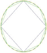
Figure 1. Polygonal approximation $\Gamma_{h,0}$ of $\Gamma(0)$ for $h=h_{0},\dots,h_{4}$.

We select the corresponding time step sizes $\tau_{0}=1$, $\tau_{j}=\tau_{j-1}/4$ and the corresponding numbers of samples $M_{1}=1$, $M_{j}=16M_{j-1}$ for $j=1,\dots,4$. The resulting discretization errors (6.2) are reported in Table 1 suggesting the optimal behavior ${\mathcal{O}}(h^{2}+M^{-1/2}+\tau)$.

$h$	$M$	$\tau$	Error	eoc($h$)	eoc($M$)	eoc($\tau$)
$1.500000$	$1$	$1$	$3.00350$	—	—	—
$0.843310$	$16$	$4^{-1}$	$2.23278\cdot 10^{-1}$	$4.51325$	$-0.93743$	$1.87487$
$0.434572$	$256$	$4^{-2}$	$1.86602\cdot 10^{-1}$	$0.27066$	$-0.06472$	$0.12944$
$0.218962$	$4\,096$	$4^{-3}$	$4.88096\cdot 10^{-2}$	$1.95642$	$-0.48368$	$0.96736$
$0.109692$	$65\,536$	$4^{-4}$	$1.29667\cdot 10^{-2}$	$1.91768$	$-0.47809$	$0.95618$

Table 1. Discretization errors for a moving curve in $\mathbb{R}^{2}$.

6.3. Moving surface

We consider the ellipsoid

$$\Gamma(t)=\left\{x=(x_{1},x_{2},x_{3})\in\mathbb{R}^{3}\;\middle|\;\frac{x_{1}^{2}}{a(t)}+x_{2}^{2}+x_{3}^{2}=1\right\},\qquad t\in[0,T],$$

with oscillating $x_{1}$-axis $a(t)=1+\tfrac{1}{4}\sin(t)$ and $T=1$. The random diffusion coefficient $\alpha$ occurring in $a_{h}(\cdot,\cdot)$ is given by

$$\alpha(x,\omega)=1+x_{1}^{2}+Y_{1}(\omega)x_{1}^{4}+Y_{2}(\omega)x_{2}^{4},$$

where $Y_{1}$ and $Y_{2}$ denote independent, uniformly distributed random variables on $\Omega=(-1,1)$. The right-hand side $f$ in (6.1) is chosen such that for each $\omega\in\Omega$ the exact solution of the resulting path-wise problem is given by

$$u(x,t,\omega)=\sin(t)x_{1}x_{2}+Y_{1}(\omega)\sin(2t)x_{1}^{2}+Y_{2}(\omega)\sin(2t)x_{2},$$

and we set $u_{0}(x,\omega)=u(x,0,\omega)=0$.

The initial triangular approximation $\Gamma_{h,0}$ of $\Gamma(0)$ is depicted in Figure 2 for the mesh sizes $h=h_{j}$, $j=0,\dots,3$.

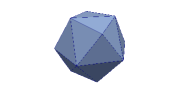
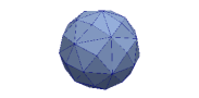
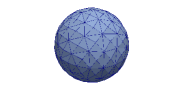
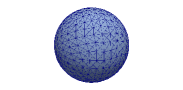
Figure 2. Triangular approximation $\Gamma_{h,0}$ of $\Gamma(0)$ for $h=h_{0},\dots,h_{3}$.

$h$	$M$	$\tau$	Error	eoc($h$)	eoc($M$)	eoc($\tau$)
$1.276870$	$1$	$1$	$9.91189\cdot 10^{-1}$	—	—	—
$0.831246$	$16$	$4^{-1}$	$1.70339\cdot 10^{-1}$	$4.10285$	$-0.63519$	$1.27037$
$0.440169$	$256$	$4^{-2}$	$4.61829\cdot 10^{-2}$	$2.05293$	$-0.47075$	$0.94149$
$0.222895$	$4\,096$	$4^{-3}$	$1.18779\cdot 10^{-2}$	$1.99561$	$-0.48977$	$0.97954$

Table 2. Discretization errors for a moving surface in $\mathbb{R}^{3}$.

We select the corresponding time step sizes $\tau_{0}=1$, $\tau_{j}=\tau_{j-1}/4$ and the corresponding numbers of samples $M_{1}=1$, $M_{j}=16M_{j-1}$ for $j=1,2,3$. The resulting discretization errors (6.2) are shown in Table 2. Again, we observe that the discretization error behaves like ${\mathcal{O}}(h^{2}+M^{-1/2}+\tau)$. This is in accordance with our theoretical findings stated in Theorem 5.5 and fully discrete deterministic results [18, Theorem 2.4].

References

- Alphonse et al. [2015a] A. Alphonse, C. M. Elliott, and B. Stinner. An abstract framework for parabolic PDEs on evolving spaces. Port. Math., 72(1):1–46, 2015a. doi: 10.4171/pm/1955.
- Alphonse et al. [2015b] A. Alphonse, C. M. Elliott, and B. Stinner. On some linear parabolic PDEs on moving hypersurfaces. Interfaces Free Bound., 17(2):157–187, 2015b. doi: 10.4171/ifb/338.
- Barth et al. [2011] A. Barth, Ch. Schwab, and N. Zollinger. Multi-level Monte Carlo finite element method for elliptic pde’s with stochastic coefficients. Numer. Math., 119(1):123–161, 2011. doi: 10.1007/s00211-011-0377-0.
- Bastian et al. [2008a] P. Bastian, M. Blatt, A. Dedner, C. Engwer, R. Klöfkorn, M. Oldberger, and O. Sander. A generic grid interface for parallel and adaptive scientific computing. Part I: Abstract framework. Computing, 82:103–119, 2008a.
- Bastian et al. [2008b] P. Bastian, M. Blatt, A. Dedner, C. Engwer, R. Klöfkorn, M. Oldberger, and O. Sander. A generic grid interface for parallel and adaptive scientific computing. Part II: Implementation and tests in Dune. Computing, 82:121–138, 2008b.
- Bertalmío et al. [2001] M. Bertalmío, Li-Tien Cheng, S. J. Osher, and G. Sapiro. Variational problems and partial differential equations on implicit surfaces. J. Comput. Phys., 174(2):759–780, 2001. ISSN 0021-9991.
- Charrier [2012] J. Charrier. Strong and weak error estimates for elliptic partial differential equations with random coefficients. SIAM J. Numer. Anal., 50(1):216–246, 2012. doi: 10.1137/100800531.
- Charrier [2015] J. Charrier. Numerical analysis of the advection-diffusion of a solute in porous media with uncertainty. SIAM/ASA J. Uncertain. Quantif., 3(1):650–685, 2015. doi: 10.1137/130937457.
- Charrier et al. [2013] J. Charrier, R. Scheichl, and A. L. Teckentrup. Finite element error analysis of elliptic pdes with random coefficients and its application to multilevel Monte Carlo methods. SIAM J. Numer. Anal., 51(1):322–352, 2013. doi: 10.1137/110853054.
- Cliffe et al. [2011] A. Cliffe, M. Giles, R. Scheichl, and A. L. Teckentrup. Multilevel Monte Carlo methods and applications to elliptic pdes with random coefficients. Comput. Vis. Sci., 14(1):3–15, 2011. doi: 10.1007/s00791-011-0160-x.
- Deckelnick et al. [2005] K. Deckelnick, G. Dziuk, and C. M. Elliott. Computation of geometric partial differential equations and mean curvature flow. Acta Numer., 14:139–232, 2005. doi: 10.1017/s0962492904000224.
- Dedner. et al. [2010] A. Dedner., R. Klöfkorn, M. Nolte, and M. Ohlberger. A generic interface for parallel and adaptive discretization schemes: abstraction principles and the Dune-Fem module. Computing, 90(3-4):165–196, 2010. doi: 10.1007/s00607-010-0110-3.
- Demlow [2009] A. Demlow. Higher-order finite element methods and pointwise error estimates for elliptic problems on surfaces. SIAM J. Numer. Anal., 47(2):805–827, 2009. doi: 10.1137/070708135.
- Djurdjevac [2015] A. Djurdjevac. Advection-diffusion equations with random coefficients on evolving hypersurfaces. Technical report, Freie Universität Berlin ( to appear in Interfaces and Free Boundaries), 2015.
- Dziuk [1988] G. Dziuk. Finite elements for the Beltrami operator on arbitrary surfaces. In S. Hildebrandt and R. Leis, editors, Partial differential equations and calculus of variations, volume 1357 of Lecture Notes in Mathematics, pages 142–155. Springer, Berlin, Heidelberg, 1988.
- Dziuk and Elliott [2006] G. Dziuk and C. M. Elliott. Finite elements on evolving surfaces. IMA J. Numer. Anal., 27(2):262–292, 2006. doi: 10.1093/imanum/drl023.
- Dziuk and Elliott [2012a] G. Dziuk and C. M. Elliott. -estimates for the evolving surface finite element method. Math. Comp., 82(281):1–24, 2012a. doi: 10.1090/s0025-5718-2012-02601-9.
- Dziuk and Elliott [2012b] G. Dziuk and C. M. Elliott. A fully discrete evolving surface finite element method. SIAM J. Numer. Anal., 50(5):2677–2694, 2012b. doi: 10.1137/110828642.
- Dziuk and Elliott [2013] G. Dziuk and C. M. Elliott. Finite element methods for surface PDEs. Acta Numer., 22:289–396, 2013. doi: 10.1017/s0962492913000056.
- Elliott and Ranner [2014] C. M. Elliott and T. Ranner. Evolving surface finite element method for the Cahn-Hilliard equation. Numer. Math., 129(3):483–534, 2014. doi: 10.1007/s00211-014-0644-y.
- Elliott et al. [2012] C. M. Elliott, B. Stinner, and C. Venkataraman. Modelling cell motility and chemotaxis with evolving surface finite elements. J. R. Soc. Interface, 82, 2012. doi: doi:10.1098/rsif.2012.0276.
- Hackbusch [2012] W. Hackbusch. Tensor Spaces and Numerical Tensor Calculus. Springer. Berlin, Heidelberg, 2012. doi: 10.1007/978-3-642-28027-6.
- Halmos [1976] P. R. Halmos. Measure Theory. Graduate Texts in Mathematics. Springer, 1976.
- Herrmann et al. [2016] L. Herrmann, A. Lang, and Ch. Schwab. Numerical analysis of lognormal diffusions on the sphere. arXiv:1601.02500v2, 2016.
- Hoang and Schwab [2013] V. H. Hoang and Ch. Schwab. Sparse tensor galerkin discretization of parametric and random parabolic PDEs—analytic regularity and generalized polynomial chaos approximation. SIAM J. Math. Anal., 45(5):3050–3083, 2013. doi: 10.1137/100793682.
- Jin et al. [2004] H. Jin, T. Yezzi, and J. Matas. Region-based segmentation on evolving surfaces with application to 3d reconstruction of shape and piecewise constant radiance. In Computer Vision - ECCV 2004: 8th European Conference on Computer Vision, Proceedings, Part II, pages 114–125. Springer Berlin Heidelberg, 2004. doi: 10.1007/978-3-540-24671-8˙9.
- Kornhuber and Yserentant [2008] R. Kornhuber and H. Yserentant. Multigrid methods for discrete elliptic problems on triangular surfaces. Comp. Vis. Sci., 11(4-6):251–257, 2008.
- Larsson et al. [2016] S. Larsson, C. Mollet, and M. Molteni. Quasi-optimality of Petrov-Galerkin discretizations of parabolic problems with random coefficients. arXiv:1604.06611, 2016.
- Lord et al. [2014] G. Lord, C. E. Powell, and T. Shardlow. An Introduction to Computational Stochastic PDEs. Cambridge University Press, 2014.
- Lubich and Mansour [2014] Ch. Lubich and D. Mansour. Variational discretization of wave equations on evolving surfaces. Math. Comp., 84(292):513–542, 2014. doi: 10.1090/s0025-5718-2014-02882-2.
- Maître and Knio [2010] O. P. Le Maître and O. M. Knio. Spectral Methods for Uncertainty Quantification. Springer Netherlands, 2010. doi: 10.1007/978-90-481-3520-2.
- Morrow and Mason [2001] N. R. Morrow and G. Mason. Recovery of oil by spontaneous imbibition. Current Opinion in Colloid and Interface Science, 6(4):321–337, 2001. doi: 10.1016/S1359-0294(01)00100-5.
- Nobile and Tempone [2009] F. Nobile and R. Tempone. Analysis and implementation issues for the numerical approximation of parabolic equations with random coefficients. Int. J. Numer. Meth. Engng., 80(6-7):979–1006, 2009. doi: 10.1002/nme.2656.
- Plaza et al. [2004] R.G. Plaza, F. Sánchez-Garduño, P. Padilla, R.A. Barrio, and P.K. Maini. The effect of growth and curvature on pattern formation. J. Dynamics and Differential Equations, 16:1093–1121, 2004.
- Reed and Simon [1980] M. Reed and B. Simon. Methods of modern mathematical physics. vol. 1. Functional analysis. Academic, New York, 1980.
- Reusken and Olshanskii [2016] A. Reusken and M.A. Olshanskii. Trace finite element methods for PDEs on surfaces. arXiv:1612.0005, 2016.