Kalman Filter and its Modern Extensions for the Continuous-time Nonlinear Filtering Problem

Abstract

This paper is concerned with the filtering problem in continuous-time. Three algorithmic solution approaches for this problem are reviewed: (i) the classical Kalman-Bucy filter which provides an exact solution for the linear Gaussian problem, (ii) the ensemble Kalman-Bucy filter (EnKBF) which is an approximate filter and represents an extension of the Kalman-Bucy filter to nonlinear problems, and (iii) the feedback particle filter (FPF) which represents an extension of the EnKBF and furthermore provides for an consistent solution in the general nonlinear, non-Gaussian case. The common feature of the three algorithms is the gain times error formula to implement the update step (to account for conditioning due to the observations) in the filter. In contrast to the commonly used sequential Monte Carlo methods, the EnKBF and FPF avoid the resampling of the particles in the importance sampling update step. Moreover, the feedback control structure provides for error correction potentially leading to smaller simulation variance and improved stability properties. The paper also discusses the issue of non-uniqueness of the filter update formula and formulates a novel approximation algorithm based on ideas from optimal transport and coupling of measures. Performance of this and other algorithms is illustrated for a numerical example.

1 Introduction

KBF	Kalman-Bucy Filter	Equations (3a)-(3b)
EKBF	Extended Kalman-Bucy Filter	Equations (5a)-(5b)
EnKBF	(Stochastic) Ensemble Kalman-Bucy Filter	Equation (7)
	(Deterministic) Ensemble Kalman-Bucy Filter	Equation (8)
FPF	Feedback Particle Filter	Equation (9)

Table 1: Nomenclature for the continuous-time filtering algorithms

Since the pioneering work of Kalman from the 1960s, sequential state estimation has been extended to application areas far beyond its original aims such as numerical weather prediction [1] and oil reservoir exploration (history matching) [2]. These developments have been made possible by clever combination of Monte Carlo techniques with Kalman-like techniques for assimilating observations into the underlying dynamical models. The most prominent of these algorithms are the ensemble Kalman filter (EnKF), the randomized maximum likelihood (RML) method and the unscented Kalman filter (UKF) invented independently by several research groups [3, 4, 5, 6] in the 1990s. The EnKF in particular can be viewed as a cleverly designed random dynamical system of interacting particles which is able to approximate the exact solution with a relative small number of particles. This interacting particle perspective has led to many new filter algorithms in recent years which go beyond the inherent Gaussian approximation of an EnKF during the data assimilation (update) step [7].

In this paper, we review the interacting particle perspective in the context of the continuous-time filtering problems and demonstrate its close relation to Kalman’s and Bucy’s original feedback control structure of the data assimilation step. More specifically, we highlight the feedback control structure of three classes of algorithms for approximating the posterior distribution: (i) the classical Kalman-Bucy filter which provides an exact solution for the linear Gaussian problem, (ii) the ensemble Kalman-Bucy filter (EnKBF) which is an approximate filter and represents an extension of the Kalman-Bucy filter to nonlinear problems, and (iii) the feedback particle filter (FPF) which represents an extension of the EnKBF and furthermore provides for a consistent solution of the general nonlinear, non-Gaussian problem.

A closely related goal is to provide comparison between these algorithms. A common feature of the three algorithms is the gain times error formula to implement the update step in the filter. The difference is that while the Kalman-Bucy filter is an exact algorithm, the two particle-based algorithms are approximate with error decreasing to zero as the number of particles $N$ increases to infinity. Algorithms with this property are said to be consistent.

In the class of interacting particle algorithms discussed, the FPF represents the most general solution to the nonlinear non-Gaussian filtering problem. The challenge with implementing the FPF lie in approximation of the “gain function” used in the update step. The gain function equals the Kalman gain in the linear Gaussian setting and must be numerically approximated in the general setting. One particular closed-form approximation is the constant gain approximation. In this case, the FPF is shown to reduce to the EnKBF algorithm. The EnKBF naturally extends to nonlinear dynamical systems and its discrete-time versions have become very popular in recent years with applications to, for example, atmosphere-ocean dynamics and oil reservoir exploration. In the discrete-time setting, development and application of closely related particle flow algorithms has also been a subject of recent interest, e.g., [8, 9, 10, 11, 12, 13].

The outline of the remainder of this paper is as follows: The continuous-time filtering problem and the classic Kalman-Bucy filter are summarized in Sections 2 and 3, respectively. The Kalman-Bucy filter is then put into the context of interacting particle systems in the form of the EnKBF in Section 4. Section 5 together with Appendices A and B provides a consistent definition of the FPF and a discussion of alternative approximation techniques which lead to consistent approximations to the filtering problem as the number of particles, $N$, goes to infinity. It is shown that the EnKBF can be viewed as an approximation to the FPF. Four algorithmic approaches to gain function approximation are described and their relationship discussed. The performance of the four algorithms is numerically studied and compared for an example problem in Section 6. The paper concludes with discussion of some open problems in Section 7. The nomenclature for the filtering algorithms described in this paper appears in Table 1.

2 Problem Statement

In the continuous-time setting, the model for nonlinear filtering problem is described by the nonlinear stochastic differential equations (sdes):

$$\text{Signal:}\quad\quad\,\mathrm{d}X_{t} =a(X_{t})\,\mathrm{d}t+\sigma(X_{t})\,\mathrm{d}B_{t},\quad\quad X_{0}\sim p_{0}^{*}$$ (1a)

$$\text{Observation:}\quad\quad\,\mathrm{d}Z_{t} =h(X_{t})\,\mathrm{d}t+\,\mathrm{d}W_{t}$$ (1b)

where $X_{t}\in\mathbb{R}^{d}$ is the (hidden) state at time $t$, the initial condition $X_{0}$ is sampled from a given prior density $p_{0}^{*}$, $Z_{t}\in\mathbb{R}^{m}$ is the observation or the measurement vector, and $\{B_{t}\}$, $\{W_{t}\}$ are two mutually independent Wiener processes taking values in $\mathbb{R}^{d}$ and $\mathbb{R}^{m}$. The mappings $a(\cdot):\mathbb{R}^{d}\rightarrow\mathbb{R}^{d}$, $h(\cdot):\mathbb{R}^{d}\rightarrow\mathbb{R}^{m}$ and $\sigma(\cdot):\mathbb{R}^{d}\rightarrow\mathbb{R}^{d\times d}$ are known $C^{1}$ functions. The covariance matrix of the observation noise $\{W_{t}\}$ is assumed to be positive definite. The function $h$ is a column vector whose $j$-th coordinate is denoted as $h_{j}$ (i.e., $h=(h_{1},h_{2},\ldots,h_{m})^{\rm T}$). By scaling, it is assumed without loss of generality that the covariance matrices associated with $\{B_{t}\}$, $\{W_{t}\}$ are identity matrices. Unless otherwise noted, the stochastic differential equations (sde) are expressed in Itô form. Table 2 includes a list of symbols used in the continuous-time filtering problem.

In applications, the continuous time filtering models are often expressed as:

$$\frac{\,\mathrm{d}X_{t}}{\,\mathrm{d}t} =a(X_{t})+\sigma(X_{t})\dot{B}_{t}$$ (2a)

$$Y_{t} :=\frac{\,\mathrm{d}Z_{t}}{\,\mathrm{d}t}=h(X_{t})+\dot{W}_{t}$$ (2b)

where $\dot{B}_{t}$ and $\dot{W}_{t}$ are mutually independent white noise processes (Gaussian noise) and $Y_{t}\in\mathbb{R}^{m}$ is the vector valued observation at time $t$. The sde-based model is preferred here because of its mathematical rigor. Any sde involving $Z_{t}$ is converted into an ODE involving $Y_{t}$ by formally dividing the sde by $\,\mathrm{d}t$ and replacing $\frac{\,\mathrm{d}Z_{t}}{\,\mathrm{d}t}$ by $Y_{t}$ (See also Remark 1).

Variable	Notation	Model
State	$X_{t}$	Eq. (1a)
Process noise	$B_{t}$	Wiener process
Measurement	$Z_{t}$	Eq. (1b)
Measurement noise	$W_{t}$	Wiener process

Table 2: Symbols for the continuous-time filtering problem

The objective of filtering is to estimate the posterior distribution of $X_{t}$ given the time history of observations ${\cal Z}_{t}:=\sigma(Z_{s}:0\leq s\leq t)$. The density of the posterior distribution is denoted by $p^{*}$, so that for any measurable set $A\subset\mathbb{R}^{d}$,

$$\int_{x\in A}p^{*}(x,t)\,\,\mathrm{d}x={\sf P}\{X_{t}\in A\mid{\cal Z}_{t}\}$$

One example of particular interest is when the mappings $a(x)$ and $h(x)$ are linear, $\sigma(x)$ is a constant matrix that does not depend upon $x$, and the prior density $p_{0}^{*}$ is Gaussian. The associated problem is referred to as the linear Gaussian filtering problem. For this problem, the posterior density is known to be Gaussian. The resulting filter is said to be finite-dimensional because the posterior is completely described by finitely many statistics – conditional mean and variance in the linear Gaussian case.

For the general nonlinear non-Gaussian case, however, the filter is infinite-dimensional because it defines the evolution, in the space of probability measures, of $\{p^{*}(\,\cdot\,,t):t\geq 0\}$. The particle filter is a simulation-based algorithm to approximate the posterior: The key step is the construction of $N$ interacting stochastic processes $\{X^{i}_{t}:1\leq i\leq N\}$: The value $X^{i}_{t}\in\mathbb{R}^{d}$ is the state for the $i$-th particle at time $t$. For each time $t$, the empirical distribution formed by the particle population is used to approximate the posterior distribution. Recall that this is defined for any measurable set $A\subset\mathbb{R}^{d}$ by,

$$p^{(N)}(A,t)=\frac{1}{N}\sum_{i=1}^{N}\text{\rm\large 1}\{X^{i}_{t}\in A\}\,.$$

where $\text{\rm\large 1}\{x\in A\}$ is the indicator function (equal to $1$ if $x\in A$ and $0$ otherwise). The first interacting particle representation of the continuous-time filtering problem can be found in [14, 15]. The close connection of such interacting particle formulations to the gain factor and innovation structure of the classic Kalman filter has been made explicit starting with [16, 17] and has led to the FPF formulation considered in this paper.

Notation: The density for a Gaussian random variable with mean $m$ and variance $\Sigma$ is denoted as ${\cal N}(m,\Sigma)$. For vectors $x,y\in\mathbb{R}^{d}$, the dot product is denoted as $x\cdot y$ and $|x|:=\sqrt{x\cdot x}$; $x^{\rm T}$ denotes the transpose of the vector. Similarly, for a matrix ${\sf K}$, ${\sf K}^{\rm T}$ denotes the matrix transpose. For two sequence $\{a_{n}\}_{n=1}^{\infty}$ and $\{b_{n}\}_{n=1}^{\infty}$, the big $O$ notation $a_{n}=O(b_{n})$ means $\exists\,n_{0}\in\mathbb{N}$ and $c>0$ such that $|a_{n}|\leq c|b_{n}|$ for $n>n_{0}$.

3 Kalman-Bucy Filter

Variable	Notn. & Defn.	Model
Cond. mean	$\hat{X}_{t}={\sf E}[X_{t}|{\cal Z}_{t}]$	Eq. (3a)
Cond. var.	$\Sigma_{t}={\sf E}[(X_{t}-\hat{X}_{t})(X_{t}-\hat{X}_{t})^{T}|{\cal Z}_{t}]$	Eq. (3b)
Kalman gain	${\sf K}_{t}=\Sigma_{t}H_{t}^{T}$	Eq. (4)

Table 3: Symbols for the Kalman filter

Consider the linear Gaussian problem: The mappings $a(x)=A\,x$ and $h(x)=H\,x$ where $A$ and $H$ are $d\times d$ and $m\times d$ matrices; the process noise covariance $\sigma(x)=\sigma$, a constant $d\times d$ matrix; and the prior density is Gaussian, denoted as ${\cal N}(\hat{X}_{0},\Sigma_{0})$.

For this problem, the posterior density is known to be Gaussian, denoted as ${\cal N}(\hat{X}_{t},\Sigma_{t})$, where $\hat{X}_{t}$ and $\Sigma_{t}$ are the conditional mean and variance, i.e $\hat{X}_{t}:={\sf E}[X_{t}|{\cal Z}_{t}]$ and $\Sigma_{t}:={\sf E}[(X_{t}-\hat{X}_{t})(X_{t}-\hat{X}_{t})^{T}|{\cal Z}_{t}]$. Their evolution is described by the finite-dimensional Kalman-Bucy filter:

$$\,\mathrm{d}\hat{X}_{t} =A\hat{X}_{t}\,\mathrm{d}t+{\sf K}_{t}\Bigl{(}\,\mathrm{d}Z_{t}-H_{t}\hat{X}_{t}\,\mathrm{d}t\Bigr{)}$$ (3a)

$$\frac{\,\mathrm{d}\Sigma_{t}}{\,\mathrm{d}t} =A\Sigma_{t}+\Sigma_{t}A^{T}+\sigma\sigma^{T}-\Sigma_{t}H^{T}H\Sigma_{t}$$ (3b)

where

$${\sf K}_{t}:=\Sigma_{t}H_{t}^{\rm T}$$ (4)

is referred to as the Kalman gain and the filter is initialized with the initial conditions $\hat{X}_{0}$ and $\Sigma_{0}$ of the prior density. Table 3 includes a list of symbols used for the Kalman filter.

The evolution equation for the mean is a sde because of the presence of stochastic forcing term $Z_{t}$ on the right-hand side. The evolution equation for the variance $\Sigma_{t}$ is an ode that does not depend upon the observation process.

The Kalman filter is one of the most widely used algorithm in engineering. Although the filter describes the posterior only in linear Gaussian settings, it is often used as an approximate algorithm even in more general settings, e.g., by defining the matrices $A$ and $H$ according to the Jacobians of the mappings $a$ and $h$:

$$A:=\frac{\partial a}{\partial x}(\hat{X}_{t}),\quad H:=\frac{\partial h}{\partial x}(\hat{X}_{t})$$

The resulting algorithm is referred to as the extended Kalman filter:

$$\,\mathrm{d}\hat{X}_{t} =a(\hat{X}_{t})\,\mathrm{d}t+{\sf K}_{t}\Bigl{(}\,\mathrm{d}Z_{t}-h(\hat{X}_{t})\,\mathrm{d}t\Bigr{)}$$ (5a)

$$\frac{\,\mathrm{d}\Sigma_{t}}{\,\mathrm{d}t} =A\Sigma_{t}+\Sigma_{t}A^{T}+\sigma(\hat{X}_{t})\sigma^{T}(\hat{X}_{t})-\Sigma_{t}H^{T}H\Sigma_{t}$$ (5b)

where ${\sf K}_{t}=\Sigma_{t}H^{\rm T}$ is used as the formula for the gain.

The Kalman filter and its extensions are recursive algorithms that process measurements in a sequential (online) fashion. At each time $t$, the filter computes an error $\,\mathrm{d}Z_{t}-H\hat{X}_{t}\,\mathrm{d}t$ (called the innovation error) which reflects the new information contained in the most recent measurement. The filter state $\hat{X}_{t}$ is corrected at each time step via a $(\text{gain}\times\text{error})$ update formula.

The error correction feedback structure (see Fig. 1) is important on account of robustness. A filter is based on an idealized model of an underlying stochastic dynamic process. The self-correcting property of the feedback provides robustness, allowing one to tolerate a degree of uncertainty inherent in any model.

The simple intuitive nature of the update formula is invaluable in design, testing and operation of the filter. For example, the Kalman gain is proportional to $H$ which scales with the signal-to-noise ratio of the measurement model. In practice, the gain may be ‘tuned’ to optimize the filter performance. To minimize online computations, an offline solution of the algebraic Ricatti equation (obtained after equating the right-hand side of the variance ode (3b) to zero) may be used to obtain a constant value for the gain.

The basic Kalman filter has also been extended to handle filtering problems involving additional uncertainties in the signal model and the observation model. The resulting (approximate) algorithms are referred to as the interacting multiple model (IMM) filter [18] and the probabilistic data association (PDA) filter [19], respectively. In the PDA filter, the gain varies based on an estimate of the instantaneous uncertainty in the measurements. In the IMM filter, multiple Kalman filters are run in parallel and their outputs combined to obtain an estimate.

One explanation of the feedback control structure of the Kalman filter is based on duality between estimation and control [20]. Although limited to linear Gaussian problems, these considerations also help explain the differential Ricatti equation structure for the variance ode (3b).

Although widely used, the extended Kalman filter can suffer from stability issues because of the very crude approximation of the nonlinear model. The observed divergence arises on account of two inter-related reasons: (i) Even with Gaussian process and measurement noise, the nonlinearity of the mappings $a(\cdot)$, $\sigma(\cdot)$ and $h(\cdot)$ can lead to non-Gaussian forms of the posterior density $p^{*}$; and (ii) the Jacobians $A$ and $H$ used in propagating the covariance can lead to large errors in approximation of the gain particularly if the Hessian of these mappings is large. These issues have necessitated development of particle based algorithms described in the following sections.

Variable	Notation	Model
Particle state	$X^{i}_{t}$	Stoch. EnKBF Eq. (7)
		Deter. EnKBF Eq. (8)
Empirical variance	$\Sigma_{t}^{(N)}$	Eq. (6)
Particle process noise	$B^{i}_{t}$	Wiener process
Particle meas. noise	$W^{i}_{t}$	Wiener process

Table 4: Symbols for the ensemble Kalman-Bucy filter

4 Ensemble Kalman-Bucy Filter

For pedagogical reasons, the ensemble Kalman-Bucy filter (EnKBF) is best described for the linear Gaussian problem – also the approach taken in this section. The extension to the nonlinear non-Gaussian problem is then immediate, similar to the extension from the Kalman filter to the extended Kalman filter.

Even in linear Gaussian settings, a particle filter may be a computationally efficient option for problems with very large state dimension $d$ (e.g., weather models in meteorology). For large $d$, the computational bottleneck in simulating a Kalman filter arises due to propagation of the covariance matrix according to the differential Riccati equation (3b). This computation scales as $O(d^{2})$ in memory. In an EnKBF implementation, one replaces the exact propagation of the covariance matrix by an empirical approximation with $N$ particles

$$\qquad\Sigma_{t}^{(N)} =\frac{1}{N-1}\sum_{i=1}^{N}(X_{t}^{i}-\hat{X}_{t}^{(N)})(X_{t}^{i}-\hat{X}_{t}^{(N)})^{\rm T}$$ (6)

This computation scales as $O(Nd)$. The same reduction in computational cost can be achieved by a reduced rank Kalman filter. However, the connection to empirical measures (2) is crucial to the application of the EnKBF to nonlinear dynamical systems.

The EnKF algorithm was first developed in a discrete-time setting [4]. Since then various formulations of the EnKF have been proposed [21, 7]. Below we state two continuous-time formulations of the EnKBF. Table 4 includes a list of symbols used for these formulations.

4.1 Stochastic EnKBF

The conceptual idea of the stochastic EnKBF algorithm is to introduce a zero mean perturbation (noise term) in the innovation error to achieve consistency for the variance update. In the continuous-time stochastic EnKBF algorithm, the particles evolve according to

$$\,\mathrm{d}X_{t}^{i}=AX_{t}^{i}\,\mathrm{d}t+\sigma\,\mathrm{d}B_{t}^{i}+\Sigma^{(N)}_{t}H^{{\rm T}}\Big{(}\,\mathrm{d}{Z}_{t}^{i}-HX^{i}_{t}\,\mathrm{d}t+\,\mathrm{d}W_{t}^{i}\Big{)}$$ (7)

for $i=1,\ldots,N$, where $X_{t}^{i}\in\mathbb{R}^{d}$ is the state of the $i^{\text{th}}$ particle at time $t$, the initial condition $X^{i}_{0}\sim p_{0}^{*}$, $B^{i}_{t}$ is a standard Wiener process, and $W_{t}^{i}$ is a standard Wiener process assumed to be independent of $X_{0}^{i},\,B_{t}^{i},\,X_{t},\,Z_{t}$  [21]. The variance $\Sigma^{(N)}_{t}$ is obtained empirically using (6). Note that the $N$ particles only interact through the common covariance matrix $\Sigma_{t}^{(N)}$.

The idea of introducing a noise process first appeared for the discrete-time EnKF. The derivation of the continuous-time stochastic EnKBF can be found in [21] or [22]. It is based on a limiting argument whereby the discrete-time update step is formally viewed as an Euler-Maruyama discretization of a stochastic SDE. For the linear Gaussian problem, the stochastic EnKBF algorithm is consistent in the limit as $N\rightarrow\infty$. This means that the conditional distribution of $X_{t}^{i}$ is Gaussian whose mean and variance evolve according the Kalman filter, equations (3a) and (3b), respectively.

The update formula used in (7) is not unique. A deterministic analogue is described next.

4.2 Deterministic EnKBF

A deterministic variant of the EnKBF (first proposed in [23]) is given by:

$$\,\mathrm{d}X_{t}^{i}=AX_{t}^{i}\,\mathrm{d}t+\sigma\,\mathrm{d}B_{t}^{i}+\Sigma_{t}^{(N)}H^{\rm T}\left(\,\mathrm{d}Z_{t}-\frac{HX_{t}^{i}+H\hat{X}_{t}^{(N)}}{2}{\rm d}t\right)$$ (8)

for $i=1,\ldots,N$. A proof of the consistency of this deterministic variant of the EnKBF for linear systems can be found in [24]. There are close parallels between the deterministic EnKBF and the FPF which is explored further in Section 5. In the deterministic formulation of the EnKBF the interaction between the $N$ particles arises through the covariance matrix $\Sigma^{(N)}_{t}$ and the mean $\hat{X}_{t}^{(N)}$.

Although the stochastic and the deterministic EnKBF algorithms are consistent for the linear Gaussian problem, they can be easily extended to the nonlinear non-Gaussian settings. However, the resulting algorithm will in general not be consistent.

4.3 Well-posedness and accuracy of the EnKBF

Recent research on EnKF has focussed on the long term behavior and accuracy of filters applicable for nonlinear data assimilation [25, 24, 26, 27]. In particular the mathematical justification for the feasibility of the EnKF and its continuous counterpart in the small ensemble limit are of interest. These studies of the accuracy for a finite ensemble are of exceptional importance due to the fact that a large number of ensemble members is not an option from a computational point of view in many applicational areas. The authors of [26] show mean-squared asymptotic accuracy in the large-time limit where a particular type of variance inflation is deployed for the stochastic EnKBF. Well-posedness of the discrete and continuous formulation of the EnKF is also shown. Similar results concerning the well-posedness and accuracy for the deterministic variant (8) of the EnKBF are derived in [24]. A fully observed system is assumed in deriving these accuracy and well-posedness results. An investigation of the well-posedness for partially observed systems is particularly relevant as the update step in such cases can cause a divergence of the estimate in the sense that the signal is lost or the values of the estimate reach machine infinity [28].

5 Feedback Particle Filter

The FPF is a controlled sde:

$$\,\mathrm{d}X^{i}_{t}= a(X^{i}_{t})\,\mathrm{d}t+\sigma(X_{t}^{i})\,\mathrm{d}B^{i}_{t}$$ (9)

$$+\underbrace{{\sf K}_{t}(X^{i}_{t})\circ(\,\mathrm{d}Z_{t}-\frac{h(X^{i}_{t})+\hat{h}_{t}}{2}\,\mathrm{d}t)}_{\text{update}},\quad X_{0}^{i}\sim p_{0}^{*}$$

where (similar to EnKBF) $X_{t}^{i}\in\mathbb{R}^{d}$ is the state of the $i^{\text{th}}$ particle at time $t$, the initial condition $X^{i}_{0}\sim p_{0}^{*}$, $B^{i}_{t}$ is a standard Wiener process, and $\hat{h}_{t}:={\sf E}[h(X_{t}^{i})|\mathcal{Z}_{t}]$. Both $B^{i}_{t}$ and $X^{i}_{0}$ are mutually independent and also independent of $X_{t},Z_{t}$. The $\circ$ in the update term indicates that the sde is expressed in its Stratonovich form.

The gain function ${\sf K}_{t}$ is vector-valued (with dimension $d\times m$) and it needs to be obtained for each fixed time $t$. The gain function is defined as a solution of a pde introduced in the following subsection. For the linear Gaussian problem, ${\sf K}_{t}$ is the Kalman gain. For the general nonlinear non-Gaussian, the gain function needs to be numerically approximated. Algorithms for this are also summarized in the following subsection.

Remark 1

Given that the Stratonovich form provides a mathematical interpretation of the (formal) ode model [29, see Section 3.3 of the sde textbook by Øksendal], we also obtain the (formal) ode model of the filter. Denoting $Y_{t}\doteq\frac{\,\mathrm{d}Z_{t}}{\,\mathrm{d}t}$ and white noise process $\dot{B}^{i}_{t}\doteq\frac{\,\mathrm{d}B_{t}^{i}}{\,\mathrm{d}t}$, the ODE model of the filter is given by,

$$\frac{\,\mathrm{d}X^{i}_{t}}{\,\mathrm{d}t}=a(X^{i}_{t})+\sigma(X_{t}^{i})\dot{B}^{i}_{t}+{\sf K}(X^{i},t)\left(Y_{t}-\frac{1}{2}(h(X^{i}_{t})+\hat{h})\right),$$

for $i=1,\ldots,N$. The feedback particle filter thus provides a generalization of the Kalman filter to nonlinear systems, where the innovation error-based feedback structure of the control is preserved (see Fig. 1). For the linear Gaussian case, the gain function is the Kalman gain. For the nonlinear case, the Kalman gain is replaced by a nonlinear function of the state (See Fig. 3).

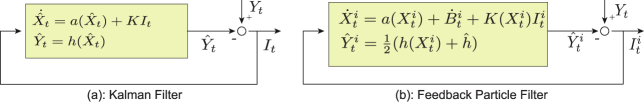
Figure 1: Innovation error-based feedback structure for the (a) Kalman filter and (b) nonlinear feedback particle filter.

Remark 2

It is shown in Appendix A that, under the condition that the gain function can be computed exactly, FPF is an exact algorithm. That is, if the initial condition $X^{i}_{0}$ is sampled from the prior $p_{0}^{*}$ then

$${\sf P}[X_{t}\in A\mid{\cal Z}_{t}]={\sf P}[X_{t}^{i}\in A\mid{\cal Z}_{t}],\quad\forall\;A\subset\mathbb{R}^{d},\;\;t>0.$$

In a numerical implementation, a finite number, $N$, of particles is simulated and ${\sf P}[X_{t}^{i}\in A\mid{\cal Z}_{t}]\approx\frac{1}{N}\sum_{i=1}^{N}\text{\rm\large 1}[X^{i}_{t}\in A]$ by the Law of Large Numbers (LLN).

The considerations in the Appendix are described in a more general setting, e.g., applicable to stochastic processes $X_{t}$ and $X_{t}^{i}$ evolving on manifolds. This also explains why the update formula has a Stratonovich form. For sdes on a manifold, it is well known that the Stratonovich form is invariant to coordinate transformations (i.e., intrinsic) while the Ito form is not. A more in-depth discussion of the FPF for Lie groups appears in [30].

Table 5 includes a list of symbols used for the FPF.

Variable	Notation	Model
Particle state	$X^{i}_{t}$	FPF Eq. (9)
Gain function	${\sf K}_{t}(x)=\nabla\phi(x)$	Poisson Eq. (10)
Particle gain	${\sf K}^{i}={\sf K}(X^{i}_{t})$	Constant gain (14)
		Galerkin (17)
		Kernel-based (22)
		Optimal coupling (25)

Table 5: Symbols for feedback particle filter

5.1 Gain function

For pedagogical reasons primarily to do with notational convenience, the gain function is defined here for the case of scalar-valued observation. In this case, the gain function ${\sf K}_{t}$ is defined in terms of the solution of the weighted Poisson equation:

$$-\nabla\cdot(\rho(x)\nabla\phi(x)) =(h(x)-\hat{h})\rho(x),\quad x\in\mathbb{R}^{d}$$ (10)

$$\int\phi(x)\rho(x)\,\mathrm{d}x =0$$

where $\hat{h}:=\int h(x)\rho(x)\,\mathrm{d}x$, $\nabla$ and $\nabla\cdot$ denote the gradient and the divergence operators, respectively, and at time $t$, $\rho(x)=p(x,t)$ denotes the density of $X_{t}^{i}$. In terms of the solution $\phi(x)$ of (10), the gain function at time $t$ is given by

$${\sf K}_{t}(x)=\nabla\phi(x)\,.$$ (11)

Remark 3

The gain function ${\sf K}_{t}(x)$ is not uniquely defined through the filtering problem. Formula (11) represents one choice of the gain function. More generally, it is sufficient to require that ${\sf K}_{t}={\sf K}$ is a solution of

$$-\nabla\cdot(\rho(x){\sf K}(x))=(h(x)-\hat{h})\rho(x),\quad x\in\mathbb{R}^{d}$$ (12)

with $\rho(x)=p(x,t)$ at time $t$.

One justification for choosing the gradient form solution, as in (11), is its $L^{2}$ optimality. The general solution of (12) is given by

$${\sf K}=\nabla\phi+v$$

where $\phi$ is the solution of (10) and $v$ solves $\nabla\cdot(\rho v)=0$. It is easy to see that

$${\sf E}[|{\sf K}|^{2}]={\sf E}[|\nabla\phi|^{2}]+{\sf E}[|v|^{2}].$$

Therefore, ${\sf K}=\nabla\phi$ is the minimum $L^{2}$-norm solution of (12). By interpreting the $L^{2}$ norm as the kinetic energy, the gain function ${\sf K}_{t}=\nabla\phi$, defined through (10), is seen to be optimal in the sense of optimal transportation [32, 33].

An alternative solution of (12) is provided through the definition

$${\sf K}_{t}(x)=\frac{1}{\rho(x)}\nabla\tilde{\phi}(x)$$

which leads to a standard Poisson equation in the unknown potential $\tilde{\phi}$ for which the fundamental solution is explicitly known. This fact is exploited in the interacting particle filter representations of [14, 15].

There are two special cases of (10) – summarized as part of the following two examples – where the exact solution can be found.

Example 1

In the scalar case (where $d=1$), the Poisson equation is:

$$-\frac{1}{\rho(x)}\frac{\,\mathrm{d}}{\,\mathrm{d}x}(\rho(x)\frac{\,\mathrm{d}\phi}{\,\mathrm{d}x}(x))=h-\hat{h}.$$

Integrating once yields the solution explicitly,

$${\sf K}(x)=\frac{\,\mathrm{d}\phi}{\,\mathrm{d}x}(x) =-\frac{1}{\rho(x)}\int_{-\infty}^{x}\rho(z)(h(z)-\hat{h})\,\mathrm{d}z.$$ (13)

For the particular choice of $\rho$ as the sum of two Gaussians ${\cal N}(-1,\sigma^{2})$ and ${\cal N}(+1,\sigma^{2})$ with $\sigma^{2}=0.2$ and $h(x)=x$, the solution obtained using (13) is depicted in Fig. 2.

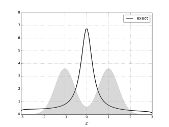
Figure 2: The exact solution to the Poisson equation using the formula (13). The density $\rho$ is the sum of two Gaussians $N(-1,\sigma^{2})$ and $N(+1,\sigma^{2})$, and $h(x)=x$. The density is depicted as the shaded curve in the background.

Example 2

Suppose the density $\rho$ is a Gaussian ${\cal N}(\mu,\Sigma)$. The observation function $h(x)=Hx$, where $H\in\mathbb{R}^{1\times d}$. Then, $\phi=x^{\rm T}\Sigma H^{\rm T}$ and the gain function ${\sf K}=\Sigma\,H^{\rm T}$ is the Kalman gain.

In the general non-Gaussian case, the solution is not known in an explicit form and must be numerically approximated. Note that even in the two exact cases, one would need to numerically approximate the solution because the density $\rho$ is not available in an explicit form.

The problem statement for numerical approximation is as follows:

Problem statement: Given $N$ samples $\{X^{1},\ldots,X^{i},\ldots,X^{N}\}$ drawn i.i.d. from $\rho$, approximate the vector-valued gain function$\{{\sf K}^{1},\ldots,{\sf K}^{i},\ldots,{\sf K}^{N}\}$, where ${\sf K}^{i}:={\sf K}(X^{i})=\nabla\phi(X^{i})$. The density $\rho$ is not explicitly known.

Four numerical algorithms for approximation of the gain function appear in the following four subsections.

5.2 Constant Gain Approximation

The constant gain approximation is the best – in the least-square sense – constant approximation of the gain function (see Figure 3). Mathematically, it is obtained by considering the following least-square optimization problem:

$$\kappa^{\ast}=\arg\min_{\kappa\in\mathbb{R}^{d}}{\sf E}\,[|{\sf K}-\kappa|^{2}]$$

By using a standard sum of the squares argument, $\kappa^{\ast}={\sf E}[{\sf K}].$ By multiplying both sides of the pde (10) by $x$ and integrating by parts, the expected value is computed explicitly as

$$\kappa^{*}={\sf E}[{\sf K}] =\int_{\mathbb{R}^{d}}(h(x)-\hat{h})\;x\;\rho(x)\,\mathrm{d}x$$

The integral is evaluated empirically to obtain the following approximate formula for the gain:

$${\sf K}^{i}\equiv\frac{1}{N}\sum_{j=1}^{N}\;(h(X^{j})-\hat{h}^{(N)})\;X^{j}$$ (14)

where $\hat{h}^{(N)}=N^{-1}\sum_{j=1}^{N}h(X^{j})$. The formula (14) is referred to as the constant gain approximation of the gain function; cf., [31]. It is a popular choice in applications [31, 35, 36, 37] and is equivalent to the approximation used in the deterministic and stochastic EnKBF [7, 21, 22, 23, 24].

Example 3

Consider the linear case where $h(x)=Hx$. The constant gain approximation formula equals

$${\sf K}^{i}=\frac{1}{N}\sum_{j=1}^{N}\;(HX^{j}-H\hat{X}^{(N)})\;X^{i}=\Sigma^{(N)}H,$$

where $\hat{X}^{(N)}:=\frac{1}{N}\sum_{i=1}^{N}X^{i}$ and $\Sigma^{N}=\frac{1}{N}\sum_{i=1}^{N}(X^{i}-\hat{X}^{(N)})(X^{i}-\hat{X}^{(N)})^{\rm T}$ are the empirical mean and the empirical variance, respectively. That is, for the linear Gaussian case, the FPF algorithm with the constant gain approximation gives the deterministic EnKF algorithm.

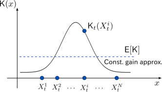
Figure 3: Constant gain approximation in the feedback particle filter

5.3 Galerkin Approximation

The Galerkin approximation is a generalization of the constant gain approximation where the gain function ${\sf K}=\nabla\phi$ is now approximated in a finite-dimensional subspace $S:=\text{span}\{\psi_{1},\ldots,\psi_{M}\}$. Mathematically, the Galerkin solution $\nabla\phi^{(M)}$ is defined as the optimal least-square approximation of $\nabla\phi$ in $S$, i.e,

$$\phi^{(M)}=\mathop{\text{\rm arg\,min}}_{\psi\in S}~{}{\sf E}[|\nabla\phi-\nabla\psi|^{2}]$$

The least-square solution is easily obtained by applying the projection theorem which gives

$${\sf E}[\nabla\phi^{(M)}\cdot\nabla\psi]={\sf E}[(h-\hat{h})\,\psi],\quad\forall\;\psi\in S$$ (15)

By denoting $(\psi_{1}(x),\psi_{2}(x),\ldots,\psi_{M}(x))=:\psi(x)$ and expressing $\phi^{(M)}(x)=c\cdot\psi(x)$, the finite dimensional system (15) is expressed as a linear matrix equation

$$Ac=b$$ (16)

where $A$ is a $M\times M$ matrix and $b$ is a $M\times 1$ vector whose entries are given by the respective formulae:

$$[A]_{lk} ={\sf E}[\nabla\psi_{l}\cdot\nabla\psi_{k}]$$

$$[b]_{l} ={\sf E}[(h-\hat{h})\,\psi_{l}]$$

Example 4

Two types of approximations follow from consideration of two types of basis functions:

• The constant gain approximation is obtained by taking basis functions as $\psi_{l}(x)=x_{l}$ for $l=1,\ldots,d$. With this choice, $A$ is the identity matrix and the Galerkin gain function is a constant vector:

  $${\sf K}(x)=\int x\,(h(x)-\hat{h})\,\rho(x)\,\mathrm{d}x$$

  It’s empirical approximation is

  $${\sf K}^{i}\equiv\frac{1}{N}\sum_{j=1}^{N}\;(h(X^{j})-\hat{h}^{(N)})\;X^{j}$$

• With a single basis function $\psi(x)=h(x)$, the Galerkin solution is

  $${\sf K}(x)=\frac{\int(h(x)-\hat{h})^{2}\rho(x)\,\mathrm{d}x}{\int|\nabla h(x)|^{2}\rho(x)\,\mathrm{d}x}\;\nabla h(x)$$

  It’s empirical approximation is obtained as

  $${\sf K}^{i}=\frac{\sum_{j=1}^{N}(h(X_{t}^{i})-\hat{h}^{(N)})^{2}}{\sum_{j=1}^{N}|\nabla h(X_{t}^{i})|^{2}}\;\nabla h(X_{t}^{i})$$

Algorithm 1 Constant gain approximation

0:  $\{X^{i}\}_{i=1}^{N}$, $\{h(X^{i})\}_{i=1}^{N}$,

0:  $\{{\sf K}^{i}\}_{i=1}^{N}$,

1:  Calculate $\hat{h}^{(N)}=\frac{1}{N}\sum_{i=1}^{N}h(X^{i})$

2:  Calculate ${\sf K}_{c}=\frac{1}{N}\sum_{i=1}^{N}\;(h(X^{i})-\hat{h}^{(N)})\;X^{i}$

3:  $K^{i}={\sf K}_{c}$ for $i=1,\ldots,N$

Algorithm 2 Galerkin approximation of the gain function

0:  $\{X^{i}\}_{i=1}^{N}$, $\{h(X^{i})\}_{i=1}^{N}$, $\{\psi_{1},\ldots,\psi_{M}\}$,

0:  $\{{\sf K}^{i}\}_{i=1}^{N}$,

1:  $\hat{h}^{(N)}=\frac{1}{N}\sum_{i=1}^{N}h(X^{i})$

2:  $[A^{(N)}]_{lk}:=\frac{1}{N}\sum_{i=1}^{N}\nabla\psi_{l}(X^{i})\cdot\nabla\psi_{k}(X^{i}),$ for $l,k=1,\ldots,M$

3:  $[b^{(N)}]_{k}:=\frac{1}{N}\sum_{i=1}^{N}\psi_{k}(X^{i})(h(X^{i})-\hat{h}^{(N)})$, for $k=1,\ldots,M$

4:  Calculate $c^{(N)}$ by solving $A^{(N)}c^{(N)}=b^{(N)}$

5:  ${\sf K}^{i}=\sum_{k=1}^{M}c^{(N)}_{k}\nabla\psi_{k}(X^{i})$

In practice, the matrix $A$ and the vector $b$ are approximated empirically, and the equation (16) solved to obtain the empirical approximation of $c$, denoted as $c^{(N)}$ (see Table 2 for the Galerkin algorithm). In terms of this empirical approximation, the gain function is approximated as

$${\sf K}^{i}=\nabla\phi^{(M,N)}(X^{i}):=c^{(N)}\cdot\nabla\psi(X^{i})$$ (17)

The choice of basis function is problem dependent. In Euclidean settings, the linear basis functions are standard and lead to constant gain approximation as discussed in Example 4. A straightforward extension is to choose quadratic and higher order polynomials as basis functions. However, this approach does not scale well with the dimension of problem: The number of basis functions $M$ scales at least linearly with dimension, and the Galerkin algorithm involves inverting a $M\times M$ matrix. This motivates nonparametric and data driven approaches where (a small number of) basis functions can be selected in an adaptive fashion. One such algorithm, proposed in [38], is based on the Karhunen-Loeve expansion.

In the next two subsections, alternate data-driven algorithms are described. One advantage of these algorithms is that they do not require a selection of basis functions.

5.4 Kernel-based Approximation

The linear operator $\frac{1}{\rho}\nabla\cdot(\rho\nabla)=:\Delta_{\rho}$ for the pde (10) is a generator of a Markov semigroup, denoted as $e^{\epsilon\Delta_{\rho}}$ for $\epsilon>0$. It follows that the solution $\phi$ of (10) is equivalently expressed as, for any fixed $\epsilon>0$,

$$\phi=e^{\epsilon\Delta_{\rho}}\phi+\int_{0}^{\epsilon}e^{s\Delta_{\rho}}(h-\hat{h})\,\mathrm{d}s.$$ (18)

The fixed-point representation is useful because $e^{\epsilon\Delta_{\rho}}$ can be approximated by a finite-rank operator

$${T}^{(N)}_{\epsilon}f(x):=\sum_{i=1}^{N}{k}_{\epsilon}^{(N)}(x,X^{i})f(X^{i}),$$

where the kernel

$${k}_{\epsilon}^{(N)}(x,y)=\frac{1}{{n}_{\epsilon}^{(N)}(x)}\frac{{g}_{\epsilon}(x-y)}{\sqrt{\frac{1}{N}\sum_{i=1}^{N}{g}_{\epsilon}(x-X^{i})}\sqrt{\frac{1}{N}\sum_{i=1}^{N}{g}_{\epsilon}(y-X^{i})}}$$

is expressed in terms of the Gaussian kernel ${g}_{\epsilon}(z):={(4\pi\epsilon)}^{-\frac{d}{2}}\exp{(-\frac{|z|^{2}}{4\epsilon})}$ for $z\in\mathbb{R}^{d}$, and ${n}_{\epsilon}^{(N)}(x)$ is a normalization factor chosen such that ${T}^{(N)}_{\epsilon}1=1$. It is shown in [39, 40] that $e^{\epsilon\Delta\rho}\approx{T}^{(N)}_{\epsilon}$ as $\epsilon\downarrow 0$ and $N\to\infty$.

The approximation of the fixed-point problem (18) is obtained as

$${\phi}^{(N)}_{\epsilon}={T}^{(N)}_{\epsilon}{\phi}^{(N)}_{\epsilon}+\epsilon(h-\hat{h}),$$ (19)

where $\int_{0}^{\epsilon}e^{s\Delta_{\rho}}(h-\hat{h})\,\mathrm{d}s\approx\epsilon(h-\hat{h})$ for small $\epsilon>0$. The method of successive approximation is used to solve the fixed-point equation for ${\phi}^{(N)}_{\epsilon}$. In a recursive simulation, the algorithm is initialized with the solution from the previous time-step.

The gain function is obtained by taking the gradient of the two sides of (19). For this purpose, it is useful to first define a finite-rank operator:

$$\nabla {T}^{(N)}_{\epsilon}f(x):=\sum_{i=1}^{N}\nabla{k}_{\epsilon}^{(N)}(x,X^{i})f(X^{i})$$ (20)

$$=\frac{1}{2\epsilon}\left[\sum_{i=1}^{N}{k}_{\epsilon}^{(N)}(x,X^{i})f(X^{i})\left(X^{i}-\sum_{j=1}^{N}{k}_{\epsilon}^{(N)}(x,X^{j})X^{j}\right)\right]$$

In terms of this operator, the gain function is approximated as

$${\sf K}^{i}=\nabla{T}^{(N)}_{\epsilon}{\phi}^{(N)}_{\epsilon}(X^{i})+\epsilon\nabla{T}^{(N)}_{\epsilon}(h-\hat{h}^{(N)})(X^{i})$$ (21)

where ${\phi}^{(N)}_{\epsilon}$ on the righthand-side is the solution of (19).

For $i,j\in\{1,2,\ldots,N\}$, denote

$$a_{ij}:=\frac{1}{2\epsilon}{k}_{\epsilon}^{(N)}(X^{i},X^{j})\left(r_{j}-\sum_{l=1}^{N}{k}_{\epsilon}^{(N)}(X^{i},X^{l})r_{l}\right)$$

where $r_{i}:={\phi}^{(N)}_{\epsilon}(X^{i})+\epsilon h(X^{i})-\epsilon\hat{h}^{(N)}$. Then, the formula (21) is succinctly expressed as

$${\sf K}^{i}=\sum_{j=1}^{N}a_{ij}X^{j}$$ (22)

It is easy to verify that $\sum_{j=1}^{N}a_{ij}=0$ and as $\epsilon\rightarrow\infty$, $a_{ij}={N}^{-1}(h(X^{j})-\hat{h}^{(N)})$. Therefore, as $\epsilon\rightarrow\infty$, ${\sf K}^{i}$ equals the constant gain approximation formula (14).

Algorithm 3 Kernel-based approximation of the gain function

0:  $\{X^{i}\}_{i=1}^{N}$, $\{h(X^{i})\}_{i=1}^{N}$, $\Phi_{\text{prev}}$, $L$

0:  $\{{\sf K}^{i}\}_{i=1}^{N}$

1:  Calculate $g_{ij}:=\exp(-|X^{i}-X^{j}|^{2}/4\epsilon)$ for $i,j=1$ to $N$

2:  Calculate $k_{ij}:=\frac{g_{ij}}{\sqrt{\sum_{l}g_{il}}\sqrt{\sum_{l}g_{jl}}}$ for $i,j=1$ to $N$

3:  Calculate $T_{ij}:=\frac{k_{ij}}{\sum_{l}k_{il}}$ for $i,j=1$ to $N$

4:  Calculate $\hat{h}^{(N)}=\frac{1}{N}\sum_{i=1}^{N}h(X^{i})$

5:  Initialize $\Phi_{i}=\Phi_{\text{prev},i}$ for $i=1$ to $N$

6:  for $l=1$ to $L$ do

7:     Calculate $\Phi_{i}=\sum_{j=1}^{N}T_{ij}\Phi_{j}+\epsilon(h(X^{i})-\hat{h}^{(N)})$

8:     Calculate $\Phi_{i}=\Phi_{i}-\frac{1}{N}\sum_{j=1}^{N}\Phi_{j}$

9:  end for

10:  Calculate $r_{i}=\Phi_{i}+\epsilon(h(X^{i})-\hat{h}^{(N)})$

11:  Calculate $a_{ij}=\frac{1}{2\epsilon}T_{ij}\left(r_{j}-\sum_{l=1}^{N}T_{il}r_{l}\right)$

12:  Calculate ${\sf K}^{i}=\sum_{j=1}^{N}a_{ij}X^{j}$

5.5 Optimal Coupling-based Approximation

Optimal coupling-based approximation is another non-parametric approach to directly approximate the gain function ${\sf K}^{i}$ from the ensemble $\{X^{i}\}_{i=1}^{N}$. The algorithm is presented here for the first time in the context of FPF.

This approximation is based upon a continuous-time reformulation of the recently developed ensemble transform for optimally transporting (coupling) measures [7]. The relationship to the gain function approximation is as follows: Define an $\epsilon$-parametrized family of densities by $\rho_{\epsilon}(x):=\rho(x)(1+\epsilon(h(x)-\hat{h}(x)))$ for $\epsilon>0$ sufficiently small and consider the optimal transport problem

Objective: $$\quad\quad\min_{S_{\epsilon}}\;{\sf E}\,[|S_{\epsilon}(X)-X|^{2}]$$ (23)

Constraints: $$\quad\quad X\sim\rho,\quad S_{\epsilon}(X)\sim\rho_{\epsilon}$$

The solution to this problem, denoted as $S_{\epsilon}$, is referred to as the optimal transport map. It is shown in Appendix B that $\frac{\,\mathrm{d}S_{\epsilon}}{\,\mathrm{d}\epsilon}\big{|}_{\epsilon=0}={\sf K}$.

The ensemble transform is a non-parametric algorithm to approximate the solution $S_{\epsilon}$ of the optimal transportation problem given only $N$ samples $X^{i}$ drawn from $\rho$. For the problem of gain function approximation, the algorithm involves first solving the linear program:

Objective: $$\quad\quad\min_{\{t_{ij}\}}\quad\sum_{i=1}^{N}\sum_{j=1}^{N}\;t_{ij}\,|X^{i}-X^{j}|^{2}$$ (24)

Constraints: $$\quad\quad\sum_{j=1}^{N}t_{ij}=\frac{1}{N},\quad\sum_{i=1}^{N}t_{ij}=\frac{1+\epsilon(h(X^{j})-\hat{h}^{(N)})}{N},$$

$$\quad\quad\quad t_{ij}\geq 0.$$

The solution, denoted as $t_{ij}^{\ast}$, is referred to as the optimal coupling, where the coupling constants $t_{ij}^{\ast}$ have the interpretation of the joint probabilities. The two equality constraints arise due to the specification of the two marginals $\rho$ and $\rho_{\epsilon}$ in (23) where it is noted that the particles $X^{i}$ are sampled i.i.d. from $\rho$. The optimal value is an approximation of the optimal value of the objective in (23). The latter is the celebrated Wasserstein distance between $\rho$ and $\rho_{\epsilon}$.

In terms of the optimal solution of the linear program (24), an approximation to the gain function at $X^{i}$ is obtained as

$${\sf K}^{i}:=\sum_{j=1}^{N}a_{ij}\,X^{j},\qquad a_{ij}=\frac{t_{ij}^{\ast}-\delta_{ij}}{\epsilon}\,,$$ (25)

where $\delta_{ij}$ is the Dirac delta tensor ($\delta_{ij}=1$ if $i=j$ and $0$ otherwise). In practice, a finite $\epsilon>0$ is appropriately chosen. The approximation becomes exact as $\epsilon\downarrow 0$ and $N\to\infty$.

The approximation (25) is structurally similar to the constant gain approximation formula (14) and also the kernel-gain approximation formula (22). In all three cases, the gain ${\sf K}^{i}$ at the $i^{\text{th}}$ particle is approximated as a linear combination of the particle states $\{X^{j}\}_{j=1}^{N}$. Such approximations are computationally attractive whenever $N\ll d$, i.e., when the dimension of state space is high but the dynamics is confined to a low-dimensional subset which, however, is not a priori known.

Algorithm 4 Optimal Coupling approximation of the gain function

0:  $\{X^{i}\}_{i=1}^{N}$, $\{h(X^{i})\}_{i=1}^{N}$, $\epsilon$

0:  $\{{\sf K}^{i}\}_{i=1}^{N}$

1:  Calculate $d_{ij}:=|X^{i}-X^{j}|^{2}$ for $i,j=1$ to $N$

2:  Calculate $\hat{h}^{(N)}=\frac{1}{N}\sum_{i=1}^{N}h(X^{i})$

3:  Calculate $t_{ij}$ by solving the Linear program (24).

4:  Calculate $a_{ij}=\frac{(t_{ij}-\delta_{ij})}{\epsilon}$ for $i,j=1$ to $N$

5:  Calculate ${\sf K}^{i}=\sum_{j=1}^{N}a_{ij}X^{j}$

6 Numerics

This section contains results of numerical experiments where the Algorithms 1-4 are applied on the bimodal distribution problem introduced in Example 2: The density $\rho$ is mixture of two Gaussians $\mathcal{N}(-1,\sigma^{2})$ and $\mathcal{N}(+1,\sigma^{2})$ with $\sigma^{2}=0.2$ and and $h(x)=x$. The exact solution is obtained using the explicit formula (13) and is depicted in Fig. 2.

The following parameters are used in the numerical implementation of the algorithms:

1. Galerkin: Algorithm 2 with polynomial basis functions $\{x,x^{2},\ldots,x^{M}\}$ for $M=1,3,5$. The case $M=1$ gives the constant gain approximation (Algorithm 1).

2. Kernel: Algorithm 3 with $\epsilon=0.05,0.1,0.2$ and $L=1000$.

3. Optimal coupling: Algorithm 4 with $\epsilon=0.05,0.1,0.2$.

In the first numerical experiment, a fixed number of particles $N=100$ is drawn i.i.d from $\rho$. Figures 4 (a)-(c)-(e) depicts the approximate gain function obtained using the three algorithms. For the ease of comparison, the exact solution is also depicted.

In the second numerical experiment, the empirical error is evaluated as a function of the number of particles $N$. For a single simulation, the error is defined according to

$$\text{Error}:=\frac{1}{N}\sum_{i=1}^{N}|{\sf K}_{\text{alg}}(X^{i})-{\sf K}_{\text{ex}}(X^{i})|^{2},$$ (26)

where $\{X^{i}\}_{i=1}^{N}$ are the particles, ${\sf K}_{\text{alg}}$ is the output of the algorithm and ${\sf K}_{\text{ex}}$ is the exact gain. The Monte-Carlo estimate of the error is evaluated by averaging over $1000$ simulations. In each simulation, a new set of particles is sampled which is used as an input consistently for the three algorithms. Figure 4 (b)-(d)-(f) depict the Monte-Carlo estimate of the error as a function of the number of particles.

In the third numerical experiment, the effect of varying the parameter $\epsilon$ is investigated for the kernel-based and the optimal coupling algorithms. In this experiment, a fixed number of particles $N=200$ is used. Figure 5 depict the Monte-Carlo estimate of the error as a function of the parameter $\epsilon$.

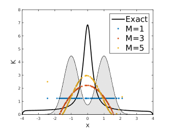
(a) Galerkin gain approxmiation for $N=100$

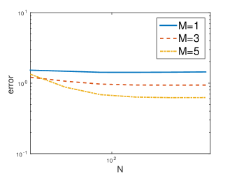
(b) Galerkin gain approx. error as a function of $N$

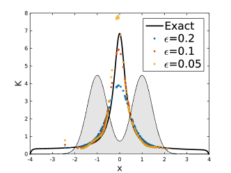
(c) Kernel-based gain approximation for $N=100$

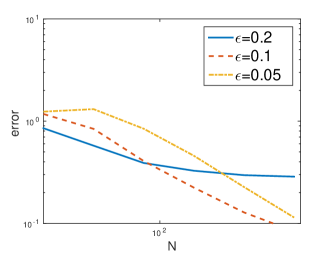
(d) Kernel-based gain approx. error as a function of $N$

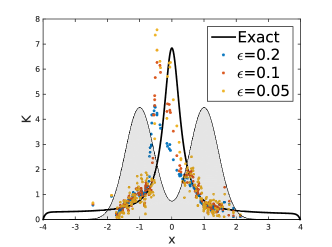
(e) Optimal Coupling gain approximation for $N=100$

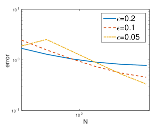
(f) Optimal Coupling gain approx. error as a function of $N$

Figure 4: Comparison of the gain function approximations obtained using Galerkin (part (a)), kernel (part (c)), and the optimal coupling (part (e)) algorithms. The exact gain function is depicted as a solid line and the density $\rho$ is depicted as a shaded region in the background. The parts (b)-(d)-(e) depict the Monte-Carlo estimate of the empirical error (26) as a function of the number of particles $N$. The Monte-Carlo estimate is obtained by averaging the empirical error over 100 simulations.

The following observations are made based on the results of these numerical experiments:

1. (Figure 4 (a)-(b)) The accuracy of the Galerkin algorithm improves as the number of basis function increases. For a fixed number of particles, the matrix $A$ becomes poorly conditioned as the number of basis functions becomes large. This can lead to numerical instabilities in solving the matrix equation (16).

2. (Figure 4 (a)-(c)-(d)) The kernel-based and optimal coupling algorithms, preserve the positivity property of the exact gain. The positivity property of the gain is not necesarily preserved in the Galerkin algorithm. The correct sign of the gain is important in filtering applications as the gain determines the direction of drift of the particles. A wrong sign can lead to divergence of the particle trajectories.

3. (Figure 5) For a fixed number of particles, there is an optimal value of $\epsilon$ that minimizes the error for the kernel-based and the optimal coupling algorithms. For the kernel-based algorithm, it is shown in [41] that, for small $\epsilon$ and large $N$, the error scales as $O(\epsilon)+O(\frac{1}{\epsilon^{d/2+1}\sqrt{N}})$. As $\epsilon\rightarrow\infty$, the approximate gain converges to the constant gain approximation. In particular, the error remains bounded even for large values of $\epsilon$.

4. The optimal coupling algorithm leads to spatially more irregular approximations which nevertheless converge as the number of particles increases. The optimal choice of the parameter $\epsilon$ depends on the particle size. Finally, a spatially more regular approximation could be obtained using kernel dressing, e.g., by convoluting the particle approximation with Gaussian kernels.

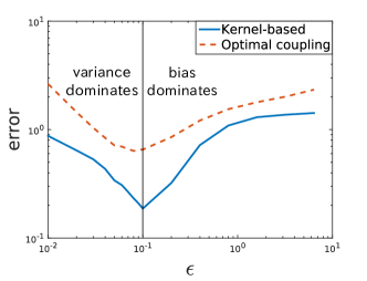
Figure 5: Comparison of the Monte-Carlo estimate of the empirical error (26) as a function of the parameter $\epsilon$. The number of particles $N=200$.

7 Conclusion

We have summarized an interacting particle representation of the classic Kalman-Bucy filter and its extension to nonlinear systems and non-Gaussian distributions under the general framework of FPFs. This framework is attractive since it maintains key structural elements of the classic Kalman-Bucy filter, namely, a gain factor and the innovation. In particular, the EnKF has become widely used in data assimilation for atmosphere-ocean dynamics and oil reservoir exploration. Robust extensions of the EnKF to non-Gaussian distributions are urgently needed and FPFs provide a systematic approach for such extensions in the spirit of Kalman’s original work. However, interacting particle representations come at a price; they require approximate solutions of an elliptic PDE or a coupling problem, when viewed from a probabilistic perspective. Hence, robust and efficient numerical techniques for FPF-based interacting particle systems and study of their long-time behavior will be a primary focus of future research.

8 Acknowledgement

The first author AT was supported in part by the Computational Science and Engineering (CSE) Fellowship at the University of Illinois at Urbana-Champaign (UIUC). The research of AT and PGM at UIUC was additionally supported by the National Science Foundation (NSF) grants 1334987 and 1462773. This support is gratefully acknowledged. The research of JdW and SR has been partially funded by Deutsche Forschungsgemeinschaft (DFG) through the grant CRC 1114 “Scaling Cascades in Complex Systems”, Project (A02) “Multiscale data and asymptotic model assimilation for atmospheric flows” and the grant CRC 1294 “Data Assimilation”, Project (A02) “Long-time stability and accuracy of ensemble transform filter algorithms”.

Appendix A Exactness of the Feedback Particle Filter

The objective of this section is to describe the consistency result for the feedback particle algorithm (9), in the sense that the posterior distribution of the particle exactly matches the posterior distribution in the mean-field limit as $N\to\infty$. To put this in a mathematical framework, let $\pi^{*}_{t}$ denote the conditional distribution of $X_{t}\in{\cal X}$ given history (filtration) of observations $\mathcal{Z}_{t}:=\sigma\{Z_{s},s\leq t\}$. For a real-valued function $f:{\cal X}\to\mathbb{R}$ define the action of $\pi^{*}_{t}$ on $f$ according to:

$$\pi^{*}_{t}(f):={\sf E}[f(X_{t})|{\cal Z}_{t}]$$

The time evolution of $\pi^{*}_{t}(f)$ is described by Kushner-Stratonovich pde (see Theorem 5.7 in [42]),

$$\pi^{*}_{t}(f)= \pi^{*}_{0}(f)+\int_{0}^{t}\pi^{*}_{s}(\mathcal{L}f)\,\mathrm{d}s$$ (27)

$$+\int_{0}^{t}\left(\pi^{*}_{s}(fh)-\pi^{*}_{s}(f)\pi^{*}_{s}(f)\right)\left(\,\mathrm{d}Z_{s}-\pi_{s}^{*}(h)\,\mathrm{d}s\right)$$

where $f\in C^{\infty}_{c}({\cal X})$ (smooth functions with compact support), and

$$\mathcal{L}f:=a(x)\cdot\nabla f(x)+\frac{1}{2}\sum_{k,l=1}^{d}\sigma_{k}(x)\sigma_{l}(x)\frac{\partial^{2}f}{\partial x_{k}\partial x_{l}}(x)$$

Next define $\pi_{t}$ to be the conditional distribution of $X^{i}_{t}\in{\cal X}$ given ${\cal Z}_{t}$. It’s action on real-valued function is defined according to:

$$\pi_{t}(f):={\sf E}[f(X^{i}_{t})|{\cal Z}_{t}]$$

The time evolution of $\pi_{t}(f)$ is described by the Fokker-Planck equation (see Proposition 1 in [31]):

$$\pi_{t}(f)= \pi_{0}(f)+\int_{0}^{t}\pi_{s}(\mathcal{L}f)\,\mathrm{d}s+\int_{0}^{t}\pi_{s}({\sf K}\cdot\nabla f)\,\mathrm{d}Z_{s}$$ (28)

$$+\int_{0}^{t}\pi_{s}(u\cdot\nabla f)\,\mathrm{d}s+\frac{1}{2}\int_{0}^{t}\pi_{s}({\sf K}\cdot\nabla({\sf K}\cdot\nabla f))\,\mathrm{d}s$$

where ${\sf K}$ is the gain function and $u$ is the control function as follows:

1) Gain function: Let $\phi\in H^{1}({\cal X};\pi_{t})$ be the solution of a (weak form of the) Poisson equation:

$$\pi_{t}\big{(}\nabla\phi\cdot\nabla\psi\big{)}=\pi_{t}\big{(}(h-\pi_{t}(h))\psi\big{)}$$ (29)

$$\pi_{t}(\phi)=0~{}~{}~{}~{}(\text{mean-zero})$$

for all $\psi\in H^{1}(\mathcal{X};\pi_{t})$. The gain function ${\sf K}(x,t)=\nabla\phi(x)$.

2) Control function: The function $u(x,t)=-\frac{1}{2}\,{\sf K}(x,t)\,\big{(}h(x)+\pi_{t}(h)\big{)}$.

The existence-uniqueness of the gain function ${\sf K}$ requires additional assumptions on the distribution $\pi_{t}$ and the function $h$.

• Assumption A1: The probability distribution $\pi_{t}$ admits a spectral gap. That is , $\exists\,\lambda>0$ such that for all functions $f\in H^{1}_{0}({\cal X},\pi_{t})$,

  $$\pi_{t}(|f|^{2})\leq\frac{1}{\lambda}\pi_{t}(|\nabla f|^{2})$$

  for $t\in[0,T]$.

• Assumption A2: The function $h\in L^{2}({\cal X};\pi_{t})$, the space of square-integrable functions with respect to $\pi_{t}$.

Under the Assumptions (A1) and (A2) the Poisson equation (29) has a unique solution $\phi\in H^{1}_{0}(\mathcal{X},\pi_{t})$ and the resulting control and gain function will be admissible [31]. The consistency of the feedback particle filter is stated in the following Theorem.

Theorem 1

Let $\pi^{*}_{t}$ and $\pi_{t}$ satisfy the forward equations (27) and (28), respectively. Then assuming $\pi^{*}_{0}=\pi_{0}$, we have:

$$\pi^{*}_{t}(f)=\pi_{t}(f)$$ (30)

for all $t\in[0,T]$ and all functions $f\in C^{\infty}_{c}(\mathbb{R}^{d})$.

Proof A.2.

Using (27) and (28) it is sufficient to show the following two identities:

$$\pi_{s}({\sf K}\cdot\nabla f) =\pi_{s}(fh)-\pi_{s}(f)\pi_{s}(h)$$

$$\pi_{s}(u\cdot\nabla f)+\frac{1}{2}\pi_{s}({\sf K}\cdot\nabla({\sf K}\cdot\nabla f)) =-\left(\pi_{s}(fh)-\pi_{s}(f)\pi_{s}(h)\right)\pi_{s}(h)$$

The first identity is obtained by using ${\sf K}=\nabla\phi$ and the weak form of the Poisson equation (29) with $\psi=f$. The second identity is obtained similarly. Use the expression for the control function $u$ to obtain,

$$\pi_{s}(u\cdot\nabla f) =-\pi_{s}(\frac{h+\pi_{s}(h)}{2}{\sf K}\cdot\nabla f)$$

$$=-\frac{1}{2}\pi_{s}((h-\pi_{s}(h)){\sf K}\cdot\nabla f)-\pi_{s}(h)\pi_{s}({\sf K}\cdot\nabla f)$$

$$=-\frac{1}{2}({\sf K}\cdot\nabla({\sf K}\cdot\nabla f))-\pi_{s}(h)\pi_{s}((h-\pi_{s}(h))f)$$

where in the last step the weak form of the Poisson equation (29) is used for the $\psi={\sf K}\cdot\nabla f$ and $\psi=f$. This concludes the second identity and hence the Theorem.

Appendix B Relationship of gain function to the optimal transport map

Let $S_{\epsilon}$ be the optimal transport map, solution of the problem (23). It is known that this map is of a gradient form [32]. In the following we furthermore assume that the map $S_{\epsilon}=:\nabla\Phi_{\epsilon}$ is $C^{1}$ in the parameter $\epsilon$. For any test function $\psi$

$$C_{\epsilon}=\int\psi(\nabla\Phi_{\epsilon}(x))\rho(x)\,\mathrm{d}x-\int\psi(x)\rho_{\epsilon}(x)\,\mathrm{d}x\equiv 0$$

Therefore,

$$\left.\frac{\,\mathrm{d}C_{\epsilon}}{\,\mathrm{d}\epsilon}\right|_{\epsilon=0}=\int\nabla\phi(x)\cdot\nabla\psi(x)\rho(x)\,\mathrm{d}x-\int(h(x)-\hat{h})\psi(x)\rho(x)\,\mathrm{d}x=0$$

where $\phi:=\frac{\,\mathrm{d}\Phi_{\epsilon}}{\,\mathrm{d}\epsilon}\big{|}_{\epsilon=0}$. This is the weak form of the Poisson equation (10). Therefore,

$${\sf K}=\nabla\phi=\frac{\,\mathrm{d}S_{\epsilon}}{\,\mathrm{d}\epsilon}\bigg{|}_{\epsilon=0}$$

References

- [1] Kalnay, E., 2002. Atmospheric Modeling, Data Assimilation and Predictability. Cambridge University Press.
- [2] Oliver, D., Reynolds, A., and Liu, N., 2008. Inverse theory for petroleum reservoir characterization and history matching. Cambridge University Press, Cambridge.
- [3] Kitanidis, P., 1995. “Quasi-linear geostatistical theory for inversion”. Water Resources Research, 31, pp. 2411–2419.
- [4] Burgers, G., van Leeuwen, P., and Evensen, G., 1998. “On the analysis scheme in the ensemble Kalman filter”. Mon. Wea. Rev., 126, pp. 1719–1724.
- [5] Houtekamer, P., and Mitchell, H., 2001. “A sequential ensemble Kalman filter for atmospheric data assimilation”. Mon. Wea. Rev., 129, pp. 123–136.
- [6] Julier, S. J., and Uhlmann, J. K., 1997. “A new extension of the Kalman filter to nonlinear systems”. In Signal processing, sensor fusion, and target recognition. Conference No. 6, Vol. 3068, pp. 182–193.
- [7] Reich, S., and Cotter, C., 2015. Probabilistic Forecasting and Bayesian Data Assimilation. Cambridge University Press, Cambridge, UK.
- [8] Daum, F., Huang, J., and Noushin, A., 2010. “Exact particle flow for nonlinear filters”. In SPIE Defense, Security, and Sensing, pp. 769704–769704.
- [9] Daum, F., Huang, J., and Noushin, A., 2017. “Generalized gromov method for stochastic particle flow filters”. In SPIE Defense+ Security, International Society for Optics and Photonics, pp. 102000I–102000I.
- [10] Ma, R., and Coleman, T. P., 2011. “Generalizing the posterior matching scheme to higher dimensions via optimal transportation”. In Communication, Control, and Computing (Allerton), 2011 49th Annual Allerton Conference on, pp. 96–102.
- [11] El Moselhy, T. A., and Marzouk, Y. M., 2012. “Bayesian inference with optimal maps”. Journal of Computational Physics, 231(23), pp. 7815–7850.
- [12] Heng, J., Doucet, A., and Pokern, Y., 2015. “Gibbs Flow for Approximate Transport with Applications to Bayesian Computation”. ArXiv e-prints, Sept.
- [13] Yang, T., Blom, H., and Mehta, P. G., 2014. “The continuous-discrete time feedback particle filter”. In American Control Conference (ACC), 2014, IEEE, pp. 648–653.
- [14] Crisan, D., and Xiong, J., 2007. “Numerical solutions for a class of SPDEs over bounded domains”. ESAIM: Proc., 19, pp. 121–125.
- [15] Crisan, D., and Xiong, J., 2010. “Approximate McKean-Vlasov representations for a class of SPDEs”. Stochastics, 82(1), pp. 53–68.
- [16] Yang, T., Mehta, P. G., and Meyn, S. P., 2011. “Feedback particle filter with mean-field coupling”. In Decision and Control and European Control Conference (CDC-ECC), 50th IEEE Conference on, pp. 7909–7916.
- [17] Yang, T., Mehta, P. G., and Meyn, S. P., 2013. “Feedback particle filter”. IEEE Trans. Automatic Control, 58(10), October, pp. 2465–2480.
- [18] Blom, H. A. P., 2012. “The continuous time roots of the interacting multiple model filter”. In Proc. 51st IEEE Conf. on Decision and Control, pp. 6015–6021.
- [19] Bar-Shalom, Y., Daum, F., and Huang, J., 2009. “The probabilistic data association filter”. IEEE Control Syst. Mag., 29(6), Dec, pp. 82–100.
- [20] Kalman, R. E., 1960. “A new approach to linear filtering and prediction problems”. Journal of basic Engineering, 82(1), pp. 35–45.
- [21] Law, K., Stuart, A., and Zygalakis, K., 2015. Data Assimilation: A Mathematical Introduction. Springer-Verlag, New York.
- [22] Reich, S., 2011. “A dynamical systems framework for intermittent data assimilation”. BIT Numerical Analysis, 51, pp. 235–249.
- [23] Bergemann, K., and Reich, S., 2012. “An ensemble Kalman-Bucy filter for continuous data assimilation”. Meteorolog. Zeitschrift, 21, pp. 213–219.
- [24] de Wiljes, J., Reich, S., and Stannat, W., 2016. Long-time stability and accuracy of the ensemble Kalman-Bucy filter for fully observed processes and small measurement noise. Tech. Rep. https://arxiv.org/abs/1612.06065, University Potsdam.
- [25] Del Moral, P., Kurtzmann, A., and Tugaut, J., 2016. On the stability and the uniform propagation of chaos of extended ensemble Kalman-Bucy filters. Tech. Rep. arXiv:1606.08256v1, INRIA Bordeaux Research Center.
- [26] Kelly, D., Law, K., and Stuart, A., 2014. “Well-posedness and accuracy of the ensemble Kalman filter in discrete and continuous time”. Nonlinearity, 27(10), p. 2579.
- [27] Kelly, D., and Stuart, A. M., 2016. Ergodicity and accuracy of optimal particle filters for Bayesian data assimilation. Tech. Rep. https://arxiv.org/abs/1611.08761, Courant Institute of Mathematical Sciences.
- [28] Kelly, D., Majda, A. J., and Tong, X. T., 2015. “Concrete ensemble Kalman filters with rigorous catastrophic filter divergence”. PNAS.
- [29] Oksendal, B., 2013. Stochastic differential equations: an introduction with applications. Springer Science & Business Media.
- [30] Zhang, C., Taghvaei, A., and Mehta, P. G., 2016. “Feedback particle filter on matrix Lie groups”. In American Control Conference (ACC), 2016, IEEE, pp. 2723–2728.
- [31] Yang, T., Laugesen, R. S., Mehta, P. G., and Meyn, S. P., 2016. “Multivariable feedback particle filter”. Automatica, 71, pp. 10–23.
- [32] Villani, C., 2003. Topics in Optimal Transportation. No. 58. American Mathematical Soc.
- [33] Evans, L. C., 1997. “Partial differential equations and Monge-Kantorovich mass transfer”. Current developments in mathematics, pp. 65–126.
- [34] Laugesen, R. S., Mehta, P. G., Meyn, S. P., and Raginsky, M., 2015. “Poisson’s equation in nonlinear filtering”. SIAM J. Control Optim., 53(1), pp. 501–525.
- [35] Stano, P. M., Tilton, A. K., and Babuška, R., 2014. “Estimation of the soil-dependent time-varying parameters of the hopper sedimentation model: The FPF versus the BPF”. Control Engineering Practice, 24, pp. 67–78.
- [36] Tilton, A. K., Ghiotto, S., and Mehta, P. G., 2013. “A comparative study of nonlinear filtering techniques”. In Information Fusion (FUSION), 2013 16th International Conference on, pp. 1827–1834.
- [37] Berntorp, K., 2015. “Feedback particle filter: Application and evaluation”. In 18th Int. Conf. Information Fusion, Washington, DC.
- [38] Berntorp, K., and Grover, P., 2016. “Data-driven gain computation in the feedback particle filter”. In 2016 American Control Conference (ACC), IEEE, pp. 2711–2716.
- [39] Coifman, R. R., and Lafon, S., 2006. “Diffusion maps”. Appl. Comput. Harmon. A., 21(1), pp. 5–30.
- [40] Hein, M., Audibert, J., and Luxburg, U., 2007. “Graph Laplacians and their convergence on random neighborhood graphs”. J. Mach. Learn. Res., 8(Jun), pp. 1325–1368.
- [41] Taghvaei, A., Mehta, P. G., and Meyn, S. P., 2017. “Error estimates for the kernel gain function approximation in the feedback particle filter”. In American Control Conference (ACC), 2017, IEEE, pp. 4576–4582.
- [42] Xiong, J., 2008. An introduction to stochastic filtering theory, Vol. 18 of Oxford Graduate Texts in Mathematics. Oxford University Press.