Semi-leptonic $B$-physics anomalies:
a general EFT analysis within $U(2)^{n}$ flavor symmetry

Abstract

We analyse the recent hints of Lepton Flavor Universality violations in semi-leptonic $B$ decays within a general EFT based on a $U(2)^{n}$ flavor symmetry acting on the light generations of SM fermions. We analyse in particular the consistency of these anomalies with the tight constraints on various low-energy observables in $B$ and $\tau$ physics. We show that, with a moderate fine-tuning, a consistent picture for all low-energy observables can be obtained under the additional dynamical assumption that the NP sector is coupled preferentially to third generation SM fermions. We discuss how this dynamical assumption can be implemented in general terms within the EFT, and we identify a series of observables in $\tau$ decays which could provide further evidences of this NP framework.

1 Introduction

The hints of Lepton Flavor Universality (LFU) violations in semi-leptonic $B$ decays are among the most interesting and persisting deviations from the Standard Model (SM) reported by experiments in the last few years. The statistically most significant results are encoded by the following three ratios:

$$R^{\tau/\ell}_{D^{*}} = \frac{\mathcal{B}(B\to D^{*}\tau\overline{\nu})_{\rm exp}/\mathcal{B}(B\to D^{*}\tau\overline{\nu})_{\rm SM}}{\mathcal{B}(B\to D^{*}\ell\overline{\nu})_{\rm exp}/\mathcal{B}(B\to D^{*}\ell\overline{\nu})_{\rm SM}}=1.23\pm 0.07~{},$$ (1)

$$R^{\tau/\ell}_{D} = \frac{\mathcal{B}(B\to D\tau\overline{\nu})_{\rm exp}/\mathcal{B}(B\to D\tau\overline{\nu})_{\rm SM}}{\mathcal{B}(B\to D\ell\overline{\nu})_{\rm exp}/\mathcal{B}(B\to D\ell\overline{\nu})_{\rm SM}}=1.34\pm 0.17~{},$$ (2)

$$R^{\mu/e}_{K} = \left.\frac{\mathcal{B}(B\to K\mu\overline{\mu})_{\rm exp}}{\mathcal{B}(B\to Ke\overline{e})_{\rm exp}}\right|_{q^{2}\in[1,6]{\rm GeV}}=0.745{}^{+0.090}_{-0.074}\pm 0.036~{},$$ (3)

where $\ell$ generically denotes a light lepton ($\ell=e,\mu$).

In addition to these LFU ratios, whose deviation from unity would clearly signal physics beyond the SM, semi-leptonic $B$ decay data exhibit other tensions with the SM predictions. Most notably, a deviation of about $3\sigma$ has been reported by LHCb [9] on the so-called $P_{5}^{\prime}(B\to K^{*}\mu\overline{\mu})$ differential observable. This result is also compatible with recent Belle data [10], although the latter have a smaller statistical significance. The $P_{5}^{\prime}$ anomaly alone is not an unambiguous signal of new physics, given the non-negligible uncertainties affecting its SM prediction [11]. However, it is interesting to note that all available $b\to s\ell\overline{\ell}$ data (including the ratio $R^{\mu/e}_{K}$ reported above) turn out to be in better agreement with the corresponding theory predictions under the assumption of a single lepton-flavor non-universal short-distance amplitude affecting only the muonic modes (for an updated discussion see e.g. Ref. [12, 13, 14] and references therein).

These deviations from the SM have triggered a series of theoretical speculations about possible New Physics (NP) interpretations. In particular, attempts to provide a combined/coherent explanation for both charged- and neutral-current anomalies have been presented in Ref. [15, 16, 17, 18, 19, 20, 21, 22, 23, 24, 25, 26]. Among them, a particularly interesting class is that of models based on a $U(2)^{n}$ flavor symmetry, acting on the light generations of SM fermions [27, 28], and new massive vector mediators around the TeV scale (either colorless $SU(2)_{L}$ triplets [17], or $SU(2)_{L}$ doublet leptoquarks [21]). Beside providing a good description of low-energy data, these mediators could find a consistent UV completion in the context of strongly-interacting theories with new degrees of freedom at the TeV scale [29, 30].

While these NP interpretations are quite interesting, their compatibility with high-$p_{T}$ data from the LHC and other precision low-energy observables is not trivial. On the one hand, it has been pointed out that high-$p_{T}$ searches of resonances decaying into a $\tau\overline{\tau}$ pair ($pp\to\tau\overline{\tau}+X$) represent a very stringent constraint for virtually any model addressing the $R^{\tau/\ell}_{D^{(}*)}$ anomalies [31]. On the other hand, the consistency with LFU tests and the bounds on Lepton Flavor Violation (LFV) from $\tau$ decays, after taking into account quantum corrections, seems to be problematic [32]. Last but not least, in all the explicit models constructed so far, a non-negligible amount of fine-tuning seems to be unavoidable in order to satisfy the constraints from $B_{s}$ and $B_{d}$ meson-antimeson mixing (see, in particular, Ref. [21, 29]).

The compatibility with collider searches is certainly a serious issue; however, it should not be over-emphasized especially in the context of strongly interacting theories, where the extrapolation from low-energy data to the on-shell production of the new states is subject to sizable uncertainties. On the contrary, the compatibility of these anomalies with other low-energy data is a question that can be addressed in a model-independent way using an appropriate Effective Field Theory (EFT) approach. The purpose of this paper is to revisit the consistency and the compatibility of the anomalies reported in Eqs. (1)–(3) with other low-energy data, employing a general EFT approach based on the $U(2)^{n}$ flavor symmetry.

As it appeared clear from the first $U(2)^{n}$ based analyses [17, 21], the flavor symmetry alone is not enough to guarantee a natural explanation of $B$-physics anomalies in a general EFT approach. Additional dynamical assumptions are needed to explained the observed hierarchy among the various effective operators. Our goal is to discuss in general terms possible power-counting schemes to justify these hierarchies and, within such schemes, to quantify the amount of fine-tuning necessary to obtain a satisfactory description of all low-energy data.

The paper is organised as follows. In Section 2 we define the low-energy EFT and provide a complete list of the four-fermion operators with the inclusion of at most one lepton spurion and one (or two) quark spurion(s) contributing to $\Delta F=1$ (or $\Delta F=2$) processes. The bounds on these operators from the relevant low-energy observables are discussed in Section 3. In Section 4.1 we analyse these bounds and determine a consistent power-counting scheme that allow us justify the observed hierarchies. In Section 4.2 we discuss selected observables receiving leading contributions from operators with two lepton spurions (among which $R^{\mu/e}_{K}$), further testing the consistency of the proposed power-counting scheme. The final results, with a quantification of the fine-tuning needed to reconcile anomalies and bounds, are summarised in the Conclusions.

2 Setup

The EFT we are considering is characterised by the SM field content, the SM gauge symmetry ($SU(3)_{c}\times SU(2)_{L}\times U(1)_{Y}$), and a global flavor symmetry ${\mathcal{G}}_{\rm flavor}$, that we can decompose as follows

$${\mathcal{G}}_{\rm flavor}=U(2)_{q}\times U(2)_{\ell}\times{\mathcal{G}}_{R}~{}.$$ (4)

The left-handed SM fermions ($q^{i}_{L}$ and $\ell^{i}_{L}$) are singlets under ${\mathcal{G}}_{R}$ and have the following transformation properties under $U(2)_{q}\times U(2)_{\ell}$:

$$Q\equiv(q^{1}_{L},q^{2}_{L})\sim(2,1)~{},\qquad q_{3L}\equiv q^{3}_{L}\sim(1,1)~{},$$ (5)

$$L\equiv(\ell^{1}_{L},\ell^{2}_{L})\sim(1,2)~{},\qquad\ell_{3L}\equiv\ell^{3}_{L}\sim(1,1)~{}.$$ (6)

The third-generation right-handed fermions ($t_{R}$, $b_{R}$ and $\tau_{R}$) are all singlets of the complete group ${\mathcal{G}}_{\rm flavor}$. Various options are possible as far as the action of ${\mathcal{G}}_{\rm flavor}$ on the right-handed light-generation fermions is concerned. The simplest choice is the MFV-like [33] setting ${\mathcal{G}}_{R}=U(2)_{u_{R}}\times U(2)_{d_{R}}\times U(2)_{e_{R}}$, such that $E=(\mu_{R},e_{R})$ transforms as a doublet of $U(2)_{e_{R}}$, and similarly for right-handed light quarks. But other options, where $\mu_{R}$ and $e_{R}$ belong to the same non-trivial representation of a non-Abelian subgroup, leads to equivalent results.

We further consider two breaking spurions of the flavor symmetry, $V_{Q}$ and $V_{L}$, transforming, respectively, as (2,1) and (1,2) of $U(2)_{q}\times U(2)_{\ell}$. The structure of $V_{Q}$ can be connected to the CKM matrix ($V$) up to an overall normalization factor [27]:

$$V_{Q}\equiv(V_{Q_{1}},V_{Q_{2}})=|V_{Q}|\times\left(\frac{V^{*}_{td}}{V^{*}_{ts}},1\right),$$ (7)

with $|V_{Q}|$ expected to be of $O(|V_{ts}|)$. In the case of $V_{L}$, in the absence of a clear connection to the entries in the lepton Yukawa couplings, and given the strong universality bounds in processes involving electrons, we assume the following hierarchical structure:

$$V_{L}\equiv(V_{L_{1}},V_{L_{2}})=|V_{L}|\times\left(0,1\right)~{},$$ (8)

with $|V_{L}|\ll 1$ (an estimate of the maximal allowed value for $|V_{L_{1}}/V_{L_{2}}|$ is presented in Section 4.3).

So far we have not specified the flavor basis of the left-handed fermion doublets, or better how we define the $U(2)_{q}\times U(2)_{\ell}$ singlets. In the lepton case, the natural choice is provided by the charged-lepton mass-eigenstate basis (or by identifying $\tau_{L}$ as the $U(2)_{\ell}$ singlet). In the quark sector the situation is more ambiguous. In principle, any linear combination between down- and up-quark mass eigenstates is equally valid. For the sake of simplicity, we assume as reference basis the down-quark mass-eigenstate basis. This corresponds to identifying the $U(2)_{q}$ singlet and doublet as

$$q_{3L}=\left(\begin{array}[]{c}V^{*}_{kb}u^{k}_{L}\\ b_{L}\end{array}\right)\qquad{\rm and}\qquad Q^{i}=\left(\begin{array}[]{c}V^{*}_{ki}u^{k}_{L}\\ d^{i}_{L}\end{array}\right)~{},\quad i=\{1,2\}\equiv\{d,s\}~{}.$$ (9)

A “natural” change of basis is equivalent to the following shift in $q_{3L}$

$$q_{3L}\to q^{\prime}_{3L}=\cos(\theta)q_{3L}+\sin(\theta)V^{\dagger}_{Qi}Q^{i}~{},$$ (10)

where $\theta$ is an arbitrary angle. As a result, we can consider natural (non fine-tuned) the EFT constructions if operators without spurions and corresponding terms obtained with the replacement $q_{3L}\to V^{\dagger}_{Qi}Q^{i}$ have coefficients of similar size.

	Operator	Relevant low-energy observables
$\mathcal{O}^{qq}_{01}$	$\left[\overline{q}_{3L}\gamma^{\mu}Q^{i}V^{\dagger}_{Qi}\right]^{2}$	$\Delta M_{B_{d}}$, $\Delta M_{B_{s}}$
$\mathcal{O}^{qq}_{02}$	$\left[\overline{q}_{3L}\sigma^{a}\gamma^{\mu}Q^{i}V^{\dagger}_{Qi}\right]^{2}$	$\Delta M_{B_{d}}$, $\Delta M_{B_{s}}$

Table 1: Four-quark operators contributing to $\Delta F=2$ amplitudes with at most two quark spurions.

2.1 The basis of effective operators

In addition to the symmetries discussed above, we impose the conservation of baryon and lepton number, and we consider higher-dimensional operators up to dimension six. The EFT we are considering can thus be written as

$$\mathcal{L}_{\rm EFT}=\mathcal{L}_{\rm SM}+\frac{4G_{F}}{\sqrt{2}}\sum_{i}C_{i}\mathcal{O}_{i}~{},$$ (11)

using the Fermi scale, $v_{F}=(4G_{F}/\sqrt{2})^{-1/2}\approx 174$ GeV, as overall dimensional normalization factor. With such choice we reabsorb the value of the EFT effective scale ($\Lambda$) inside the Wilson coefficients, whose natural size in absence of specific suppression factors is $O(v_{F}^{2}/\Lambda^{2})$.

The effective operators $\mathcal{O}_{i}$ can be separated into three main categories: i) operators with no fermion fields; ii) operators with two fermion fields (plus Higgs or gauge fields); iii) four-fermion operators. The first two categories contain a small number of operators and are not particularly interesting to the processes we are considering. Within the class of four-fermion operators we can identify four interesting sub-categories, whose lists of operators, with the inclusion of at most one lepton spurion and one quark spurion (or two quark spurions in the case of $\Delta F=2$ operators), are reported in Table 1–4. For each operator we indicate the low-energy processes that can provide the most stringent constraint.

In the case of semi-leptonic operators we do not list explicitly those with a pair of right-handed light quarks since they do not give rise to signatures different from those of the operators already listed and, in addition, can be assumed to be suppressed under natural dynamical assumptions. For similar reasons, despite we have explicitly listed in Table 3– 4 tensor operators, we will ignore their effects in the phenomenological analysis of $b\to c\tau\overline{\nu}$ and $b\to s\tau\overline{\tau}$ transitions.

	Operator	Relevant low-energy processes
$\mathcal{O}^{q}_{01}$	$\left(\overline{q}_{3L}\gamma^{\mu}q_{3L}\right)\left(\overline{\ell}_{3L}\gamma_{\mu}\ell_{3L}\right)$	— ($\nu_{\tau}N\to\nu_{\tau}N$, $\Upsilon\to\tau\overline{\tau}$)
$\mathcal{O}^{q}_{02}$	$\left(\overline{q}_{3L}\sigma^{a}\gamma^{\mu}q_{3L}\right)\left(\overline{\ell}_{3L}\sigma_{a}\gamma_{\mu}\ell_{3L}\right)$	$b\to c\tau\overline{\nu}$
$\mathcal{O}^{q}_{03}$	$\left(\overline{q}_{3L}\gamma^{\mu}q_{3L}\right)\left(\overline{L}_{i}\gamma_{\mu}L^{i}\right)$	— ($\nu_{\ell}N\to\nu_{\ell}N$, $\Upsilon\to\ell\overline{\ell}$)
$\mathcal{O}^{q}_{04}$	$\left(\overline{q}_{3L}\sigma^{a}\gamma^{\mu}q_{3L}\right)\left(\overline{L}_{i}\sigma_{a}\gamma_{\mu}L^{i}\right)$	$b\to c\mu\overline{\nu}$
$\mathcal{O}^{q}_{05}$	$\left(\overline{Q}_{i}\gamma^{\mu}Q^{i}\right)\left(\overline{\ell}_{3L}\gamma_{\mu}\ell_{3L}\right)$	— ($\nu_{\tau}N\to\nu_{\tau}N$, $\phi\to\tau\overline{\tau}$)
$\mathcal{O}^{q}_{06}$	$\left(\overline{Q}_{i}\sigma^{a}\gamma^{\mu}Q^{i}\right)\left(\overline{\ell}_{3L}\sigma_{a}\gamma_{\mu}\ell_{3L}\right)$	$\tau\to K\nu$, $D\to\tau\nu$
$\mathcal{O}^{q}_{07}$	$\left(\overline{Q}_{i}\gamma^{\mu}Q^{i}\right)\left(\overline{L}_{i}\gamma_{\mu}L^{i}\right)$	— ($\nu_{\ell}N\to\nu_{\ell}N$, $\phi\to\ell\overline{\ell}$)
$\mathcal{O}^{q}_{08}$	$\left(\overline{Q}_{i}\sigma^{a}\gamma^{\mu}Q^{i}\right)\left(\overline{L}_{i}\sigma_{a}\gamma_{\mu}L^{i}\right)$	$K\to\ell\overline{\nu}$, $K\to\pi\ell\overline{\nu}$, $\pi\to\ell\overline{\nu}$
$\mathcal{O}^{q}_{11}$	$\left(\overline{q}_{3L}\gamma^{\mu}Q^{i}V^{\dagger}_{Qi}\right)\left(\overline{\ell}_{3L}\gamma_{\mu}\ell_{3L}\right)$	$b\to s\tau\overline{\tau}$, $b\to s\nu\overline{\nu}$
$\mathcal{O}^{q}_{12}$	$\left(\overline{q}_{3L}\sigma^{a}\gamma^{\mu}Q^{i}V^{\dagger}_{Qi}\right)\left(\overline{\ell}_{3L}\sigma_{a}\gamma_{\mu}\ell_{3L}\right)$	$b\to c\tau\overline{\nu}$, $b\to s\tau\overline{\tau}$, $b\to s\nu\overline{\nu}$, $\tau\to K\nu$
$\mathcal{O}^{q}_{13}$	$\left(\overline{q}_{3L}\gamma^{\mu}Q^{i}V^{\dagger}_{Qi}\right)\left(\overline{L}_{i}\gamma_{\mu}L^{i}\right)$	$b\to s\ell\overline{\ell}$, $b\to s\nu\overline{\nu}$
$\mathcal{O}^{q}_{14}$	$\left(\overline{q}_{3L}\sigma^{a}\gamma^{\mu}Q^{i}V^{\dagger}_{Qi}\right)\left(\overline{L}_{i}\sigma_{a}\gamma_{\mu}L^{i}\right)$	$b\to s\ell\overline{\ell}$, $b\to s\nu\overline{\nu}$
$\mathcal{O}^{q}_{21}$	$\left(\overline{q}_{3L}\gamma^{\mu}q_{3L}\right)\left(\overline{\ell}_{3L}\gamma_{\mu}L^{i}V^{\dagger}_{Li}\right)$	$\Upsilon\to\tau\overline{\mu}$, $\eta_{b}\to\tau\mu$
$\mathcal{O}^{q}_{22}$	$\left(\overline{q}_{3L}\sigma^{a}\gamma^{\mu}q_{3L}\right)\left(\overline{\ell}_{3L}\sigma_{a}\gamma_{\mu}L^{i}V^{\dagger}_{Li}\right)$	$\Upsilon\to\tau\overline{\mu}$, $\eta_{b}\to\tau\mu$
$\mathcal{O}^{q}_{23}$	$\left(\overline{Q}_{i}\gamma^{\mu}Q^{i}\right)\left(\overline{\ell}_{3L}\gamma_{\mu}L^{i}V^{\dagger}_{Li}\right)$	$\tau\to\mu\rho$, $\tau\to\mu\omega$
$\mathcal{O}^{q}_{24}$	$\left(\overline{Q}_{i}\sigma^{a}\gamma^{\mu}Q^{i}\right)\left(\overline{\ell}_{3L}\sigma_{a}\gamma_{\mu}L^{i}V^{\dagger}_{Li}\right)$	$\tau\to\mu\rho$, $\tau\to\mu\omega$
$\mathcal{O}^{q}_{31}$	$\left(\overline{q}_{3L}\gamma^{\mu}Q^{i}V^{\dagger}_{Qi}\right)\left(\overline{\ell}_{3L}\gamma_{\mu}L^{i}V^{\dagger}_{Li}\right)$	$B_{s}\to\tau\overline{\mu}$
$\mathcal{O}^{q}_{32}$	$\left(\overline{q}_{3L}\sigma^{a}\gamma^{\mu}Q^{i}V^{\dagger}_{Qi}\right)\left(\overline{\ell}_{3L}\sigma_{a}\gamma_{\mu}L^{i}V^{\dagger}_{Li}\right)$	$B_{s}\to\tau\overline{\mu}$

Table 2: Semi-leptonic four-fermion operators, with only left-handed currents and at most one lepton and/or one quark spurion. The processes listed between brackets do not give appreciable bounds and are reported only for completeness.

In principle, the various effective operators mix under quantum corrections. However, as indicated in Eq. (11), we assume a rather low effective scale such that no large logarithms are involved in the renormalization-group (RG) evolution. This implies that in most cases these mixing effects can be neglected. The only exception are cases where an operator with a large coefficient (in particular those contributing to $R_{D^{(*)}}$) mixes into a strongly constrained one (such as those contributing to leptonic $\tau$ decays), as pointed out first in Ref. [32]. Since no large logarithms are involved, we take into account this effects directly at the matrix-element level (i.e. taking into account also one-loop matrix elements, when necessary).

	Operator	Relevant low-energy processes
$\mathcal{O}^{q}_{R1}$	$\left(\overline{q}_{3L}\gamma^{\mu}q_{3L}\right)\left(\overline{\tau}_{R}\gamma_{\mu}\tau_{R}\right)$	— ($\Upsilon\to\tau\overline{\tau}$)
$\mathcal{O}^{q}_{R2}$	$\left(\overline{q}_{3L}\gamma^{\mu}Q^{i}V^{\dagger}_{Qi}\right)\left(\overline{\tau}_{R}\gamma_{\mu}\tau_{R}\right)$	$b\to s\tau\overline{\tau}$
$\mathcal{O}^{q}_{R3}$	$\left(\overline{Q}_{i}\gamma^{\mu}Q^{i}\right)\left(\overline{\tau}_{R}\gamma_{\mu}\tau_{R}\right)$	— ($\tau N\to\tau N$)
$\mathcal{O}^{q}_{R4}$	$\left(\overline{q}_{3L}\gamma^{\mu}q_{3L}\right)\left(\overline{E}_{j}\gamma_{\mu}{E^{j}}\right)$	— ($\Upsilon\to\ell\overline{\ell}$)
$\mathcal{O}^{q}_{R5}$	$\left(\overline{q}_{3L}\gamma^{\mu}Q^{i}V^{\dagger}_{Qi}\right)\left(\overline{E}_{j}\gamma_{\mu}{E^{j}}\right)$	$b\to s\ell\overline{\ell}$
$\mathcal{O}^{q}_{R6}$	$\left(\overline{Q}_{i}\gamma^{\mu}Q^{i}\right)\left(\overline{E}_{j}\gamma_{\mu}{E^{j}}\right)$	— ($\phi\to\ell\overline{\ell}$)
$\mathcal{O}^{q}_{S1}$	$\left(\overline{\ell}_{3L}\tau_{R}\right)\left(\overline{b}_{R}q_{3L}\right)$	$b\to c\tau\overline{\nu}$
$\mathcal{O}^{q}_{S2}$	$\left(\overline{\ell}_{3L}\tau_{R}\right)\left(\overline{b}_{R}Q^{i}V^{\dagger}_{Qi}\right)$	$b\to c\tau\overline{\nu}$, $b\to s\tau\overline{\tau}$
$\mathcal{O}^{q}_{S3}$	$\left(\overline{L}_{i}V_{L}^{i}\tau_{R}\right)\left(\overline{b}_{R}q_{3L}\right)$	$\eta_{b}\to\tau\overline{\mu}$
$\mathcal{O}^{q}_{T1}$	$\left(\overline{\ell}_{3L}\sigma_{\mu\nu}\tau_{R}\right)\left(\overline{b}_{R}\sigma^{\mu\nu}q_{3L}\right)$	$b\to c\tau\overline{\nu}$
$\mathcal{O}^{q}_{T2}$	$\left(\overline{\ell}_{3L}\sigma_{\mu\nu}\tau_{R}\right)\left(\overline{b}_{R}\sigma^{\mu\nu}Q^{i}V^{\dagger}_{Qi}\right)$	$b\to c\tau\overline{\nu}$, $b\to s\tau\overline{\tau}$
$\mathcal{O}^{q}_{T3}$	$\left(\overline{L}_{i}V_{L}^{i}\sigma_{\mu\nu}\tau_{R}\right)\left(\overline{b}_{R}\sigma^{\mu\nu}q_{3L}\right)$	$b\to c\tau\overline{\nu}$

Table 3: Semi-leptonic four-fermion operators, with leptonic right-handed and scalar currents, and at most one lepton and/or one quark spurion.

	Operator	Relevant low-energy processes
$\mathcal{O}^{\ell}_{01}$	$\left(\overline{\ell}_{3L}\gamma^{\mu}\ell_{3L}\right)\left(\overline{\ell}_{3L}\gamma_{\mu}\ell_{3L}\right)$	— (flav. cons. leptonic curr.)
$\mathcal{O}^{\ell}_{02}$	$\left(\overline{\ell}_{3L}\sigma^{a}\gamma^{\mu}\ell_{3L}\right)\left(\overline{\ell}_{3L}\sigma_{a}\gamma_{\mu}\ell_{3L}\right)$	— (flav. cons. leptonic curr.)
$\mathcal{O}^{\ell}_{03}$	$\left(\overline{\ell}_{3L}\gamma^{\mu}\ell_{3L}\right)\left(\overline{L}_{i}\gamma_{\mu}L^{i}\right)$	— (flav. cons. leptonic curr.)
$\mathcal{O}^{\ell}_{04}$	$\left(\overline{\ell}_{3L}\sigma^{a}\gamma^{\mu}\ell_{3L}\right)\left(\overline{L}_{i}\sigma_{a}\gamma_{\mu}L^{i}\right)$	$\tau\to\ell\nu\overline{\nu}$
$\mathcal{O}^{\ell}_{11}$	$\left(\overline{\ell}_{3L}\gamma^{\mu}\ell_{3L}\right)\left(\overline{\ell}_{3L}\gamma_{\mu}L^{i}V^{\dagger}_{Li}\right)$	$\tau\to\ell\nu\overline{\nu}$
$\mathcal{O}^{\ell}_{12}$	$\left(\overline{\ell}_{3L}\sigma^{a}\gamma^{\mu}\ell_{3L}\right)\left(\overline{\ell}_{3L}\sigma_{a}\gamma_{\mu}L^{i}V^{\dagger}_{Li}\right)$	$\tau\to\ell\nu\overline{\nu}$
$\mathcal{O}^{\ell}_{13}$	$\left(\overline{\ell}_{3L}\gamma^{\mu}L^{i}V^{\dagger}_{Li}\right)\left(\overline{L}_{j}\gamma_{\mu}L^{j}\right)$	$\tau\to\ell\nu\overline{\nu}$, $\tau\to\ell^{\prime}\ell\overline{\ell}$
$\mathcal{O}^{\ell}_{14}$	$\left(\overline{\ell}_{3L}\sigma^{a}\gamma^{\mu}L^{i}V^{\dagger}_{Li}\right)\left(\overline{L}_{j}\sigma_{a}\gamma_{\mu}L^{j}\right)$	$\tau\to\ell\nu\overline{\nu}$, $\tau\to\ell^{\prime}\ell\overline{\ell}$
$\mathcal{O}^{\ell}_{R1}$	$\left(\overline{\ell}_{3L}\gamma^{\mu}\ell_{3L}\right)\left(\overline{E}_{j}\gamma_{\mu}{E^{j}}\right)$	— (flav. cons. leptonic curr.)
$\mathcal{O}^{\ell}_{R2}$	$\left(\overline{\ell}_{3L}\gamma^{\mu}L^{i}V^{\dagger}_{Li}\right)\left(\overline{E}_{j}\gamma_{\mu}{E^{j}}\right)$	$\tau\to\ell^{\prime}\ell\overline{\ell}$
$\mathcal{O}^{\ell}_{S1}$	$\left(\overline{\ell}_{3L}{E^{j}}\right)\left(\overline{E}_{j}\ell_{3L}\right)$	— (flav. cons. leptonic curr.)
$\mathcal{O}^{\ell}_{S2}$	$\left(\overline{\ell}_{3L}{E^{j}}\right)\left(\overline{E}_{j}L^{i}V^{\dagger}_{Li}\right)$	$\tau\to\ell^{\prime}\ell\overline{\ell}$
$\mathcal{O}^{\ell}_{T1}$	$\left(\overline{\ell}_{3L}\sigma_{\mu\nu}{E^{j}}\right)\left(\overline{E}_{j}\sigma^{\mu\nu}\ell_{3L}\right)$	— (flav. cons. leptonic curr.)
$\mathcal{O}^{\ell}_{T2}$	$\left(\overline{\ell}_{3L}\sigma_{\mu\nu}{E^{j}}\right)\left(\overline{E}_{j}\sigma^{\mu\nu}L^{i}V^{\dagger}_{Li}\right)$	$\tau\to\ell^{\prime}\ell\overline{\ell}$

Table 4: Four-lepton operators

3 Observables

In this Section, we analyse the main experimental constraints on the operators with at most one lepton spurion listed in the previous Section. These includes the non-vanishing constraints from $R_{D}$ and $R_{D^{*}}$, and a long series of bounds from $\Delta F=1$ and $\Delta F=2$ processes, and $\tau$ decays. The discussion of selected observables receiving leading contributions from operators with two lepton spurions is postponed to Section 4.2. Unless otherwise specified, the bounds should be interpreted as bounds on the $C_{i}$ at the scale $\Lambda$ (i.e. neglecting RG corrections between $\Lambda$ and the electroweak scale).

3.1 Semi-leptonic $b\rightarrow c$ transitions

3.1.1 $B\rightarrow D\ell\overline{\nu}_{\ell}$

From the operators in Table 2, the effective charged-current Lagrangian describing $b\to c$ semi-leptonic decays with light leptons is:

$$\mathcal{L}(b\rightarrow c\ell\overline{\nu}_{\ell})=-\frac{4G_{F}}{\sqrt{2}}V_{cb}\left(1+2C^{q}_{04}+2V_{Q_{s}}C^{q}_{14}\frac{V_{cs}}{V_{cb}}\right)(\overline{c}_{L}\gamma^{\mu}b_{L})(\overline{\ell}_{L}\gamma_{\mu}\nu_{\ell L}).$$ (12)

Since the structure of the Lagrangian in Eq. (12) is SM-like, the decay width of the process $B\to D\ell\overline{\nu}_{\ell}$ can simply written as

$$\Gamma(B\rightarrow D\ell\nu_{\ell})=\Gamma^{\rm SM}(B\rightarrow D\ell\nu_{\ell})^{\rm SM}\left|1+\delta_{D}\right|^{2}~{},\qquad\delta_{D}=2C^{q}_{04}+2V_{Q_{s}}C^{q}_{14}\frac{V_{cs}}{V_{cb}}~{}.$$ (13)

Using the SM prediction $\mathcal{B}(B\to D\mu\overline{\nu}_{\mu})^{\mathrm{SM}}=(2.28\pm 0.19)\ 10^{-2}$ [34], and the experimental result in Ref. [35], we derive the bound

$$\mbox{Re}\left(C^{q}_{04}+V_{Q_{s}}C^{q}_{14}\frac{V_{cs}}{V_{cb}}\right)=-0.008\pm 0.025\,,$$ (14)

which is compatible with the hypothesis of negligible NP effects in the light lepton channels.

3.1.2 $B\rightarrow D^{(*)}\tau\overline{\nu}_{\tau}$

The effective Lagrangian relevant to semi-leptonic $b\to c$ decays with $\tau$ leptons in the final state is

$$\mathcal{L}(b\rightarrow c\tau\overline{\nu}_{\tau})=-\frac{4G_{F}}{\sqrt{2}}V_{cb}\bigg{[} \left(1+2C^{q}_{02}+2V_{Q_{s}}C^{q}_{12}\frac{V_{cs}}{V_{cb}}\right)(\overline{c}_{L}\gamma^{\mu}b_{L})(\overline{\tau}_{L}\gamma_{\mu}\nu_{\tau})$$ (15)

$$+\left(C^{q}_{S1}+V_{Q_{s}}C^{q}_{S2}\frac{V_{cs}}{V_{cb}}\right)(\overline{c}_{L}b_{R})(\overline{\tau}_{R}\nu_{\tau L})\bigg{]}~{}.$$

Contrary to the light lepton case, in the $\tau$ channel also the scalar operators $\mathcal{O}^{q}_{S1(2)}$ do appear and the decay amplitudes (and corresponding differential decay widths) cannot be expressed as a simple re-scaling of the SM ones.

Expanding to first order in the NP contributions, the $B\rightarrow D^{(*)}\tau\overline{\nu}_{\tau}$ differential decay widths can be decomposed as

$$\frac{\text{d}\Gamma}{\text{d}q^{2}}(B\rightarrow D^{(*)}\tau\overline{\nu}_{\tau})=(1+2\Delta)\frac{\text{d}\Gamma}{\text{d}q^{2}}(B\rightarrow D^{(*)}\tau\overline{\nu}_{\tau})_{\rm SM}+\Delta_{\rm S}\frac{\text{d}\Gamma}{\text{d}q^{2}}(B\rightarrow D^{(*)}\tau\overline{\nu}_{\tau})_{\rm VS}+O(C_{i}^{2})~{},$$ (16)

with

$$\Delta=2~{}\mbox{Re}\left(C^{q}_{02}+2V_{Q_{s}}C^{q}_{12}\frac{V_{cs}}{V_{cb}}\right)~{},\qquad\Delta_{\rm S}=\mbox{Re}\left(C^{q}_{S1}+V_{Q_{s}}C^{q}_{S2}\frac{V_{cs}}{V_{cb}}\right)~{}.$$ (17)

Following Ref. [36], the two SM differential decay distribution can be written as

$$\frac{\text{d}\Gamma}{\text{d}q^{2}}(B\rightarrow D\tau\overline{\nu}_{\tau})_{\rm SM}= \frac{G_{F}^{2}\sqrt{\lambda}|V_{cb}|^{2}\left(m_{\tau}^{2}-q^{2}\right)^{2}}{384\pi^{3}m_{B}^{3}q^{6}}\left[3f_{0}^{2}(q^{2})m_{\tau}^{2}\left(m_{B}^{2}-m_{D}^{2}\right)^{2}+f_{+}^{2}\lambda\left(m_{\tau}^{2}+2q^{2}\right)\right]~{},$$ (18)

$$\frac{\text{d}\Gamma}{\text{d}q^{2}}(B\rightarrow D^{*}\tau\overline{\nu}_{\tau})_{\rm SM}= \frac{G_{F}^{2}\sqrt{\lambda}|V_{cb}|^{2}\left(m_{\tau}^{2}-q^{2}\right)^{2}}{384\pi^{3}m_{B}q^{6}}\bigg{[}F_{0}^{2}\ m_{B}^{2}\left(m_{\tau}^{2}+2q^{2}\right)$$

$$+ q^{2}\left(F_{\perp}^{2}+F_{\parallel}^{2}\right)\left(m_{\tau}^{2}+2q^{2}\right)+3F_{t}^{2}\ m_{B}^{2}\ m_{\tau}^{2}\bigg{]}~{}.$$ (19)

The non-standard term $\frac{\text{d}\Gamma}{\text{d}q^{2}}(B\rightarrow D^{(*)}\tau\overline{\nu}_{\tau})_{\rm VS}$ arise from the interference between the left-handed and the scalar operators. Its explicit expression in the $D$ and $D^{*}$ case is

$$\frac{\text{d}\Gamma}{\text{d}q^{2}}(B\rightarrow D\tau\overline{\nu}_{\tau})_{\rm VS}= \ \frac{f_{0}^{2}G_{F}^{2}\sqrt{\lambda}\ m_{\tau}|V_{cb}|^{2}\left(m_{B}^{2}-m_{D}^{2}\right)^{2}\left(m_{\tau}^{2}-q^{2}\right)^{2}}{64\pi^{3}m_{B}^{3}q^{4}(m_{b}-m_{c})}~{},$$ (20)

$$\frac{\text{d}\Gamma}{\text{d}q^{2}}(B\rightarrow D^{*}\tau\overline{\nu}_{\tau})_{\rm VS}= \ \frac{F_{t}^{2}G_{F}^{2}\sqrt{\lambda}\ m_{B}\ m_{\tau}|V_{cb}|^{2}\left(m_{\tau}^{2}-q^{2}\right)^{2}}{64\pi^{3}q^{4}(m_{b}+m_{c})}~{}.$$ (21)

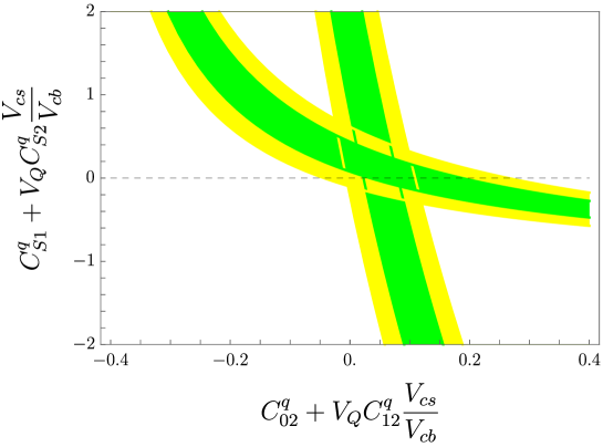
Figure 1: Parameter space allowed by the constraint on $\mathcal{B}(B\to D\tau\overline{\nu}_{\tau})$ and $\mathcal{B}(B\to D^{*}\tau\overline{\nu}_{\tau})$. The bands denotes 1 and $2\sigma$ limits (the $C_{i}$ are assumed to be real).

In principle, the best discrimination between scalar and left-handed contributions could be obtained by differential measurements of the two spectra, using the above formulae. So far these measurements are not available; however, a useful information can be derived also comparing the partial widths of two modes. The parameter space allowed by the experimental constraints [1] on $\mathcal{B}(B\to D\tau\nu_{\tau})$ and $\mathcal{B}(B\to D^{*}\tau\nu_{\tau})$ is shown in Fig. 1. As can be seen, the constraint on the scalar terms is quite weak. Still, it is interesting to note that present data are perfectly compatible with the absence of scalar terms, while pointing toward a non-negligible modification of the coefficient of the left-handed operator.

As anticipated in the Introduction, the ratios $R_{D^{(*)}}^{\tau/\mu}$, defined in Eqs. (1)–(2), play a crucial role in our analysis. Neglecting scalar terms, as suggested by Fig. 1, the parameter space allowed by these two ratios can easily be derived from Eqs. (13)–(16) and is shown in Fig. 2. If we further take in account the bound in Eq. (14), we deduce the following simple relation

$$\mbox{Re}\left(C^{q}_{02}+V_{Q_{2}}C^{q}_{12}\frac{V_{cs}}{V_{cb}}\right)=\frac{1}{4}\left[R_{D^{(*)}}^{\tau/\mu}-1\right],$$ (22)

which leads us to the following limits

$$\mbox{Re}\left(C^{q}_{02}+V_{Q_{2}}C^{q}_{12}\frac{V_{cs}}{V_{cb}}\right)~{}=~{}\left\{\begin{array}[]{l}0.06\pm 0.02\left[R_{D^{*}}\right]~{},\\ 0.09\pm 0.04\left[R_{D}\right]~{}.\end{array}\right.$$ (23)

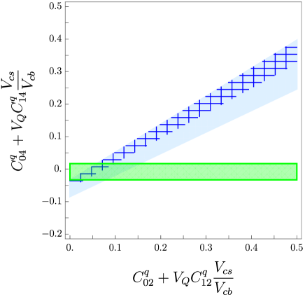
Figure 2: Parameter space allowed by the combination of the constraints given by the ratios $R_{D}$ (blue region) and $R_{D^{*}}$ (dashed region) in the hypothesis of negligible scalar current contributions. The horizontal band denotes the constraint from $\mathcal{B}(B\rightarrow D\mu\overline{\nu}_{\ell})$.

3.2 Semi-leptonic $s\rightarrow u$ transitions

The semi-leptonic operators listed in Table 2 generate also contributions to $s\to u$ transitions with $\tau$ and light leptons. The relevant effective Lagrangians, taking into account also the SM contributions, are

$$\mathcal{L}(s\to u\tau\nu) =-4\frac{G_{F}}{\sqrt{2}}V_{us}\left(1+2C^{q}_{06}+2C^{q}_{12}V_{Q_{s}}\frac{V_{ub}}{V_{us}}\right)(\overline{u}_{L}\gamma_{\mu}s_{L})(\overline{\tau}_{L}\gamma^{\mu}\nu_{\tau L})\,,$$ (24)

$$\mathcal{L}(s\to u\mu\nu) =-4\frac{G_{F}}{\sqrt{2}}V_{us}\left(1+2C^{q}_{08}+2C^{q}_{14}V_{Q_{s}}\frac{V_{ub}}{V_{us}}\right)(\overline{u}_{L}\gamma_{\mu}s_{L})(\overline{\mu}_{L}\gamma^{\mu}\nu_{\mu L})\,.$$ (25)

A particularly interesting observable to constrain the NP terms in these Lagrangians is the ratio $\mathcal{B}(\tau\to K\nu_{\tau})/\mathcal{B}(K\to\mu\overline{\nu}_{\mu})$, where the theoretical uncertainties on CKM elements and Kaon decay constant cancel out. Using the experimental results in [35] and the SM input in [37] we find

$$R_{sd}^{\tau/\mu}=\frac{\mathcal{B}(K\to\mu\overline{\nu}_{\mu})^{\rm exp}/\mathcal{B}(K\to\mu\overline{\nu}_{\mu})^{\rm SM}}{\mathcal{B}(\tau\to K\nu_{\tau})^{\rm exp}/\mathcal{B}(\tau\to K\nu_{\tau})^{\rm SM}}=1.029\pm 0.015~{},$$ (26)

which allows us to obtain the following bound

$$\mbox{Re}\left[C^{q}_{08}-C^{q}_{06}+\left(C^{q}_{14}-C^{q}_{12}\right)V_{Q_{s}}\frac{V_{ub}}{V_{us}}\right]=0.007\pm 0.004~{}.$$ (27)

It is worth to stress that $R_{sd}^{\tau/\mu}$ or, equivalently, the comparison of the $|V_{us}|$ determination from $\tau$ vs. $K$ decays is nothing but a test of LFU. Interestingly enough, present data exhibits a small tension with the SM prediction also in this case.

3.3 $\Delta F=2$ processes

According to the operators in Table 1, the effective Lagrangian relevant to $\Delta F=2$ processes is

$$\mathcal{L}^{\mathrm{NP}}_{\Delta F=2}=-\frac{4G_{F}}{\sqrt{2}}\left(C^{qq}_{01}+C^{qq}_{02}\right)(V^{*}_{Q_{i}})^{2}\left[\left(\overline{b}_{L}\gamma^{\mu}d^{i}_{L}\right)^{2}+\left(V^{*}_{ki}V_{j3}\right)^{2}\left(\overline{u}_{L}^{j}\gamma^{\mu}u_{L}^{k}\right)^{2}\right].$$ (28)

Since the structure of the effective operators is the same as in the SM, we can conveniently encode all the NP effects via the ratios

$$R_{B_{q}}^{\Delta F=2}=\frac{\mathcal{A}\left(B_{q}\to\overline{B}_{q}\right)_{\mathrm{SM+NP}}}{\mathcal{A}\left(B_{q}\to\overline{B}_{q}\right)_{\mathrm{SM}}}\qquad{\rm and}\qquad R_{D}^{\Delta F=2}=\frac{\mathcal{A}(D^{0}\to\overline{D}^{0})_{\mathrm{SM+NP}}}{\mathcal{A}(D^{0}\to\overline{D}^{0})_{\mathrm{SM}}}~{}.$$ (29)

In the $B$-physics case we find

$$R_{B_{q}}^{\Delta F=2}=1+\frac{\left(C^{qq}_{01}+C^{qq}_{02}\right)}{R_{\mathrm{SM}}^{\mathrm{loop}}}\left(\frac{V^{*}_{Q_{q}}}{V^{*}_{tb}V_{tq}}\right)^{2}~{},$$ (30)

where

$$R_{\mathrm{SM}}^{\mathrm{loop}}=\frac{\alpha_{em}}{16\pi s_{w}^{2}}S_{0}(x_{t})\eta_{B}\approx 1.6\times 10^{-3}~{}.$$ (31)

Given the flavor structure of $V_{Q_{i}}$, we get very similar bounds from $B_{d}$ and $B_{s}$ mixing, while the bound from $D^{0}$ is weaker. In particular, from the constraint $R_{B_{s}}\in\left(0.86,1.26\right)$ [39] we derive the bound

$$|V_{Q_{1}}|^{2}|C^{qq}_{01}+C^{qq}_{02}|<6.7\times 10^{-7}~{}.$$ (32)

3.4 FCNC $b\to s$ transitions

3.4.1 $B\to K^{(*)}\mu\overline{\mu}$

The Lagrangian that encodes FCNC $b\to s$ transition for the light lepton channels is

$$\mathcal{L}(b\rightarrow s\ell\overline{\ell})=-\frac{2G_{F}}{\sqrt{2}}\frac{\alpha_{e}}{2\pi}V_{ts}^{*}V_{tb}\left[\left(C_{9}+\Delta C_{9}\right)\mathcal{O}_{9}+\left(C_{10}+\Delta C_{10}\right)\mathcal{O}_{10}\right]~{},$$ (33)

where $\mathcal{O}_{9}$ and $\mathcal{O}_{10}$ are defined in Eq. (90) of Appendix B, and the shifts of $C_{9}$ and $C_{10}$ in term of the NP Wilson coefficients have the following form:

$$\Delta C_{9}= \frac{2\pi(C^{q}_{13}+C^{q}_{14}+C^{q}_{R5})V_{Q_{s}}}{\alpha_{e}V_{ts}^{*}V_{tb}}~{}, \Delta C_{10}= -\frac{2\pi(C^{q}_{13}+C^{q}_{14}-C^{q}_{R5})V_{Q_{s}}}{\alpha_{e}V_{ts}^{*}V_{tb}}~{}.$$ (34)

Inverting the relations above, we obtain an expression for the two combination of Wilson coefficients that appear in these channels as a function of the shifts $\Delta C_{9}$ and $\Delta C_{10}$. These shifts have been constrained in Ref. [12, 13, 14] from global fits of various $b\to s\mu\overline{\mu}$ observables (dominated by $B\to K^{*}\mu\overline{\mu}$ and $B\to K\mu\overline{\mu}$ data). Considering in particular the results in [12], namely $\Delta C_{9}=-1.05\pm 0.35$ and $\Delta C_{10}=0.3\pm 0.4$, we find

$$\mbox{Re}\left[(C^{q}_{13}+C^{q}_{14}+C^{q}_{R5})V_{Q_{s}}\right] =(-4.9\pm 1.7)\times 10^{-5}~{},$$ (35)

$$\mbox{Re}\left[(C^{q}_{13}+C^{q}_{14}-C^{q}_{R5})V_{Q_{s}}\right] =(1.4\pm 1.9)\times 10^{-5}~{}.$$ (36)

3.4.2 $B\rightarrow K^{(*)}\tau\overline{\tau}$

In principle, $b\to s\tau\overline{\tau}$ transitions would be excellent probes of our EFT construction. However, the current experimental bounds [40] are too weak to draw significant constraints. For completeness, and in view of future data, we report here the relevant formulae.

The relevant effective Lagrangian can be expressed as

$$\mathcal{L}(b\rightarrow s\tau\overline{\tau})=-\frac{2G_{F}}{\sqrt{2}}\frac{\alpha_{e}}{2\pi}V_{ts}^{*}V_{tb}\bigg{[}\left(C_{9}+\Delta C_{9}^{\tau}\right)\mathcal{O}_{9}+\left(C_{10}+\Delta C_{10}^{\tau}\right)\mathcal{O}_{10}+C_{S}^{\tau}(\mathcal{O}_{S}-\mathcal{O}_{P})\bigg{]},$$ (37)

where the operators $\mathcal{O}_{9}$, $\mathcal{O}_{10}$, $\mathcal{O}_{S}$ and $\mathcal{O}_{P}$ are defined in Eq. (90) with the identification $\ell=\tau$. In terms of the Wilson coefficients of the operators in Tables 2–3, the NP contributions are given by

$$\Delta C_{9(10)}^{\tau}= \pm\frac{2\pi(C^{q}_{11}+C^{q}_{12}\pm C^{q}_{R2})V_{Q_{s}}}{\alpha_{e}V_{ts}^{*}V_{tb}}~{}, C_{S}^{\tau}= \frac{2\pi C^{q}_{S2}V_{Q_{s}}}{\alpha_{e}V_{ts}^{*}V_{tb}}~{}.$$ (38)

3.4.3 $B\to K^{(*)}\nu\overline{\nu}$

From the operators in Table 2 we get the following Lagrangian for $b\to s\nu\overline{\nu}$ transitions

$$\mathcal{L}(b\to s\nu\overline{\nu})=-\frac{2G_{F}}{\sqrt{2}}\frac{\alpha_{e}}{2\pi}\left[\sum_{\ell=e,\mu}(C_{\nu}+\Delta C_{\nu_{\ell}})\mathcal{O}_{\nu_{\ell}}+(C_{\nu}+\Delta C_{\nu_{\tau}})\mathcal{O}_{\nu_{\tau}}\right]$$ (39)

where the operators $\mathcal{O}_{\nu_{\ell}}$ and $\mathcal{O}_{\nu_{\tau}}$ are defined starting from those in Eq. (90) as

$$\mathcal{O}_{\nu_{\ell}(\nu_{\tau})}=\left.\mathcal{O}_{9}-\mathcal{O}_{10}\right|_{\ell=\nu_{\ell}(\nu_{\tau})}~{}.$$ (40)

The shifts of the Wilson coefficients due to NP effects are

$$\Delta C_{\nu_{\ell}} =\frac{2\pi V_{Q_{2}}(C^{q}_{13}-C^{q}_{14})}{\alpha_{e}V_{ts}^{*}V_{tb}}~{}, \Delta C_{\nu_{\tau}} =\frac{2\pi V_{Q_{2}}(C^{q}_{11}-C^{q}_{12})}{\alpha_{e}V_{ts}^{*}V_{tb}}~{}.$$ (41)

Since the Lagrangian in Eq. (39) has a SM-like structure, the differential decay widths for $B\to K^{(*)}\nu\overline{\nu}$ decays can be expressed as

$$\frac{\mathrm{d}\Gamma}{\mathrm{d}q^{2}}(B\to K^{(*)}\nu\overline{\nu})=\frac{\mathrm{d}\Gamma}{\mathrm{d}q^{2}}(B\to K^{(*)}\nu\overline{\nu})^{\rm SM}\left|1+\frac{2}{3}\frac{\Delta C_{\nu_{\ell}}}{C_{\nu}}+\frac{1}{3}\frac{\Delta C_{\nu_{\tau}}}{C_{\nu}}\right|^{2}~{}.$$ (42)

In the case case, the SM spectrum can be be read from Eq. (B) setting $C_{9}=-C_{10}=C_{\nu}$, $C_{S}=$0 and $m_{\ell}=0$. Using the SM $C_{\nu}=-6.35$ [41] and the hadronic form factors in [42], from the experimental bound in [35] we obtain

$$-9.3<\mbox{Re}\left(\frac{\Delta C_{\nu_{\tau}}}{C_{\nu}}\right)<3.3\,,$$ (43)

in the limit $|\Delta C_{\nu_{\tau}}|\ll|\Delta C_{\nu}|$. This implies in turn

$$\mbox{Re}\left[V_{Q_{s}}(C^{q}_{11}-C^{q}_{12})\right]=(0.9\pm 1.8)\times 10^{-3}~{}.$$ (44)

3.5 Leptonic $\tau$ decays

3.5.1 $\tau\to\ell\nu\overline{\nu}$

The effective Lagrangian generating $\tau\to\mu\nu\overline{\nu}$ decay amplitudes at the tree level is

$$\mathcal{L}(\tau\to\mu\nu\overline{\nu})=-\frac{4G_{F}}{\sqrt{2}}\{ (1+2C^{\ell}_{04})(\overline{\nu}_{\tau_{L}}\gamma^{\lambda}\tau_{L})(\overline{\mu}_{L}\gamma_{\lambda}\nu_{\mu_{L}})+V_{L_{\mu}}[(3C^{\ell}_{12}-C^{\ell}_{11})(\overline{\nu}_{\tau_{L}}\gamma^{\lambda}\tau_{L})(\overline{\mu}_{L}\gamma_{\lambda}\nu_{\tau_{L}})$$ (45)

$$+ (3C^{\ell}_{14}-C^{\ell}_{13})(\overline{\nu}_{\mu_{L}}\gamma^{\lambda}\tau_{L})(\overline{\mu}_{L}\gamma_{\lambda}\nu_{\mu_{L}})+(C^{\ell}_{14}-C^{\ell}_{13})(\overline{\nu}_{e_{L}}\gamma^{\lambda}\tau_{L})(\overline{\mu}_{L}\gamma_{\lambda}\nu_{e_{L}})]\}.$$

Since the interacting structure is the same occurring within the SM, the decay width can be simply written as

$$\Gamma(\tau\to\mu\nu\overline{\nu})=\Gamma^{\rm SM}(\tau\to\mu\nu_{\tau}\overline{\nu}_{\mu})\times\left|1+2C^{\ell}_{04}\right|^{2}~{},$$ (46)

where $\Gamma^{\rm SM}(\tau\to\mu\nu_{\tau}\overline{\nu}_{\mu})$ is given in [37]. We can now consider the observable $R_{\tau}^{\tau/\ell}$, defined as

$$R_{\tau}^{\tau/\ell_{1,2}}=\frac{\mathcal{B}(\tau\to\ell_{2,1}\nu\overline{\nu})_{\mathrm{exp}}/\mathcal{B}(\tau\to\ell_{2,1}\nu\overline{\nu})_{\mathrm{SM}}}{\mathcal{B}(\mu\to e\nu\overline{\nu})_{\mathrm{exp}}/\mathcal{B}(\mu\to e\nu\overline{\nu})_{\mathrm{SM}}}~{},$$ (47)

whose value can be extracted from [1]:

$$R_{\tau}^{\tau/\mu} =1.0020\pm 0.0030~{}, R_{\tau}^{\tau/e} =1.0058\pm 0.0030\,.$$ (48)

This allows us to constrain with very good precision $\mbox{Re}(C^{\ell}_{04})$.

Given the strength of these constraints (that affect a combination of $C_{i}$ not parametrically suppressed by spurions), in this case it is necessary to take into account also the effect of radiative corrections [32]. The latter are identical for SM and NP amplitudes below the electroweak scale, i.e. they factorise in Eq. (46). This implies that we can directly translate the experimental bounds (48) into a constraint on $\mbox{Re}(C^{\ell}_{04})$ renormalised at the electroweak scale:

$$\mbox{Re}\left[C^{\ell}_{04}\left(M_{W}\right)\right]=(5\pm 7)\times 10^{-4}~{}.$$ (49)

On the contrary, radiative corrections are different for SM and NP amplitudes above the electroweak scale. In particular, a sizeable contribution to $\tau\to\mu\nu_{\tau}\overline{\nu}_{\mu}$ is generated by the semi-leptonic operators contributing to $R_{D^{(*)}}$. To a first approximation, this effect can be taken into account by the leading contribution to the RG evolution of $C^{\ell}_{04}$ [32]

$$C^{\ell}_{04}\left(M_{W}\right)=C^{\ell}_{04}\left(\Lambda\right)+\frac{3y_{t}^{2}}{8\pi^{2}}|V_{tb}|^{2}\left[C^{q}_{02}\left(\Lambda\right)+V_{Q}C^{q}_{12}\left(\Lambda\right)\right]\times\left[\log\left(\frac{\Lambda^{2}}{m_{t}^{2}}\right)+\frac{1}{2}\right]\,.$$ (50)

Using this result, and setting $\Lambda\approx 1~{}\mathrm{TeV}$, the constrain in Eq. (23) becomes

$$\mbox{Re}\left[C^{\ell}_{04}(\Lambda)\right]=-\left(1.2\pm 0.09_{\tau}\pm 0.53_{R_{D}}\right)\times 10^{-2}\ ,$$ (51)

where we have explicitly separated the small error due to Eq. (49) and the sizable error due to the input value of $C^{q}_{02}(\Lambda)$ or, equivalently, due to $R_{D^{(*)}}$. The fact that we need a non-vanishing value for $C^{\ell}_{04}(\Lambda)$ in order to cancel the large NP contribution generated by $C^{q}_{02}(\Lambda)$ necessarily signals a fine tuning in the EFT. The minimum amount of this fine-tuning is $\approx 10\%$, that is what we deduce comparing the central value of $C^{\ell}_{04}(\Lambda)$ with the error determined by Eq. (49). The fine-tuning would increase if the central value of $C^{\ell}_{04}(\Lambda)$ were not natural. However, this can be avoided with the power-counting scheme that we will introduce in Section 4.1.

3.5.2 $\tau\rightarrow\ell\overline{\ell}\ell^{\prime}$

The purely leptonic LFV decays $\tau\rightarrow\ell\overline{\ell}\ell^{\prime}$, which are highly suppressed in the SM, arises naturally in our framework due to the operators $\mathcal{O}^{\ell}_{13}$ and $\mathcal{O}^{\ell}_{14}$ in Table 4. The corresponding effective Lagrangian is:

$$\mathcal{L}(\tau\to\ell^{i}\ell\overline{\ell})=-\frac{4G_{F}}{\sqrt{2}}\bigg{[} (C^{\ell}_{13}+C^{\ell}_{14})V_{L}^{i}(\overline{\ell}^{i}_{L}\gamma_{\mu}\tau_{L})(\overline{\ell}_{L}\gamma^{\mu}\ell_{L})+C^{\ell}_{R2}V_{L}^{i}(\overline{\ell}^{i}_{L}\gamma_{\mu}\tau_{L})(\overline{\ell}_{jR}\gamma^{\mu}\ell_{R})$$ (52)

$$+C^{\ell}_{T2}V_{L}^{i}(\overline{\ell}_{R}\sigma_{\mu\nu}\tau_{L})(\overline{\ell}^{i}_{L}\sigma^{\mu\nu}\ell_{R})\bigg{]}.$$

In the $\tau\to\mu e\overline{e}$ case we get

$$\Gamma(\tau\to\mu e\overline{e})=\left(|C^{\ell}_{13}+C^{\ell}_{14}|^{2}+|C^{\ell}_{R2}|^{2}+|C^{\ell}_{T2}|^{2}\right)|V_{L}|^{2}\tilde{\Gamma}(\tau\to\mu e\overline{e})~{},$$ (53)

where $\tilde{\Gamma}(\tau\to\mu e\overline{e})=\Gamma(\tau\to\mu\overline{\nu}\nu)$ in the limit $m_{e}\to 0$. From the experimental bound $\mathcal{B}(\tau\to\overline{e}e\mu)^{\rm exp}<1.8\times 10^{-8}$ [35] we obtain

$$|V_{L}|\sqrt{\left(|C^{\ell}_{13}+C^{\ell}_{14}|^{2}+|C^{\ell}_{R2}|^{2}+|C^{\ell}_{T2}|^{2}\right)}<3.2\times 10^{-4}~{}.$$ (54)

An almost identical bound is obtained from $\mathcal{B}(\tau\to 3\mu)^{\rm exp}<2.1\times 10^{-8}$.

3.6 Semi-leptonic LFV transitions

3.6.1 $B\to\tau\overline{\mu}$

The leading contributions to the semi-leptonic LFV $b\to d\tau\mu$ transitions can be computed in terms of the following effective Lagrangian

$${\mathcal{L}}^{\mathrm{NP}}(b\to d\tau\overline{\mu})=-\frac{{4{G_{F}}}}{{\sqrt{2}}}\left(C^{q}_{31}+C^{q}_{32}\right)V_{Q_{d}}V_{L}({\overline{d}_{L}}{\gamma^{\mu}}{b_{L}})({\overline{\tau}_{L}}{\gamma_{\mu}}{\mu_{L}})~{},$$ (55)

that in the $B\to\tau\mu$ case leads to

$$\Gamma\left(B\to\tau\overline{\mu}\right)={\left(C^{q}_{31}+C^{q}_{32}\right)^{2}}\left|V_{Q}\right|^{2}\left|V_{L}\right|^{2}\frac{{G_{F}^{2}f_{{B}}^{2}{\sqrt{\lambda(m_{B}^{2}+m_{\tau}^{2}+m_{\mu}^{2})}}}}{{8\pi m_{{B}}^{3}}}\left[m_{B}^{2}\left({m_{\tau}^{2}+m_{\mu}^{2}}\right)-{{\left({m_{\tau}^{2}-m_{\mu}^{2}}\right)}^{2}}\right]~{}.$$ (56)

Using $f_{B}=(207^{+17}_{-9})\ \mathrm{MeV}$ [43] and the current experimental bound $\mathcal{B}(B\to\tau\mu)<2.2\times 10^{-5}$ [35] we obtain

$$|C^{q}_{31}+C^{q}_{32}||V_{L}V_{Q_{d}}|<1.8\times 10^{-3}~{}.$$ (57)

3.6.2 $\tau\to\mu\omega$ and $\tau\to\mu\rho$

Semi-leptonic LFV transitions can occur in $\tau$ decays via the following effective Lagrangian

$$\mathcal{L}\left(\tau\to\mu V\right)=-\frac{4G_{F}}{\sqrt{2}}V_{L}\left[(C^{q}_{23}-C^{q}_{24})\left(\overline{u}_{L}\gamma^{\mu}u_{L}\right)+(C^{q}_{23}+C^{q}_{24})\left(\overline{d}_{L}\gamma^{\mu}d_{L}\right)\right]\left(\overline{\tau}_{L}\gamma_{\mu}\mu_{L}\right)\,.$$ (58)

The two most interesting cases are $V=\rho$ and $V=\omega$, which allow us to constrain separately the Wilson coefficients $C^{q}_{23}$ and $C^{q}_{24}$. The decay widths of these two processes are:

$$\Gamma\left(\tau\to\mu\rho\right) =\frac{G_{F}^{2}}{8\pi}|C^{q}_{24}|^{2}|V_{L}|^{2}f_{\rho}^{2}\frac{\sqrt{\lambda(m_{\tau}^{2},m_{\rho}^{2},m_{\mu}^{2})}}{m_{\tau}^{3}}\left[(m_{\tau}^{2}-m_{\mu}^{2})^{2}+m_{\rho}^{2}(m_{\tau}^{2}+m_{\mu}^{2}-2m_{\rho}^{2})\right]\,,$$ (59)

$$\Gamma\left(\tau\to\mu\omega\right) =\frac{G_{F}^{2}}{8\pi}|C^{q}_{23}|^{2}|V_{L}|^{2}f_{\omega}^{2}\frac{\sqrt{\lambda(m_{\tau}^{2},m_{\omega}^{2},m_{\mu}^{2})}}{m_{\tau}^{3}}\left[(m_{\tau}^{2}-m_{\mu}^{2})^{2}+m_{\omega}^{2}(m_{\tau}^{2}+m_{\mu}^{2}-2m_{\omega}^{2})\right]\,.$$

Using the decay constant for both $\omega$ and $\rho$ mesons in [44] and the experimental bounds in [35] we get the following limits

$$|C^{q}_{24}||V_{L}| <1.4\times 10^{-4}\qquad{\rm from}\qquad\mathcal{B}(\tau\to\mu\rho)<1.8\times 10^{-8}~{},$$ (60)

$$|C^{q}_{23}||V_{L}| <3.2\times 10^{-4}\qquad{\rm from}\qquad\mathcal{B}(\tau\to\mu\omega)<4.7\times 10^{-8}~{}.$$ (61)

3.6.3 $\Upsilon\to\tau\overline{\mu}$ and $\eta_{b}\to\tau\overline{\mu}$

As listed in Tables 2–3, in principle LFV decays of $b\overline{b}$ bound states are also possible. The Lagrangian relevant to these processes is

$$\mathcal{L}(b\to b\tau\mu)=-\frac{4G_{F}}{\sqrt{2}}V_{L}\left[(C^{q}_{21}+C^{q}_{22})\left(\overline{b}_{L}\gamma^{\mu}b_{L}\right)\left(\overline{\tau}_{L}\gamma_{\mu}\mu_{L}\right)+C^{q}_{S3}(\overline{b}_{L}b_{R})(\overline{\tau}_{R}\mu_{L})\right]\,.$$ (62)

In the $\Upsilon\to\tau\mu$ case we find

$$\Gamma\left(\Upsilon\to\tau\mu\right)=\frac{G_{F}^{2}}{24\pi}|C^{q}_{21}+C^{q}_{22}|^{2}|V_{L}|^{2}f_{\Upsilon}^{2}\frac{\sqrt{\lambda(m_{\Upsilon}^{2},m_{\tau}^{2},m_{\mu}^{2})}}{m_{\Upsilon}^{3}}\left[2m_{\Upsilon}^{4}-m_{\Upsilon}^{2}(m_{\tau}^{2}+m_{\mu}^{2})-(m_{\tau}^{2}-m_{\mu}^{2})^{2}\right]\,.$$ (63)

From the experimental bound $\mathcal{B}(\Upsilon\to\tau\overline{\mu})<6\times 10^{-6}$ [35], using $f_{\Upsilon}=(684.4\pm 4.6)\ \mathrm{MeV}$ [44], we get

$$|C^{q}_{21}+C^{q}_{22}||V_{L}|<0.52\,.$$ (64)

The bound in Eq. (64) is significantly weaker than all LFV bounds discussed so far, despite the stringent experimental limit on $\mathcal{B}(\Upsilon\to\tau\overline{\mu})$. This is trivial consequence of the fact, contrary to $\tau$ and $B$ mesons, the $\Upsilon$ does not decay via weak interactions. It is then easy to verify that the constraints following from the $O(1\%)$ experimental bound on $\mathcal{B}(\eta_{b}\to\mu\overline{\mu})$ are irrelevant.

4 Consistency of the EFT construction

4.1 Power-counting scheme

Process	Combination	Constraint	Parametric	Order of
			scaling	magnitude
$R_{D^{(*)}}$	$\mbox{Re}\left(C^{q}_{02}+V_{Q_{s}}C^{q}_{12}\frac{V_{cs}}{V_{cb}}\right)$	$0.09\pm 0.04$	$1$	$10^{-1}$
$B\to D\mu\nu_{\mu}$	$\mbox{Re}\left(C^{q}_{04}+V_{Q_{s}}C^{q}_{14}\frac{V_{cs}}{V_{cb}}\right)$	$-(0.8\pm 2.5)\times 10^{-2}$	$\left(\epsilon^{\ell}_{L}\right)^{2}$	$10^{-2}$
$\tau\to\mu\nu\overline{\nu}$	$\mbox{Re}\left(C^{\ell}_{04}\right)$	$-(1.2\pm 0.5)\times 10^{-2}$	$\left(\epsilon^{\ell}_{L}\right)^{2}r_{q\ell}$	$10^{-2}~{}r_{q\ell}$
$R_{sd}^{\tau/\mu}$	$\begin{array}[]{c}\mbox{Re}\big{[}C^{q}_{08}-C^{q}_{06}+\\ (C^{q}_{14}-C^{q}_{12})|V_{Q_{s}}V_{ub}/V_{us}|\big{]}\end{array}$	$(0.7\pm 0.4)\times 10^{-2}$	$\left(\epsilon^{q}_{L}\right)^{2}$	$\leq 10^{-2}$
$\begin{array}[]{c}\tau\to\mu ee\\ \tau\to 3\mu\end{array}$	$\begin{array}[]{c}|V_{L}|\times\big{(}|C^{\ell}_{13}+C^{\ell}_{14}|^{2}+\\ +C^{\ell}_{R2}|^{2}+|C^{\ell}_{T2}|^{2}\big{)}^{1/2}\end{array}$	$\leq 3.2\times 10^{-4}$	$\epsilon_{\ell}^{\prime}\left(\epsilon^{\ell}_{L,R}\right)^{2}r_{q\ell}$	$10^{-3}\left(\frac{\epsilon_{\ell}^{\prime}}{0.1}\right)r_{q\ell}$
$\tau\to\rho\mu$	$|C^{q}_{24}||V_{L}|$	$\leq 1.4\times 10^{-4}$	$\epsilon_{\ell}^{\prime}(\epsilon^{q}_{L})^{2}$	$\leq 10^{-3}\left(\frac{\epsilon_{\ell}^{\prime}}{0.1}\right)$
$\tau\to\omega\mu$	$|C^{q}_{23}||V_{L}|$	$\leq 3.2\times 10^{-4}$	$\epsilon_{\ell}^{\prime}(\epsilon^{q}_{L})^{2}$	$\leq 10^{-3}\left(\frac{\epsilon_{\ell}^{\prime}}{0.1}\right)$
$B\to K\nu\overline{\nu}$	$\mbox{Re}(C^{q}_{11}-C^{q}_{12})$	$(2.2\pm 4.5)\times 10^{-2}$	$\epsilon_{q}^{\prime}$	$10^{-2}\left(\frac{\epsilon_{q}^{\prime}}{0.1}\right)$
$B^{0}-\overline{B}^{0}$	$\left|C^{qq}_{01}+C^{qq}_{02}\right|$	$\leq 0.42\times 10^{-3}$	$\left(\epsilon_{q}^{\prime}\right)^{2}r_{q\ell}^{-1}$	$10^{-3}\left(\frac{\epsilon_{q}^{\prime}}{0.1}\right)^{2}r_{q\ell}^{-1}$
$B\to K^{(*)}\mu\overline{\mu}$	$\mbox{Re}\left(C^{q}_{13}+C^{q}_{14}\right)$	$-(0.8\pm 0.3)\times 10^{-3}$	$\epsilon_{q}^{\prime}\left(\epsilon^{\ell}_{L}\right)^{2}$	​​​​ $10^{-3}\left(\frac{\epsilon_{q}^{\prime}}{0.1}\right)$
	$\mbox{Re}\left(C^{q}_{R5}\right)$	$-(0.4\pm 0.3)\times 10^{-3}$	$\epsilon_{q}^{\prime}\left(\epsilon^{\ell}_{R}\right)^{2}$
$B_{d}\to\tau\mu$	$|C^{q}_{31}+C^{q}_{32}|$	$\leq 4.5\times 10^{-2}$	$\epsilon_{q}^{\prime}\epsilon_{\ell}^{\prime}$	$10^{-3}\left(\frac{\epsilon_{q}^{\prime}\epsilon_{\ell}^{\prime}}{10^{-2}}\right)$

Table 5: Most relevant constraints on the Wilson coefficients, as obtained in Section 3. In the last two columns we report the parametric scaling of the (leading) Wilson coefficients, according to the rules defined in Section 4.1, and the order of magnitude following from the overall EFT scale and the choice of the $\epsilon_{i}$ reported in Eqs. (67)–(68).

We are now ready to discuss the consistency of the EFT construction for the leading four-fermion operators listed in Section 2.1. The constraints on the Wilson coefficients obtained by comparison with data, as discussed in Section 3, are summarised in Table 5. Assuming a non-vanishing value for the combination of $C_{i}$ contributing to $R_{D^{(*)}}$, the construction can be considered consistent if we are able to justify, via appropriate re-scaling of the fields (motivated by dynamical assumptions), the strong suppression of all the other terms in Table 5.

Inspired by the explicit dynamical models proposed in the literature, we assume a generic framework where the NP sector is coupled preferentially to third generation SM fermions (i.e. the ${\mathcal{G}}_{\rm flavor}$ singlets), while the coupling to the light SM fermions are suppressed by small mixing angles (as suggested e.g. in [45, 17]). As a result of this hypothesis, we re-scale the light SM fermion fields as following

$$Q_{L}^{i}\to\epsilon^{q}_{L}Q_{L}^{i}~{},\qquad L^{i}\to\epsilon^{\ell}_{L}L^{i}~{},\qquad E_{R}^{i}\to\epsilon^{\ell}_{R}E_{R}~{},$$ (65)

every time these fields appear in bilinear combinations without spurions. Furthermore, given the underlying dynamics is potentially different in quark and lepton sectors, we introduce the flavor-blind re-scaling factor $r_{q\ell}$, which allow us to enhance (suppress) the relative weight of leptonic (four-quark) operators vs. semi-leptonic ones. Finally, as far as the size of the spurions are concerend, we perform the following re-scaling:

$$|V_{Q}|\to\epsilon_{q}^{\prime}|V_{ts}| |V_{L}|\to\epsilon_{\ell}^{\prime}~{}.$$ (66)

As discussed in Section 2, in absence of a specific alignment of the $U(2)_{q}$ singlets to left-handed bottom or top quarks, we expect $|V_{Q}|=O(|V_{ts}|)$. The parameter $\epsilon_{q}^{\prime}$ is thus a measure of the tuning in the (quark) flavor space. On the contrary, $V_{L}$ parametrizes the unknown size of the spurion in the lepton sector.

By construction, the only combination in Table 5 without $\epsilon_{i}$ suppression is the one contributing to $R_{D^{(*)}}$. This allows us to determine the overall scale of the EFT. From the central value of the $R_{D^{(*)}}$ anomaly we deduce

$$\Lambda\approx(0.09)^{-1/2}v^{2}_{F}\approx 600~{}{\rm GeV}$$ (67)

or a natural size of $O(10^{-1})$ for the $C_{i}$ in absence of $\epsilon_{i}$ factors. A non-vanishing NP contribution to $R_{D^{(*)}}$ necessarily implies a non-vanishing value for $C^{\ell}_{04}(\Lambda)$ to cancel NP contributions in $\tau\to\mu\nu\overline{\nu}$. As discussed in Section 3.5.1, this fact necessarily implies a fine-tuning of at least $10\%$, obtained by comparing error and central value of $C^{\ell}_{04}(\Lambda)$. This fine-tuning does not increase if the central value of $C^{\ell}_{04}(\Lambda)$ is natural, that is what we obtain setting $\left(\epsilon^{\ell}_{L}\right)^{2}r_{q\ell}=O(10^{-1})$. More generally, we find that all entries in Table 5 have the correct order of magnitude for the following choice of parameters

$$\epsilon^{\ell}_{L}\approx 0.3~{},\qquad\epsilon^{q}_{L}\leq 0.3~{},\qquad\epsilon_{\ell}^{\prime}\leq 0.1~{},$$ (68)

and

$$\qquad\epsilon_{q}^{\prime}\approx 0.1~{},\qquad r_{q\ell}=O(1)~{}.$$ (69)

Using these reference values we determine the numerical scaling reported in the last column of Table 5. Setting $\epsilon_{\ell}^{\prime}=0.1$, that is the preferred value for a natural solution of the $R_{K}$ anomaly (see Sect. 4.2), a residual fine-tuning appears in the operators contributing to LFV $\tau$ decays; however, this tuning is less severe that the one occurring in $C^{\ell}_{04}$ and the experimental bounds can easily be satisfied setting a slightly smaller value for $\epsilon^{q}_{L}$.

A second significant source of tuning is the one implied by the smallness of $\epsilon_{q}^{\prime}$, that is a necessary consequence of both $\Delta F=2$ and $b\to s$ FCNC constraints. Given the difference parametric dependence of these constraints from $\epsilon^{q}_{L}$ and $r_{q\ell}$, is not possible to obtain a good fit to all data for larger values of $\epsilon_{q}^{\prime}$. This implies that the EFT requires a non-negligible tuning in flavor space, namely a $O(10\%)$ alignment of the $U(2)_{q}$ singlets to left-handed bottom quarks.

We finally address the issue of the stability of this modified power counting scheme under radiative corrections. Being not associated to spurions of the flavor symmetry, the value of $\epsilon^{\ell}_{L}$ and $\epsilon^{q}_{L}$ cannot be arbitrarily small. Indeed, even if we do not introduce operators with light quarks at the heavy scale $\Lambda$, these are radiatively generated at lower scales (as pointed out in Ref. [32]). On general grounds, for $\Lambda\sim 1$ TeV, we expect the construction to be radiatively stable if

$$\left(\epsilon^{q(\ell)}_{L}\right)^{2}>\frac{N_{C}}{16\pi^{2}}\log(\Lambda^{2}/m_{t}^{2})\approx 7\%~{}.$$ (70)

We have explicitly verified that, adopting the numerical values in Eq. (68), loop contributions compete with initial conditions only in the case of $C^{\ell}_{04}$, while they are numerically subleading for the other combinations of Wilson coefficients in Table 5.

4.2 Processes starting at $O(|V_{L}|^{2})$

So far we restricted the attention to processes with at most one $V_{L}$ spurion. A complete analysis of all the operators appearing at $O(|V_{L}|^{2})$ is beyond the scope of our analysis. However, there are two interesting LFU ratios receiving leading contributions at $O(|V_{L}|^{2})$ that is worth to analyse to further tests the consistency of the EFT: $R^{\mu/e}_{K}$ defined in Eq. (3), and a similar $\mu/e$ ratio in $\tau\to\ell\nu\overline{\nu}$ decays.

4.2.1 The LFU ratio $R^{\mu/e}_{K}$

The $O(|V_{L}|^{2})$ operators generating a breaking of LFU at the tree-level in $b\to s\ell\overline{\ell}$ decays have the form

$$\mathcal{O}^{q-2}_{13} = \left(\overline{q}_{3L}\gamma^{\mu}Q^{i}V^{\dagger}_{Qi}\right)\left(V_{Lj}\overline{L}_{j}\gamma_{\mu}L^{i}V^{\dagger}_{Li}\right)~{},$$ (71)

$$\qquad\mathcal{O}^{q-2}_{14} = \left(\overline{q}_{3L}\sigma^{a}\gamma^{\mu}Q^{i}V^{\dagger}_{Qi}\right)\left(V_{Lj}\overline{L}_{j}\sigma_{a}\gamma_{\mu}L^{i}V^{\dagger}_{Li}\right)~{}.$$ (72)

Using the notations of Section 3.4, these would generate the following non-universal shift in the $\ell=\mu$ case

$$\Delta C_{9}^{\mu}=-\Delta C^{\mu}_{10}=\frac{|V_{Q}|\left[\left(C^{q-2}_{13}\right)_{\mu}+\left(C^{q-2}_{14}\right)_{\mu}\right]}{\frac{\alpha}{2\pi}|V^{*}_{ts}V_{tb}|}=\left(0.8\times 10^{3}\right)\times O\left[\epsilon^{\prime}_{q}(\epsilon_{\ell}^{\prime})^{2}\right]~{},$$ (73)

where on the r.h.s. we have indicated the parametric scaling as defined in the previous Section. The central value of $R^{\rm exp}_{K}$ can be obtained for $\Delta C_{9}^{\mu}=-\Delta C_{10}^{\mu}\approx-1.0$ [12]. As can be seen, this value can naturally be obtained for $\epsilon^{\prime}_{q}\approx\epsilon_{\ell}^{\prime}\approx 0.1$, i.e. in absence of further fine-tuning compared to what determined from the leading operators.

4.2.2 LFU violations in $\tau\to\ell\nu\overline{\nu}$ decays

At $O(|V_{L}|^{2})$ one can generate a violation of $\mu/e$ universality in $\tau\to\ell\nu\overline{\nu}$, which is experimentally strongly constrained. The relevant operator is

$$\mathcal{O}^{\ell-2}_{04} = \left(\overline{\ell}_{3L}\sigma^{a}\gamma^{\mu}\ell_{3L}\right)\left(V_{Lj}\overline{L}_{j}\sigma_{a}\gamma_{\mu}L^{i}V^{\dagger}_{Li}\right)~{},$$ (74)

that leads to

$$\frac{\Gamma(\tau\to\mu\nu\overline{\nu})}{\Gamma(\tau\to e\nu\overline{\nu})}=\left[\frac{\Gamma(\tau\to\mu\nu\overline{\nu})}{\Gamma(\tau\to e\nu\overline{\nu})}\right]_{\rm SM}\times\left|1+2C^{\ell-2}_{04}|V_{L}|^{2}\right|^{2}~{}.$$ (75)

Using $\Gamma(\tau\to\mu\nu\overline{\nu})^{\rm exp}/\Gamma(\tau\to e\nu\overline{\nu})^{\rm exp}=0.9762\pm 0.0028$ and $\Gamma(\tau\to\mu\nu\overline{\nu})_{\rm SM}/\Gamma(\tau\to e\nu\overline{\nu})^{\rm SM}=0.9726$ we find

$$\mbox{Re}\left(C^{\ell-2}_{04}|V_{L}|^{2}\right)=(0.95\pm 0.70)\times 10^{-3}~{},$$ (76)

which is perfectly consistent with the power-counting expectation $\mbox{Re}\left(C^{\ell-2}_{04}|V_{L}|^{2}\right)=10^{-3}$ obtained for $\epsilon_{\ell}^{\prime}\approx 0.1$.

4.3 Upper bound on $|V_{L_{1}}/V_{L_{2}}|$

We conclude this Section with a naïve estimate of the maximal value of $|V_{L_{1}}/V_{L_{2}}|$ (or the electron component of the lepton spurion), which can regarded as a tuning in the lepton-flavor space of the EFT. Assuming $|V_{L}|=\epsilon_{\ell}^{\prime}=O(0.1)$, as required to explain the $R^{\mu/e}_{K}$ anomaly, the $|V_{L_{1}}/V_{L_{2}}|$ ratio is strongly bounded by $\mu\to e$ LFV processes. Employing the power-counting scheme defined in Section 4.1, the bounds dictated by the present experimental bounds on $\mu\to e$ conversion in Nuclei and $\mathcal{B}(\mu\to 3e)$ turn out to be very similar. Focusing on the latter, the power-counting scheme implies

$$\mathcal{A}(\mu\to 3e)\propto(\epsilon_{\ell}^{\prime})^{2}(\epsilon^{\ell}_{L})^{2}\left(\frac{V_{L_{1}}}{V_{L_{2}}}\right)^{2}~{}.$$ (77)

Taking into account also the overall-suppression scale we get

$$\mathcal{B}(\mu\to 3e)\approx 10^{-8}\times\left(\frac{\epsilon_{\ell}^{\prime}}{10^{-1}}\right)^{4}\left(\frac{\epsilon^{\ell}_{L}}{0.3}\right)^{4}\left|\frac{V_{L_{1}}}{V_{L_{2}}}\right|^{2}<1.0\times 10^{-12}~{},$$ (78)

where the last inequality corresponds to the present experimental constraint [35]. As can be seen, for $|V_{L_{1}}/V_{L_{2}}|<0.01$ the experimental bound is satisfied. This ratio is significantly smaller than the corresponding $|V_{Q_{d}}/V_{Q_{s}}|$ ratio in the quark sector, but it is not unnatural given the observed hierarchies in the charged lepton mass matrix ($m_{e}/m_{\mu}\approx 5\times 10^{-3}$).

5 Conclusions

In this paper we have analysed the consistency of the $R^{\tau/\ell}_{D^{(*)}}$ and $R^{\mu/e}_{K}$ anomalies with all available low-energy observables, in the context of an EFT based on the $U(2)_{q}\times U(2)_{\ell}\times{\mathcal{G}}_{R}$ flavor symmetry defined in Eq. (4). The $R^{\tau/\ell}_{D^{(*)}}$ anomaly, if interpreted as a signal of NP, necessarily points toward a low effective scale for the EFT, slightly below 1 TeV. As a result, despite the MFV-like protection implied by the flavor symmetry, the latter is not enough to guarantee a natural consistency of the EFT with the tight constraints from various low-energy processes (most notably precision measurements in $B$ and $\tau$ physics). However, as we have shown, a consistent picture for all low-energy observables can be obtained under the additional dynamical assumption that the NP sector is coupled preferentially to third generation SM fermions (or the singlets of the flavor symmetry).

In the EFT context, this dynamical assumptions can be realised in general terms via the rescaling of fields (and operators) that we have identified in Sect. 4.1. This rescaling of the field leas to a modified power counting, and the resulting EFT turns out to be rather coherent. Still some tuning of the EFT parameters are necessary in order to satisfy constraints from processes involving light quarks and leptons. More precisely, we have identified two main sources of tuning, both quantifiable around the $10\%$ level. The first one is an alignment in (quark) flavor space: the flavor singlets need to be closely aligned to left-handed bottom quarks in order to satisfy the constraints from $B_{s(d)}$ mixing. The second one is a $O(10\%)$ cancellation of two independent terms in order to justify the absence of NP effects in $\mathcal{B}(\tau\to\mu\nu\overline{\nu})$. Modulo these two tunings, the EFT allows us to accommodate non-vanishing NP contributions to $R^{\tau/\ell}_{D^{(*)}}$ and $R^{\mu/e}_{K}$ at the level of present anomalies, and contributions to the other observables below (or within) current uncertainties for natural values of the other free parameters, as summarised in Table 5.

The analysis of all existing bounds presented in Sect. 4 can also be used to identify which are the most promising observables to obtain further evidences of NP in this framework. In addition to the model-independent confirmation of the anomalies in other $B$ decays (both charged and netural-current transitions), the EFT construction has allowed us to identify there particularly interesting sets of observables in $\tau$ decays.

• LFV $\tau$ decays. The branching ratios of both purely leptonic and semi-leptonic LFV $\tau$ decays can easily exceed the $10^{-9}$ level.

• Precision measurements of $\mathcal{B}(\tau\to\ell\nu\overline{\nu})$. Violations of $\mu/e$ universality and, more generally, deviations from the SM predictions in $\mathcal{B}(\tau\to\ell\nu\overline{\nu})$ are expected at the few per-mil level.

• The determination of $|V_{us}|$ from $\tau$ decays. Due to the breaking of LFU, the $|V_{us}|$ determination from $\tau$ vs. $K$ decays can differ at the $1\%$ level.

While the first two categories have already been widely discussed in the literature (see e.g. Ref. [17, 32]), the last one has been identified for the first time by the present analysis. In all these cases NP effects are expected just below current experimental sensitivities. Improved measurements of these observables could therefore provide a very valuable tool to provide further evidences or to falsify this framework in the near future.

Appendix A Hadronic Form Factors for $B\to V$ or $B\to P$ transitions

We need to express explicitly the hadronic matrix elements through Lorentz invariant form factors. for $B\to P$ transitions, where $P$ is any pseudo-scalar meson, we have [36]:

$$\langle P(k)|\overline{q}_{i}\gamma_{\mu}b|\overline{B}(p)\rangle= \left[(p+k)_{\mu}-\frac{m_{B}^{2}-m_{P}^{2}}{q^{2}}q_{\mu}\right]f_{+}(q^{2})+q_{\mu}\frac{m_{B}^{2}-m_{P}^{2}}{q^{2}}f_{0}(q^{2})$$ (79)

$$\langle P(k)|[\overline{q}_{i}b](\mu)|\overline{B}(p)\rangle= \frac{1}{m_{b}(\mu)-m_{q_{i}}(\mu)}q^{\mu}\langle P(k)|\overline{q}_{i}\gamma_{\mu}b|\overline{B}(p)\rangle=\frac{m_{B}^{2}-m_{P}^{2}}{m_{b}(\mu)-m_{q_{i}}(\mu)}f_{0}(q^{2}).$$ (80)

Instead, for $B\to V$ transitions, where V is a vector meson, we use:

$$\langle V(k,\eta)|\overline{q}_{i}\gamma_{\mu}b|\overline{B}(p)\rangle= \ i\epsilon_{\mu\nu\rho\sigma}\eta^{\nu*}p^{\rho}k^{\sigma}\frac{2V(q^{2})}{m_{B}+m_{V}},$$ (81)

$$\langle V(k,\eta)|\overline{q}_{i}\gamma_{\mu}\gamma_{5}b|\overline{B}(p)\rangle= \ \eta^{*}_{\mu}(m_{B}+m_{V})A_{1}(q^{2})-(p+k)_{\mu}(\eta^{*}\cdot q)\frac{A_{2}(q^{2})}{m_{B}+m_{V}}$$

$$-q_{\mu}(\eta^{*}\cdot q)\frac{2m_{V}}{q^{2}}[A_{3}(q^{2})-A_{0}(q^{2})],$$ (82)

$$\langle V(k,\eta)|[\overline{q}_{i}\gamma_{5}b](\mu)|\overline{B}(p)\rangle= \ -\frac{1}{m_{b}(\mu)+m_{q_{i}}(\mu)}q_{\mu}\langle V(k,\eta)|\overline{q}_{i}\gamma_{\mu}\gamma_{5}b|\overline{B}(p)\rangle$$

$$= \ (\eta^{*}\cdot q)\frac{2m_{V}}{m_{b}(\mu)+m_{q_{i}}(\mu)}A_{0}(q^{2}).$$ (83)

where we can express $A_{3}(q^{2})$ as:

$$A_{3}(q^{2})=\frac{m_{B}+m_{V}}{2m_{V}}A_{1}(q^{2})-\frac{m_{B}-m_{V}}{2m_{V}}A_{2}(q^{2}),$$ (84)

and we changed the form factors basis in

$$V(q^{2})=\ \frac{m_{B}(m_{B}+m_{V})}{\sqrt{2\lambda}}F_{\perp},$$ (85)

$$A_{1}(q^{2})=\ \frac{m_{B}}{\sqrt{2}(m_{B}+m_{V})}F_{\parallel},$$ (86)

$$A_{2}(q^{2})=\ -\frac{2m_{V}m_{B}^{2}(m_{B}+m_{V})}{\lambda}F_{0}(q^{2})+\frac{m_{B}(m_{B}+m_{V})(m_{B}^{2}-m_{V}^{2}-q^{2})}{\sqrt{2}\lambda}A_{1}(q^{2}),$$ (87)

$$A_{0}(q^{2})=\ \frac{m_{B}^{2}}{\sqrt{\lambda}}F_{t}(q^{2}).$$ (88)

Appendix B Differential decay width for $B\to K\ell\overline{\ell}$

In this Appendix we intend to give the complete expression for the differential decay width of the process $B\to K\ell\overline{\ell}$, where $\ell=\mu,\tau,\nu$. For this purpose we keep the full dependence from the lepton mass, which gives a non negligible contribution in the case $\ell=\tau$.
The most general Lagrangian that arises from the operators in Tables 2–3 assumes the form:

$$\mathcal{L}(b\rightarrow s\ell\overline{\ell})=-\frac{2G_{F}}{\sqrt{2}}\frac{\alpha_{e}}{2\pi}V_{ts}^{*}V_{tb}\left[C_{9}\mathcal{O}_{9}+C_{10}\mathcal{O}_{10}+C_{S}(\mathcal{O}_{S}-\mathcal{O}_{P})\right]\,,$$ (89)

where the operators are defined as

$$\mathcal{O}_{9}= (\overline{s}\gamma_{\mu}P_{L}b)(\overline{\ell}\gamma_{\mu}\ell) \mathcal{O}_{10}= (\overline{s}\gamma_{\mu}P_{L})b(\overline{\ell}\gamma_{\mu}\gamma_{5}\ell)\,,$$ (90)

$$\mathcal{O}_{S}= (\overline{s}P_{R}b)(\ell\overline{\ell}) \mathcal{O}_{P}= (\overline{s}P_{R}b)(\overline{\ell}\gamma_{5}\ell)\,.$$

By mean of explicit calculation, we can write the double differential decay width as

$$\frac{\mathrm{d}^{2}\Gamma}{\mathrm{d}\cos\theta\mathrm{d}q^{2}}=a_{\ell}+b_{\ell}\cos\theta+c_{\ell}\cos^{2}\theta$$ (91)

and the coefficients are

$$\frac{4a_{\ell}}{\Gamma_{0}}= (|C_{9}|^{2}+|C_{10}|^{2})f_{+}^{2}\lambda+4|C_{10}|^{2}\frac{m_{\ell}^{2}}{q^{2}}\left[f_{0}^{2}(m_{B}^{2}-m_{K}^{2})^{2}-f_{+}^{2}\lambda\right]$$

$$- \frac{4C_{S}C_{10}f_{0}^{2}m_{\ell}(m_{B}^{2}-m_{K}^{2})^{2}}{m_{b}-m_{s}}+\frac{2C_{S}^{2}f_{0}^{2}(m_{B}^{2}-m_{K}^{2})^{2}(q^{2}-2m_{\ell}^{2})}{(m_{b}-m_{s})^{2}}\,,$$ (92)

$$\frac{b_{\ell}}{\Gamma_{0}}= \ \frac{C_{S}C_{9}f_{+}f_{0}\sqrt{\lambda}m_{\ell}(m_{B}^{2}-m_{K}^{2})\beta_{\ell}}{m_{b}-m_{s}}\,,$$ (93)

$$\frac{4c_{\ell}}{\Gamma_{0}}= \ \beta_{\ell}^{2}\lambda f_{+}^{2}\left(|C_{9}|^{2}+|C_{10}|^{2}\right)\,.$$ (94)

where

$$\beta_{\ell}= \sqrt{1-\frac{4m_{\ell}^{2}}{q^{2}}}, \Gamma_{0} =\frac{\alpha_{e}^{2}G_{F}^{2}\sqrt{\lambda}\beta_{\ell}|V_{tb}V^{*}_{ts}|^{2}}{512\ \pi^{5}m_{B}^{3}},$$ (95)

$$\lambda=m_{B}^{4}+m_{K}^{4}+q^{4}-2m_{B}^{2}q^{2}-2m_{K}^{2}q^{2}-2m_{B}^{2}m_{K}^{2}.$$ (96)

Performing the angular integration we get the following differential decay width:

$$\frac{\text{d}\Gamma}{\text{d}q^{2}}(B\to K\ell\overline{\ell})= \frac{\Gamma_{0}}{6}\bigg{[}(|C_{9}|^{2}+|C_{10}|^{2})(3-\beta_{\ell}^{2})f_{+}^{2}\lambda+12|C_{10}|^{2}\frac{m_{\ell}^{2}}{q^{2}}\left(f_{0}^{2}(m_{B}^{2}-m_{K}^{2})^{2}-f_{+}^{2}\lambda\right)\bigg{]}$$

$$- 2\Gamma_{0}C_{S}C_{10}\frac{f_{0}^{2}m_{\ell}\left({m_{B}}^{2}-m_{K}^{2}\right)^{2}}{m_{b}-m_{s}}+\Gamma_{0}C_{S}^{2}\frac{f_{0}^{2}\left(m_{B}^{2}-m_{K}^{2}\right)^{2}\left(q^{2}-2m_{\ell}^{2}\right)}{(m_{b}-m_{s})^{2}}$$ (97)