Phase space and phase transitions in the Penner matrix model with negative coupling constant

Abstract

The partition function of the Penner matrix model for both positive and negative values of the coupling constant can be explicitly written in terms of the Barnes $G$ function. In this paper we show that for negative values of the coupling constant this partition function can also be represented as the product of an holomorphic matrix integral by a nontrivial oscillatory function of $n$. We show that the planar limit of the free energy with ’t Hooft sequences does not exist. Therefore we use a certain modification that uses Kuijlaars-McLaughlin sequences instead of ’t Hooft sequences and leads to a well-defined planar free energy and to an associated two-dimensional phase space. We describe the different configurations of complex saddle points of the holomorphic matrix integral both to the left and to the right of the critical point, and interpret the phase transitions in terms of processes of gap closing, eigenvalue tunneling, and Bose condensation.

1 Introduction

The analysis of matrix models in the large-$n$ limit is a lively area of research for understanding relevant aspects of the phase structure of gauge theories [1, 2, 3, 4, 5]. In particular non-perturbative effects attract a great deal of attention. They were first studied in the critical case with the double-scaling limit method [6, 7] but it was soon realized that they are also worth studying in matrix models away from criticality [8, 9, 10, 11, 12, 13, 14, 15, 16].

The aim of the present paper is to analyze the phase space and the phase transitions of the Penner matrix model for negative values of the coupling constant in the planar limit. Several of the results obtained reproduce aspects of gauge theories which are usually described by unitary matrix models [1, 3, 4, 5, 17, 18]. The discussion is based on several important properties of (non-classical) generalized Laguerre polynomials which, in particular, determine the exact solvability of the Penner matrix model and the complete explicit description of its planar limit.

The standard Hermitian Penner matrix model [19] is defined by the following formal partition function

$$\mathbf{Z}_{n}(g)=\int_{H_{n}}\frac{\rmd X}{N_{n}}\exp\left[\frac{1}{g}\mathop{\rm Tr}\nolimits\left(\sqrt{g}X+\log(1-\sqrt{g}X)\right)\right],\quad g>0,$$ (1)

where the integration runs over the set $H_{n}$ of $n\times n$ Hermitian matrices $X$, and the normalization constant $N_{n}$ is

$$N_{n}=\int_{H_{n}}\rmd X\exp\left(-\frac{1}{2}\mathop{\rm Tr}\nolimits X^{2}\right)=2^{n/2}\pi^{n^{2}/2}.$$ (2)

The connection of the Penner model to continuum limits of theories of random discrete surfaces and to the $c=1$ string theory is a consequence of the application of the double-scaling limit to the large-$n$ expansion of $\mathbf{Z}_{n}(g)$ (see references [20, 21] and the comment following equation (68) of appendix A of the present paper). However, the double-scaling limit is performed around a singular point of the large-$n$ expansion, which exists only for negative values of the coupling constant $g$ [22, 23]. This is our motivation to study the Penner model and its large-$n$ limit in the region $g<0$.

The formal integral (1) was interpreted in references [19, 24] as the limit of a sequence of matrix integrals corresponding to truncations of the Taylor series of the exponent, and leads to a well-defined topological expansion of the free energy. Remarkably [24], the same asymptotic expansion can be obtained from the eigenvalue integral

$$Z_{n}(g)=C_{n}(g)\frac{1}{n!}\left(\prod_{i=1}^{n}\int_{0}^{\infty}\rmd x_{i}\,\rme^{-W_{-}(x_{i})/g}\right)\Delta(\mathbf{x})^{2},$$ (3)

where

$$C_{n}(g)=\frac{\rme^{n/g}g^{-n^{2}/2}}{(2\pi)^{n/2}\prod_{k=1}^{n-1}k!},$$ (4)

$\Delta(\mathbf{x})$ is the Vandermonde determinant

$$\Delta(\mathbf{x})=\prod_{j<k}(x_{j}-x_{k}),$$ (5)

and

$$W_{-}(x)=x-\ln x.$$ (6)

In turn, the partition function $Z_{n}(g)$ is closely related to the family of classical Laguerre polynomials $L^{(\alpha)}_{n}(z)$ ($\alpha>0$) (see for instance [15, 20, 21, 22, 23, 25, 26]), and by applying the method of orthogonal polynomials the eigenvalue integral (3) can be written in terms of the Barnes $G$ function as [15, 26]

$$Z_{n}(g)=\frac{(\rme g)^{n/g}g^{n^{2}/2}}{(2\pi)^{n/2}}\frac{G(1+n+\frac{1}{g})}{G(1+\frac{1}{g})},\quad g>0.$$ (7)

Note that $|Z_{n}(g)|$ is well defined by the former expression not only for $g>0$ but also for all $g$ except $g=0$ and the zeros of the $G$ function in the denominator, i.e., for $g=-1/(k+1)$, $(k=1,2,3,\ldots)$. Therefore, using the asymptotic expansions of the $G$ function quoted in appendix A, we can find the asymptotic expansion of the free energy

$$\mathcal{F}_{n}(g)=-\frac{\ln|{Z}_{n}(-g)|}{n^{2}},\quad g>0.$$ (8)

However, to study spectral aspects like the possible existence and qualitative behavior of the asymptotic eigenvalue density, it is useful to have an eigenvalue integral representation of $Z_{n}(g)$ for $g<0$ (putting directly $g<0$ in equation (3) leads to a divergent integral). This integral representation can be obtained by analytic continuation and is the subject of section 2.

Section 3 is devoted to the large-$n$ expansion of the free energy (8). The usual or ’t Hooft large-$n$ expansion is carried out with what in effect is a sequence of coupling constants $g_{n}$ such that

$$g_{n}n=t={\rm constant}.$$ (9)

We show that for these ’t Hooft sequences the asymptotic expansion of the free energy $\mathcal{F}_{n}(g)$ is the sum of an oscillatory contribution and a perturbative contribution. The perturbative contribution has essentially the same form as the large-$n$ expansion of the Penner model with positive coupling constant, and therefore it also provides a generating function for the virtual Euler characteristics of the spaces of Riemann surfaces with a finite number of punctures [19]. However, we have not found the oscillatory contribution in the literature (for instance, it is missing in references [22, 23]). Because of the zeros of the Barnes $G(1-1/g)$ quoted above, the free energy is singular at the value $t=1$ of the ’t Hooft parameter.

We also show that the oscillatory contribution does not converge in the planar limit for $t\neq 1$ with ’t Hooft sequences. In the context of generalized Laguerre polynomials, Kuijlaars and McLaughlin [27, 28] introduced coupling constant sequences, which hereafter we will call KM sequences, determined by the two conditions

$$\lim_{n\rightarrow\infty}g_{n}n=t,$$ (10)

(note that this condition is trivially satisfied by the ’t Hooft sequences), and the existence of the limit

$$l=\lim_{n\rightarrow\infty}|\sin(\pi/g_{n})|^{1/n}.$$ (11)

In reference [29] we showed that the eigenvalue integral that gives the analytic continuation of (3) to negative values of $g$ (except for a prefactor discussed in section 2), does not have a planar limit with ’t Hooft sequences in the strong-coupling region $1<t<\infty$, but has a well defined planar limit with KM sequences, essentially because the condition (11) permits the handling of the nonvanishing oscillatory contribution. In section 3 we also show that the planar limit of (8) with ’t Hooft sequences also does not exist in the weak-coupling region $0<t<1$, but does exit with KM sequences. This result permits us to discuss the phase transitions in the $(t,l)$ plane and in particular the phase transitions at $t=1$.

In section 4 we use the eigenvalue integral to discuss the associated Coulomb gas of eigenvalues and to describe the processes of gap-closing and Bose condensation of the asymptotic eigenvalue distribution. In section 5 we mention some matrix models of physical interest which share similar properties and which can be studied with the same ideas. The paper ends with two appendixes: in appendix A we collect some results on the Barnes $G$ function, and in appendix B we apply these results to derive the celebrated topological expansion of the standard Hermitian Penner model, which is compared in section 3 to the perturbative contribution of the corresponding expansion for the free energy (8).

2 The partition function of the Penner model for negative values of the coupling constant

To perform the analytic continuation of the partition function (3) to negative values of $g$ we first write it in the form

$$Z_{n}(g)=\frac{C_{n}(g)}{(1-\rme^{2\pi\rmi/g})^{n}}\,\frac{1}{n!}\left(\prod_{i=1}^{n}\int_{\Gamma}\rmd z_{i}\,\rme^{-W_{-}(z_{i})/g}\right)\Delta({\bf z})^{2},$$ (12)

where the contour $\Gamma$ is illustrated in figure 1.

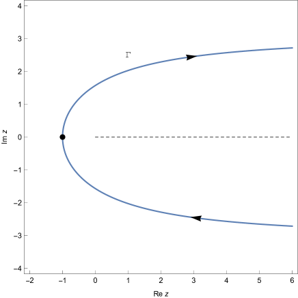
Figure 1: Integration contour $\Gamma$ for the partition function (12).

Then we rotate counterclockwise the path $\Gamma$ to the path $\Gamma_{\theta}$ illustrated in figure 2, while simultaneously change the determination of $W_{-}(z)$ to

$$W_{\theta}(z)=z-\log_{\theta}z,$$ (13)

where $\log_{\theta}z=\ln|z|+\rmi\arg z$ with $\theta\leq\arg z<\theta+2\pi$. With these integration contour $\Gamma_{\theta}$ and determination $W_{\theta}(z)$, the rotated integral converges in the half-plane $\theta-\pi/2<\arg g<\theta+\pi/2$, and that the rotated and unrotated integrals are equal in $\theta<\arg g<\pi/2$ and $\theta-\pi/2<\arg g<0$.

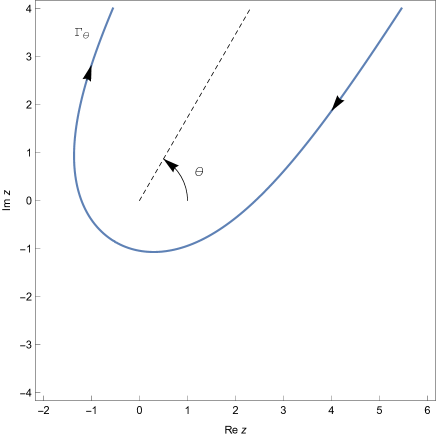
Figure 2: Rotated integration contour $\Gamma_{\theta}$ for the analytic continuation of the partition function (12).

Thus, setting $\theta=\pi$, we find that the analytic continuation $\mathcal{Z}_{n}(g)=Z_{n}^{({\rm cont})}(-g)$ for $g>0$ reads

$$\mathcal{Z}_{n}(g)=\frac{C_{n}(-g)}{(1-\rme^{-2\pi\rmi/g})^{n}}\frac{1}{n!}\left(\prod_{i=1}^{n}\int_{\Gamma_{\pi}}\rmd z_{i}\,\rme^{(z_{i}-\log_{\pi}z_{i})/g}\right)\Delta({\bf z})^{2}.$$ (14)

Finally we change variables $z_{i}\to-z_{i}$, and taking into account that $\log_{\pi}(-z)=\log_{0}z+\rmi\pi$ it follows that

$$\mathcal{Z}_{n}(g)=\frac{C_{n}(-g)(-1)^{n}\rme^{-\rmi n\frac{\pi}{g}}}{(1-\rme^{-2\pi\rmi/g})^{n}}\frac{1}{n!}\left(\prod_{i=1}^{n}\int_{\Gamma}\rmd z_{i}\rme^{-(z_{i}+\log z_{i})/g}\right)\Delta({\bf z})^{2},$$ (15)

or, equivalently,

$$\mathcal{Z}_{n}(g)=C_{n}(-g)(-2\rmi)^{-n}(\sin(\pi/g))^{-n}\,\mathcal{Z}^{(0)}_{n}(g),$$ (16)

where $\mathcal{Z}^{(0)}_{n}(g)$ is the holomorphic matrix integral [29]

$$\mathcal{Z}^{(0)}_{n}(g)=\frac{1}{n!}\left(\prod_{i=1}^{n}\int_{\Gamma}\rmd z_{i}\,\rme^{-W_{+}(z_{i})/g}\right)\Delta(\mathbf{z})^{2},$$ (17)

and

$$W_{+}(z)=z+\log z.$$ (18)

We stress that the partition function $\mathcal{Z}_{n}(g)$ given by equation (14) in effect defines the Penner model for negative values of the coupling constant. Note in particular the factorization into a prefactor (the first fraction) and the eigenvalue integral $\mathcal{Z}^{(0)}_{n}(g)$ studied in reference [29].

As a check of this analytic continuation process, we recall that using generalized Laguerre polynomials $L^{(-1/g)}_{n}(z/g)$ [30, 31] it was proved in reference [29] that $\mathcal{Z}^{(0)}_{n}(g)$ can be expressed in terms of the Barnes function as

$$\mathcal{Z}^{(0)}_{n}(g)=g^{n(n-\frac{1}{g})}(1-\rme^{-2\pi\rmi/g})^{n}\frac{G(1+n)G\left(1+n-\frac{1}{g}\right)}{G\left(1-\frac{1}{g}\right)}.$$ (19)

Hence, since

$$C_{n}(-g)=\frac{\rme^{-n/g}(-g)^{-n^{2}/2}}{(2\pi)^{n/2}G(1+n)},$$ (20)

we finally get

$$\mathcal{Z}_{n}(g)=\frac{(-\rme g)^{-n/g}(-g)^{n^{2}/2}}{(2\pi)^{n/2}}\frac{G(1+n-\frac{1}{g})}{G(1-\frac{1}{g})},\quad g>0,$$ (21)

which is the same expression obtained by replacing $g\to-g$ in equation (7).

Hereafter we will shorten the full qualification “Penner model with negative coupling constant” to simply “Penner model” when we refer to the model specified by the partition function $\mathcal{Z}_{n}(g)$.

3 The large-$n$ limit of the free energy

3.1 The large-$n$ limit with ’t Hooft sequences

Let us analyze the large-$n$ limit of the partition function $\mathcal{Z}_{n}(g)$ with ’t Hooft sequences $g_{n}=t/n$. From (21) and applying the reflection formula (69) to $\ln\left|G\left(1+n-1/g\right)\right|$ and to $\ln\left|G\left(1-1/g\right)\right|$ we have

$$\mathcal{F}_{n}(g_{n}) = -\frac{\ln|\mathcal{Z}_{n}(g_{n})|}{n^{2}}$$ (22)

$$= -\frac{1}{2n}\ln\left(\frac{\pi}{2}\right)+\left(\frac{1}{ng_{n}}-\frac{1}{2}\right)\ln g_{n}+\ln\left|\sin\left(\frac{\pi}{g_{n}}\right)\right|^{1/n}$$

$${}+\frac{1}{ng_{n}}-\frac{1}{n^{2}}\ln\left|G\left(1-n+\frac{1}{g_{n}}\right)\right|+\frac{1}{n^{2}}\ln\left|G\left(1+\frac{1}{g_{n}}\right)\right|.$$

Since $1+1/g_{n}>0$, the term $\ln|G(1+1/g_{n})|$ in (22) has a Stirling expansion of the type (67). However, the sign of the argument in $\ln|G(1-n+1/g_{n})|$ depends on the value of $t$. Indeed, for $0<t<1$ and large $n$ we have

$$\ln\Big{|}G\left(1-n+\frac{1}{g_{n}}\right)\Big{|}=\ln\Big{|}G\left(1+x\right)\Big{|},\quad x=n\left(\frac{1}{t}-1\right)\rightarrow+\infty,$$ (23)

so that this function has also a Stirling expansion of the type (67). However, for $1<t<\infty$ and large $n$ we have

$$\ln\Big{|}G\left(1-n+\frac{1}{g_{n}}\right)\Big{|}=\ln\Big{|}G\left(1-x\right)\Big{|},\quad x=n\left(1-\frac{1}{t}\right)\rightarrow+\infty,$$ (24)

and we have to use the expansion (Appendix A. The Barnes $G$ function) of Appendix A. Therefore, in this region the free energy can be decomposed into a sum of an oscillatory contribution and a perturbative contribution

$$\mathcal{F}_{n}(t)=\mathcal{F}^{(\rm osc)}_{n}(t)+\mathcal{F}^{(\rm per)}_{n}(t),$$ (25)

where

$$\mathcal{F}^{(\rm osc)}_{n}(t)=\left\{\begin{array}[]{ll}\ln\left|2\sin(\pi n/t)\right|^{1/n},&\mbox{for $0<t<1$,}\\ \frac{1}{t}\ln\left|2\sin(\pi n/t)\right|^{1/n}+\frac{1}{2\pi n^{2}}{\rm Cl}_{2}\left(2\pi n/t\right),&\mbox{for $1<t<\infty$,}\end{array}\right.$$ (26)

and in both cases, i.e., for $t\neq 1$, the perturbative contribution is

$$\mathcal{F}_{n}^{{\rm(per)}}(t) \approx -\left(\frac{(t-1)^{2}}{2t^{2}}\ln|1-t|-\frac{3}{4}+\frac{1}{2t}\right)+\frac{1}{12n^{2}}\ln|1-t|$$ (27)

$$- \sum_{k=2}^{\infty}\frac{B_{2k}}{2k(2k-2)}n^{-2k}t^{2k-2}\left((1-t)^{2-2k}-1\right),\quad n\rightarrow\infty.$$

The perturbative contribution $\mathcal{F}_{n}^{{\rm(per)}}(t)$ coincides with the standard large-$n$ expansion for the Penner model with negative coupling constant [22, 23]. Comparing the expression (27) with the topological expansion (72)–(74) of the Penner model with positive coupling constant, it is clear that $\mathcal{F}_{n}^{{\rm(per)}}(t)$ also represents a generating function for the virtual Euler characteristics. To the best of our knowledge, the oscillatory contribution $\mathcal{F}^{(\rm osc)}_{n}(t)$ has not been considered in the literature. Note also that the value $t=1$ is a critical value for both contributions.

3.2 The planar limit

The planar limit of the free energy

$$\mathcal{F}=\lim_{n\rightarrow\infty}\mathcal{F}_{n},$$ (28)

is not well-defined with the standard ’t Hooft sequences (9). Indeed, from the expression (26) of $\mathcal{F}^{(\rm osc)}_{n}(t)$ it is clear that the existence of $\mathcal{F}$ requires the existence of the limit $l$ defined in equation (11).

Thus, instead of restricting to sequences satisfying the ’t Hooft coupling, we use KM sequences. From equations (25)–(27) it follows that for $t\neq 1$

$$\mathcal{F}=\left\{\begin{array}[]{cc}\ln l-\frac{(t-1)^{2}}{2t^{2}}\ln|t-1|+\frac{3}{4}-\frac{1}{2t},&\mbox{for $0<t<1$,}\\ &\\ \frac{1}{t}\,\ln l-\frac{(t-1)^{2}}{2t^{2}}\ln|t-1|+\frac{3}{4}-\frac{1}{2t},&\mbox{for $1<t<\infty$.}\end{array}\right.$$ (29)

It is illustrative to clarify the origin of the different terms in equation (29) with respect to the factors in the equation (16). From equation (20) and taking into account that

$$\frac{1}{n^{2}}\ln|G(1+n)|=\frac{1}{2}\ln n-\frac{3}{4}+O(1/n),\quad n\rightarrow\infty,$$ (30)

it follows that

$$\mathcal{F}=\ln l+\frac{1}{t}+\frac{1}{2}\ln t+\frac{3}{4}+\mathcal{F}^{(0)},$$ (31)

where $\mathcal{F}^{(0)}$ is the planar free energy for $\mathcal{Z}^{(0)}_{n}$ [29]

$$\mathcal{F}^{(0)}=H(t-1)\left(\frac{1}{t}-1\right)\ln l-\frac{1}{2}\ln t+\frac{3}{2}\left(\frac{t-1}{t}\right)-\frac{(t-1)^{2}}{2t^{2}}\ln|t-1|,$$ (32)

where $H(x)$ is the Heaviside step function. It is now clear that the term $\ln l$ of $\mathcal{F}$ in the weak-coupling case comes only from the factor $|\sin(\pi/g)|^{-n}$ in (16), while the term $(\ln l)/t$ of $\mathcal{F}$ in the strong-coupling case is a result of the contributions from the two factors $|\sin(\pi/g)|^{-n}$ and $|\mathcal{Z}^{(0)}_{n}|$ in (16).

3.3 The phase space of the Penner model for negative values of the coupling constant

The $l$-dependence of the planar free energy means that from the point of view of KM sequences, the phase space of the Penner model in the planar limit is the set

$$\mathcal{P}=\{(t,l)\in\mathbb{R}^{2}\,|\,0<t<\infty,\;0\leq l\leq 1\}.$$ (33)

In this way KM sequences reveal a fine phase space structure (see figure 3), where both the weak- and strong-coupling phases depend on the additional parameter $l$. The points $(t,l)=(1,l)$ for $0<l<1$ represent first-order phase transitions

$$\mathcal{F}\Big{|}_{t=1-0}=\mathcal{F}\Big{|}_{t=1+0},\quad\frac{\partial\mathcal{F}}{\partial t}\Big{|}_{t=1-0}=\frac{\partial\mathcal{F}}{\partial t}\Big{|}_{t=1+0}+\ln l,$$ (34)

while the point $(t,l)=(1,1)$ represents a continuous phase transition in which $\mathcal{F}$ and $\partial\mathcal{F}/\partial t$ are continuous at $t=1$ but $\partial^{2}\mathcal{F}/\partial t^{2}$ diverges. Furthermore, the line $l=0$ represents a singular phase with infinite free energy.

It is possible to characterize wide classes of KM sequences for all $0<t<\infty$ and $0\leq l\leq 1$, as for example the one-parameter family

$$g_{n}=\frac{1}{[n/t]+c\,l^{n}},\quad c\neq 0,$$ (35)

where $[x]$ denotes the integer part of $x$. They also arise as subsequences of ’t Hooft sequences $g_{n}=t/n$. For example, given an irreducible fraction $t=p/q$ $(p>1)$, the subsequences $g_{np}$ and $g_{np+1}$ of the ’t Hooft sequence are KM sequences with $l=0$ and $l=1$, respectively. For irrational $t$ we have that the sequence $\{n/t\}$, where $\{x\}$ denotes the fractional part of $x$ is a dense subset of the interval $[0,1]$, so that all subsequences of the ’t Hooft sequence $g_{n}=t/n$ such that $\{k_{n}/t\}\rightarrow x$ for some $0<x<1$ are KM sequences with $l=1$. The value $l=1$ represents the generic case of KM sequences (see remark 1.3 in [28]).

A deeper understanding of the phase space of the Penner model is obtained from the analysis of the asymptotic eigenvalue (saddle point) distribution.

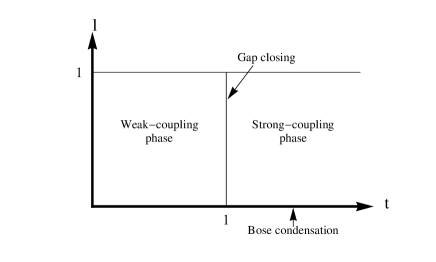
Figure 3: Phase space of the non-Hermitian Penner model with negative coupling constant for KM sequences.

4 Large-$n$ saddle points and Coulomb gas

The KM sequences originated in the theory of large-$n$ asymptotics of zeros of generalized Laguerre polynomials [27, 28]

$$L^{(\alpha)}_{n}(z)=\sum_{k=0}^{n}\left(\begin{array}[]{c}n+\alpha\\ n-k\end{array}\right)\frac{(-z)^{k}}{k!},\quad\alpha<0.$$ (36)

In [29] we showed how these zeros determine the saddle points of the holomorphic matrix integral $\mathcal{Z}^{(0)}_{n}(g)$ for KM sequences in the strong-coupling case. In order to describe the phase transitions at $t=1$, we will extend here the analysis of [29] by considering the weak-coupling case too.

4.1 Complex saddle points

The saddle point equations for $\mathcal{Z}^{(0)}_{n}(g)$ are

$$\frac{1}{g_{n}}\left(1+\frac{1}{z_{i}^{(n)}}\right)+\sum_{j\neq i}\frac{2}{z_{j}^{(n)}-z_{i}^{(n)}}=0,\quad i=1,\ldots,n,$$ (37)

and their solutions are given by [29]

$$z_{i}^{(n)}=g_{n}\,l^{(\alpha_{n},n)}_{i},\quad i=1,\ldots,n,$$ (38)

where $l^{(\alpha_{n},n)}_{i}$ are the zeros of the Laguerre polynomials $L^{(\alpha_{n})}_{n}(z)$ with

$$\alpha_{n}=-1-\frac{1}{g_{n}}.$$ (39)

Let us denote by $\rho(z)$ the asymptotic eigenvalue (saddle point) distribution for the Penner model and by $\rho_{L}(z)$ the asymptotic zero distribution of the scaled Laguerre polynomials $L^{(\alpha_{n})}_{n}(nz)$. The form of $\rho_{L}(z)$ has been completely characterized in the large-$n$ limit

$$n\rightarrow\infty,\quad\frac{\alpha_{n}}{n}\rightarrow A=\mbox{fixed},$$ (40)

for all real values of $A$ in references [27, 28, 32, 33]. Using (38) and (39) we can immediately translate the properties of $\rho_{L}(z)$ into properties of $\rho(z)$, since

$$t=-\frac{1}{A},\quad\rho(z)=\frac{1}{t}\rho_{L}\left(\frac{z}{t}\right).$$ (41)

It turns out that the zeros of $L^{(\alpha_{n})}_{n}(nz)$ cluster along certain curves $\gamma_{L}$ in the complex plane. More concretely, if we denote

$$a_{\pm}=A+2\pm 2\sqrt{A+1},$$ (42)

1. For $-\infty<A<-1$ (the weak-coupling region $0<t<1$) the curve $\gamma_{L}$ is a simple open arc with endpoints $a_{-}$ and $a_{+}=\overline{a}_{-}$ symmetric with respect to $\mathbb{R}$, which as $A\rightarrow-1$ closes and becomes the Szegő curve

   $$|z\,\rme^{1-z}|=1,\quad|z|\leq 1.$$ (43)

   This process is shown in figure 4. The corresponding zero density is

   $$\rho_{L}(z)=\frac{1}{2\pi}\left|\frac{\sqrt{(z-a_{-})(z-a_{+})}}{z}\right|.$$ (44)

2. For $-1<A<0$ (the strong-coupling region $1<t<\infty$), and if the limit

   $$l=\lim_{n\rightarrow\infty}|\sin(\alpha_{n}\pi)|^{1/n}=\lim_{n\rightarrow\infty}|\sin(\pi/g_{n})|^{1/n},$$ (45)

   exists, then $\gamma_{L}$ is of the form

   $$\gamma_{L}=C_{l}\cup[a_{-},a_{+}],$$ (46)

   where

   1. For $l\neq 0$ the curve $C_{l}\subset\mathbb{C}\setminus(\{0\}\cup[a_{-},+\infty))$ is a simple closed curve encircling $0$ once, which is determined by the implicit equation

      $${\rm Re}\,\int_{a_{-}}^{z}\frac{\sqrt{(z^{\prime}-a_{-})(z^{\prime}-a_{+})}}{z^{\prime}}{\rm d}z^{\prime}=-\log l.$$ (47)

      The corresponding zero density is

      $$\rho_{L}(z)=\frac{1}{2\pi}\left|\frac{\sqrt{(z-a_{-})(z-a_{+})}}{z}\right|.$$ (48)

   2. For $l=0$

      $$\gamma_{L}=\{0\}\cup[a_{-},a_{+}],$$ (49)

      and the zero density is

      $$\rho_{L}(z)=A\,\delta(z)+\frac{1}{2\pi}\left|\frac{\sqrt{(x-a_{-})(x-a_{+})}}{x}\right|\chi_{[a_{-},a_{+}]},$$ (50)

   where $\chi_{[a_{-},a_{+}]}$ is the characteristic function of the real interval $[a_{-},a_{+}]$. The filling fraction of the zero density on $C_{l}$ is equal to $|A|$. The value $l=1$ is the generic case (see remark 1.3 in reference [28]), and it follows from equation (47) that it is the only situation in which the loop $C_{l}$ and the interval $[a_{-},a_{+}]$ intersect (at the point $a_{-}$). It should be noticed that the form of $\gamma_{L}$ depends not only on the value of $A$ but also on $l$.

4.2 Coulomb gas, gap closing, eigenvalue tunneling and Bose condensation

In this section we use the electrostatic interpretation wherein the eigenvalue density $\rho(z)$ is thought of as a unit normalized positive charge density for a Coulomb gas in the external electrostatic potential

$$V(z)=x+\ln|z|,\quad(x=\mathop{\rm Re}\nolimits z).$$ (51)

The electrostatic energy of the Coulomb gas,

$$\mathcal{E}(t)=\frac{1}{t}\int_{\gamma}V(z)\rho(z)|{\rmd}z|-\int_{\gamma}|\rmd z|\int_{\gamma}|\rmd z^{\prime}|\ln|z-z^{\prime}|\rho(z)\rho(z^{\prime}),$$ (52)

is given [29] by

$$\mathcal{E}(t)=-\frac{1}{2}\ln t-\frac{(t-1)^{2}}{2t^{2}}\ln|t-1|+\frac{3}{2}\left(1-\frac{1}{t}\right).$$ (53)

We remark that $\mathcal{E}(t)$ is independent of $l$.

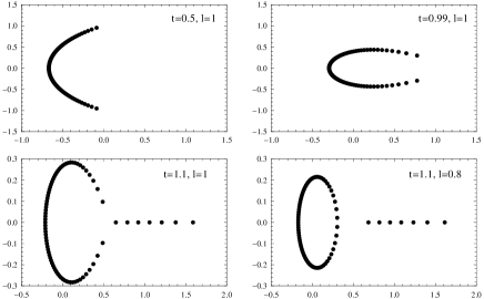
Figure 4: Eigenvalue distribution in the gap-closing phase transition for $n=80$.

The form of the support of $\rho(z)$ is independent of $l$ in the weak-coupling phase, but it depends on $l$ in the strong-coupling phase. Thus for $1<t<\infty$ the support of $\rho(z)$ consists of two pieces: an $l$-dependent closed loop $\gamma_{1}$ around the origin with filling fraction $1/t$, and an $l$-independent interval $\gamma_{2}=[ta_{-},ta_{+}]$ on the positive real axis with filling fraction $1-1/t$.

The points of the weak-coupling phase are electrostatic stable equilibrium configurations of $\rho(z)$. However, points of the strong-coupling phase represent stable electrostatic equilibrium configurations only for $l=1$ [29]. Indeed, for strong coupling the effective potential of the charge distribution corresponding to $\rho(z)$

$$V_{\rm eff}(z)=V(z)-2t\int_{\gamma}\ln|z-z^{\prime}|\rho(z^{\prime})|\rmd z^{\prime}|,$$ (54)

is constant on the two pieces of the support of $\gamma$ [29], but with values

$$V_{\rm eff}\big{|}_{\gamma_{1}}=-t\ln l+V_{\rm eff}\big{|}_{\gamma_{2}},\quad V_{\rm eff}\big{|}_{\gamma_{2}}=(2t-1)-t\ln t-(t-1)\ln(t-1),$$ (55)

which coincide for $l=1$ only.

Finally, note the following two types of phase transitions:

1. In the weak-coupling phase the limit $t\rightarrow 1$ and constant $l\neq 0$ represents a gap-closing (confining) transition in which the open arc formed by the support of $\rho(z)$ closes and becomes the Szegő curve (figure 4). In the strong-coupling phase this limit represents a gap-opening (deconfining) transition mediated by an eigenvalue tunneling process in which the charge $1-1/t$ located on the interval $\gamma_{2}$ tunnels to the higher-potential points of the loop $\gamma_{1}$.

2. As $l\rightarrow 0$ from the strong-coupling phase with constant $t$ the loop $\gamma_{1}$ of the support of $\rho(z)$ shrinks to the point $z=0$ forming a condensate of charge $1/t$ (figure 5). This represents a process of Bose condensation in which the electrostatic energy $\mathcal{E}$ (53) remains finite and constant. However, the planar free energy diverges ($\mathcal{F}\rightarrow-\infty$) as a consequence of the contribution to $\mathcal{F}$ of the oscillatory factor in (16).

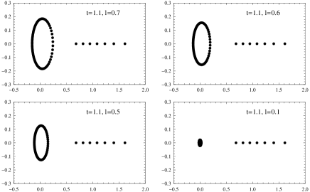
Figure 5: Eigenvalue distribution in Bose condensation for $n=80$.

5 Outlook

There are several relevant non-Hermitian matrix models which have a phase space in the large-$n$ limit with properties similar to the Penner model with negative coupling constant. We will briefly mention some examples.

Multi-Penner models of the form

$$W(z)=-\sum_{i=1}^{k}\mu_{i}\log(z-q_{i}),$$ (56)

have been introduced to characterize the correlation functions of the $d=2$ conformal $A_{1}$ Toda field theory [14, 34]. The simplest case is the double Penner model [14]

$$W(z)=-\mu_{+}\log(1-z)-\mu_{-}\log(z+1),$$ (57)

which is connected to the theory of Jacobi polynomials

$$P^{(\alpha,\beta)}_{n}(z)=2^{-n}\sum_{k=0}^{n}\left(\begin{array}[]{c}n+\alpha\\ n-k\end{array}\right)\left(\begin{array}[]{c}n+\beta\\ k\end{array}\right)(z-1)^{k}(z+1)^{n-k},$$ (58)

with

$$\alpha=\frac{\mu_{+}}{g},\quad\beta=\frac{\mu_{-}}{g}.$$ (59)

The Hermitian matrix model corresponds to the classical Jacobi polynomials with $\alpha,\beta>-1$. Its large-$n$ limit with ’t Hooft sequences is well defined, and the eigenvalue distribution is determined by the asymptotic zero distribution of the Jacobi polynomials on the real interval $[-1,1]$. However, there are non-classical cases for which the existence of the planar limit requires a special formulation based on KM sequences [35]. For example, if we take a large-$n$ limit with sequences $ng_{n}\rightarrow t>0$ such that

$$n\rightarrow\infty,\quad\frac{\alpha_{n}}{n}\rightarrow A=\frac{\mu_{+}}{t},\quad\frac{\beta_{n}}{n}\rightarrow B=\frac{\mu_{-}}{t},$$ (60)

where

$$-1<A<0<B,$$ (61)

or, equivalently,

$$\mu_{+}<0,\quad\mu_{-}>0,\quad t>|\mu_{+}|.$$ (62)

Then the existence of a well-defined asymptotic zero distribution requires the existence of the limit [35]

$$l=\lim_{n\rightarrow\infty}|\sin(\pi An)|^{1/n}.$$ (63)

The corresponding zero distribution of non-classical Jacobi polynomials exhibits properties like gap-closing processes [35], similar to the generalized Laguerre polynomials. Therefore it would be interesting to analyze the non-Hermitian version of the double Penner model following the scheme used in the present paper for the Penner model.

Families of Laguerre polynomials also appear in certain matrix models used to study the low-energy limit in Quantum Chromodynamics, e.g., the chiral Gaussian Unitary matrix model (also called the Wishart-Laguerre ensemble) [36, 37]

$$Z_{n}^{(N_{f},\nu)}=\frac{1}{n!}\left(\prod_{i=1}^{n}\int_{0}^{\infty}\rmd x_{i}\,x_{i}^{\nu}\rme^{-x_{i}}\prod_{f=1}^{N_{f}}(x_{i}+m_{f}^{2})\right)\Delta(\mathbf{x})^{2},$$ (64)

where $N_{f}>0$ is the number of fermionic quark flavors, $m_{f}$ $(f=1,\ldots,N_{f})$ are the corresponding masses, and $\nu\geq 0$ is the topological charge of the physical sector under consideration.

This partition function can be determined in terms of Laguerre polynomials (see [37] and the references therein). For example, it is clear that the reduced case with $m_{f}=0$ for all $f$ gives

$$\mathcal{Z}_{n}^{(N_{f},\nu)}=\frac{1}{n!}\left(\prod_{i=1}^{n}\int_{0}^{\infty}\rmd x_{i}\,x_{i}^{\nu+N_{f}}\rme^{-x_{i}}\right)\Delta(\mathbf{x})^{2},$$ (65)

which is directly associated to the family of Laguerre polynomials $L^{(\nu+N_{f})}_{n}(x)$. Consequently, non-Hermitian versions of (65), like those arising from (64) with bosonic quarks ($N_{f}<0$) [38], will involve families of generalized Laguerre polynomials and may exhibit non-perturbative effects similar to the Penner model with negative coupling constant.

Appendix A. The Barnes $G$ function

This Appendix collects the properties that we need about the Barnes $G$ function [39, 40, 41]. The Barnes $G$ function is the entire function defined by the canonical product

$$G(1+z)=(2\pi)^{z/2}\rme^{-\frac{1}{2}(z+z^{2}(1+\gamma))}\prod_{k=1}^{\infty}\left(1+\frac{z}{k}\right)^{k}\rme^{-z+z^{2}/2k}.$$ (66)

The Stirling-like asymptotic expansion of $G(1+z)$ for $z=x$ positive and large is

$$\ln G(1+x) \sim \frac{1}{2}x^{2}\ln x-\frac{3}{4}x^{2}+\frac{x}{2}\ln(2\pi)-\frac{1}{12}\ln x$$ (67)

$${}+\zeta^{\prime}(-1)+\widetilde{\varphi}(x),\qquad\mathrm{as}\quad x\to\infty,$$

where $\widetilde{\varphi}(x)$ is the asymptotic negative power series

$$\widetilde{\varphi}(x)=\sum_{m=2}^{\infty}\frac{B_{2m}}{2m(2m-2)}\frac{1}{x^{2m-2}}.$$ (68)

Incidentally, we mention here that the asymptotic series $\widetilde{\varphi}(x)$ provides the connection between Penner models and string theory [42], because $\widetilde{\varphi}(\rmi\mu)$ determines the genus expansion $\widetilde{F}_{c=1}(\mu)$ of the free energy of the $c=1$ string theory at the self-dual radius. The sector of validity of equation (67) is often quoted as $-\pi<\arg z<\pi$ or, more precisely, $|\arg z|\leq\pi-\delta$ with $\delta>0$ (see equation 5.17.5 in [40]). We want to emphasize that the expansion (67) is asymptotic in this sector only in the sense of Poincaré.

To evaluate the $G$ function for large negative real values of the argument we use the reflection formula (see equation (6) of [41]) to obtain

$$\ln|G(1-x)|=\ln G(1+x)+x\ln\left|\frac{\sin(\pi x)}{\pi}\right|+\frac{1}{2\pi}\mathop{\rm Cl}_{2}\nolimits(2\pi x),$$ (69)

where $\mathrm{Cl}_{2}(x)$ is the Clausen function

$$\mathop{\rm Cl}_{2}\nolimits(x)=-\int_{0}^{x}\ln\left|2\sin\frac{\tau}{2}\right|\rmd\tau=\sum_{m=1}^{\infty}\frac{\sin(mx)}{m^{2}}.$$ (70)

Note that equation (6) in [41] is limited to $0<x<1$.

Thus, from (67) and (69) we obtain

$$\ln|G(1-x)|-x\ln\left|\frac{\sin(\pi x)}{\pi}\right|-\frac{1}{2\pi}\mathop{\rm Cl}_{2}\nolimits(2\pi x)\sim$$

$$\qquad\frac{1}{2}x^{2}\ln x-\frac{3}{4}x^{2}+\frac{x}{2}\ln(2\pi)-\frac{1}{12}\ln x+\zeta^{\prime}(-1)+\widetilde{\varphi}(x),$$

$$\qquad\qquad x\rightarrow\infty.$$ (71)

The second term in the left-hand side of (Appendix A. The Barnes $G$ function) cancels the singularities of $\ln|G(1-x)|$ at positive integer values of $x$, and therefore the left-hand side of (Appendix A. The Barnes $G$ function) has a well-defined asymptotic expansion. However, in order to have a well-defined large-$n$ free energy of the Penner model with negative coupling constant, we need to control the behavior of $\ln|G(1-x)|$ as $x$ becomes large. Obviously the terms $x\ln\left|\sin(\pi x)/\pi\right|$ and $\mathop{\rm Cl}_{2}\nolimits(2\pi x)/2\pi$ in (Appendix A. The Barnes $G$ function) are the origin of the $\mathcal{F}^{(\rm osc)}$ in (26) and $l$-dependent contributions in (29) arising in the planar free energy of the Penner model. Therefore we have to restrict the way in which the coupling constant $g$ tends to zero (and consequently $x$ to infinity) in such a way that these terms give well-defined contributions to the planar limit. This is the ultimate reason for requiring the existence of the limit (11).

Appendix B. The topological expansion of the Penner model with positive coupling constant

The large $n$ expansion of the Penner model with positive coupling constants for ’t Hooft sequences can be readily obtained from equations (7) and (67),

$$F_{n}(t) = -\frac{\ln|Z_{n}(g)|}{n^{2}}$$ (72)

$$\approx -\left(\frac{(t+1)^{2}}{2t^{2}}\ln(1+t)-\frac{3}{4}-\frac{1}{2t}\right)+\frac{1}{12n^{2}}\ln(1+t)$$

$${}-\sum_{k=2}^{\infty}\frac{B_{2k}}{2k(2k-2)}n^{-2k}t^{2k-2}\left((1+t)^{2-2k}-1\right)$$

$$= -\sum_{k\geq 0}^{\infty}n^{-2k}\sum_{s>0,2-2k-s<0}\frac{(-1)^{s}(2k+s-3)!(2k-1)}{(2k)!s!}B_{2k}\,t^{2k+s-2}$$

$$\quad n\rightarrow\infty.$$

Alternatively, the standard perturbative method applied to (7) leads to a topological expansion of the form [19, 24]

$$F_{n}(t)\approx-\sum_{k\geq 0}^{\infty}n^{-2k}\sum_{s>0,2-2k-s<0}\chi_{k,s}\,t^{2k+s-2},$$ (73)

where $\chi_{k,s}$ is the virtual Euler characteristic of the space of Riemann surfaces of genus $k$ with a finite number $s$ of punctures. Then equations (72) and (73) imply [19]

$$\chi_{k,s}=\frac{(-1)^{s}(2k+s-3)!(2k-1)}{(2k)!s!}B_{2k}.$$ (74)

References

References

- [1] Hollowood T J, Kumar S P and Myers J C 2011 J. High Energy Phys. 11 138
- [2] Jain S, Minwalla S, Sharma T, Takimi T, Wadia S R and Yokoyama S 2013 J. High Energy Phys. 09 009
- [3] Hollowood T J and Kumar S P 2015 J. High Energy Phys. 12 016
- [4] Buividovich P V, Dunne G V and Valgushev S N 2016 Phys. Rev. Lett. 116 132001
- [5] Álvarez G, Martínez Alonso L and Medina E 2016 Phys. Rev. D 94 105010
- [6] David F 1991 Nuc. Phys. B 348 507–524
- [7] David F 1993 Phys. Lett. B 302 403–410
- [8] Bonnet G, David F and Eynard B 2000 J. Phys. A: Math. Gen. 33 6739–6768
- [9] Mariño M, Schiappa R and Weiss M 2008 Commun. Number Theory Phys. 2 349–419
- [10] Eynard B 2009 J. High Energy Phys. 0903 03
- [11] Mariño M, Schiappa R and Weiss M 2009 J. Math. Phys. 50 052301
- [12] Mariño M 2008 J. High Energy Phys. 12 114
- [13] Schiappa R and Vaz R 2014 Commun. Math. Phys. 330 655
- [14] Schiappa R and Wyllard N 2010 J. Math. Phys. 51 0802304
- [15] Pasquetti S and Schiappa R 2010 Ann. Henri Poincaré 11 351–431
- [16] Mariño M 2014 Fortschr. Phys. 62 455–540
- [17] Gross D and Witten E 1980 Phys. Rev. D 21 446–453
- [18] Wadia S R 1980 Phys. Lett. B 93 403–410
- [19] Penner R C 1988 J. Diff. Geom. 27 35–53
- [20] Distler J and Vafa C 1991 The Penner model and string theory Random surfaces and quantum gravity (NATO Adv. Sci. Inst. Ser. B Phys. vol 262) (New York: Plenum) pp 243–253
- [21] Distler J and Vafa C 1991 Mod. Phys. Lett. A 6 259–270
- [22] Chair N and Panda S 1991 Phys. Lett. B 272 230–238
- [23] Matsuo Y 2006 Nuc. Phys. B 740 222–242
- [24] Mulase M 1998 Lectures on the asymptotic expansion of a hermitian matrix integral arXiv:math-ph/9811023
- [25] Deo N 2002 Phys. Rev. E 65 056115
- [26] Álvarez G, Martínez Alonso L and Medina E 2014 J. Phys. A: Math. and Theor. 47 315205
- [27] Kuijlaars A B J and McLaughlin K T R 2001 Comp. Methods and Function Theory 1 205–233
- [28] Kuijlaars A B J and McLaughlin K T R 2004 Constructive Approximation 20 497–523
- [29] Álvarez G, Martínez Alonso L and Medina E 2015 Ann. Phys. 361 440–460
- [30] Bessis D, Itzykson C and Zuber J B 1980 Adv. in Appl. Math. 1 109–157
- [31] Di Francesco P, Ginsparg P and Zinn-Justin J 1995 Phys. Rep. 254 1–133
- [32] Martínez-Finkelshtein A, Martínez-González P and Orive R 2001 J. Comp. and Appl. Math. 133 477–487
- [33] Díaz Mendoza C and Orive R 2011 J. Math. Anal. Appl. 379 305–315
- [34] Dijkgraaf R and Vafa C Toda theories, matrix models, topological strings, and gauge systems arXiv:0909.2453
- [35] Martínez-Finkelshtein A and Orive R 2005 J. Approx. Theory 134 137–170
- [36] Verbaarschot J J M 2006 QCD, chiral random matrix theory and integrability Applications of random matrices in physics (NATO Sci. Ser. II Math. Phys. Chem. vol 221) (Dordrecht: Springer) pp 163–217
- [37] Akemann G Random matrix theory and quantum chromodynamics arXiv:1603.06011
- [38] Splittorff K and Verbaarschot J J M 2006 Nuc. Phys. B 757 259–279
- [39] Barnes E W 1900 Quart. J. Pure Appl. Math. 31 264–314
- [40] Olver F W J, Lozier D W, Boisvert R F and Clark C W 2010 NIST Handbook of Mathematical Functions (Cambridge University Press)
- [41] Adamchik V S 2001 On the Barnes function Proceedings of the 2001 International Symposium on Symbolic and Algebraic Computation (New York: ACM) pp 15–20
- [42] Gross D J and Klebanov I R 1990 Nuc. Phys. B 344 475–498