Ordering of hard rectangles in strong confinement

Abstract

Using transfer operator and fundamental measure theories, we examine the structural and thermodynamic properties of hard rectangles confined between two parallel hard walls. The side lengths of the rectangle ($L$ and $D$, $L>D$) and the pore width ($H$) are chosen such that maximum two layers are allowed to form in planar order ($L$ is parallel to the wall), while only one in homeotropic order ($D$ is parallel to the wall). We observe three different structures: (i) a low density fluid phase with parallel alignment to the wall, (ii) an intermediate and high density fluid phase with two layers and planar ordering and (iii) a dense single fluid layer with homeotropic ordering. The appearance of these phases and the change in the ordering direction with density is a consequence of the varying close packing structures with $L$ and $H$. Interestingly, even three different structures can be observed with increasing density if $L$ is close to $H$.

I Introduction

The properties of molecular and colloidal systems can be altered substantially in restricted geometries such as slit-like pores, cylindrical tubes and spherical cavities. Even the simple hard sphere system confined between two parallel hard walls exhibits rich phase behaviour with changing the wall separation 1 . Due to the commensuration effect between the size of the sphere and the wall separation several intermediate (e.g. prism and rhombic phases) and crystalline structures with layers of square and triangle symmetries can be generated 2 . However, the phase behaviour of non-spherical hard bodies is even richer both in bulk and confinement as several liquid crystalline structures (e.g. nematic and smectic A), director distortion and domain walls may emerge due to the orientation dependence of particle-particle and wall-particle interactions. The ordering of hard rods between two planar hard walls is versatile as planar ordering and surface induced biaxial order may emerge in the vicinity of walls. As hard walls promote the orientational ordering, the isotropic phase may be suppressed and the isotropic-nematic transition (capillary nematization) terminates at a critical point with decreasing wall separation 3 ; 4 ; 5 ; 6 ; 7 . In addition to this the nematic-smectic A transition can be also suppressed and even layering transitions between periodic structures with $n$ and $n+1$ layers can be induced 8 ; 9 .

The system of two-dimensional (2D) hard objects, which can be realized by strong confinement of three-dimensional colloidal particles into a plane, can also exhibit wealthy phase behaviour in bulk and confinement. Among these the monolayer of square and rectangle-shaped hard particles has been studied extensively with simulation 10 ; 11 ; 12 , theory 13 ; 14 ; 15 ; 16 ; 17 ; 18 ; 19 and experiment 20 ; 21 ; 22 ; 23 ; 24 ; 25 . Interestingly, a tetratic phase of four-fold symmetry can be observed both in hard square 10 and weakly elongated hard rectangle systems 11 , while a nematic phase of two-fold symmetry can be stabilized in the system of elongated hard rectangles 13 . Several studies are devoted to the effect of confinement on the phase behaviour of hard squares and rectangles. In spherical and square cavities the nature of wall induced defective structures (e.g. topology of the defects, domain formation) are examined by density functional theories 26 ; 27 ; 28 ; 29 and Monte Carlo simulations 29 ; 30 ; 31 ; 32 . In slit pores the capillary nematisation and layering transitions are observed for large shape anisotropies with walls favouring homeotropic anchoring 32 . In the case of hard walls, planar ordering and increased nematic ordering can be seen with respect to isotropic and tetratic order 33 ; 34 .

Here we study the system of hard rectangles in a very narrow slit-like pore and search for the possibility of surface ordering, the formation of different structures and structural transitions. With the help of the transfer operator method (TOM) we obtain exact results for the thermodynamic quantities (e.g. density, heat capacity, vertical or normal pressure), while the fundamental measure density functional theory (FMT) is applied to get further information about the structure of observed phases. As the TOM of classical fluids is originally devised for one dimensional fluids 35 ; 36 ; 37 , we extend the method for confinements such that a maximum of two layers can form in planar ordering (particles’ long axes are parallel to the wall) or only one layer can accommodate within the pore in homeotropic ordering (particles’ long axes are perpendicular to the wall). We show that the structure of the fluid can be manipulated by the external longitudinal force, the particle’s shape anisotropy and the width of the pore. The low density (small external force) structure is always dominated by planar ordering, while the high density (large external force) structures can exhibit both planar and homeotropic ordering with one or two fluid layers. It may happen that three different fluid structures emerge upon compression of the system at some particular shape anisotropy and pore-width. However, our results clearly show that the changes in orientational and layering properties do not result in a true phase transition, but they correspond to structural transitions with marked peaks in heat capacity and compressibility.

II Transfer operator method of confined hard rectangles

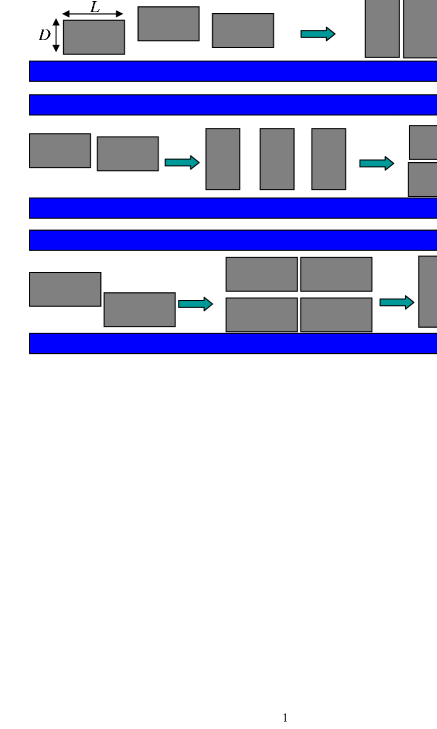
Figure 1: Possible phases and phase sequences of hard rectangles with increasing horizontal pressure ($P_{x}$) in a narrow hard channel, where $H$ is the width of the channel and $L$ ($D$) is the length (width) of the rectangles. At low pressures (densities) a fluid phase with one layer forms, where the particles align along the horizontal axis ($x$). This phase is denoted as FH1. At intermediate and high pressures (densities) either a single fluid layer with orientations along the vertical direction ($y$) or a fluid with two layers and horizontal order can be observed. These phases are referred to as FV and FH2, respectively. The upper panel shows a FH1-FV structural transition, while FH1-FV-FH2 and FH1-FH2-FV phase sequences can be seen in the middle and lower panels.

Here we consider a system of $N$ hard rectangles of side lengths $L$ and $D$ in a narrow hard channel with pore width $H$ at a given external force acting along the channel. The schematic of the channel and the possible structures of the rectangles are shown in Fig. 1. The Cartesian coordinate system is chosen to be in the middle of the pore, where $x$ and $y$ axes are along the horizontal and vertical directions, respectively. The external force ($f_{x}$), which sets the density of the rectangles, is pointing along the $x$ axis. To get exact results for this system, we restrict our study to the following conditions for the pore width, molecular dimensions and orientations. The allowed ranges of $L$ and $H$ are given by $D<L<3D$ and $L<H<\min\{L+D,3D\}$. Moreover, only horizontal and vertical orientations are allowed for the rectangles (restricted orientation model). In the horizontal state ($h$), the long axis of the particle is parallel to the confining walls, while the short axis of the particle is along the $x$ axis in the vertical state ($v$). These conditions guarantee that only particles being in $h$ states can pass each other, while there is no room for passage for $v$ state particles in the presence of $h$ or $v$ state particle. Therefore one or two layers can form in the horizontal state for $H>2D$, while only one in the vertical one (see Fig. 1). We now extend the transfer operator method for rotating rectangles, which was developed for parallel hard squares 38 . To do this, we start with the configurational part of the isobaric partition function of second neighbor interacting systems, which can be written as

$$Z= \int_{0}^{\infty}dL_{x}e^{-\beta f_{x}L_{x}}\times$$

$$\int\left(\prod_{i=1}^{N}dq_{i}\right)e^{-\beta\sum_{j=1}^{N}[u(q_{j},q_{j+1})+u(q_{j},q_{j+2})]},$$ (1)

where $\beta=1/k_{B}T$ is the inverse temperature, $L_{x}$ is the length of the pore, $q_{i}=(x_{i},y_{i},\varphi_{i})$ is a notation of the position and orientation of particle $i$ and $u(q_{i},q_{j})$ is the pair potential between particles $i$ and $j$. Note that $1/N!$ is missing, because we tacitly assumed that $0<x_{1}<x_{2}<\cdots<x_{N}<L_{x}$. We also employ the periodic boundary condition, which means that $q_{N+1}=q_{1}$ and $q_{N+2}=q_{2}$. The ranges of the integrals for the $y$ positions in Eq. (1) are $-(H-\sigma(\varphi_{i}))/2<y_{i}<(H-\sigma(\varphi_{i}))/2$. In our two-state model the orientation can be either horizontal or vertical, i.e. $\varphi_{i}=\{h,v\}$, and the vertical length of the particle is given by $\sigma(h)=D$ and $\sigma(v)=L$. Furthermore, the integral $\int d\varphi$ which is included in the $\int dq$ notation, is understood as a sum, $\sum_{\varphi\in\{h,v\}}$. Two like ($h-h$ and $v-v$) and one unlike ($v-h$) hard body interactions can be identified between $i$ and $j$ particles, which are given by

$$u[(x,y,v),(x^{\prime},y^{\prime},v)] =\left\{\begin{matrix}\infty&\text{if}\ |x-x^{\prime}|<D\\ 0&\text{otherwise}\end{matrix}\right.,$$ (2a)

$$u[(x,y,h),(x^{\prime},y^{\prime},h)] =\left\{\begin{matrix}\infty&\text{if}\ |x-x^{\prime}|<L\\ &\text{and}\ |y-y^{\prime}|<D\\ 0&\text{otherwise}\end{matrix}\right.,$$ (2b)

$$u[(x,y,h),(x^{\prime},y^{\prime},h)] =\left\{\begin{matrix}\infty&\text{if}\ |x-x^{\prime}|<\frac{L+D}{2}\\ 0&\text{otherwise}\end{matrix}\right..$$ (2c)

Note that only the $h-h$ pair potential depends on the vertical positions, while the other two are the same for any $y$ and $y^{\prime}$ positions. This is due to the geometrical conditions, which allow only the horizontal particles to form two layers in the pore. After substitution of Eqs. (2a)-(2c) into Eq. (1) one can realize that the integrations in horizontal variables ($x_{i}$) cannot be achieved, i.e. the traditional transfer operator method cannot be applied for this model. However, on the basis of our previous study for parallel hard squares 38 , it is feasible to work out a dimer-approach, where the two neighboring particles are considered as a dimer particle. If $N$ is an even number, i.e. we have $N/2$ dimers, the transfer operator method can be applied for the dimers, because as we show below the integrals in the dimer-dimer horizontal distances can be performed analytically. In the dimer-approach we introduce new notations. First of all, we label the dimers by capital letters to emphasize that the values of these indices are running up to $N/2$. Moreover, we introduce new variables instead of the original $x_{i}$ coordinates of the particles: $\hat{x}_{I}$ is the horizontal distance between the particles’ centers of a dimer $I$, and $X_{I,J}$ is the horizontal distance between the centers of mass of dimers $I$ and $J$. For the sake of simplicity we introduce $Q_{I}=(\hat{x}_{I},y_{I,1},y_{I,2},\varphi_{I,1},\varphi_{I,2})$ for the inner coordinates of dimer $I$, where $y_{I,n}$ and $\varphi_{I,n}$ (here $n=1,2$) are only new notations for the $y$ and $\varphi$ coordinates of the $2(I-1)+n$-th particle, which is the $n$-th member of the dimer $I$. At this point it is worth changing from the molecular coordinates to inner and relative neighboring ones ($Q_{I}$ and $X_{I,I+1}$) in Eq. (1) as follows $dL_{x}\prod_{i=1}^{N}dq_{i}\to dx_{1}\prod_{I=1}^{N/2}dQ_{I}dX_{I,I+1}$ . With the new variables there is no need for $L_{x}$ any more, as $L_{x}=\sum_{I=1}^{N/2}X_{I,I+1}$. However, the hard body exclusion sets the range of the inner variable $\hat{x}_{I}$ in Eq. (1) as follows: $\hat{x}_{I}>\sigma_{I,1;I,2}$, where $\sigma_{I,1;I,2}$ is the horizontal contact distance between the first and second particles of the dimer $I$. One can write the horizontal contact distance generally between particles $i$ and $j$ as

$$\sigma_{i;j}=\left\{\begin{array}[]{ccl}0,&\text{if}&\varphi_{i}=\varphi_{j}=h\text{ and }|y_{i}-y_{j}|>D\\ L,&\text{if}&\varphi_{i}=\varphi_{j}=h\text{ and }|y_{i}-y_{j}|<D\\ D,&\text{if}&\varphi_{i}=\varphi_{j}=v\\ \frac{L+D}{2},&\text{if}&\varphi_{i}\neq\varphi_{j}\end{array}\right.$$ (7)

therefore the horizontal contact distance between particles $n$ and $m$ of dimers $I$ and $J$ is

$$\sigma_{I,n;J,m}=\sigma_{2(I-1)+n,2(J-1)+m}.$$ (8)

Note that Eq. 7 can be obtained easily from the pair interactions, see Eqs. (2). The lower bound of the neighboring dimer distance ($X_{i,i+1}$) is constrained by prohibiting the overlap between dimers. Therefore one can get that $\sigma_{I,I+1}<X_{I,I+1}$ in the partition function, where $\sigma_{I,I+1}$ is the horizontal contact distance between two neighboring dimers. As first-first, second- first and second-second contacts may occur between particles of two neighboring dimers, the contact distance can be written as the maximum of the three possible values, as follows:

$$\sigma_{I,I+1}\equiv\max\left\{\sigma_{I,2;I+1,1}+\frac{\hat{x}_{I}+\hat{x}_{I+1}}{2},\right.$$

$$\left.\sigma_{I,1;I+1,1}+\frac{-\hat{x}_{I}+\hat{x}_{I+1}}{2},\right.$$

$$\left.\sigma_{I,2;I+1,2}+\frac{\hat{x}_{I}-\hat{x}_{I+1}}{2}\right\}.$$ (9)

As can be seen from Eq. (7), $\sigma_{I,I+1}$ depends on the variables $Q_{I}$ and $Q_{I+1}$. Using the new inner and outer variables one can rewrite Eq. 1 as follows

$$Z = \int\left(\prod_{I=1}^{N/2}dQ_{I}dX_{I,I+1}\right)e^{-P\sum_{J=1}^{N/2}X_{J,J+1}}$$

$$= \int\left(\prod_{I=1}^{N/2}dQ_{I}\right)\prod_{J=1}^{N/2}\left(\int_{\sigma_{J,J+1}}^{\infty}dX_{J,J+1}e^{-PX_{J,J+1}}\right),$$

where $P=\beta f_{x}$. The benefit of this form of $Z$ is that $N/2$ integrations of $X_{I,I+1}$ can be performed analytically,

$$K_{I,I+1}=\int_{\sigma_{I,I+1}}^{\infty}dX_{I,I+1}e^{-PX_{I,I+1}}=\frac{e^{-P\sigma_{I,I+1}}}{P}.$$ (10)

Using the definition of the continuum generalization of the matrix product, $K^{2}_{I,I+2}=\int dQ_{I+1}K_{I,I+1}K_{I+1,I+2}$, one can write the partition function very concisely in the following form

$$Z = \int\left(\prod_{I=1}^{N/2}dQ_{I}\right)\prod_{J=1}^{N/2}K_{J,J+1}=\int dQ_{1}K_{1,1}^{N/2}$$ (11)

$$= \text{Tr}\left(\hat{K}^{N/2}\right),$$

where Tr means the trace of the integral operator $\hat{K}$ defined by the kernel of Eq. (10). As the trace of an operator is independent of the used basis vectors, one can get $Z$ straightforwardly in the eigenfunction frame, where $Z=\sum_{l}\lambda_{l}^{N/2}$ with $\lambda_{l}$ eigenvalues satisfying the following eigenvalue equation:

$$\int dQ_{2}K_{1,2}\psi_{l}(Q_{2})=\lambda_{l}\psi_{l}(Q_{1}),$$ (12)

where $\psi_{l}(Q)$ is an eigenfunction of $\hat{K}$ corresponding to the eigenvalue $\lambda_{l}$. The variables of this function are the inner coordinates of a dimer. In the thermodynamic limit ($N\to\infty$) only the largest eigenvalue, $\lambda=\text{max}(\lambda_{1},\lambda_{2},\dots)$, contributes to the partition function, because $Z=\lim_{N\to\infty}\lambda^{N/2}\sum_{l}\left(\lambda_{l}/\lambda\right)^{N/2}=\lambda^{N/2}$. As $G=-k_{B}T\ln Z$, where $G$ is the Gibbs free energy, one can get that $\beta G/N=-(\ln\lambda)/2$. After straightforward but lengthy calculations one can show that the eigenfunction of Eq. (12), using the notation $Q=(\hat{x},y,y^{\prime},\varphi,\varphi^{\prime})$ for the inner coordinates of a dimer, can be written as

$$\psi(Q)=\left\{\begin{array}[]{ll}\bar{\psi}(0,0)e^{-P\frac{\hat{x}-L+D}{2}}\;\theta\left(\frac{H-L}{2}-|y|\right)\;\theta\left(\frac{H-L}{2}-|y^{\prime}|\right)\;\theta(\hat{x}-D)&\text{for}\ \varphi=\varphi^{\prime}=v\\ \bar{\psi}(0,0)e^{-P\frac{\hat{x}-L+D}{2}}\;\theta\left(\frac{H-D}{2}-|y|\right)\;\theta\left(\frac{H-L}{2}-|y^{\prime}|\right)\;\theta\left(\hat{x}-\frac{L+D}{2}\right)&\text{for}\ \varphi=h,\varphi^{\prime}=v\\ \bar{\psi}(y^{\prime},L)e^{-P\frac{\hat{x}-L}{2}}\;\theta\left(\frac{H-L}{2}-|y|\right)\;\theta\left(\frac{H-D}{2}-|y^{\prime}|\right)\;\theta\left(\hat{x}-\frac{L+D}{2}\right)&\text{for}\ \varphi=v,\varphi^{\prime}=h\\ \left[\bar{\psi}(y^{\prime},L)e^{-P\frac{\hat{x}-L}{2}}\;\theta(\hat{x}-L)+\bar{\psi}(y^{\prime},\hat{x})\theta(L-\hat{x})\theta(|y-y^{\prime}|-D)\right]\times&\\ \mbox{}\hskip 28.45274pt\theta\left(\frac{H-D}{2}-|y|\right)\;\theta\left(\frac{H-D}{2}-|y^{\prime}|\right)&\text{for}\ \varphi=\varphi^{\prime}=h\end{array}\right.$$ (18)

where $\psi(Q)$ denotes the eigenfunction of $\lambda$, $\theta(x)$ is the Heaviside step function and $\bar{\psi}(y,\hat{x})$ satisfies the following eigenvalue equation

$$\lambda\bar{\psi}(\hat{x}_{1},y) = \frac{e^{-PL}}{P^{2}}\left[e^{-PD}(H-L)\bar{\psi}(0,0)+e^{-PL/2}\int_{-(H-D)/2}^{(H-D)/2}dy^{\prime}\bar{\psi}(L,y^{\prime})\right]\times$$ (19)

$$\mbox{}\hskip 102.43008pt\left[\left(H-D-a(y)+(H-L)e^{P(L-D)}\right)e^{-P\hat{x}_{1}/2}+a(y)e^{P\hat{x}_{1}/2}\right]$$

$$+\frac{e^{-PL}}{P}\int_{-(H-D)/2}^{(H-D)/2}dy^{\prime}\left[A(y,y^{\prime})\left(e^{-P\hat{x}_{1}/2}\int_{0}^{\hat{x}_{1}}d\hat{x}_{2}e^{P\hat{x}_{2}/2}\bar{\psi}(\hat{x}_{2},y^{\prime})+e^{P\hat{x}_{1}/2}\int_{\hat{x}_{1}}^{L}d\hat{x}_{2}e^{-P\hat{x}_{2}/2}\bar{\psi}(\hat{x}_{2},y^{\prime})\right)\right.$$

$$\mbox{}\hskip 102.43008pt+\left.\left(a(y^{\prime})-A(y,y^{\prime})\right)e^{-P\hat{x}_{1}/2}\int_{0}^{L}d\hat{x}_{2}e^{-P\hat{x}_{2}/2}\bar{\psi}(\hat{x}_{2},y^{\prime})\right],$$

where $a(y)$ is the available vertical distance for a free particle with orientation $h$ to pass another particle also with orientation $h$ fixed at the position $y$, while $A(y,y^{\prime})$ is the same quantity, but there are two $h$ oriented fixed particles at $y$ and $y^{\prime}$, see Ref. 38 . The probability distribution of the inner coordinates of a dimer is related to the eigenfunction of $\lambda$ eigenvalue through $f(Q)=\psi(Q)\psi^{*}(Q)$, where $\psi^{*}(Q)\equiv\psi^{*}(\hat{x},y,y^{\prime},\varphi,\varphi^{\prime})=\psi(\hat{x},y^{\prime},y,\varphi^{\prime},\varphi)$. As $f(Q)$ is normalized, i.e. $\int dQf(Q)=1$, the one particle distribution function is given by $f(y,\varphi)=\int d\hat{x}\,dy^{\prime}\sum_{\varphi^{\prime}}\,f(\hat{x},y,y^{\prime},\varphi,\varphi^{\prime})$, and the fraction of particles along the horizontal and vertical direction can be obtained from $x_{\varphi}=\int dy\,f(y,\varphi)$.

In lack of the second neighbor interactions, which happens for $H\leq 2D$, the transfer operator method becomes much simpler as only the second particle of the first dimer and the first particle of the second dimer can get in contact, i.e. Eq. (9) simplifies to

$$\sigma_{I,I+1}=\sigma_{I,2;I+1,1}+\frac{\hat{x}_{I}+\hat{x}_{I+1}}{2}.$$ (20)

Moreover, $\sigma_{I,2;I+1,1}$ depends only on the orientations of particles but not on $y$. Substituting this form into the eigenvalue equation Eq (12) one can found that the eigenfunction must have a much simpler form than it was in the case of wider pore: $\psi(Q)=\psi_{\varphi^{\prime}}e^{-P\hat{x}/2}$. Therefore the integrals over all the positional variables can be performed analitycally, and finally one can see that the kernel of Eq. (10) becomes a product and the eigenvalue equation reduces to a simple system of linear equation with a discrete $2\times 2$ matrix kernel:

$$\sum_{\varphi^{\prime}}(H-\sigma(\varphi^{\prime}))\tilde{K}_{\varphi,\varphi^{\prime}}\psi_{\varphi^{\prime}}=\tilde{\lambda}\psi_{\varphi},$$ (21)

where $\tilde{\lambda}^{2}=\lambda$, $\tilde{K}_{\varphi,\varphi^{\prime}}=P^{-1}e^{-P\sigma(\varphi,\varphi^{\prime})}$ and $\sigma(\varphi,\varphi^{\prime})$ is the horizontal contact distance between neighbouring particles which, as can be seen from Eq. (7), depends only on the orientation as follows: $\sigma(h,h)=L$, $\sigma(v,v)=D$, $\sigma(v,h)=\sigma(h,v)=(L+D)/2$. We remind here that $\sigma(\varphi)$ is the vertical length of the particle. In this case we get the Gibbs free energy from $\beta G/N=-\ln\tilde{\lambda}$.

Having obtained the Gibbs free energy from the solution of the eigenvalue equations (19),(21), one can get several properties from the standard thermodynamic relations. The average horizontal dimension of the pore ($\langle L_{x}\rangle$) and the vertical force are given by $\displaystyle{\langle L_{x}\rangle=\frac{\partial G}{\partial f_{x}}}$ and $\displaystyle{f_{y}=-\frac{\partial G}{\partial H}}$ as $dG=\langle L_{x}\rangle df_{x}-f_{y}dH$ at fixed $T$ and $N$. The number density of the system ($\rho=N/A$, where $A=\langle L_{x}\rangle H$) is simple coming from $\displaystyle{\rho^{-1}=H\frac{\partial G/N}{\partial f_{x}}}$. In practice, it is better to use the horizontal and vertical pressures ($P_{x},P_{y}$), which are defined as $P_{x}=f_{x}/H$ and $P_{y}=f_{y}/L_{x}$. Using $P_{x}$ and $P_{y}$ one can write that $\displaystyle{\rho^{-1}=\frac{\partial G/N}{\partial P_{x}}}$ and $\displaystyle{P_{y}=-\rho H\frac{\partial G/N}{\partial H}}$. It is also possible to determine the isothermal compressibility ($\chi_{T}$) and the isobaric heat capacity ($C_{P}$) from $\displaystyle{\chi_{T}=-\frac{1}{A}\frac{\partial A}{\partial P_{x}}}$ and $\displaystyle{C_{P}=-P_{x}\frac{\partial A}{\partial T}}$. We use $D$ as the unit of length and present all quantities in dimensionless units. These are the followings: $H^{*}=H/D$, $L^{*}=L/D$, $\eta=\rho LD$, $P_{x}^{*}=\beta P_{x}LD$, $P_{y}^{*}=\beta P_{y}LD$, $\displaystyle{\chi_{T}^{*}=k_{B}T\frac{\chi_{T}}{LD}}$ and $\displaystyle{C_{P}^{*}=\frac{C_{P}}{Nk_{B}}}$.

III Results

The wall-particle interactions favour planar ordering at the wall, while the particle- particle interaction promotes the long axes of the rods to be parallel with each other. The competition of these ordering effects and the packing constrain give rise to three different structures: (i) a low density one-layer fluid phase with planar ordering (FH1), (ii) a fluid with two layers and planar ordering (FH2) and (iii) a fluid with one layer and homeotropic ordering (FV). The appearance of these structures with increasing horizontal pressure is shown in Fig. 1.

We start by presenting our analytical results for $H^{*}\leq 2$, where only first neighbor interactions are present, i.e. the rectangles are not allowed to pass each other in all possible configurations. It can be shown easily that the largest eigenvalue of Eq. (21) is $\tilde{\lambda}=a+b$, where $a=(H-L)\tilde{K}_{v,v}$ and $b=(H-D)\tilde{K}_{h,h}$. From Eq. (21) and $\psi(Q)=\psi_{\varphi^{\prime}}e^{-P\hat{x}/2}$ we can get the one-particle distribution function which is given by $\displaystyle{f(y,h)=\frac{b}{(a+b)(H-D)}}$ and $\displaystyle{f(y,v)=\frac{a}{(a+b)(H-L)}}$. Note that $f$ is independent of $y$. Furthermore, the mole fractions for horizontal and vertical orientations can be obtained from $x_{h}=b/(a+b)$ and $x_{v}=a/(a+b)$ satisfying the normalization condition $x_{h}+x_{v}=1$. From $\beta G/N=-\ln\tilde{\lambda}$, we are in a position to get analytical results for the packing fraction ($\eta$), vertical pressure ($P_{y}$), isothermal compressibility ($\chi_{T}$) and isobaric heat capacity $(C_{P})$. The results are summarized in the following equations

$$\eta=\frac{LD}{H}\left(\frac{1}{P}+\frac{aD+bL}{a+b}\right)^{-1},$$ (22)

$$P_{y}^{*}=\frac{\eta H}{a+b}\left(\frac{a}{H-L}+\frac{b}{H-D}\right),$$ (23)

$$\chi_{T}^{*}=\eta\left(\frac{H}{LD}\right)^{2}\left(\frac{1}{P^{2}}+\frac{aD^{2}+bL^{2}}{a+b}-\left(\frac{aD+bL}{a+b}\right)^{2}\right),$$

(24)

$$C^{*}_{P}=\frac{\left(P_{x}^{*}\right)^{2}}{\eta}\chi_{T}^{*}.$$ (25)

Note that the same results can be obtained from Eq. (19) and $\beta G/N=-(\ln\lambda)/2$, because $a(y_{1})=0$ and $A(y_{1},y_{2})=0$ for $H^{*}\leq 2$.

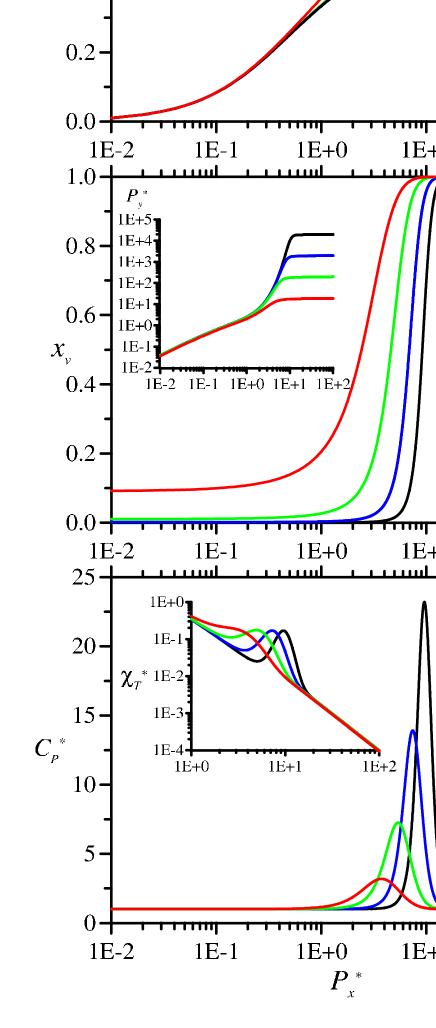
Figure 2: Orientational ordering transition of hard rectangles for pore-width $H^{*}=2$. The length of the rectangle is varied via $L^{*}=2-10^{-\epsilon}$, where $\epsilon=1$, 2, 3 and 4. The packing fraction ($\eta$), the mole fraction of vertically oriented particles ($x_{v}$) and the isobaric heat capacity ($C_{p}$) are shown as a function of horizontal pressure ($P_{x}$) in the upper, middle and lower panels, respectively. The dashed curve in the upper panel is the Tonks-equation of horizontally ordered hard rectangles. The vertical pressure ($P_{y}$) and the isothermal compressibility ($\chi_{T}$) are also shown in the insets of middle and lower panels. All quantities are in dimensionless unit, i.e. $H^{*}=H/D$, $L^{*}=L/D$, $P_{x}^{*}=\beta P_{x}LD$, $P_{y}^{*}=\beta P_{y}LD$, $\chi_{T}^{*}=k_{B}T\chi_{T}/(LD)$ and $C_{P}^{*}=C_{p}/Nk_{B}$.

Fig. 2 presents together the results of Eqs. (22)-(25) for varying $L$ at $H^{*}=2$. One can see that a structural transition occurs between horizontally and vertically ordered fluids. The transition becomes more pronounced as $L^{*}=2-10^{-\epsilon}$ goes to $H^{*}$ with increasing $\epsilon$. To understand this phenomenon, we examine the low, intermediate and high-pressure cases as obtained from the equation of state [Eq. (22)]. At very low pressures the interaction term $(aD+bL)/(a+b)$ in Eq. (22) becomes negligible with respect to $P^{-1}$ and the ideal gas law ($P_{x}^{*}=\eta$) can be reproduced, i.e. all curves go together in the $\eta-P_{x}^{*}$ diagram for $P_{x}^{*}<1$. At intermediate pressures, $b$ becomes much larger than $a$ with increasing $\epsilon$, i.e. $(aD+BL)/(a+b)\approx L$. From this fact we get that

$$\eta=LD\left[H\left(\frac{1}{P}+L\right)\right]^{-1},$$ (26)

which is the well-known Tonks-equation of horizontally ordered rectangles. The close packing density of this fluid can be obtained in the $P\to\infty$ limit, and we get that $\eta_{cp}=D/H$ ($\eta_{cp}=1/2$ in Fig. 2). One can see that the perfect agreement between Eqs. (22) and (26) extends to the direction of higher pressures with increasing $\epsilon$. The reason for this is that the vertical accessible distance and the corresponding fluctuations in $y$ positions shrink with $L\to H$ for particles in vertical direction, while particles can occupy the same vertical interval and $y$ fluctuations are not affected as $L\to H$ for particles with horizontal direction. Practically this manifests in prefactors of $a$ and $b$, where ($H-L$) and ($H-D$) are the accessible distances along the $y$ direction. Therefore $b$ is the dominant factor for $L\to H$. However, this is not the case for very high pressures, because we reach the close packing at $\eta=0.5$ with the horizontally ordered particles, while the vertically ordered fluid has the maximum density at $\eta=L/H$ , which is almost one in our case. Therefore the system of rectangles must undergo a structural transition for $\eta>0.5$. In this case $a$ overcomes $b$ and $(aD+BL)/(a+b)\approx D$, because $\tilde{K}_{v,v}$ becomes much larger than $\tilde{K}_{h,h}$ with $P\to\infty$. In this case the system becomes a fluid of vertically ordered rectangles, which can be described by the following Tonks-equation

$$\eta=LD\left[H\left(\frac{1}{P}+D\right)\right]^{-1},$$ (27)

which gives the close packing density ($\eta=L/H$) in the limit $P\to\infty$. Practically the suppression of horizontal fluctuations is the driving force of the structural transition, which manifests in a crossing between $a$ and $b$ interaction terms. The structural change can be seen very clearly in the mole fraction, too, because $x_{v}\approx 0$ for intermediate pressures ($b>a$), while $x_{v}\approx 1$ for high pressures ($b<a$). The heat capacity is the same in the low and high pressure limit as $C_{P}^{*}(P\to 0)=C_{P}^{*}(P\to\infty)=1$, but it exhibits a peak at the transition region. As the transition becomes sharper ($L\to H$), the peak is narrower and higher. The structural transition has a signature in the compressibility factor, too, since the system can be compressed more in the transition region than in the outer region. It can be seen from Eq. (24) that the system becomes incompressible with increasing pressure as $\chi_{T}^{*}(P\to 0)=0$. The vertical pressure increases with $P$ in the horizontal fluid phase, while it saturates in the vertical fluid one. Its maximum value is given by $P_{y}^{*}(P\to\infty)=L/(H-L)$, which can be obtained from Eq. (23) using $a\gg b$ and $\eta\to L/H$.

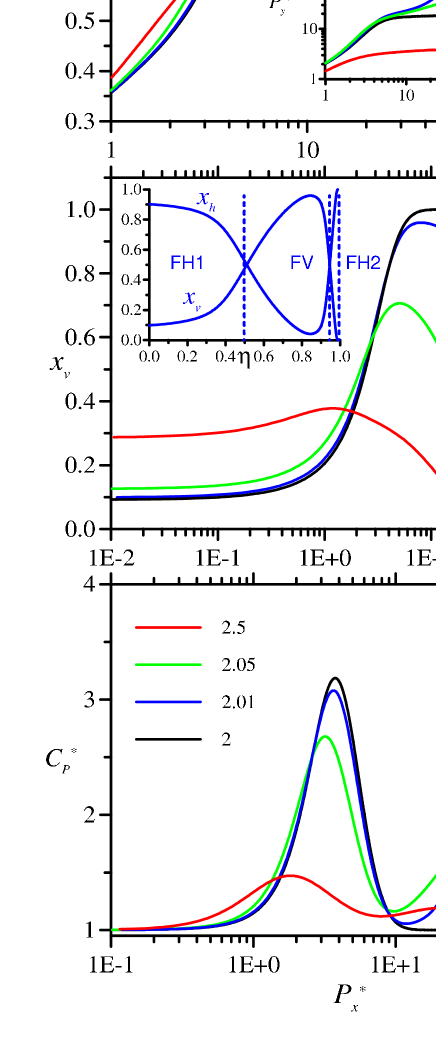
Figure 3: Positional and orientational ordering transitions of hard rectangles at $L^{*}=1.9$. The width of the pore is varied from $H^{*}=2$ to $H^{*}=2.5$. The packing fraction ($\eta$), the mole fraction of vertically oriented particles ($x_{v}$) and the isobaric heat capacity ($C_{p}$) as a function of horizontal pressure are shown in the upper, middle and lower panels, respectively. The mole fractions of vertically ($x_{v}$) and horizontally ($x_{h}$) ordered rectangles as a function of packing fraction is shown in the inset of the middle panel, while the vertical pressure ($P_{y}$) is presented in the inset of upper panel. The vertical dashed lines are the packing fractions of the close packing structures in FH1, FV and FH2 phases, respectively. All quantities are in dimensionless unit.

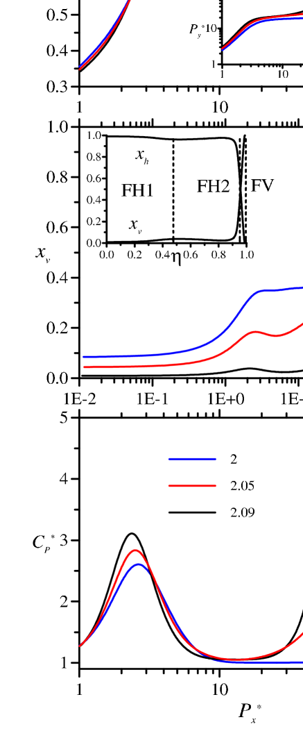
Figure 4: Same as Fig. 3 for pore-width $H^{*}=2.1$. The length of the rectangle is varied from $L^{*}=2$ to $L^{*}=2.09$.

In wider pores ($H^{*}>2$), where the horizontal particles can pass each other, the close packing structure and the corresponding volume fractions depend on the length of the particle. For $L<2D$ the two layer structure (FH2) is the most dense with $\eta_{cp}=2D/H$, while FV has the highest close packing for $L>2D$ with $\eta_{cp}=L/H$. Fig. 3 shows how the FH2 structure conquers the high density region as the pore is widening from $H^{*}=2$ to $H^{*}=2.5$ at $L^{*}=1.9$. One can observe two structural transitions with increasing horizontal pressure: a FH1-FV transition occurs when the packing fraction exceeds the close packing of the FH1 structure ($\eta_{cp}(\rm FH1)=D/H$), while the FV-FH2 transition takes place at the vicinity of $\eta\approx\eta_{cp}(\rm FV)=L/H$. This manifests in two inflection points in the $\eta-P_{x}^{*}$ curve, two plateaus in $P_{y}^{*}$ and two peaks in $C_{P}^{*}$. The stabilization of the FH1 phase at low densities is due to the wall, because the pore is wider for particles having horizontal orientation than for those with vertical orientation, i.e. a larger portion of the pore can be occupied with the FH1 structure. As the close packing of FH1 is approached, the system must change its structure to avoid the forbidden overlapping states. It chooses the FV structure, because it provides plenty of room along the $x$ axis with a price of less room along $y$ axis. This is entropically better than going directly to the FH2 structure, where the room for the particles is less both in $x$ and $y$ directions. However this is not the case in the vicinity of the close packing density of the FV phase, because particles get in contact and are forced to choose the more packed FH2 structure, where the particles still have some room along the $x$ and $y$ axes. The FH1-FV and FV-FH2 transitions are getting sharper as $L\to 2D$ ($L<2D$) and $H\to 2D$ ($H>2D$), while they become smoother with increasing pore width. For example the appearance of mixed phases at low and intermediate densities for $H^{*}=2.5$ is due to the increased room available along the horizontal direction for both vertical and two-layer structures. The FH1-FV-FH2 phase sequence is replaced by FH1-FH2-FV if $L>2D$, which is displayed in Fig 4. At $L=2D$ only a structural transition occurs between FH1 and a mixed phase with more particles in FH2 structure. The emergence of this mixed phase is due to the fact that the close packing densities of FH1 and FV are identical at $L=2D$ ($\eta_{cp}(\rm FV)=\eta_{cp}(\rm FH2)$). This manifest clearly in the one-peak structure of $C_{P}^{*}$, which is located in the vicinity of the close packing density of the FH1 phase. With gradual increment of $L$ to $H$ one can see the emergence of a new inflection point in the $\eta-P_{x}^{*}$ curve, a second plateau in $P_{y}^{*}$ and a second peak in $C_{P}^{*}$ in the vicinity of $\eta\approx\eta_{cp}(\rm FH2)=2D/H$. The transition is getting sharper and the phases become less mixed as $L\to H$, because the vertical fluctuations are suppressed.

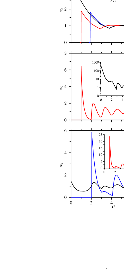
Figure 5: Pair correlation functions of FH1 (upper panel), FV (middle panel) and FH2 (lower panel) structures. Three different functions are shown for a particle fixed at the lower wall: in $g_{hh}^{l}(x)$ [$g_{hh}^{u}(x)$] both particles are horizontal and the second one is at the lower [upper] wall, while in $g_{vv}^{l}(x)$ both particles are vertical and the second one is at the lower wall. These results are obtained with the FMT and the following parameters: $H^{*}=2.05$ , $L^{*}=1.9$ and $\eta=0.2$ (upper panel), $H^{*}=2.05$ , $L^{*}=1.9$ and $\eta=0.68$ (middle panel) and $H^{*}=2.1$, $L^{*}=2.05$ and $\eta=0.8$ (lower panel).

Finally we present our fundamental measure theory (FMT) results for the structural properties of the three different structures observed. Here we do not go into the details of the theory, as it can be found in 39 . All correlation functions are computed for a fixed particle in contact with the lower wall. The following pair correlation functions are determined as a function of horizontal distance $(x)$: in $g_{hh}^{l}(x)$ both particles are in horizontal orientation and are located at the contact with the lower wall, in $g_{hh}^{u}(x)$ both particles are in horizontal orientation and the second particle is at the upper wall, while in $g_{vv}^{l}(x)$ and $g_{vv}^{u}(x)$ both particles are in vertical orientation. The typical correlation functions of the FH1, FH2 and FV structures are shown together in Fig. 5. At $H^{*}=2.05$, $L^{*}=1.9$ and $\eta=0.2$ we find a FH1 structure, as FMT gives $x_{h}=0.84$ ($x_{v}=0.16$). One can see that this is a weakly correlated system as all correlation functions go quickly to 1. The correlation between two horizontal particles is maximum when they are one above the other (see $g_{hh}^{u}(x)$). However this configuration happens rarely because it is more common that the horizontal particles are in the same layer. Note that $g_{vv}^{l}(x)$ and $g_{vv}^{u}(x)$ are the same in this case, and show very small correlations at short distances. At $\eta=0.68$ the stable structure is FV, because $x_{v}=0.84$ and $x_{h}=0.16$. The correlation between vertical particles at both walls is identical. $g_{vv}^{l}(x)$ shows the typical fluid structure of vertically ordered particles as the period of the damped oscillation is close to $D$. The correlations between vertical particles are relatively high when the particles are in contact and decay with distance. The behavior of $g_{hh}^{u}(x)$ gives further information about the microstructure of the FV structure for wider pores ($H>2D$). One can see an extremely strong correlation for very short distances between horizontal particles (see the log scale in the graph). This is due to the fact that the density is very high and almost all particles are vertical. To maintain the high density of the system the horizontal particles must form dimers. For larger distances the correlations decay to 1 with some oscillations. The correlations in the same layer ($g_{hh}^{l}(x)$) have a similar behavior but with a forbidden region and with the first peak much smaller than $g_{hh}^{u}(0)$. These results show very clearly that the FV structure of wide pores consists of long chains of vertical particles which are interrupted mainly by the dimers of horizontal particles. This is not the case in narrow pores ($H<2D$), where dimers cannot form along the $y$ direction. The structure of FH2 is examined at $H^{*}=2.1$, $L^{*}=2.05$ and $\eta=0.8$, where $x_{h}=0.93$ ($x_{v}=0.07$). Here $g_{hh}^{u}(x)$ shows very clearly that the two layers of horizontal particles are quite uncorrelated since $g_{hh}^{u}(x)$ oscillates always very close to 1. However in the same layer $g_{hh}^{l}(x)$ shows that the horizontal particles are more correlated with a period close to $L$. In both $g_{hh}^{l}(x)$ and $g_{hh}^{u}(x)$ there exist two kinds of peaks, the main ones have a period of $\sim 2L$, while the secondary smaller peaks are dephased by $\sim D$ due to the presence of few vertical particles. The correlation between vertical particles ($g_{vv}(x)$) shows a first peak at $x=D$ (particles at contact) which is significantly higher than the rest of the peaks. This means that the vertical particles can be found mainly in the form of dimers in the sea of horizontal particles. As all correlations are short ranged, FH2 is really a fluid phase without signs of solid-like order.

IV Discussion

We have shown that the structure of the rectangles can be manipulated in slit-like pore by an external force acting along the longitudinal direction. Upon increment of the force the particles undergo one or two structural rearrangements. One or two layers can form with horizontally ordered particles, while only one layer can be generated with vertically ordered ones. As the thermodynamic quantities do not exhibit singularities, the possibility of a genuine phase transition can be excluded in our model. This is a consequence of the form of the integral kernel (Eq. 10), which is positive for arbitrary pressure and molecular parameters 40 ; 41 . However, the inflection points of the equation of state, plateaus in vertical pressure and peaks in the heat capacities are hallmarks of the structural phase transitions. As the system can be trapped easily by the suppression of room available for the particles along vertical direction, the system can get into jammed and glass states as happens with hard disks confined into a 2D slit-pore 42 ; 43 ; 44 . In addition to this, the very strong structural transition as occurs in our model in the limit of $L\to H$ can be viewed as a first order transition in simulation studies 45 . The advantage of our TOM formalism is that it provides exact thermodynamic results and some structural information.

It is particularly interesting in this model that anchoring of the particles from planar to hometropic takes place with increasing longitudinal pressure or density and the planar ordering effect of the hard walls does not prevail at high pressures. Recently a density induced planar to homeotropic ordering was observed at hard walls in the system of stiff ring polymers 46 . Therefore it is feasible that strongly confined hard rods can also exhibit planar- homeotropic ordering transition if the length of the rods is close to the pore width. In this regard further studies are needed.

- (1) M. Schmidt and H. Löwen, PRE 55, 7228 (1997).
- (2) A. Fortini and M. Dijkstra, J. Phys.: Condens. Matter 18, L371 (2006).
- (3) R. van Roij, M. Dijkstra, and R. Evans, EPL 49, 350 (2000).
- (4) M. Dijkstra, R. van Roij, and R. Evans, PRE 63, 051703 (2001).
- (5) R. van Roij, M. Dijkstra, and R. Evans, J. Chem. Phys. 113, 7689 (2000).
- (6) M. C. Lagomarsino, M. Dogterom, and M. Dijkstra, J. Chem. Phys. 119, 3535 (2003).
- (7) R. Aliabadi, M. Moradi and S. Varga, PRE 92, 032503 (2015).
- (8) D. de las Heras, E. Velasco, and L. Mederos, PRL 94, 017801 (2005).
- (9) D. de las Heras, E. Velasco, and L. Mederos, PRE 74, 011709 (2006).
- (10) K. W. Wojciechowski and D. Frenkel, Comp. Methods in Science and Tech. 10, 235 (2004).
- (11) A. Donev, J. Burton, F. H. Stillinger and S. Torquato, PRB 73, 054109 (2006).
- (12) C. Avendano and F. A. Escobedo, Soft Matter 8, 4675 (2012).
- (13) H. Schlacken, H.-J. Mogel, and P. Schiller, Mol. Phys. 93, 777 (1998).
- (14) S. Varga and I. Szalai, J. Mol. Liqs. 85, 11 (2000).
- (15) Y. Martínez-Ratón, E. Velasco, and L. Mederos, J. Chem. Phys. 122, 064903 (2005).
- (16) Y. Martínez-Ratón, E. Velasco, and L. Mederos, J. Chem. Phys. 125, 014501 (2006).
- (17) S. Belli, M. Dijkstra and R. van Roij, J. Chem. Phys. 137, 124506 (2012).
- (18) J. Kundu and R. Rajesh, PRE 89, 052124 (2014).
- (19) T. Nath, D. Dhar and R. Rajesh, EPL 114, 10003 (2016).
- (20) J. Galanis, D. Harries, D. L. Sackett, W. Losert and R. Nossal, PRL 96, 028002 (2006).
- (21) R. S. Mclean, X. Huang, C. Khripin, A. Jagota and M. Zheng, Nano Letters 6, 55 (2006).
- (22) K. Zhao, C. Harrison, D. Huse, W. B. Russel and P. M. Chaikin, PRE 76, 040401 (2007).
- (23) K. Zhao, R. Bruinsma, and T. G. Mason, Proc. Natl. Acad. Sci. U.S.A. 108, 2684 (2011).
- (24) R. Sánchez and L. A. Aguirre-Manzo, Phys. Scr. 90, 095002 (2015).
- (25) L. Walsh and N. Menon, J. Stat. Mech.: Theory and Experiment 2016, 083302 (2016).
- (26) W.-Y. Zhang, Y. Jiang, and J. Z. Y. Chen, PRL 108, 057801 (2012).
- (27) J. Z. Y. Chen, Soft Matter 9, 10921 (2013).
- (28) M. González-Pinto, Y. Martínez-Ratón, and E. Velasco, PRE 88, 032506 (2013).
- (29) M. E. Ferraro, T. M. Truskett and R. T. Bonnecaze, PRE 93, 032606 (2016).
- (30) Y. Li, H. Miao, H. Ma, and J. Z. Y. Chen, Soft Matter 9, 11461 (2013).
- (31) D. de las Heras and E. Velasco, Soft Matter 10, 1758 (2014).
- (32) T. Geigenfeind, S. Rosenzweig, M. Schmidt, and D. de las Heras, J. Chem. Phys. 142, 174701 (2015).
- (33) Y. Martínez-Ratón, PRE 75, 051708 (2007).
- (34) D. A. Triplett and K. A. Fichthorn, PRE 77, 011707 (2008).
- (35) J. L. Lebowitz, J. K. Percus, and J. Talbot, J. Stat. Phys. 49, 1221 (1987).
- (36) D. A. Kofke and A. J. Post, J. Chem. Phys. 98, 4853 (1993).
- (37) Y. Kantor and M. Kardar, EPL 87, 60002 (2009).
- (38) P. Gurin and S. Varga, J. Chem. Phys. 142, 224503 (2015).
- (39) M. González-Pinto, Y. Martínez-Ratón, S. Varga, P. Gurin and E. Velasco, J. Phys.: Condens. Matter 28, 244002 (2016).
- (40) L. van Hove, Physica 16, 137 (1950).
- (41) J. A. Cuesta and A. Sánchez, J. Stat. Phys. 115, 869 (2004).
- (42) S. S. Ashwin and R. K. Bowles, PRL 102, 235701 (2009).
- (43) M. J. Godfrey and M. A. Moore, PRE 89, 032111 (2014).
- (44) M. J. Godfrey and M. A. Moore, PRE 91,022120 (2015).
- (45) P. Gurin, S. Varga and G. Odriozola, PRE 94, 050603(R) (2016).
- (46) P. Poier, S. A. Egorov, C. N. Likos and R. Blaak, Soft Matter 12, 7983 (2016).