Massive MIMO Pilot Decontamination and Channel Interpolation via Wideband Sparse Channel Estimation

Abstract

We consider a massive MIMO system based on Time Division Duplexing (TDD) and channel reciprocity, where the base stations (BSs) learn the channel vectors of their users via the pilots transmitted by the users in the uplink (UL). It is well-known that, in the limit of very large number of BS antennas, the system performance is limited by pilot contamination, due to the fact that the same set of orthogonal pilots is reused in multiple cells. In the regime of moderately large number of antennas, another source of degradation is channel interpolation because the pilot signal of each user probes only a limited number of OFDM subcarriers and the channel must be interpolated over the other subcarriers where no pilot symbol is transmitted. In this paper, we propose a low-complexity algorithm that uses the received UL wideband pilot snapshots in an observation window comprising several coherence blocks (CBs) to obtain an estimate of the angle-delay Power Spread Function (PSF) of the received signal. This is generally given by the sum of the angle-delay PSF of the desired user and the angle-delay PSFs of the copilot users (CPUs), i.e., the users re-using the same pilot dimensions in other cells/sectors. We propose supervised and unsupervised clustering algorithms to decompose the estimated PSF and isolate the part corresponding to the desired user only. We use this decomposition to obtain an estimate of the covariance matrix of the user wideband channel vector, which we exploit to decontaminate the desired user channel estimate by applying Minimum Mean Squared Error (MMSE) smoothing filter, i.e., the optimal channel interpolator in the MMSE sense. We also propose an effective low-complexity approximation/implementation of this smoothing filter. We use numerical simulations to assess the performance of our proposed method, and compare it with other recently proposed schemes that use the same idea of separability of users in the angle-delay domain.

I Introduction

Consider a massive MIMO multi-cell system with $M$ antenna per each base station (BS), per-cell processing, Orthogonal Frequency Division Multiplexing (OFDM), Time Division Duplexing (TDD), and reciprocity-based channel estimation as in [1, 2, 3]. In such systems, time is divided into several slots, where in each slot users are scheduled to send uplink (UL) pilot signals in order to allow the BS to estimate their channel vectors. The BS exploits the UL-DL reciprocity and uses the resulting channel estimates to coherently detect data from the users in the UL and precode data to the users in the DL. A family of mutually orthogonal pilot sequences are obtained in the time-frequency domain by assigning to each pilot a different set of signal dimensions in the tessellation of the time-frequency plane under the OFDM [1] or, more in general, by sharing all the signal dimensions but assigning to the pilots mutually orthogonal symbol sequences across all signal dimensions (e.g., see [4]). Due to limited channel coherence time, the signal dimensions in each UL-DL scheduling slot are limited. Consequently, also the number of UL pilot signal dimensions is limited, resulting in a limited number of orthogonal pilots. Therefore, to simultaneously serve several users across the whole system, pilots must be reused in multiple cells according to a specific reuse pattern [1]. As a result, the channel estimation during the UL pilot transmission is severely degraded by the interference received from the users in neighboring cells (or sectors) re-using the same pilot sequences as the users inside the cell; these users are referred to as copilot users (CPUs). Such a phenomenon is called pilot contamination. It is well-known that pilot contamination becomes the only limiting factor on the spectral efficiency of the system in the asymptotic limit where the number of BS antennas $M\rightarrow\infty$ but the number of users per cell $K$ is kept finite [1, 5]. In the more realistic case of large but finite $M$ and $K$ with $M\gg K$, the pilot contamination still represents an important source of degradation especially for the edge users lying on the cell boundary [6, 7, 8].

I-A Approaches to pilot decontamination

Several approaches have been proposed to cope with pilot contamination. In [9], it is observed that if multipath components (MPCs) of the channel vectors of the users have a limited angular spread (spatial correlation), it is possible to coordinate the pilot transmission in adjacent cells such that the channels of CPUs are confined in nearly orthogonal subspaces due to their angular diversity. However, in order to effectively separate CPUs, the covariance information (or subspace information), i.e., the second-order statistics of users’ channel vectors, must be known at the BS. A similar a priori statistical knowledge is used in [10, 11] in the so-called JSDM scheme to reuse pilots in the same cell in order to decrease the pilot dimension overhead. More generally, it has been shown in [12] that if the covariance matrices of the users and their CPUs are available at the BS and satisfy certain mild conditions of linear independence, pilot contamination in the limit of $M\rightarrow\infty$ can be completely eliminated. However, this requires the knowledge of the user channel covariance matrices, which is itself difficult to obtain precisely due to pilot contamination.

A quite different approach is proposed in [13], in which no a priori knowledge of subspace is needed. Instead, it is noticed that when the number of BS antennas $M$ is much larger than the number of per-cell served users $K$, and the power imbalance between the desired and the interfering users is above a certain threshold, the eigenvalues of the sample covariance matrix of the received signal corresponding to the desired users and that corresponding to CPUs in adjacent cells concentrate on “clusters” with disjoint supports. Thus, by distinguishing those clusters, it is possible to identify blindly the desired and the interfering signal subspaces. In contrast to [9, 10, 11], which work only in the presence of spatially correlated channels, the method of [13] would work also with i.i.d. (isotropically distributed) channel vectors, provided that the power imbalance between the desired and the interfering users is sufficiently large and the matrix dimension is large enough such that the eigenvalue clustering is sufficiently sharp. A combination of techniques in [9] and [13], via exploiting both the spatial correlation and power discrimination, has been used in [14].

Another method to cope with pilot contamination consists in “pilot contamination precoding” as proposed in [15]. The main idea is that, due to very large number of BS antennas, the only residual interference that matters after beamforming is the coherent interference due to pilot contamination, which can be eliminated by jointly precoding across neighboring cells (e.g., in the DL using linear precoding or non-linear dirty-paper coding and in the UL using linear interference mitigation or non-linear successive interference cancellation). Such a scheme, however, requires centralized processing of multiple cell sites in order to jointly decode/precode the UL/DL signals; this goes against the beauty and simplicity of massive MIMO, for which single-cell processing is one of the main motivations [1].

In the recent work [16], developed independently and in parallel with our present work, a method for pilot decontamination is proposed by exploiting the fact that the channel vectors of CPUs at a given BS have typically different MPCs in the angle-delay domain. Therefore, if it is possible to identify the MPCs pertaining only to the desired user, the interference due to CPUs can be mitigated by linear space-frequency filtering, thus, mitigating the effect of pilot contamination. Our work is also based on the same idea but differs from [16] in many aspects and generally can achieve much better performance without incurring any additional pilot overhead with respect to the standard pilot schemes used in current systems (e.g., in LTE-TDD [17]). We defer a through comparison of [16] with our work to Section VII-H.

I-B Contribution

In this paper, we pursue a new method for pilot decontamination that has the following advantages:

• Unlike [9, 14, 12], we do not assume a priori knowledge of the channel covariance matrices or centralized coordination of pilot allocation.

• Unlike [13, 14], we do not rely on asymptotic results in random matrix theory, which requires a) i.i.d. isotropic channel vectors (spatially correlated channel vectors along with covariance information in [14]), and b) sufficiently large power imbalance between the users inside and outside the cell.

• Unlike [15], we do not rely on joint precoding and centralized processing. Instead, we apply a strictly uncoordinated per-BS processing.

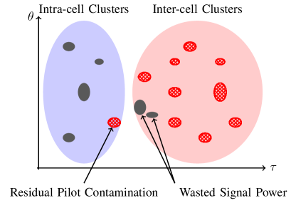
Figure 1: Illustration of the proposed pilot decontamination scheme via exploiting the sparsity of the angle-delay scattering map of the received signal at the BS. The multipath components (MPCs) of the intended user and those of its CPUs are illustrated with grey solid and red dashed bubbles respectively. In this example, most of the MPCs of the user have shorter delays, thus, they can be identified and fairly separated from those of the CPUs via clustering in the delay domain as illustrated in the figure. The red dashed bubbles inside the signal cluster illustrate the residual copilot interference whereas the grey solid bubbles inside the interference cluster correspond to the useful signal wasted because of the delay-based clustering.

Here, we only provide an intuitive explanation of our proposed scheme and postpone the thorough description to Section V. The idea is qualitatively illustrated in Fig. 1. In a massive MIMO macrocell system, the propagation between users and BS antennas occurs through relatively sparse MPCs in the angle-delay domain. We exploit this underlying sparsity to estimate the angle-delay Power Spread Function (PSF) of each user by sampling only a small number of antennas and sending UL pilots only over a small subset of subcarriers. Then, we apply suitable algorithms to cluster the estimated PSF in the angle-delay plane to approximately separate the MPCs belonging to the desired user from those of its CPUs. This is illustrated qualitatively in Fig. 1 for a configuration where clustering is based on the difference of propagation delays, and where the interference due to CPUs can be fairly eliminated by filtering in the delay domain, at the cost of possibly filtering out also some components of the useful signal. Furthermore, once we identified the angle-delay domain clusters pertaining to the desired user’s PSF, we exploit them to obtain a very compact representation of the user wideband covariance matrix over the whole set of OFDM subcarriers. In turns, we use this information for MMSE channel estimation, obtaining at once both decontamination (i.e., the contribution of the CPUs is filtered out by the channel estimator) and channel interpolation over the whole signal bandwidth. We develop a novel computationally efficient channel interpolation method that approximates the Minimum Mean Squared Error (MMSE) smoothing filter. This provides a close-to-optimal MSE channel estimator under the Gaussian statistics and avoids performance degradation incurred due to imperfect instantaneous channel estimation, especially for a moderate number of antennas $M$ [18].

I-C Notation

We represent scalar constants by non-boldface letters (e.g., $x$ or $X$), sets by calligraphic letters (e.g., ${\cal X}$), vectors by boldface small letters (e.g., ${\bf x}$), and matrices by boldface capital letters (e.g., ${\bf X}$). We denote the $i$-th row and the $j$-th column of a matrix ${\bf X}$ with the row-vector ${\bf X}_{i,.}$ and the column-vector ${\bf X}_{.,j}$ respectively. For a $p\times q$ matrix ${\bf X}$, we represent by ${\rm vec}({\bf X})$ the $pq\times 1$ column-vector obtained by stacking the column of ${\bf X}$ on top of each other, where we denote the resulting vector with a blackboard letter ${\mathbb{x}}$ and a matrix consisting of $r$ such vectors by ${\mathbb{X}}=[{\mathbb{x}}_{1},\dots,{\mathbb{x}}_{r}]$. We indicate the Hermitian conjugate and the transpose of a matrix ${\bf X}$ by ${\bf X}^{{\sf H}}$ and ${\bf X}^{\sf T}$ with the same notation being used for vectors and scalars. ${\bf X}\otimes{\bf Y}$ indicates the Kronecker product of the matrices ${\bf X}$ and ${\bf Y}$. We denote the complex and the real inner product between two matrices (and similarly two vectors) ${\bf X}$ and ${\bf Y}$ by ${\langle{\bf X},{\bf Y}\rangle}={\hbox{tr}}({\bf X}^{{\sf H}}{\bf Y})$ and ${\langle{\bf X},{\bf Y}\rangle}_{\mathbb{R}}={\rm Re}[{\langle{\bf X},{\bf Y}\rangle}]$ respectively. We use $\|{\bf X}\|={\langle{\bf X},{\bf X}\rangle}$ for the Frobenius norm of a matrix ${\bf X}$ and $\|{\bf x}\|$ for the $l_{2}$-norm of a vector ${\bf x}$. An identity matrix of order $p$ is represented by ${\bf I}_{p}$. For an integer $k>0$, we use the shorthand notation $[k]$ for $\{1,2,\dots,k\}$.

II Problem Statement

II-A Basic Setup

Our model and system assumptions are standard in most classical works on massive MIMO (e.g., [1, 2, 3, 4, 6, 7, 8, 10, 11, 12, 9, 16]) and recalled here for the sake of completeness and for establishing the notation to be used later. We consider a system with a signal bandwidth of $W$ Hz and a scheduling slot of duration $T_{s}$ sec (including UL pilots, UL payload, and DL payload [1]). The underlying channel fading process has a coherence bandwidth $\Delta f_{c}<W$ and a coherence time $\Delta t_{c}\geq T_{s}$ [19], such that in each scheduling slot we have $\lceil\frac{W}{\Delta f_{c}}\rceil$ frequency sub-bands over which the channel can be considered (approximately) frequency-flat and constant in time over the whole duration of a slot. We call a frequency-time rectangle of bandwidth $\Delta f_{c}$ and duration $T_{s}$ a coherence block (CB). This is illustrated in Fig. 2, where it is seen that the channel is approximately constant over a CB but changes smoothly across different CBs. We denote by $\Delta\tau_{\max}$ the maximum channel delay spread that the system can handle without suffering from inter-block interference between the OFDM symbols [20]. We assume that a set of $B$ OFDM symbols are transmitted inside a time slot, each having a total duration of $T_{\text{OFDM}}=\frac{T_{s}}{B}$ and an effective duration of $T_{u}=T_{\text{OFDM}}-\Delta\tau_{\max}$ after removing the cyclic prefix (CP) of duration $\Delta\tau_{\max}$. The frequency spacing between the subcarriers is given by $\Delta f=\frac{1}{T_{u}}$, thus, each OFDM symbol has $N=\frac{W}{\Delta f}=WT_{u}$ subcarriers. Over each slot, we have a set of $Q=NB=WT_{u}B=WT_{s}(1-\frac{\Delta\tau_{\max}}{T_{\text{OFDM}}})$ signal dimensions.

Figure 2: A slot of duration $T_{s}$ consisting of several OFDM symbols. In this example, a coherence sub-block inside an OFDM symbol contains $D^{\text{c}}_{\text{OFDM}}=4$ signal dimensions (subcarriers), and two OFDM symbols are devoted to pilot transmission, thus, $D^{\text{c}}_{\text{p}}=2D^{\text{c}}_{\text{OFDM}}=8$. We also illustrate a 0-1 pilot sequence that lies on the second training OFDM symbol and probes subcarrier #3 inside each coherence sub-block.

Also, each CB is decomposed into $B$ disjoint sub-blocks lying inside separate OFDM symbols, where each sub-block consists of $D^{\text{c}}_{\text{OFDM}}=\Delta f_{c}T_{u}$ subcarriers and, in total, there are $D^{\text{c}}=BD^{\text{c}}_{\text{OFDM}}$ signal dimensions in each CB. During each slot, some $D^{\text{c}}_{p}$ out of $D^{\text{c}}$ signal dimensions inside each CP are devoted to pilot transmission, while the remaining $D^{\text{c}}_{d}=D^{\text{c}}-D^{\text{c}}_{p}$ signal dimensions are used for UL-DL data transmission. A set of $D^{\text{c}}_{p}$ orthogonal pilot sequences are assigned to $D^{\text{c}}_{p}$ pilot signal dimensions in each CB. The resulting orthogonal pilots are allocated to the users in each cell/sector according to a given reuse pattern (e.g., see [1, 6]), where in reuse patterns with a reuse factor $r\geq 1$, at most $K=\frac{D^{\text{c}}_{p}}{r}$ users can be simultaneously served per cell/sector with mutually orthogonal pilot sequences. In this paper, without any loss of generality, we consider 0-1 pilot sequences (see Fig. 2), where the pilot sequence of each user is transmitted over a single OFDM symbol and places a single “1” in each CB. In this way, each pilot sequence probes one subcarrier per CB (see, e.g., [4]), for a total of $n=\frac{N}{D^{\text{c}}_{\text{OFDM}}}$ subcarriers.

II-B Pilot Contamination

We consider a reference BS called BS₀ and denote by UE_0,k a generic user $k\in[K]$ served by BS₀. As before, we assume that the pilot signal of UE_0,k is transmitted over an individual OFDM symbol and probes a subset of subcarriers $\Omega_{k}\subset[N]$ of size $|\Omega_{k}|=n$. We denote by ${\cal K}_{k}$ the set of all CPUs of UE_0,k, i.e., the users across the whole system that transmit their pilot signal over the same pilot OFDM symbol and over the same set of subcarriers $\Omega_{k}$ as UE_0,k. The received signal of UE_0,k at BS₀ during the pilot transmission is given by

$${\bf y}_{k,s}[\omega]={\bf h}_{k,s}[\omega]+\sum_{k^{\prime}\in{\cal K}_{k}}{\bf h}_{k^{\prime},s}[\omega]+{\bf z}_{s}[\omega],\omega\in\Omega_{k},$$ (1)

where ${\bf h}_{k,s}[\omega]$ and ${\bf h}_{k^{\prime},s}[\omega]$ denote the $M$-dim channel vectors of UE_0,k and its CPUs ${\cal K}_{k}$ to the $M$ antennas at BS₀ at time slot $s$ and subcarrier $\omega$, where ${\bf z}_{s}[\omega]\sim{{\cal C}{\cal N}}(0,\sigma^{2}{\bf I}_{M})$ is the additive white Gaussian noise (AWGN) at subcarrier $\omega$, and where we assumed, without loss of generality, that the transmitted pilot symbols at all subcarriers $\omega\in\Omega_{k}$ are normalized to $1$. From (1), it is seen that during the UL pilot transmission phase, the BS receives the superposition of the channel vector of UE_0,k and that of its CPUs, thus, pilot contamination.

II-C Wideband Pilot Decontamination

We denote by ${\bf H}_{k,s}=\big{[}{\bf h}_{k,s}[1],\dots,{\bf h}_{k,s}[N]\big{]}$ and ${\bf H}_{k^{\prime},s}=\big{[}{\bf h}_{k^{\prime},s}[1],\dots,{\bf h}_{k^{\prime},s}[N]\big{]}$, $k^{\prime}\in{\cal K}_{k}$, the $M\times N$ wideband channel matrices of UE_0,k and its CPUs across $N$ OFDM subcarriers at time slot $s$. We denote by ${\bf S}^{\mathtt{f}}_{k,s}$ an $n\times N$ matrix that has a single $1$ in each row at columns corresponding to the probed subcarriers $\Omega_{k}$ and is $0$ elsewhere. We also assume, for the sake of generality, that during the UL training phase, a subset of size $m$ of the $M$ BS antennas is sampled via an $m\times M$ matrix ${\bf S}^{\mathtt{a}}_{s}$. Thus, from (1), the UL pilot observation for UE_0,k at BS₀ at time slot $s$ can be arranged as a $m\times n$ matrix

$${\bf X}_{k,s}:={\bf S}^{{\mathtt{a}}}_{s}{\bf Y}_{s}{{\bf S}^{{\mathtt{f}}}_{k,s}}^{{{\sf H}}}=\widetilde{{\bf H}}_{k,s}+\sum_{k^{\prime}\in{\cal K}_{k}}\widetilde{{\bf H}}_{k^{\prime},s}+\widetilde{{\bf Z}}_{k,s},$$ (2)

where ${\bf Y}_{s}=\big{[}{\bf y}_{s}[1],\dots,{\bf y}_{s}[N]\big{]}$ denotes the $M\times N$ wideband signal received across all the subcarriers, and where $\widetilde{{\bf H}}_{k,s}={\bf S}^{{\mathtt{a}}}_{s}{\bf H}_{k,s}{{\bf S}^{{\mathtt{f}}}_{k,s}}^{{{\sf H}}}$ contains the channel coefficients of UE_0,k corresponding to the $m$ sampled antennas and the $n$ probed subcarriers, with the same interpretation holding for $\widetilde{{\bf H}}_{k^{\prime},s}$, $k^{\prime}\in{\cal K}_{k}$, and $\widetilde{{\bf Z}}_{k,s}$. We denote by ${\mathbb{h}}_{k,s}={\rm vec}({\bf H}_{k,s})$ and ${\mathbb{h}}_{k^{\prime},s}={\rm vec}({\bf H}_{k^{\prime},s})$, $k^{\prime}\in{\cal K}_{k}$, the wideband channel vectors obtained after vectorization. Applying the ${\rm vec}$ operator and using the identity ${\rm vec}({\bf A}{\bf B}{\bf C})=({\bf C}^{\sf T}\otimes{\bf A}){\rm vec}({\bf B})$, we can write (2) as

$${\mathbb{x}}_{k,s}={\mathbb{S}}_{k,s}{\mathbb{y}}_{k,s}=\widetilde{{\mathbb{h}}}_{k,s}+\sum_{k^{\prime}\in{\cal K}_{k}}\widetilde{{\mathbb{h}}}_{k^{\prime},s}+\widetilde{{\mathbb{z}}}_{k,s},$$ (3)

where ${\mathbb{S}}_{k,s}={\bf S}^{\mathtt{f}}_{k,s}\otimes{\bf S}^{\mathtt{a}}_{s}$ and where $\widetilde{{\mathbb{h}}}_{k,s}={\mathbb{S}}_{k,s}{\mathbb{h}}_{k,s}$, $\widetilde{{\mathbb{h}}}_{k^{\prime},s}={\mathbb{S}}_{k^{\prime},s}{\mathbb{h}}_{k^{\prime},s}$, $k^{\prime}\in{\cal K}_{k}$. With this notation, the objective of pilot decontamination can be stated as follows.

Pilot Decontamination: Given the noisy and contaminated UL wideband pilot sketches $\{{\mathbb{x}}_{k,s}:s\in[{\sf w}]\}$ of the desired user UE_0,k across ${\sf w}$ time slots, construct an estimator for its wideband channel vector ${\mathbb{h}}_{k,s}$ (equivalently, its wideband channel matrix ${\bf H}_{k,s}$) at the next time slots $s\geq{\sf w}+1$.      $\lozenge$

To explain this better, let us define the wideband (space-frequency) covariance matrices of UE_0,k and of its CPUs by ${\bf C}_{k}={\mathbb{E}}[{\mathbb{h}}_{k,s}{\mathbb{h}}_{k,s}^{{\sf H}}]$ and ${\bf C}_{k^{\prime}}={\mathbb{E}}[{\mathbb{h}}_{k^{\prime},s}{\mathbb{h}}_{k^{\prime},s}^{{\sf H}}]$, $k^{\prime}\in{\cal K}_{k}$, independent of $s$ by the WSS assumption (see Section III-A). Note that if these covariance matrices are available at BS₀, using the fact that the channel vectors ${\mathbb{h}}_{k,s}$ and $\{{\mathbb{h}}_{k^{\prime},s}:k^{\prime}\in{\cal K}_{k}\}$ are independent vector-valued stationary Gaussian random processes (see Section III-A for more details), the immediate answer to our estimation problem for pilot decontamination would be the MMSE smoothing filter, given by

$$\widehat{{\mathbb{h}}}_{k,s}=\hbox{\boldmath$\Sigma$}_{{\mathbb{h}}_{k},{\mathbb{x}}_{k}}{\bf C}_{{\mathbb{x}}_{k}}^{-1}{\mathbb{x}}_{k,s}={\bf C}_{k}{\mathbb{S}}^{{\sf H}}_{k,s}\left(\sigma^{2}{\bf I}_{mn}+{\mathbb{S}}_{k,s}\left({\bf C}_{k}+\sum_{k^{\prime}\in{\cal K}_{k}}{\bf C}_{k^{\prime}}\right){\mathbb{S}}^{{\sf H}}_{k,s}\right)^{-1}{\mathbb{x}}_{k,s},$$ (4)

where $\hbox{\boldmath$\Sigma$}_{{\mathbb{h}}_{k},{\mathbb{x}}_{k}}:={\mathbb{E}}[{\mathbb{h}}_{k,s}{\mathbb{x}}_{k,s}^{{\sf H}}]={\bf C}_{k}{\mathbb{S}}^{{\sf H}}_{k,s}$, and where we used ${\mathbb{S}}_{k,s}^{{\sf H}}{\mathbb{S}}_{k,s}={\bf I}_{mn}$. In practice, however, ${\bf C}_{k}$ and ${\bf C}_{k^{\prime}}$, $k^{\prime}\in{\cal K}_{k}$, are not available and should be estimated from the noisy and contaminated pilot sketches $\{{\mathbb{x}}_{k,s}:s\in[{\sf w}]\}$. With this brief explanation, the problems we are addressing in this paper are as follows:

1. How can we efficiently estimate the wideband covariance matrices of the desired user and of the CPUs from the subsampled and contaminated observations $\{{\mathbb{x}}_{k,s}:s\in[{\sf w}]\}$? We address this question by estimating the contaminated wideband channel covariance matrix ${\bf C}_{k}+\sum_{k^{\prime}\in{\cal K}_{k}}{\bf C}_{k^{\prime}}$ via exploiting the sparsity of MPCs in the angle-delay domain (Section IV), and applying suitable clustering techniques in the angle-delay domain to decompose approximately the resulting contaminated wideband covariance matrix into its signal and interference parts ${\bf C}_{k}$ and $\sum_{k^{\prime}\in{\cal K}_{k}}{\bf C}_{k^{\prime}}$ (Section V-B and V-C).

2. How can we approximate the MMSE smoothing filter (4) in an efficient way, not requiring inversion of a $mn\times mn$ matrix and complicated and time-consuming matrix-matrix multiplication in (4)? We address this complexity issue by developing computationally-efficient pilot decontamination and channel interpolation algorithms (Section VI and Appendix A).

III Wideband Channel Model

III-A WSS-US Assumption

The COST 2100 channel model consists (up to some drastic simplifications) of clusters of MPCs and visibility regions [21]. The propagation between a BS and a user inside the intersection of multiple visibility regions occurs through all corresponding clusters (see Fig. 3).

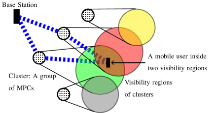
Figure 3: A sketch of the cluster and visibility regions of the COST2100 model.

This implies that the statistics of the channel between a BS and a user remains constant in time and frequency as long as the user remains in the intersection of same visibility regions. As the user crosses the boundary of some region and enters a new region, the channel statistics typically undergoes a sharp transition. Since moving across the regions occurs at a time scale much larger than moving across one wavelength, it is safe to assume that the channel statistics is piecewise time-invariant with relatively sharp transitions at very low rate compared with the signaling rate. In this paper, for simplicity, we neglect such transitions and suppose a time-invariant second-order statistics for the channel during the whole communication interval, i.e., the channel process is assumed to remain (locally) Wide Sense Stationary (WSS) over time. Furthermore, the MPCs originated by different users and/or different scattering clusters are assumed to be mutually uncorrelated (US assumption). Finally, since each MPC is formed by a very large number of elementary multipath contributions, superimposing with different phases, invoking the Central Limit Theorem it is widely accepted to model the MPC coefficients as complex circularly symmetric Gaussian [19, 20].

III-B Sparsity in the Angle-Delay Domain

Without loss of generality, we focus on a single BS-user pair and neglect the user and BS indices to simplify the notation. Also, for simplicity, we adopt a discrete multipath model [22, 23, 24, 25, 4] with $L$ MPCs, each of which is characterized by an Angle of Arrival (AoA) $\theta_{l}$ and a delay $\tau_{l}$. All the results of this paper extend to the general case of mixed-type discrete-continuous scattering as long as the MPCs have a limited angle-delay support. In each time slot $s$, the UL channel is given by the vector impulse response

$$\check{{\bf h}}_{s}(\tau)=\sum_{l=1}^{L}\rho_{s,l}{\bf a}(\theta_{l})\delta(\tau-\tau_{l}),$$ (5)

where ${\bf a}(\theta)$ denotes the array response at AoA $\theta\in[-\theta_{\max},\theta_{\max}]$, whose $k$-th component is $[{\bf a}(\theta)]_{k}=e^{jk\frac{2\pi d}{\lambda}\sin(\theta)}$, where $\lambda=\frac{c_{0}}{f_{0}}$ denotes the wavelength ($c_{0}$ denoting the speed of light) and where $f_{0}$ is the carrier frequency. We assume that the array elements have the uniform spacing $d=\frac{\lambda}{2\sin(\theta_{\max})}$, thus, $[{\bf a}(\theta)]_{k}=e^{jk\pi\frac{\sin(\theta)}{\sin(\theta_{\max})}}$. As said before, from the WSS-US and Gaussian assumption, we have that the discrete-time path gain processes $\{\rho_{s,l}:s\in{\mathbb{Z}}\}$ are stationary with respect to the (slot) time index $s$ and independent across $l$. Furthermore, we assume no line of sight propagation, yielding $\rho_{s,l}\sim{{\cal C}{\cal N}}(0,\sigma_{l}^{2})$, where $\sigma_{l}^{2}$ denotes the strength of the $l$-th MPC (independent of $s$ because of the WSS assumption).

In the OFDM discrete frequency domain, channel (vector) frequency response corresponding to the impulse response (5) is given by

$${\bf h}_{s}[\omega]=\sum_{l=1}^{L}\rho_{s,l}{\bf a}(\theta_{l})e^{-j\frac{2\pi}{N}W\tau_{l}(\omega-1)},\ \omega\in[N],$$ (6)

such that, as anticipated in Section II, the wideband channel matrix at slot $s$ is given by

$${\bf H}_{s}=\Big{[}{\bf h}_{s}[1],{\bf h}_{s}[2],\dots,{\bf h}_{s}[N]\Big{]}.$$ (7)

We define the $N$-dim vector ${\bf b}(\tau)$, whose $\omega$-th component given by $[{\bf b}(\tau)]_{\omega}=e^{j\frac{2\pi}{N}W\tau(\omega-1)}$. Thus, we can write (7) more compactly as

$${\bf H}_{s}=\sum_{l=1}^{L}\rho_{s,l}{\bf a}(\theta_{l}){\bf b}(\tau_{l})^{{\sf H}}.$$ (8)

The rows of ${\bf H}_{s}$ correspond to the antenna elements, whereas its columns correspond to the OFDM subcarriers. The vectorized channel vector ${\mathbb{h}}_{s}={\rm vec}({\bf H}_{s})$ is, therefore, given by

$${\mathbb{h}}_{s}=\sum_{l=1}^{L}\rho_{s,l}{\mathbb{a}}(\theta_{l},\tau_{l}),$$ (9)

where ${\mathbb{a}}(\theta,\tau)={\rm vec}({\bf a}(\theta){\bf b}(\tau)^{{\sf H}})\in{\mathbb{C}}^{MN}$ denotes the array response in the angle-delay $(\theta,\tau)$. Since the MPC coefficients $\rho_{s,l}\sim{{\cal C}{\cal N}}(0,\sigma_{l}^{2})$ are independent and circularly symmetric Gaussian variables, from (6) it is immediate to check that the statistics of ${\bf h}_{s}[\omega]$ are invariant under circular shifts (with period $N$) in $\omega$, implying stationarity in the frequency domain.

III-C Antenna-Frequency Sampling

As explained in Section II, without any loss of generality, we can assume that a UL pilot sequence for each user probes its channel over a subset of subcarriers in an individual OFDM symbol. Also, the pilot corresponding to different users are sent either across different OFDM symbols (disjoint in time) or across the same OFDM symbol but on disjoint set of subcarriers (disjoint in frequency). As before, we focus on a single user and denote by ${\cal I}^{\mathtt{f}}_{s}=\{c^{\mathtt{f}}_{s,1},\dots,c^{\mathtt{f}}_{s,n}\}$ the indices of the subcarriers acquired for this user at slot $s$. In addition, we consider the general case where also the antennas may be subsampled. This is done for the sake of generality, and also because one may wish to exploit the channel spatial correlation and reduce the sampling overhead at the receiver side. We denote by ${\cal I}^{\mathtt{a}}_{s}=\{c^{\mathtt{a}}_{s,1},\dots,c^{\mathtt{a}}_{s,m}\}$ the indices of the antennas sampled at time slot $s$. We define $n\times N$ and $m\times M$ selection (or sampling) matrices ${{\bf S}_{s}^{\mathtt{a}}}$ and ${{\bf S}_{s}^{\mathtt{f}}}$, where $[{{\bf S}_{s}^{\mathtt{a}}}]_{i,c^{\mathtt{a}}_{s,i}}=1$ and $[{{\bf S}_{s}^{\mathtt{f}}}]_{j,c^{\mathtt{f}}_{s,j}}=1$, for $i\in[n]$ and $j\in[m]$. The sampled channel matrix at slot $s$ is given by $\widetilde{{\bf H}}_{s}={{\bf S}_{s}^{\mathtt{a}}}{\bf H}_{s}{{{\bf S}_{s}^{\mathtt{f}}}}^{{\sf H}}$. Using the ${\rm vec}$ notation, this can be written as

$$\widetilde{{\mathbb{h}}}_{s} ={\mathbb{S}}_{s}{\mathbb{h}}_{s},$$ (10)

where ${\mathbb{S}}_{s}={{\bf S}_{s}^{\mathtt{f}}}\otimes{{\bf S}_{s}^{\mathtt{a}}}$ is of dimension $mn\times MN$, and where we used the well-known identity ${\rm vec}({\bf A}{\bf B}{\bf C})=({\bf C}^{\sf T}\otimes{\bf A}){\rm vec}({\bf B})$. Notice that ${\mathbb{S}}_{s}{\mathbb{S}}_{s}^{{\sf H}}={\bf I}_{mn}$, and that ${\mathbb{S}}_{s}$ has only a single element equal to $1$ in each row at column indices given by

$${\cal I}_{s}:=\{M(c_{s}^{\mathtt{f}}-1)+c_{s}^{\mathtt{a}}:\ \ c_{s}^{\mathtt{f}}\in{\cal I}_{s}^{\mathtt{f}},\ c_{s}^{\mathtt{a}}\in{\cal I}_{s}^{\mathtt{a}}\}\subseteq[MN].$$ (11)

Using the above notation, the observation at the reference BS corresponding to a generic user (see (2) and (3)) can be written as ${\mathbb{x}}_{s}={\mathbb{S}}_{s}{\mathbb{y}}_{s}$, where

$${\mathbb{y}}_{s}={\mathbb{h}}_{s}+\sum_{j\in{\cal K}}{\mathbb{h}}_{j,s}+{\mathbb{z}}_{s},$$ (12)

where ${\cal K}$ denotes the set of CPUs of a generic user in the reference cell/sector, and where, for notation simplicity, we dropped the index of the user and the copilot set ${\cal K}$ (see, e.g., (1) and (2)) and indicated the channel vectors of a generic user and of its CPUs at slot $s$ by ${\mathbb{h}}_{s}$ and ${\mathbb{h}}_{j,s}$, $j\in{\cal K}$.

IV Estimation of Sparse Scattering Channel

In this section, we propose a low-complexity algorithm to estimate the sparse geometry of the channel in the angle-delay domain as illustrated in Fig. 1. The resulting estimator is used in Section V to perform pilot decontamination and channel interpolation.

IV-A Low-dim Signal Structure

Consider the reference user-BS pair with channel at slot $s$ given by (9). The covariance matrix of ${\mathbb{h}}_{s}$ is given by ${\bf C}_{{\mathbb{h}}}:={\mathbb{E}}[{\mathbb{h}}_{s}{\mathbb{h}}_{s}^{{\sf H}}]=\sum_{l=1}^{L}\sigma_{l}^{2}{\mathbb{a}}(\theta_{l},\tau_{l}){\mathbb{a}}(\theta_{l},\tau_{l})^{{\sf H}}$. It is seen that although ${\bf C}_{{\mathbb{h}}}$ is a very large-dim $MN\times MN$ matrix, it is very low-rank (here the rank is $L$), due to sparse angle-delay scattering. This low-rank property still holds when the channel consists of a continuum of MPCs, provided that they have a small angle-delay support.

In the UL pilot observation model in (12), we denote by ${\mathbb{d}}_{s}={\mathbb{h}}_{s}+\sum_{j\in{\cal K}}{\mathbb{h}}_{j,s}$ the superposition of the channel vectors (SCVs) of the desired user and that of its $|{\cal K}|$ CPUs. Because of the distance-dependent pathloss, the number of CPUs with a significant received power is quite small. In particular, all the CPUs with covariance matrices ${\bf C}_{{\mathbb{h}}_{j}}:={\mathbb{E}}[{\mathbb{h}}_{j,s}{\mathbb{h}}_{j,s}^{{\sf H}}]$, $j\in{\cal K}$, for which $\frac{1}{MN}{\hbox{tr}}({\bf C}_{{\mathbb{h}}_{j}})\ll\sigma^{2}$ can be neglected. Hence, without loss of generality, we can restrict ${\cal K}$ to include only the CPUs with significant “raise over thermal”, i.e., those whose received power at the reference BS is significantly larger than the noise level. Therefore, the covariance matrix ${\bf C}_{{\mathbb{d}}}:={\mathbb{E}}[{\mathbb{d}}_{s}{\mathbb{d}}_{s}^{{\sf H}}]={\bf C}_{{\mathbb{h}}}+\sum_{j\in{\cal K}}{\bf C}_{{\mathbb{h}}_{j}}$ of SCVs is still very low-rank.

Our goal in this section is to exploit this low-rank structure to estimate ${\bf C}_{{\mathbb{d}}}$ efficiently. To do so, we collect multiple sketches ${\mathbb{x}}_{s}={\mathbb{S}}_{s}{\mathbb{y}}_{s}$, via $mn\times MN$ possibly time-variant sampling operators ${\mathbb{S}}_{s}$, inside a window of size ${\sf w}$ of training slots across ${\sf w}$ CBs. We represent these sketches by an $mn\times{\sf w}$ matrix ${\mathbb{X}}$. Recall that the sampling matrix ${\mathbb{S}}_{s}={{\bf S}_{s}^{\mathtt{f}}}\otimes{{\bf S}_{s}^{\mathtt{a}}}$ consists of antenna and frequency sampling, where ${\bf S}^{{\mathtt{f}}}_{s}$ samples some of the subcarriers of a pilot OFDM symbol according to the UL pilot pattern (0-1 pattern) assigned to the user (see Section II), and where ${{\bf S}_{s}^{\mathtt{a}}}$ samples some of the antennas (pseudo)-randomly in each slot $s$. The performance of our proposed subspace estimation algorithm improves if the frequency signature of the user is also non-equally spaced and (pseudo)-randomly time-varying over the slots. This can be implemented in practice by assigning a frequency-hopping pseudo-random pilot pattern to the users synchronized with the BS, analogous to what is currently done in CDMA systems. The drawback is that, in contrast with the uniform sampling scheme suggested by the classical Shannon-Nyquist sampling, the recovery of the whole instantaneous channel matrix from its nonuniform samples requires more complicated interpolation algorithms. As we will explain in Section V-C and VI-A, our proposed channel interpolation technique can be easily applied to both uniform and nonuniform sampling cases without incurring any additional complexity for the nonuniform one. The design of suitable pseudo-random frequency signatures yielding easy interpolation is itself an interesting problem, which is beyond the scope of this paper.

IV-B Low-Complexity Subspace Estimation

We use the low-complexity algorithm we developed in our previous work [26, 27] to estimate the signal subspace of the SCVs ${\mathbb{d}}_{s}$ from the sketches $\{{\mathbb{x}}_{s}:s\in[{\sf w}]\}$. The proposed algorithm is reminiscent of Multiple Measurement Vectors problem in Compressed Sensing and exploits the joint sparsity of SCVs in the angle-delay domain. We first quantize the angle-delay domain into a discrete grid ${\cal G}:=\{(\theta_{i},\tau_{i})\}$, where for simplicity we use a uniform rectangular grid with $G=G^{\theta}G^{\tau}$ elements, with corresponding oversampling factors $\frac{G^{\theta}}{M}$ and $\frac{G^{\tau}}{N}$ in the angle and the delay domains, respectively. We define an $MN\times G$ quantized dictionary matrix ${\mathbb{A}}$ whose $i$-th column is given by $\overline{{\mathbb{a}}}(\theta_{i},\tau_{i})$, where $\overline{{\mathbb{a}}}(\theta,\tau)=\frac{{\mathbb{a}}(\theta,\tau)}{\sqrt{MN}}$ denotes the normalized array response at angle-delay $(\theta,\tau)$. We define the $mn\times{\sf w}$ matrix ${\mathbb{X}}=[{\mathbb{x}}_{1},\dots,{\mathbb{x}}_{\sf w}]$ that contains the sketches $\{{\mathbb{x}}_{s}:s\in[{\sf w}]\}$. We assume that the noise power $\sigma^{2}$ in each antenna is known and normalize the received sketches by $\sigma$ where, for simplicity of notation, we denote the normalized sketches $\frac{{\mathbb{X}}}{\sigma}$ again by ${\mathbb{X}}$. We use the following $l_{2,1}$-norm regularized least squares proposed in [27] to estimate the signal subspace of the channel superposition:

$${\bf W}^{*}=\mathop{\rm arg\,min}_{{\bf W}}\frac{1}{2}\sum_{s=1}^{{\sf w}}\|\widetilde{{\mathbb{A}}}_{s}{\bf W}_{.,s}-{\mathbb{X}}_{.,s}\|^{2}+\sqrt{{\sf w}}\|{\bf W}\|_{2,1},$$ (13)

where $\widetilde{{\mathbb{A}}}_{s}=\sqrt{\frac{MN}{mn}}{\mathbb{S}}_{s}{\mathbb{A}}$ is a scaled and subsampled (via ${\mathbb{S}}_{s}$) version of ${\mathbb{A}}$, and where ${\bf W}\in{\mathbb{C}}^{G\times{\sf w}}$ is a matrix whose rows correspond to the random channel gain of the MPCs over the quantized grid ${\cal G}$ across ${\sf w}$ slots. Notice that $\|{\bf W}\|_{2,1}=\sum_{i=1}^{G}\|{\bf W}_{i,.}\|$ denotes the $l_{2,1}$-norm of ${\bf W}$ with ${\bf W}_{i,.}\in{\mathbb{C}}^{\sf w}$ denoting the $i$-th row of ${\bf W}$. The sparsity of the SCVs in the angle-delay domain results in the row-sparsity of the coefficient matrix ${\bf W}$, i.e., ${\bf W}$ must have only a few nonzero rows along the active grid elements $(\theta_{i},\tau_{i})\in{\cal G}$ corresponding to the MPCs.

In our previous work [27], we used a $l_{2,1}$-norm regularizer for ${\bf W}$ to promote this row-sparsity. The resulting algorithm is recalled here since it forms a key step of the proposed channel decontamination and interpolation scheme.

Algorithm 1 Forward-Backward Splitting with Nestrov’s Update.

1:Initialization: Fix ${\bf W}^{(0)}$, set ${\bf Z}^{(0)}={\bf W}^{(0)}$, and $t_{0}=1$.

2:for $k=0,1,\dots,$ do

3:     ${\bf R}^{(k)}={\bf Z}^{(k)}-\frac{1}{\beta}\nabla f_{1}({\bf Z}^{(k)})$ and ${\bf W}^{(k+1)}={\mathsf{prox}}_{\frac{1}{\beta}f_{2}}({\bf R}^{(k)})$.

4:     $t_{k+1}=\frac{1+\sqrt{4t_{k}^{2}+1}}{2}$ and $\mu_{k}=1+\frac{t_{k}-1}{t_{k+1}}$.

5:     ${\bf Z}^{(k+1)}={\bf W}^{(k)}+\mu_{k}({\bf W}^{(k+1)}-{\bf W}^{(k)})$.

6:end for

Consider the objective function (13). After suitable scaling, we can write (13) as the minimization of function $f({\bf W})=f_{1}({\bf W})+f_{2}({\bf W})$, where $f_{1}({\bf W})=\frac{1}{2\zeta}\sum_{c=1}^{\sf w}\|\widetilde{{\mathbb{A}}}_{c}{\bf W}_{.,c}-{\mathbb{X}}_{.,c}\|^{2}$ with $\zeta=\sqrt{{\sf w}}$ and $f_{2}({\bf W})=\|{\bf W}\|_{2,1}$. The gradient of $f_{1}$ is a $G\times{\sf w}$ matrix $\nabla f_{1}({\bf W})$ whose $c$-th column, $c\in[{\sf w}]$, is given by $\nabla f_{1}({\bf W})_{.,c}=\frac{1}{\zeta}\widetilde{{\mathbb{A}}}_{c}^{{\sf H}}(\widetilde{{\mathbb{A}}}_{c}{\bf W}_{.,c}-{\mathbb{X}}_{.,c})$. To apply the algorithm in [27], we need to compute the Lipschitz constant of $\nabla f_{1}$, i.e., the smallest constant $\beta>0$ such that for every ${\bf W},{\bf W}^{\prime}\in{\mathbb{C}}^{G\times{\sf w}}$:

$$\|\nabla f_{1}({\bf W})-\nabla f_{1}({\bf W}^{\prime})\|\leq\beta\|{\bf W}-{\bf W}^{\prime}\|.$$ (14)

We can check that $\beta\leq\frac{1}{\zeta}\max_{c\in[{\sf w}]}\lambda_{\max}\big{\{}{\widetilde{{\mathbb{A}}}_{c}^{{\sf H}}\widetilde{{\mathbb{A}}}_{c}}\big{\}}$, where $\lambda_{\max}$ denotes the maximum singular value of a given matrix. Note that if the grid size $G$ is sufficiently large and the grid points $\{(\theta_{i},\tau_{i})\}$ are distributed quite uniformly and densely over the angle-delay domain, we have that

$$\widetilde{{\mathbb{A}}}_{c}^{{\sf H}}\widetilde{{\mathbb{A}}}_{c} =\frac{1}{mn}{\mathbb{S}}_{c}\Big{\{}\sum_{i=1}^{G}{\mathbb{a}}(\theta_{i},\tau_{i}){\mathbb{a}}(\theta_{i},\tau_{i})^{{\sf H}}\Big{\}}{\mathbb{S}}_{c}^{{\sf H}}\approx\frac{G}{mn}{\mathbb{S}}_{c}{\bf I}_{MN}{\mathbb{S}}_{c}^{{\sf H}}=\frac{G}{mn}{\bf I}_{mn},$$

where we used ${\mathbb{S}}_{c}{\mathbb{S}}_{c}^{{\sf H}}={\bf I}_{mn}$. This implies that $\beta\approx\frac{G}{\zeta mn}=\frac{G}{mn\sqrt{{\sf w}}}$. We also need the proximal operator of $l_{2,1}$-norm $f_{2}$ with a scaling $\alpha>0$ defined by ${\mathsf{prox}}_{\alpha f_{2}}:{\mathbb{C}}^{G\times{\sf w}}\to{\mathbb{C}}^{G\times{\sf w}}$, whose $i$-th row is given by

$$({\mathsf{prox}}_{\alpha f_{2}}({\bf W}))_{i,.}=\frac{(\|{\bf W}_{i,.}\|-\alpha)_{+}}{\|{\bf W}_{i,.}\|}{\bf W}_{i,.}$$ (15)

and corresponds to a shrinkage operator shrinking the rows of ${\bf W}$ by $\alpha$, where $(x)_{+}\mathbin{:=}\max(x,0)$. The algorithm proposed in [27] with the Nestrov’s step-size update is given by Algorithm 1. We have also the following performance guarantee from [27].

Proposition 1 ([28, Theorem 11.3.1])

Let $\{{\bf W}^{(k)}\}_{k=0}^{\infty}$ be the sequence generated by Algorithm 1 for an arbitrary initial point ${\bf W}^{(0)}$ and for the step-sizes according to the Nestrov’s update rule. Then, for any $k$, we have $f({\bf W}^{(k+1)})-f({\bf W}^{*})\leq\frac{4\beta\|{\bf W}^{*}-{\bf W}^{(0)}\|^{2}}{(k+1)^{2}}$.

Let ${\bf W}^{*}$ be the optimal solution of (13) and let $s_{i}=\frac{1}{mn}\|{\bf W}^{*}_{i,.}\|$ be the $l_{2}$-norm of the $i$-th row of ${\bf W}^{*}$. The covariance matrix ${\bf C}_{{\mathbb{d}}}$ of the channel superposition can be estimated from [27, Proposition 1] by

$${\bf C}^{*}_{{\mathbb{d}}}\approx\sum_{i=1}^{G}s_{i}\overline{{\mathbb{a}}}(\theta_{i},\tau_{i})\overline{{\mathbb{a}}}(\theta_{i},\tau_{i})^{{\sf H}}.$$ (16)

Remark 1

By increasing the grid size $G$, (16) provides a more precise estimate of the covariance matrix of SCVs. However, as also mentioned in [27], since the Lipschitz constant $\beta=\frac{G}{mn\sqrt{{\sf w}}}$ grows proportionally to $G$, it is seen from Proposition 1 that increasing $G$ reduces the convergence speed of the algorithm. Intuitively, by increasing $G$ and as a result $\beta$, the shrinkage operator ${\mathsf{prox}}_{\frac{1}{\beta}f_{2}}$ in Algorithm 1 becomes softer, and the algorithm requires more iterations to converge, although at the end the resulting estimate ${\bf C}^{*}_{{\mathbb{d}}}$ in (16) is generally improved.

IV-C Computational Complexity

Each iteration of Algorithm 1 requires computing ${\sf w}$ columns of $G\times{\sf w}$ gradient $\nabla f_{1}$, where the $c$-th column, $c\in[{\sf w}]$, is given by $\nabla f_{1}({\bf W})_{.,c}=\frac{1}{\zeta}\widetilde{{\mathbb{A}}}_{c}^{{\sf H}}(\widetilde{{\mathbb{A}}}_{c}{\bf W}_{.,c}-{\mathbb{X}}_{.,c})$, evaluated at ${\bf W}={\bf W}^{(k)}$ at iteration $k$. Here, we consider a special grid ${\cal G}$ whose discrete AoAs $\theta_{k}$ belong to

$$\Theta:=\big{\{}\sin^{-1}\big{(}(-1+\frac{2(i-1)}{G})\sin(\theta_{\max})\big{)}:i\in[G^{\theta}]\big{\}},$$

in the angular range $[-\theta_{\max},\theta_{\max}]$. We also assume that all the discrete delay elements $\tau_{k}$ in ${\cal G}$ belong to a uniform grid in the delay domain $[0,\Delta\tau_{\max}]$ of size $G^{\tau}$. For this particular choice of the grid ${\cal G}$, the gradient matrix $\nabla f_{1}({\bf W})$ can be efficiently computed via 2D Fast Fourier Transform (FFT) as follows. Let ${\cal I}_{c}^{{\mathtt{a}}}\subseteq[M]$ and ${\cal I}_{c}^{{\mathtt{f}}}\subseteq[N]$ denote the indices of the sampled antennas and subcarriers in the OFDM symbol at $c\in[{\sf w}]$. For each $c\in[{\sf w}]$, we first compute $\widetilde{{\mathbb{A}}}_{c}{\bf W}_{.,c}$. Following the MATLAB© notation, we first set ${\bf M}=\mathsf{reshape}({\bf W}_{.,c},G^{\theta},G^{\tau})$, and let $\widetilde{{\bf M}}=G^{\theta}G^{\tau}\,\mathsf{ifft2}({\bf M})$ be the inverse 2D Discrete Fourier Transform (DFT) of ${\bf W}_{.,c}$ scaled with $G$. This can be efficiently computed using the FFT algorithm in $O(G\log_{2}(G))$ operations under mild conditions on the integers $G^{\theta}$ and $G^{\tau}$ (e.g., they may be powers of $2$). Then, $\widetilde{{\mathbb{A}}}_{c}{\bf W}_{.,c}$ is simply given by $\frac{1}{\sqrt{mn}}{\rm vec}(\widetilde{{\bf M}}({\cal I}_{c}^{{\mathtt{a}}},{\cal I}_{c}^{{\mathtt{f}}}))$. The whole complexity of this step is $O\big{(}{\sf w}G\log_{2}(G)\big{)}$. After computing $\widetilde{{\mathbb{A}}}_{c}{\bf W}_{.,c}$, we need to calculate $\widetilde{{\mathbb{A}}}_{c}^{{\sf H}}{\bf R}_{.,c}$, where ${\bf R}$ is an $mn\times{\sf w}$ matrix with ${\bf R}_{.,c}=\widetilde{{\mathbb{A}}}_{c}{\bf W}_{.,c}-{\bf X}_{.,c}$, for $c\in[{\sf w}]$. To do this, we set ${\bf M}$ to be an $M\times N$ all-zero matrix and embed ${\bf R}_{.,c}$ in ${\bf M}$ in indices belonging to ${\cal I}_{c}^{{\mathtt{a}}}$ and ${\cal I}_{c}^{{\mathtt{f}}}$ such that ${\rm vec}\big{(}{\bf M}({\cal I}_{c}^{{\mathtt{a}}},{\cal I}_{c}^{{\mathtt{f}}})\big{)}={\bf R}_{.,c}$, and take the 2D DFT of ${\bf M}$, which gives $\widetilde{{\mathbb{A}}}_{c}^{{\sf H}}{\bf R}_{.,c}=\frac{1}{\sqrt{mn}}{\rm vec}\big{(}\mathsf{fft2}({\bf M},G^{\theta},G^{\tau})\big{)}$. The whole complexity of this step is again $O\big{(}{\sf w}G\log_{2}(G)\big{)}$.

Letting $T_{\mathsf{conv}}$ be the number of iterations necessary for the convergence, the whole computational complexity of our algorithm is $O\big{(}2T_{\mathsf{conv}}{\sf w}G\log_{2}(G)\big{)}$. Typically, $T_{\mathsf{conv}}$ scales proportionally to $\frac{G}{MN}$ where, as also explained in Remark 1, increasing the grid size $G$ slows down the convergence of the algorithm. We always use $\frac{G^{\theta}}{M}=\frac{G^{\tau}}{N}=2$. Our numerical simulations show that for this choice of the oversampling factor, Algorithm 1 runs quite fast and converges in only a few iterations even for quite large $M,N\approx 256$ and ${\sf w}\approx 200$.

IV-D System-level Considerations

As we will further explain in the simulations in Section VII, our proposed algorithm is able to extract the signal subspace of SCVs by gathering UL pilot observations over a time window of the order of $50$ ms, over which the underlying signal subspace can be safely assumed to remain invariant. In almost all practical situations, the subspace remains stable for a time scale of the order of $1\sim 10$ s (see Section III-A and [19, 21]), which is much larger than the time scale required for estimating the subspace. Thus, the estimated subspace can be used for many time slots. In addition, the estimation phase results in almost no system-level overhead since i) during the estimation phase the system can still work in the (standard) contaminated mode ii) the sketches of the wideband channel vectors of the users gathered for subspace estimation are also required for serving the users, so subspace estimation does not impose effectively any additional sampling or pilot transmission overhead. In practice, one can apply subspace tracking algorithms as in [27] to update the estimated subspace upon arrival of each new observation at each new time slot $s$. This has the additional advantage that the computational complexity of the subspace estimation is distributed across several time slots.

V Pilot Decontamination and Channel Interpolation

V-A Estimating the Angle-Delay Power Spread Function

Let ${\bf W}^{*}$ be the $G\times{\sf w}$ matrix of coefficients obtained as the optimal solution of the optimization (13). We define a discrete positive measure $\gamma(\theta,\tau)$ over the angle-delay domain that assigns the weight $\gamma(\theta_{l},\tau_{l})=\frac{1}{{mn}}\|{\bf W}^{*}_{l,.}\|$ to the $l$-th grid element $(\theta_{l},\tau_{l})\in{\cal G}$. From Section IV-B, the covariance matrix ${\mathbb{C}}_{{\mathbb{d}}}$ of SCVs is well-approximated by ${\mathbb{C}}^{*}_{{\mathbb{d}}}$ in (16), which can be written as ${\mathbb{C}}^{*}_{{\mathbb{d}}}=\int\gamma(d\theta,d\tau){\mathbb{a}}(\theta,\tau){\mathbb{a}}(\theta,\tau)^{{\sf H}}$ in terms of the discrete measure $\gamma(\theta,\tau)$. Consequently, we expect that $\gamma(\theta,\tau)$ be a good approximation of the angle-delay Power Spread Function (PSF) of SCVs. We also define the marginal measure $\gamma(\theta)=\int_{0}^{\Delta\tau_{\max}}\gamma(\theta,d\tau)$, which provides an approximation of the PSF in the angle domain $\theta$.

V-B Clustering in the Angle-Delay Domain

A crucial ingredient of our pilot-decontamination method is a clustering algorithm in the angle-delay domain. The output of such a clustering algorithm is a decomposition $\big{(}{\gamma_{{\mathtt{d}}}}(\theta,\tau),{\gamma_{{\mathtt{c}}{\mathtt{o}}}}(\theta,\tau)\big{)}={\mathsf{Clst}}(\gamma(\theta,\tau))$ of the angle-delay PSF $\gamma(\theta,\tau)$ into a desired signal part ${\gamma_{{\mathtt{d}}}}(\theta,\tau)$, corresponding to the wideband channel vector of the desired user, and a copilot interference part ${\gamma_{{\mathtt{c}}{\mathtt{o}}}}(\theta,\tau)$, corresponding to the superposition of the wideband channel vectors of CPUs. This can be done using supervised or unsupervised learning techniques. In an unsupervised scheme, ${\mathsf{Clst}}$ exploits only the a priori knowledge about the desired user and its CPUs. This is typically based on the geometric constraints of the cell in which the user signal propagates such as the location as well as the received power strengths of different delay-angle elements. For example, if it is a priori known that all the copilot MPCs are separable in the delay domain, say by a delay threshold $\tau_{0}\in[0,\Delta\tau_{\max})$, then the clustering algorithm ${\mathsf{Clst}}$ can be as simple as ${\gamma_{{\mathtt{d}}}}(\theta,\tau)=\gamma(\theta,\tau){\bf 1}_{\{\tau\in[0,\tau_{0}]\}}$, and ${\gamma_{{\mathtt{c}}{\mathtt{o}}}}(\theta,\tau)=\gamma(\theta,\tau){\bf 1}_{\{\tau\in(\tau_{0},\Delta\tau_{\max}]\}}$, where ${\bf 1}_{{\cal B}}$ denotes the indicator of a set ${\cal B}$, as illustrated in Fig. 4.

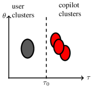
Figure 4: Illustration of an unsupervised clustering using the a priori information in the delay domain.

In a supervised scheme, ${\mathsf{Clst}}$ has access to an “oracle” provided by higher communication layers, which can be exploited to perform adaptive clustering. In brief, ${\mathsf{Clst}}$ starts from an initial clustering and refines it iteratively using the oracle response until a good partition of $\gamma(\theta,\tau)$ into ${\gamma_{{\mathtt{d}}}}(\theta,\tau)$ and ${\gamma_{{\mathtt{c}}{\mathtt{o}}}}(\theta,\tau)$ is obtained. A simple example of this is illustrated in Fig. 5. In this example, $\gamma(\theta,\tau)$ consists of one signal cluster and two CPU  clusters, where for simplicity we have assumed that these clusters are non-overlapping. The ${\mathsf{Clst}}$ starts with the obvious initialization ${\gamma_{{\mathtt{d}}}}(\theta,\tau)=\gamma(\theta,\tau)$, i.e., that there is no contamination (left figure in Fig. 5). Based on this assumption, it estimates the channel vector on all the subcarriers (using the channel interpolation scheme proposed in the following), and based on this channel estimation it attempts to decode the UL user data. In the presence of significant contamination, the effective Signal to Interference plus Noise Ratio (SINR) is degraded and some standard link layer control mechanism detects the data packet in error. This error detection mechanism can be exploited as an oracle for supervised learning. In the presence of a packet error, the ${\mathsf{Clst}}$ tries a different selection of the clusters (e.g., as in the center figure in Fig. 5). The process is repeated until the data packet is decoded correctly. Notice that in this case, although there is no guarantee that all the copilot interference be removed, we have the guarantee that it has been removed enough to decode the data, whenever this is possible. This means that the effective SINR for the desired user is large enough to achieve successful decoding. Of course, if no successful decoding is achieved after a fixed number of iterations, the packet is rejected, and the desired user is re-scheduled for transmission on a later slot. This is not different from a standard “packet failure” event, which is handled by retransmission or by any suitable upper layer protocol in a completely standard manner. Notice also that ${\mathsf{Clst}}$ learns the suitable clustering without any explicit feedback from the users since the whole process is performed entirely at the BS receiver on a single packet detection. Therefore, it does not involve any additional latency with respect to a standard massive MIMO system. Interestingly, in this example, the clusters corresponding to the CPUs have smaller propagation delays than the one corresponding to the desired user. As a result, the previously mentioned unsupervised algorithm, which only exploits the propagation delay of the users, would fail to identify the signal cluster. Such a situation arises, for example, in a cell-free massive MIMO system, where copilot interference may be particularly harmful [29, 30].

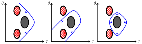
Figure 5: Illustration of a supervised clustering algorithm. In this figure, $\gamma(\theta,\tau)$ consists of one signal cluster (solid gray) plus two interference clusters (dashed) corresponding to two CPUs.

V-C Instantaneous Channel Estimation/Interpolation and Pilot Decontamination

Let ${\gamma_{{\mathtt{d}}}}(\theta,\tau)$ and ${\gamma_{{\mathtt{c}}{\mathtt{o}}}}(\theta,\tau)$ be the PSFs of the desired user and of the CPUs, obtained as described before. For channel decontamination and interpolation, we apply the MMSE smoothing filter (4) with “plug-in” covariance estimates given by ${\bf C}^{*}_{{\mathbb{h}}}=\int{\gamma_{{\mathtt{d}}}}(d\theta,d\tau){\mathbb{a}}(\theta,\tau){\mathbb{a}}(\theta,\tau)^{{\sf H}}$ for the desired user channel, and by ${\bf C}^{*}_{{\mathbb{i}}}=\int{\gamma_{{\mathtt{c}}{\mathtt{o}}}}(d\theta,d\tau){\mathbb{a}}(\theta,\tau){\mathbb{a}}(\theta,\tau)^{{\sf H}}$ for the superposition of the CPU  channels. The resulting plug-in channel estimator-interpolator is given by

$$\widehat{{\mathbb{h}}}_{s} =\hbox{\boldmath$\Sigma$}_{{\mathbb{h}}{\mathbb{x}}}{\bf C}^{-1}_{{\mathbb{x}}}{\mathbb{x}}_{s}\approx{\bf C}^{*}_{{\mathbb{h}}}{\mathbb{S}}_{s}^{{\sf H}}(\sigma^{2}{\bf I}_{mn}+{\mathbb{S}}_{s}({\bf C}^{*}_{{\mathbb{h}}}+{\bf C}^{*}_{{\mathbb{i}}}){\mathbb{S}}_{s}^{{\sf H}})^{-1}{\mathbb{x}}_{s},$$ (17)

where $\hbox{\boldmath$\Sigma$}_{{\mathbb{h}}{\mathbb{x}}}={\mathbb{E}}[{\mathbb{h}}_{s}{\mathbb{x}}_{s}^{{\sf H}}]$ denotes the cross covariance matrix of ${\mathbb{h}}_{s}$ and ${\mathbb{x}}_{s}$, and where ${\mathbb{x}}_{s}={\rm vec}({\bf X}_{s})$ is the UL pilot observation at time slot $s$. Under the condition that the estimated covariance matrices ${\bf C}^{*}_{\mathbb{h}}$ and ${\bf C}^{*}_{\mathbb{i}}$ are close to the true covariance matrices ${\bf C}_{\mathbb{h}}$ and ${\bf C}_{\mathbb{i}}$, the channel estimator in (17) is close to the ideal MMSE smoothing filter (4). Notice that in the absence of copilot interference (i.e., for ${\bf C}_{\mathbb{i}}={\bf 0}$) such MMSE smoothing filter implements the optimal channel interpolation in the antenna and frequency domain in the MMSE sense. In conventional implementations, “ad-hoc” channel interpolation techniques in the OFDM subcarrier domain are used in order to interpolate the unobserved columns (subcarriers) and rows (antennas) of the channel matrix ${\bf H}_{s}$ from the instantaneous noisy UL pilot observation ${\bf X}_{s}$ as given in (2). Typical schemes include simple piecewise constant, linear, or DFT-based (Sinc-shaped) interpolation (see [31, 32] and the refs. therein). The advantage of our proposed subspace estimation for pilot decontamination is that, as seen from (17), the channel vector ${\mathbb{h}}_{s}$ can be directly estimated from the sketch ${\mathbb{x}}_{s}$, thus, we obtain per-slot channel estimation/interpolation for free.

VI Low-complexity Channel Interpolation and Pilot Decontamination

Computing the $MN\times MN$ covariance matrices from the estimated PSF $\gamma(\theta,\tau)$ and performing the matrix multiplication for the MMSE estimation in (17), as proposed in the previous section, may result in a prohibitive complexity for typical massive MIMO systems (e.g., $M=128$ antennas and $N=128$ subcarriers). In this section, we propose two low-complexity algorithms to address this computational complexity issue. The first algorithm, explained in Section VI-A, uses a masking technique in the angle-delay domain, which yields a low-complexity approximation of the MMSE estimator proposed in (17). The second algorithm, stated in Section VI-B, has much lower complexity but, in order to guarantee to eliminate pilot contamination, requires a stronger angular separability condition as we will explain.

VI-A Interpolation and Pilot Decontamination by Masking

Let $\gamma(\theta,\tau)$ be the estimated PSF supported on the grid elements $(\theta_{l},\tau_{l})\in{\cal G}$ as in Section V-A. We define the mask ${\cal M}$ as follows

$${\cal M}:=\big{\{}(\theta_{l},\tau_{l}):\gamma(\theta_{l},\tau_{l})\geq\iota\big{\}},$$ (18)

where $\iota\in{\mathbb{R}}_{+}$ denotes a masking threshold in the angle-delay domain which selects only those grid elements with a significantly large received power. We assume that ${\cal M}={\cal M}^{\mathbb{h}}\cup{\cal M}^{\mathbb{i}}$ is decomposed into disjoint signal and CPU interference masks ${\cal M}^{\mathbb{h}}$ and ${\cal M}^{\mathbb{i}}$ with ${\cal M}^{\mathbb{h}}\cap{\cal M}^{\mathbb{i}}=\emptyset$ via the clustering algorithm ${\mathsf{Clst}}$. For the case of supervised clustering, ${\mathsf{Clst}}$ changes the masks ${\cal M}^{\mathbb{h}}$ and ${\cal M}^{\mathbb{i}}$ in each iteration, while keeping their union equal to ${\cal M}$ as in (18), until it finds a good estimate of the true signal cluster, e.g., when the packet decoding is successful as described before.

Let ${{\bf S}_{s}^{\mathtt{a}}}$ and ${{\bf S}_{s}^{\mathtt{f}}}$ be the antenna and frequency sampling matrices at slot $s$. We apply joint interpolation and pilot decontamination as follows. We find an estimate of the channel matrix ${\bf H}_{s}$ denoted by ${\bf P}$ and an estimate of copilot interference denoted by ${\bf Q}$ via minimizing $\|{\bf X}_{s}-{{\bf S}_{s}^{\mathtt{a}}}({\bf P}+{\bf Q}){{{\bf S}_{s}^{\mathtt{f}}}}^{{\sf H}}\|$, where ${\bf X}_{s}={{\bf S}_{s}^{\mathtt{a}}}{\bf Y}_{s}{{{\bf S}_{s}^{\mathtt{f}}}}^{{\sf H}}$ denotes the subsampled observations at slot $s$ and where ${\bf Y}_{s}$ denotes the noisy contaminated received wideband signal. To do so, we impose the additional constraint that a significant amount of power of ${\bf P}$ and ${\bf Q}$ be concentrated in the mask ${\cal M}^{\mathbb{h}}$ and ${\cal M}^{\mathbb{i}}$ in the angle-delay domain, respectively. We denote by ${{\mathtt{F}}^{\text{ovs}}}:{\mathbb{C}}^{M\times N}\to{\mathbb{C}}^{G^{\theta}\times G^{\tau}}$ the oversampled 2D DFT and by ${{\mathtt{F}}}:{\mathbb{C}}^{G^{\theta}\times G^{\tau}}\to{\mathbb{C}}^{G^{\theta}\times G^{\tau}}$ the usual 2D DFT in dimension $G^{\theta}\times G^{\tau}$, where $\frac{G^{\theta}}{M}$ and $\frac{G^{\tau}}{N}$ denote the oversampling factors in the angle and delay domain respectively. Note that for an $M\times N$ matrix ${\bf H}$, we have ${{\mathtt{F}}^{\text{ovs}}}({\bf H})={{\mathtt{F}}}({\bf H}^{\text{ovs}})$ where ${\bf H}^{\text{ovs}}$ denotes a $G^{\theta}\times G^{\tau}$ matrix that has ${\bf H}$ in its up-left corner and is zero elsewhere. This follows from the well-known property of DFT, where an oversampling in one domain can be obtained by zero-padding in the corresponding transform domain. For simplicity, we assume that ${{\mathtt{F}}}$ is normalized such that it is an isometry preserving the matrix Frobenius norm, i.e., $\|{{\mathtt{F}}}({\bf L})\|=\|{\bf L}\|$ for any $G^{\theta}\times G^{\tau}$ matrix ${\bf L}$. We define the following cost function for ${\bf P}$ and ${\bf Q}$

$$c({\bf P},{\bf Q}) =\frac{1}{2}\|{\bf X}_{s}-{{\bf S}_{s}^{\mathtt{a}}}({\bf P}+{\bf Q}){{{\bf S}_{s}^{\mathtt{f}}}}^{{\sf H}}\|^{2}+\mathbb{I}_{{\cal M}^{\mathbb{h}}}({{\mathtt{F}}^{\text{ovs}}}({\bf P}))+\mathbb{I}_{{\cal M}^{\mathbb{i}}}({{\mathtt{F}}^{\text{ovs}}}({\bf Q}))$$ (19)

where $\mathbb{I}_{{\cal M}^{\mathbb{h}}},\mathbb{I}_{{\cal M}^{\mathbb{i}}}:{\mathbb{C}}^{G^{\theta}\times G^{\tau}}\to{\mathbb{R}}_{+}\cup\{+\infty\}$ are convex regularizers penalizing those nonzero coefficients of their arguments not belonging to the masks ${\cal M}^{\mathbb{h}}$ and ${\cal M}^{\mathbb{i}}$ respectively. A simple regularizer is the indicator function of a mask ${\cal D}$, given by:

$$\mathbb{I}_{{\cal D}}({\bf K}):=\left\{\begin{array}[]{ll}\infty&\text{ if }{\bf K}({\sim{\cal D}})\neq{\bf 0},\\ 0&\text{otherwise,}\end{array}\right.$$ (22)

where ${\bf K}({\sim{\cal D}})$ denotes those elements of the matrix ${\bf K}$ not belonging to ${\cal D}$. The cost function in (19) is convex and its globally optimal solution $({\bf P}^{*},{\bf Q}^{*})$ can be found via convex optimization techniques. The optimal solution ${\bf P}^{*}$ of (19) is an estimate of the decontaminated channel matrix ${\bf H}_{s}$. In the presence of antenna and frequency sampling, this technique (masking and optimization) provides an interpolation scheme to recover the whole channel matrix from its subsamples. In Appendix A, we propose a low-complexity algorithm for solving (19) using Alternating Direction Method of Multipliers (ADMM), which estimates/interpolates the decontaminated channel matrix with a complexity $O(G\log_{2}(G))$, where $G=G^{\theta}G^{\tau}$ denotes the total number of points in the grid ${\cal G}$. This provides a low-complexity implementation of the MMSE smoothing filter proposed in Section V-C.

VI-B Low-complexity Pilot Decontamination under the Angular Separability Condition

In this section, we explain another pilot decontamination algorithm that has much lower complexity than the MMSE estimator (17) proposed in Section V-C but, to eliminate pilot contamination, it requires a stronger condition that marginal PSF ${\gamma_{{\mathtt{d}}}}(\theta)$ and ${\gamma_{{\mathtt{c}}{\mathtt{o}}}}(\theta)$ of the user and its CPUs have approximately disjoint supports in the angular domain, where we define ${\gamma_{{\mathtt{d}}}}(\theta)=\int_{0}^{\Delta\tau_{\max}}{\gamma_{{\mathtt{d}}}}(\theta,d\tau)$ with a similar definition holding for ${\gamma_{{\mathtt{c}}{\mathtt{o}}}}(\theta)$. This is illustrated qualitatively in Fig. 6.

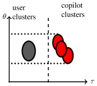
(a) Overlapping.

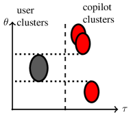
(b) Non-overlapping.

Figure 6: Illustration of two extremes of angular overlap of the PSF of the desired user ${\gamma_{{\mathtt{d}}}}(\theta)$ and that of its CPUs ${\gamma_{{\mathtt{c}}{\mathtt{o}}}}(\theta)$: Overlapping (a) and Non-overlapping (b).

Notice that the separability of ${\gamma_{{\mathtt{d}}}}(\theta,\tau)$ and ${\gamma_{{\mathtt{c}}{\mathtt{o}}}}(\theta,\tau)$ in the joint angle-delay domain is still necessary to successfully decompose (cluster) the PSF $\gamma(\theta,\tau)$ into its signal and interference components ${\gamma_{{\mathtt{d}}}}(\theta,\tau)$ and ${\gamma_{{\mathtt{c}}{\mathtt{o}}}}(\theta,\tau)$.

Let ${\bf H}_{s}$ and ${\bf H}_{s,j},j\in{\cal K}$, be the channel matrices of a user and of its CPUs, and let ${{\bf E}}_{s}=\sum_{j\in{\cal K}}{\bf H}_{s,j}$ be the channel matrix of CPU interference. Let ${\bf C}_{{\mathbb{h}}}^{*}=\int{\gamma_{{\mathtt{d}}}}(d\theta d\tau){\mathbb{a}}(\theta,\tau){\mathbb{a}}(\theta,\tau)^{{\sf H}}$ be the estimated covariance matrix of the channel vector ${\mathbb{h}}_{s}={\rm vec}({\bf H}_{s})$ from the estimated PSF ${\gamma_{{\mathtt{d}}}}(\theta,\tau)$ obtained from the clustering. It is not difficult to check that ${\bf C}^{*}_{{\mathbb{h}}}$ is a block-Toeplitz matrix, which implies that every column ${\bf h}_{s}[\omega]$ of ${\bf H}_{s}$ is an $M$-dim Gaussian vector with a covariance matrix well approximated by ${\bf C}^{*}_{{\bf h}}=\int{\gamma_{{\mathtt{d}}}}(d\theta){\bf a}(\theta){\bf a}(\theta)^{{\sf H}}$, where ${\bf C}^{*}_{{\bf h}}$ is an $M\times M$ Toeplitz matrix and corresponds to the diagonal block of ${\bf C}^{*}_{{\mathbb{h}}}$. Similarly, every column ${{\bf e}}_{s}[\omega]$ of the CPU  interference ${{\bf E}}_{s}$ is an $M$-dim Gaussian vectors with a Toeplitz covariance matrix given by ${\bf C}^{*}_{{{\bf e}}}=\int{\gamma_{{\mathtt{c}}{\mathtt{o}}}}(d\theta){\bf a}(\theta){\bf a}(\theta)^{{\sf H}}$. Let ${\bf Y}_{s}={\bf H}_{s}+{{\bf E}}_{s}+{\bf Z}_{s}$ be the received noisy and pilot contaminated signal. For simplicity, we first assume that there is no antenna or frequency sampling and ${\bf Y}_{s}$ is fully available. We consider the following suboptimal scheme for pilot decontamination: Instead of estimating the whole channel matrix ${\bf H}_{s}$ from ${\bf Y}_{s}$, as we did for the MMSE estimation in Section V-C, we estimate each column ${\bf h}_{s}[\omega]$ of ${\bf H}_{s}$ from the corresponding column ${\bf y}_{s}[\omega]$ of ${\bf Y}_{s}$ individually. Since ${\bf y}_{s}[\omega]={\bf h}_{s}[\omega]+{{\bf e}}_{s}[\omega]+{\bf z}_{s}[\omega]$, this is a standard problem of estimating a Gaussian $M$-dim vector ${\bf h}_{s}[\omega]$ in an additive colored Gaussian noise ${{\bf e}}_{s}[\omega]+{\bf z}_{s}[\omega]$. The resulting MMSE estimator can be simply written as

$$\widehat{{\bf h}}_{s}[\omega] =\hbox{\boldmath$\Sigma$}_{{\bf h}{\bf y}}{\bf C}_{{\bf y}}^{-1}{\bf y}_{s}[\omega]\approx{\bf C}_{{\bf h}}^{*}\left(\sigma^{2}{\bf I}_{M}+{\bf C}_{\bf h}^{*}+{\bf C}_{{\bf e}}^{*}\right)^{-1}{\bf y}_{s}[\omega],$$ (23)

where $\hbox{\boldmath$\Sigma$}_{{\bf h}{\bf y}}={\mathbb{E}}[{\bf h}_{s}[\omega]{\bf y}_{s}[\omega]^{{\sf H}}]$ denotes the cross correlation matrix of ${\bf h}_{s}[\omega]$ and ${\bf y}_{s}[\omega]$. It is seen that the MMSE estimator is an $M\times M$ linear operator, which requires computing the inverse of an $M\times M$ Toeplitz matrix rather than an $MN\times MN$ block-Toeplitz matrix, as was necessary for the joint MMSE estimator in Section V-C. More importantly, since the spatial correlation of the channel is invariant with the subcarrier index $\omega$ due to the stationarity in the frequency domain, the linear estimator is the same for all the columns of the channel matrix, thus, it needs to be computed only once.

If in addition there is an antenna sampling via an operator ${\bf S}_{s}^{\mathtt{a}}$, letting ${\bf x}_{s}[\omega]={\bf S}_{s}^{\mathtt{a}}{\bf y}_{s}[\omega]$ to be the $m$-dim sketch at subcarrier $\omega$ after antenna sampling, the MMSE estimator of ${\bf h}_{s}[\omega]$ from ${\bf x}_{s}[\omega]$ takes on the form

$$\widehat{{\bf h}}_{s}[\omega] =\hbox{\boldmath$\Sigma$}_{{\bf h}{\bf x}}{\bf C}_{{\bf x}}^{-1}{\bf x}_{s}[\omega]\approx{\bf C}_{{\bf h}}^{*}{{\bf S}_{s}^{\mathtt{a}}}^{{\sf H}}\left(\sigma^{2}{\bf I}_{m}+{\bf S}_{s}^{\mathtt{a}}({\bf C}_{\bf h}^{*}+{\bf C}_{{\bf e}}^{*}){{\bf S}_{s}^{\mathtt{a}}}^{{\sf H}}\right)^{-1}{\bf x}_{s}[\omega].$$ (24)

When the channel matrices of several users are learned over the same OFDM symbol, only a subset of columns of ${\bf Y}_{s}$ is observed for each user. In such a case, we apply the column-wise pilot-decontamination in (23) or (24) to estimate the corresponding columns of ${\bf H}_{s}$. Then, we apply traditional channel interpolation methods to reconstruct the remaining columns of ${\bf H}_{s}$ from the estimated ones (e.g., via piecewise constant, linear, or DFT-based interpolation techniques [31, 32]). The proposed suboptimal pilot decontamination reduces the implementation complexity considerably. However, the drawback is that in contrast with ${\gamma_{{\mathtt{d}}}}(\theta,\tau)$ and ${\gamma_{{\mathtt{c}}{\mathtt{o}}}}(\theta,\tau)$, which are usually well-separable in the joint angle-delay domain, ${\gamma_{{\mathtt{d}}}}(\theta)$ and ${\gamma_{{\mathtt{c}}{\mathtt{o}}}}(\theta)$ might generally overlap in the angle domain. In such a case, the dominant subspaces of ${\bf C}_{{\bf h}}$ and ${\bf C}_{{{\bf e}}}$ will be highly overlapping, and the suboptimal MMSE will eliminate a significant fraction of the power of the columns of the channel matrix ${\bf H}_{s}$ lying in the interference subspace ${\bf C}_{{{\bf e}}}$, which results in a poor design of the final beamforming matrix.

In practice, since the number of CPUs is typically small, if the users have a limited angular support and are quite randomly distributed inside the cell, there is a high chance that the effective overlap between $\gamma_{s}(\theta)$ and $\gamma_{i}(\theta)$ be quite negligible for most users. Another way to make $\gamma_{s}(\theta)$ and $\gamma_{i}(\theta)$ non-overlapping consists of shuffling the pilots assigned to the active users across the whole system as proposed in [9]. This is illustrated qualitatively in Fig. 7, where by re-allocating the pilot of the users of interest the BS can induce angular separation with respect to the CPUs. Pilot-shuffling requires some coordination among neighboring BSs inside the system. In [9, 12], it is assumed that the PSFs or the covariance matrices ${\bf C}_{\bf h}$ and ${\bf C}_{{\bf e}}$ of all the users and their CPUs are available. In contrast, in this paper we estimate the PSFs by using wideband pilots and exploiting the sparsity in the angle-delay domain, and identify the signal and interference PSFs by applying suitable clustering algorithms. Hence, our scheme to identify ${\bf C}_{\bf h}$ and ${\bf C}_{{\bf e}}$ directly from the pilot data can be seen as an enabler for the coordinated pilot shuffling scheme in [9] and the pilot decontamination in [12].

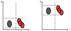
(a) Before Shuffling the Pilots.

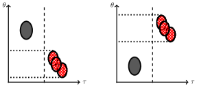
(b) After Shuffling the Pilots.

Figure 7: Separability in the angle domain via shuffling the pilots among the users: Before shuffling the pilots (a) and after shuffling the pilots (b).

VII Simulation Results

In this section, we assess the performance of our proposed pilot decontamination and channel interpolation algorithm via numerical simulations.

VII-A Cellular Geometry and Antenna Model

We consider a cellular system consisting of hexagonal cells of radius $R_{\text{cell}}=1.5$ Km and a maximum tolerable delay spread of $\Delta\tau_{\max}=\frac{2R_{\text{cell}}}{c_{0}}=10$ $\mu$s. For simulations, we assume the transmit/receive power decays with a power-loss exponent $\eta=3.2$ (for large cells), where the SNR before beamforming for a user located at a distance $r$ from the BS is given by $\text{SNR}(r)=\frac{\text{SNR}_{\max}}{1+(\frac{r}{r_{0}})^{\eta}}$, where $r_{0}=500$ m, and where $\text{SNR}_{\max}$ is selected such that the SNR before beamforming for a user located at the cell boundary is $\text{SNR}_{\min}=5$ dB. We repeat the simulations for $\eta=2$ (small cells) to intensify the effect of interference, especially copilot interference, received from the users in adjacent cells. We normalize the SNR such that the SNR before beamforming for a user close to the BS remains the same in both scenarios.

We assume that each hexagonal cell is divided into $3$ sectors as illustrated in Fig. 8. The BS uses a ULA with $M$ antennas to serve the users inside each sector, thus, the whole BS transmitter consists of $3$ ULAs (one per sector). The ULAs are well isolated in the RF domain such that each ULA only receives the signal of the users lying in its 120 deg angular span $[-\theta_{\max},\theta_{\max}]$ with $\theta_{\max}=60$ degrees.

(a)

(b)

Figure 8: Pilot distribution for a system with PR3 (a) and PR1 (b), with copilot sectors highlighted in gray.

VII-B Scattering Model

We consider a one-ring scattering model for the user signal, where the transmitted signal from a user in the UL is reflected by a ring a scatterers located around the user with a radius of $R_{\text{one-ring}}=150$ meters. We assume that all the scatterers contribute equally in terms of scattering power to the channel vector of the user observed at the BS. Thus, all the users have an equal delay-span of $\frac{2R_{\text{one-ring}}}{c_{0}}=1$ $\mu$s but different angular spreads depending on their distance from the BS.

VII-C Physical Channel Model and OFDM Parameters

We use a physical channel model similar to LTE (Long-Term Evolution) as in [1]. We consider a slot of duration $T_{s}=0.532$ ms and decide arbitrarily to send $7$ OFDM symbols over each slot, thus, each OFDM symbol has a total duration of $\frac{T_{s}}{7}=76$ $\mu$s and an effective duration $T_{u}=\frac{T_{s}}{7}-\Delta\tau_{\max}=66$ $\mu$s after removing the CP, corresponding to a frequency spacing of $\Delta f=\frac{1}{T_{u}}=15$ KHz between subcarriers. We take a bandwidth of $W=2$ MHz with a frequency guard-band of $80$ KHz, thus, the total number of subcarriers in each ODFM symbol is given by $N=\frac{1.92\text{ MHz}}{15\text{ KHz}}=128$.

Assuming a coherence bandwidth of $\Delta f_{c}=150$ KHz, the number of subcarriers in each coherence sub-block (see Fig. 2) is $D^{\text{c}}_{\text{OFDM}}=\Delta f_{c}T_{u}\approx 10$. Thus, the wideband channel matrix of $10$ users can be simultaneously learned over an individual training OFDM symbol, which enforces a subcarrier sampling ratio $\frac{1}{10}$, i.e., we can sample only $n=\lfloor\frac{N}{10}\rfloor=12$ out of $N=128$ subcarriers of an OFDM symbol. We devote $3$ OFDM symbols to channel estimation, where we are able to learn the channel matrix and, hence, serve up to $D_{\text{p}}=30$ users on a single TDD slot, consistently with the LTE-TDD standard.

We simulate a sectorized cellular system with each cell consisting of $3$ sectors numbered $\{1,2,3\}$ as illustrated in Fig. 8. We consider a system with a Pilot Reuse 3 (PR3) as illustrated in Fig. 8a, in which the set of $D^{\text{c}}_{\text{p}}=30$ orthogonal pilots are shared among $3$ sectors such that sectors with similar numbers use identical set of pilots consisting of $10$ mutually orthogonal pilot sequences (i.e., $K=10$ served users in each sector), and groups of 3 adjacent sectors with different indices (1,2,3) use collectively all the 30 orthogonal pilot sequences. We also consider a system with a Pilot Reuse 1 (PR1) as illustrated in Fig. 8b, in which all the $30$ orthogonal pilot sequences are simultaneously used in all the sectors, thus, each sector can serve up to $K=30$ users.

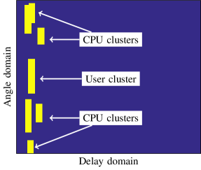
(a)

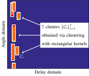
(b)

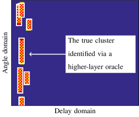
(c)

Figure 9: Illustration of the supervised clustering in one-ring model. Fig. (a) illustrates the estimated angle-delay PSF, where it is not initially known which cluster belongs to the desired user. Fig. (b) denotes a simple clustering of the estimated PSF into $7$ rectangular kernels ($1$ for the user and $6$ for its CPUs). Fig. (c) illustrates the identification of the true signal cluster via a higher-layer communication protocol.

VII-D Clustering Algorithm

Since in PR3 illustrated in Fig. 8a users and their CPUs are well-separated in the delay domain, we apply an unsupervised clustering in the delay domain as in Fig. 4 with a delay threshold $\tau_{0}=\frac{R_{\text{cell}}}{c_{0}}$. In particular, we set ${\gamma_{{\mathtt{d}}}}(\theta,\tau)=\gamma(\theta,\tau){\bf 1}_{\{(\theta,\tau)\in{\cal C}^{\text{PR3}}_{\mathtt{d}}\}}$ and ${\gamma_{{\mathtt{c}}{\mathtt{o}}}}(\theta,\tau)=\gamma(\theta,\tau){\bf 1}_{\{(\theta,\tau)\notin{\cal C}^{\text{PR3}}_{\mathtt{d}}\}}$, where ${\cal C}^{\text{PR3}}_{\mathtt{d}}$ in the desired signal cluster given by ${\cal C}^{\text{PR3}}_{\mathtt{d}}=\Big{\{}(\theta,\tau):\tau\leq\tau_{0}\Big{\}}$. For PR1, the users and their CPUs are not generally separable in the delay domain (see, e.g., Fig. 9a). Here, we need to apply a supervised clustering algorithm to identify the desired user cluster. In the one-ring scattering model we consider for the simulations, the PSF of each user consists of a single angle-delay cluster (bubble). Since the number of CPUs is at most $6$, we cluster the estimated PSF into $7$ rectangular-shaped clusters illustrated in Fig. 9b. This separates approximately the clusters corresponding to the user and its CPUs but does not specify yet which cluster corresponds to the user. To identify the user cluster, we use the “oracle” provided from a higher communication layer with the following scheme. After receiving the noisy contaminated channel sketch ${\mathbb{x}}_{s}$ during a pilot transmission slot, we obtain estimates $\widehat{{\mathbb{h}}}_{s}^{i}$, $i=1,2,\dots,7$, of the decontaminated channel vector of the user by treating the $i$-th cluster as the true signal cluster and the rest as CPU clusters, and applying our proposed channel interpolation algorithm in Section VI-A. During the data transmission phase, after receiving the whole ODFM symbol, we decode the received data by beamforming along the columns of the channel matrix corresponding to $\widehat{{\mathbb{h}}}_{s}^{i}$, $i=1,\dots,7$, once at a time, where we assume that there is a higher-layer oracle that selects the $\widehat{{\mathbb{h}}}_{s}^{i}$ and the corresponding cluster that results in a successful decoding of the user data as illustrated in Fig. 9c.

VII-E Uplink Pilot Decontamination

For simulations, we focus on pilot decontamination in an UL scenario, where we focus on the users belonging to Sector $1$ as in Fig. 8. The dominant copilot interference for each one of those users in the UL comes from its $2$ nearest neighbor CPUs in PR3 and from its $6$ nearest neighbor CPUs in PR1. For each user, the BS learns the superposition of the channel vector of that user plus those of its CPUs. Note that due to the orthogonality of the pilots, during the UL training phase, there is only copilot interference but no interference from the other users. During the data transmission phase (UL or DL), however, there is a coherent interference from CPUs and a noncoherent interference from all the other users. Notice also that CPUs coming from non-nearest neighbor copilot sectors are received at significantly lower power and at larger delays. Such signals are not guaranteed to be eliminated by the proposed method since the OFDM model fails due to inter-block interference (MPCs whose delays go beyond the CP interval). Nevertheless, the effect of non-nearest neighbors copilot contamination is very small.

VII-F Antenna Sampling and Wideband Pilot Sketches

We consider an antenna sampling ratio of $0.25$, where over each OFDM training symbol only $m=0.25M$ of the whole number of antennas $M$ are sampled. We assume that the sampling pattern is completely random and changes i.i.d. over time. We take a window of size ${\sf w}=100$ of sketches across ${\sf w}$ time slots to estimate the channel geometry of each user, where we assume that the channel matrices inside the window are i.i.d. since they belong to different slots (coherence times). As the whole observation takes ${\sf w}T_{s}=50$ ms, we can safely assume that the channel geometry remains invariant over the whole window.

VII-G Pilot Decontamination, Channel Interpolation, and Beamforming

After estimating the PSF of all the users, we apply the clustering algorithm explained in Section VII-D and the masking technique as in (18) to obtain the signal mask ${\cal M}^{{\mathbb{h}}}$ and the interference mask ${\cal M}^{{\mathbb{i}}}$ for each user, which we use for the rest of the time. We next simulate the communication phase, where each CB consists of a training phase to estimate the instantaneous channel vectors of the user and a data-transmission phase to send data to these users via spatial beamforming. In each training slot $s$, after receiving a sketch of the channel vector of each user, we apply the low-complexity channel interpolation and decontamination algorithm in Section VI-A to estimate the full channel vector of the user. For simplicity of comparison with the contaminated case, we assume no antenna sampling is applied during a training slot. We denote the decontaminated channel vectors of the $K$ users at the reference BS by $\{\widehat{{\mathbb{h}}}_{k}\}_{k=1}^{K}$ and the corresponding channel matrices by $\{\widehat{{\bf H}}_{k}\}_{k=1}^{K}$, where for simplicity we dropped the dependence on the data transmission slot $s$. We also assume that the noise power $\sigma^{2}$ in each antenna is available at the BS.

In PR3, we apply the MMSE beamforming for each user in the UL, where the normalized beamforming vector for a user $u\in[K]$ at subcarrier $\omega$ is given by by ${\bf g}_{k}[\omega]=\frac{{\bf v}_{k}[\omega]}{\|{\bf v}_{k}[\omega]\|}$, where

$${\bf v}_{k}[\omega]=\Big{(}\sigma^{2}{\bf I}_{M}+\sum_{k^{\prime}}\widehat{{\bf h}}_{k^{\prime}}[\omega]{\widehat{{\bf h}}_{k^{\prime}}[\omega]}^{{\sf H}}\Big{)}^{-1}\widehat{{\bf h}}_{k}[\omega],$$ (25)

where $\widehat{{\bf h}}_{k}[\omega]$ denotes the decontaminated and interpolated channel vector of the user $k$ at subcarrier $\omega$. Due to the sectorization, the BS in Sector 1 not only receives the pilot signal of its users but can also listen to the pilot signal of the users in adjacent sectors since they are using disjoint set of pilots. Thus, the summation over $k^{\prime}$ in (25) is taken over all the users inside the sector as well as the users in adjacent sectors. For PR1, we use a simple conjugate beamforming [1] given by ${\bf g}_{k}[\omega]=\frac{\widehat{{\bf h}}_{k}[\omega]}{\|\widehat{{\bf h}}_{k}[\omega]\|}$. We compare the performance of our method with the case where no pilot decontamination is applied. We assume that in such a case also $1$ out of $10$ of columns of channel matrix of each user is observed during a training slot. We apply DFT interpolation to interpolate the unobserved columns of the channel matrix of each user and repeat similar steps, as in the decontaminated case, to design the beamforming vectors. We define the SINR of the channel of the user $k\in[K]$ at subcarrier $\omega$ by

$${\mathsf{sinr}}_{k}[\omega]=\frac{\Big{|}{\bf g}_{k}[\omega]^{{\sf H}}{\bf h}_{k}[\omega]\Big{|}^{2}}{\sigma^{2}+\sum_{k^{\prime}\neq k}\Big{|}{\bf g}_{k}[\omega]^{{\sf H}}{\bf h}_{k^{\prime}}[\omega]\Big{|}^{2}},$$ (26)

where the summation is taken over all the users $k^{\prime}\neq k$ inside the sector as well as all other users in adjacent cells who lie in the angular span of the ULA of Sector $1$ and create interference. Assuming perfect channel state information after beamforming, the instantaneous spectral efficiency of user $k$ is given by $R_{k}=\frac{1}{N}\sum_{\omega\in[N]}\log_{2}(1+{\mathsf{sinr}}_{k}[\omega])$. We denote the achievable sum-rate in bit/s/Hz of all the users in Sector $1$ by $R=\sum_{k\in[K]}R_{k}$, where $R$ is a random variable depending on the instantaneous realizations of the channel vectors of all the users.

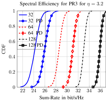
(a)

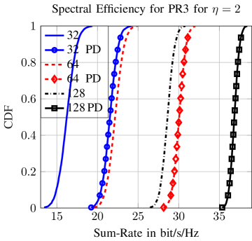
(b)

Figure 10: CDF of Spectral Efficiency (Sum-Rate) in bit/s/Hz for different number of BS antennas $M\in\{32,64,128\}$ for PR3 with $\eta=3.2$ (a) and $\eta=2$ (b). The curves with marks and with the legend “PD” illustrate the CDF after pilot decontamination. All the plots are averaged over $N_{\text{geom}}=30$ random user locations in the system.

VII-H Achievable Performance and Comparison with the State of the Art

1) PR3: Fig. 10 illustrates the Cumulative Distribution Function (CDF) $F_{R}(r)$ of the achievable spectral efficiency $R$ in bit/s/Hz before and after pilot decontamination. We average the CDFs over $N_{\text{geom}}=30$ independent realizations of the geometry of users across the system. For each geometry realization, we run the simulations for different number of BS antennas $M\in\{32,64,128\}$. We also consider two different scenarios for two different power-loss exponents $\eta\in\{3.2,2\}$ as explained in Section VII-A. It is seen that for $\eta=3.2$ and for practical numbers of BS antennas $M\in\{32,64,128\}$ pilot decontamination improves the spectral efficiency by $10\%-20\%$ for PR3, where the resulting gain increases by increasing the number of BS antennas $M$. For $\eta=2$, on the other hand, our proposed scheme results in a dramatic gain in spectral efficiency.

(a)

(b)

Figure 11: CDF of Spectral Efficiency in bit/s/Hz of a specific user close to the cell boundary for different number of BS antennas $M\in\{128,256\}$ in a system with PR1 for $\eta=3.2$ (a) and $\eta=2$ (b). The curves with marks illustrate the CDF after pilot decontamination: our algorithm with the legend “PD” and the algorithm in [16] with the legend “PD [16]”. All the plots are averaged over $N_{\text{geom}}=30$ random user locations in the system.

2) PR1: We repeat the simulations for PR1. In this case, to pinpoint the effect of pilot contamination, rather than calculating the sum-rate averaged over all the random locations of the users, we focus on an “edge” user randomly located on the cell boundary. We expect that the spectral efficiency of such a user be affected considerably by the pilot contamination from the neighboring CPUs. As illustrated in Fig. 9, pilot decontamination for edge users in PR1 requires a supervised clustering in the angle-delay domain. Fig. 11 illustrates the simulation results. We compare the performance of our algorithm with the one proposed in [16]. In [16], the support of the MPCs of the contaminated channel vector of the user is estimated by devoting all the subcarriers in an OFDM symbol to an individual user and projecting the whole channel matrix in the 2D FFT basis. The support of the desired user is identified and separated from that of its CPUs by taking the intersection of the support obtained over several slots, where in each slot the pilots are shuffled such that the desired user collides with different CPUs at each slot. The rationale behind this idea is that in this way the support of the MPCs of the desired user remains constant over the sequence of slots, while that of the CPUs changes from slot to slot. Therefore, taking the intersection of the estimated supports over the slots should yield the MPCs of the desired user. However, in doing so, the intersection will also exclude the MPCs of the desired user that over the sequence of slots experience a deep fade, since these will be missed on some slots, and therefore will not be contained in the intersection. As a matter of fact, with time-selective fading as in our realistic setting, we could verify that the method of [16] dramatically underestimates the MPCs of the desired user.

In contrast, our proposed subspace estimation with supervised clustering is much robust to small-scale fading variations, performs much better in the presence of overlapping clusters (e.g., when a user and it CPUs have common clusters), and does not require pilot shuffling among the neighboring cells. Also, compared with [16], in our proposed scheme only a fraction (e.g., $\frac{1}{10}$) of the subcarriers in an OFDM symbol are devoted as pilot to each user, so the channel state of several users (e.g., $10$ users) can be simultaneously estimated over an individual OFDM symbol, thus, much better multiplexing gain. Notice that using the whole set of $N$ OFDM subcarriers for UL pilots is essential to the method of [16] since otherwise there is not enough resolution in the delay domain. This is because [16] makes use of simple linear projections, while our scheme estimates the PSF using the advanced $l_{2,1}$-regularized least squares minimization described in Section IV.

Our simulation results in Fig. 11 consider the rate CDF of a single edge user randomly located near the cell boundary, thus, they do not reflect the additional multiplexing gain resulting from using a reduced pilot dimension $n\ll N$. For the simulations, we assume that the total number of users is the same in both scenarios ($30$ users per sector), where similar to PR3 we average the achievable spectral efficiency of this specific edge user over $N_{\text{geom}}=30$ independent realizations of the geometry of all the users across the whole system. From Fig. 11, it is seen that the gain in spectral efficiency obtained by our method is much more than the one proposed in [16]. In particular, the resulting gain scales much better with the number of BS antennas.

VIII Conclusions

In this paper, we presented a novel scheme to eliminate the effect of pilot contamination on the performance of a massive MIMO wireless cellular system. We proposed a low-complexity algorithm that uses the pilot signal received from each user inside a window containing several time slots to obtain an estimate of the angle-delay power spread function (PSF) of each user contaminated channel vectors. We used the key idea, already exploited in various ways in the recent massive MIMO literature, that the channel vectors of each user consist of sparse MPCs in the angle-delay domain. We exploited this underlying sparsity to estimate the angle-delay PSF of each user by sampling only a small subset of antennas and, more importantly, by transmitting pilots across only a subset of subcarriers compatible with LTE-TDD without incurring any pilot overhead. We proposed clustering algorithms to decompose the estimated PSF of each user into its signal and copilot interference part. We exploited this decomposition to decontaminate the channel vector of each user in the next coherence blocks. Through Monte Carlo simulation, we demonstrated the effectiveness of the proposed pilot-decontamination scheme for practical scenarios with practical user geometries, reasonable number of BS antennas $M\in\{32,64,128,256\}$, and realistic fading channel statistics as in [1]. We also compared our proposed method with the competitive scheme [16] and illustrated that our method provides much better performance in terms of multiplexing gain, pilot decontamination efficiency, and scaling performance with the number of BS antennas.

Appendix A Low-complexity Interpolation using ADMM

Consider the following cost function as in (19):

$$c({\bf P},{\bf Q}) =\frac{1}{2}\|{\bf X}_{s}-{{\bf S}_{s}^{\mathtt{a}}}({\bf P}+{\bf Q}){{{\bf S}_{s}^{\mathtt{f}}}}^{{\sf H}}\|^{2}+\mathbb{I}_{{\cal M}^{\mathbb{h}}}({{\mathtt{F}}^{\text{ovs}}}({\bf P}))+\mathbb{I}_{{\cal M}^{\mathbb{i}}}({{\mathtt{F}}^{\text{ovs}}}({\bf Q})).$$ (27)

In this section, we assume that the convex regularizers $\mathbb{I}_{{\cal M}^{\mathbb{h}}}$ and $\mathbb{I}_{{\cal M}^{\mathbb{i}}}$ are the indicator functions of ${{\cal M}^{\mathbb{h}}}$ and ${{\cal M}^{\mathbb{i}}}$ defined similarly to (22). We first introduce the auxiliary variables ${\bf P}_{\mathtt{f}}={{\mathtt{F}}^{\text{ovs}}}({\bf P})$ and ${\bf Q}_{\mathtt{f}}={{\mathtt{F}}^{\text{ovs}}}({\bf Q})$ of dimension $G^{\theta}\times G^{\tau}$ and define

$$c({\bf P},{\bf Q},{\bf P}_{\mathtt{f}},{\bf Q}_{\mathtt{f}}) =\frac{1}{2}\|{\bf X}_{s}-{{\bf S}_{s}^{\mathtt{a}}}({\bf P}+{\bf Q}){{{\bf S}_{s}^{\mathtt{f}}}}^{{\sf H}}\|^{2}+\mathbb{I}_{{\cal M}^{\mathbb{h}}}({\bf P}_{\mathtt{f}})+\mathbb{I}_{{\cal M}^{\mathbb{i}}}({\bf Q}_{\mathtt{f}}).$$ (28)

Thus, minimizing $c({\bf P},{\bf Q})$ in (27) can be equivalently written as minimizing $c({\bf P},{\bf Q},{\bf P}_{\mathtt{f}},{\bf Q}_{\mathtt{f}})$ under the additional linear constraints ${\bf P}_{\mathtt{f}}={{\mathtt{F}}^{\text{ovs}}}({\bf P}),{\bf Q}_{\mathtt{f}}={{\mathtt{F}}^{\text{ovs}}}({\bf Q})$, which is still a convex optimization problem. We use Alternating Direction Method of Multipliers (ADMM) to solve this optimization problem. We introduce the Lagrange variables $\hbox{\boldmath$\Lambda$}_{\mathtt{p}}$ and $\hbox{\boldmath$\Lambda$}_{\mathtt{q}}$ of dimension $G^{\theta}\times G^{\tau}$ and the augmented Lagrangian function

$${\mathscr{L}} =\frac{1}{2}\|{\bf X}_{s}-{{\bf S}_{s}^{\mathtt{a}}}({\bf P}+{\bf Q}){{{\bf S}_{s}^{\mathtt{f}}}}^{{\sf H}}\|^{2}+\mathbb{I}_{{\cal M}^{\mathbb{h}}}({\bf P}_{\mathtt{f}})+\mathbb{I}_{{\cal M}^{\mathbb{i}}}({\bf Q}_{\mathtt{f}})$$

$$+{\langle\hbox{\boldmath$\Lambda$}_{\mathtt{p}},{\bf P}_{\mathtt{f}}-{{\mathtt{F}}^{\text{ovs}}}({\bf P})\rangle}_{\mathbb{R}}+{\langle\hbox{\boldmath$\Lambda$}_{\mathtt{q}},{\bf Q}_{\mathtt{f}}-{{\mathtt{F}}^{\text{ovs}}}({\bf Q})\rangle}_{\mathbb{R}}$$

$$+\frac{\upsilon}{2}\|{\bf P}_{\mathtt{f}}-{{\mathtt{F}}^{\text{ovs}}}({\bf P})\|^{2}+\frac{\upsilon}{2}\|{\bf Q}_{\mathtt{f}}-{{\mathtt{F}}^{\text{ovs}}}({\bf Q})\|^{2},$$ (29)

where $\upsilon\in{\mathbb{R}}_{+}$ is the ADMM parameter to be set. The ADMM iteration can be written as follows:

$$({\bf P}^{k+1},{\bf Q}^{k+1}) =\mathop{\rm arg\,min}_{{\bf P},{\bf Q}}{\mathscr{L}}({\bf P},{\bf Q},{\bf P}_{\mathtt{f}}^{k},{\bf Q}_{\mathtt{f}}^{k},\hbox{\boldmath$\Lambda$}_{\mathtt{p}}^{k},\hbox{\boldmath$\Lambda$}_{\mathtt{q}}^{k}),$$ (30)

$$({\bf P}_{\mathtt{f}}^{k+1},{\bf Q}_{\mathtt{f}}^{k+1}) =\mathop{\rm arg\,min}_{{\bf P}_{\mathtt{f}},{\bf Q}_{\mathtt{f}}}{\mathscr{L}}({\bf P}^{k+1},{\bf Q}^{k+1},{\bf P}_{\mathtt{f}},{\bf Q}_{\mathtt{f}},\hbox{\boldmath$\Lambda$}_{\mathtt{p}}^{k},\hbox{\boldmath$\Lambda$}_{\mathtt{q}}^{k}),$$ (31)

$$\hbox{\boldmath$\Lambda$}_{\mathtt{p}}^{k+1} =\hbox{\boldmath$\Lambda$}_{\mathtt{p}}^{k}+\upsilon({\bf P}_{\mathtt{f}}^{k+1}-{{\mathtt{F}}^{\text{ovs}}}({\bf P}^{k+1})),$$ (32)

$$\hbox{\boldmath$\Lambda$}_{\mathtt{q}}^{k+1} =\hbox{\boldmath$\Lambda$}_{\mathtt{q}}^{k}+\upsilon({\bf Q}_{\mathtt{f}}^{k+1}-{{\mathtt{F}}^{\text{ovs}}}({\bf Q}^{k+1})),$$ (33)

Updating ${\bf P}^{k+1},{\bf Q}^{k+1}$: Using the vectorization and denoting by ${\mathbb{p}}={\rm vec}({\bf P})$, ${\mathbb{q}}={\rm vec}({\bf Q})$, ${\mathbb{x}}_{s}={\rm vec}({\bf X}_{s})$, ${\bf P}_{\mathtt{t}}={{\mathtt{F}}^{\text{ovs}}}^{-1}({\bf P}_{\mathtt{f}}^{k}+\frac{1}{\upsilon}\hbox{\boldmath$\Lambda$}^{k}_{\mathtt{p}})$, ${\bf Q}_{\mathtt{t}}={{\mathtt{F}}^{\text{ovs}}}^{-1}({\bf Q}^{k}_{\mathtt{f}}+\frac{1}{\upsilon}\hbox{\boldmath$\Lambda$}^{k}_{\mathtt{p}})$, ${\mathbb{p}}_{\mathtt{t}}={\rm vec}({\bf P}_{\mathtt{t}}({\text{$1$\,:\,$M$}},{\text{$1$\,:\,$N$}}))$, ${\mathbb{q}}_{\mathtt{t}}={\rm vec}({\bf Q}_{\mathtt{t}}({\text{$1$\,:\,$M$}},{\text{$1$\,:\,$N$}}))$, we can write (30) as the following cost function to be minimized for $MN\times 1$ vectors ${\mathbb{p}}$ and ${\mathbb{q}}$:

$$\frac{1}{2}\|{\mathbb{x}}_{s}-{\mathbb{S}}_{s}({\mathbb{p}}+{\mathbb{q}})\|^{2}+\frac{\upsilon}{2}\|{\mathbb{p}}-{\mathbb{p}}_{\mathtt{t}}\|^{2}+\frac{\upsilon}{2}\|{\mathbb{q}}-{\mathbb{q}}_{\mathtt{t}}\|^{2},$$ (34)

where ${\mathbb{S}}_{s}={\bf S}_{s}^{\mathtt{f}}\otimes{\bf S}_{s}^{\mathtt{a}}$ denotes the sampling operator at slot $s$. The optimal solution of (34) is given by

$${\mathbb{p}}^{k+1} ={\mathbb{p}}_{\mathtt{t}}+\frac{\check{{\mathbb{x}}}_{s}}{\upsilon}+{\mathscr{S}}_{s}\big{(}2{\mathscr{S}}_{s}+\upsilon{\mathscr{I}}\big{)}^{-1}({\mathbb{p}}_{\mathtt{t}}+{\mathbb{q}}_{\mathtt{t}}+\frac{2\check{{\mathbb{x}}}_{s}}{\upsilon}),$$ (35)

$${\mathbb{q}}^{k+1} ={\mathbb{q}}_{\mathtt{t}}+\frac{\check{{\mathbb{x}}}_{s}}{\upsilon}+{\mathscr{S}}_{s}\big{(}2{\mathscr{S}}_{s}+\upsilon{\mathscr{I}}\big{)}^{-1}({\mathbb{p}}_{\mathtt{t}}+{\mathbb{q}}_{\mathtt{t}}+\frac{2\check{{\mathbb{x}}}_{s}}{\upsilon}),$$ (36)

where $\check{{\mathbb{x}}}_{s}={\mathbb{S}}_{s}^{{\sf H}}{\mathbb{x}}_{s}$, ${\mathscr{S}}_{s}={\mathbb{S}}_{s}^{{\sf H}}{\mathbb{S}}_{s}$, and where ${\mathscr{I}}={\bf I}_{MN}$ denotes the identity matrix of order $MN$. Since in this paper we always use 0-1 antenna and frequency sampling matrices, (35) and (36) can be further simplified. Using the properties of the ${\rm vec}$ operator, we have that

$${\mathscr{S}}_{s}={\mathbb{S}}_{s}^{{\sf H}}{\mathbb{S}}_{s}=({{\bf S}_{s}^{\mathtt{f}}}^{{\sf H}}\otimes{{\bf S}_{s}^{\mathtt{a}}}^{{\sf H}})({{\bf S}_{s}^{\mathtt{f}}}\otimes{{\bf S}_{s}^{\mathtt{a}}})=({{\bf S}_{s}^{\mathtt{f}}}^{{\sf H}}{{\bf S}_{s}^{\mathtt{f}}})\otimes({{\bf S}_{s}^{\mathtt{a}}}^{{\sf H}}{{\bf S}_{s}^{\mathtt{a}}}).$$ (37)

Note that, due to 0-1 sampling, ${{\bf S}_{s}^{\mathtt{f}}}^{{\sf H}}{{\bf S}_{s}^{\mathtt{f}}}$ and ${{\bf S}_{s}^{\mathtt{a}}}^{{\sf H}}{{\bf S}_{s}^{\mathtt{a}}}$ are diagonal matrices of dimension $M\times M$ and $N\times N$ with 1s in the diagonal elements corresponding to the index sets ${\cal I}_{s}^{\mathtt{f}}$ and ${\cal I}_{s}^{\mathtt{a}}$ and $0$ elsewhere, where ${\cal I}_{s}^{\mathtt{a}}\subseteq[M]$ and ${\cal I}_{s}^{\mathtt{f}}\subseteq[N]$ denote the indices of antennas and subcarriers sampled at slot $s$ as explained in Section III-C. This implies that ${\mathscr{S}}_{s}$ is a 0-1 diagonal matrix of dimension $MN\times MN$ where the locations of 1s in the diagonal is given as in (11) by

$${\cal I}_{s}:=\{M(c_{s}^{\mathtt{f}}-1)+c_{s}^{\mathtt{a}}:\ \ c_{s}^{\mathtt{f}}\in{\cal I}_{s}^{\mathtt{f}},\ c_{s}^{\mathtt{a}}\in{\cal I}_{s}^{\mathtt{a}}\}\subseteq[MN].$$ (38)

As a result, the matrix ${\mathscr{S}}_{s}\big{(}2{\mathscr{S}}_{s}+\upsilon{\mathscr{I}}\big{)}^{-1}$ in (35) and (36) is a diagonal matrix with a value $\frac{1}{\upsilon+2}$ at the diagonal elements belonging to ${\cal I}_{s}$ and $0$ elsewhere. Moreover, no matrix-vector multiplication is needed for computing $\check{{\mathbb{x}}}_{s}={\mathbb{S}}_{s}^{{\sf H}}{\mathbb{x}}_{s}$ since $\check{{\mathbb{x}}}_{s}$ is simply given by an $MN\times 1$ vector that contains the components of ${\mathbb{x}}_{s}$ in the indices corresponding to ${\cal I}_{s}$ and is $0$ elsewhere. This implies that ${\mathbb{p}}^{k+1}$ and ${\mathbb{q}}^{k+1}$ can be easily computed from (35) and (36), from which we obtain ${\bf P}^{k+1}$ and ${\bf Q}^{k+1}$ via inverse ${\rm vec}$ operation. The whole computational complexity of this step comes from calculating ${\mathbb{p}}_{\mathtt{t}}$ and ${\mathbb{q}}_{\mathtt{t}}$, which requires $O(G\log_{2}(G))$ operations where $G=G^{\theta}G^{\tau}$ denotes the grid size as before.

Updating ${\bf P}_{\mathtt{f}}^{k+1},{\bf Q}_{\mathtt{f}}^{k+1}$: We first derive the update equation for ${\bf P}_{\mathtt{f}}^{k+1}$ in (31). To find ${\bf P}_{\mathtt{f}}^{k+1}$, we need to optimize the following function with respect to ${\bf P}_{\mathtt{f}}$:

$$\frac{\upsilon}{2}\|{\bf P}_{\mathtt{f}}+\frac{1}{\upsilon}\hbox{\boldmath$\Lambda$}^{k}_{\mathtt{p}}-{{\mathtt{F}}^{\text{ovs}}}({\bf P}^{k+1})\|^{2}+{\mathbb{I}}_{{\cal M}^{\mathbb{h}}}({\bf P}_{\mathtt{f}}).$$ (39)

The optimal solution of (39) is given by setting ${\bf P}^{k+1}_{\mathtt{f}}$ equal to ${{\mathtt{F}}^{\text{ovs}}}({\bf P}^{k+1})-\frac{1}{\upsilon}\hbox{\boldmath$\Lambda$}^{k}_{\mathtt{p}}$ at those elements belonging to the mask ${\cal M}^{\mathbb{h}}$ while setting the remaining components equal to zero. Similarly, ${\bf Q}^{k+1}_{\mathtt{f}}$ is given by ${{\mathtt{F}}^{\text{ovs}}}({\bf Q}^{k+1})-\frac{1}{\upsilon}\hbox{\boldmath$\Lambda$}^{k}_{\mathtt{q}}$ over the mask ${\cal M}^{\mathbb{i}}$ and zero elsewhere. The whole computational complexity of this step is also $O(G\log_{2}(G))$ for computing ${{\mathtt{F}}^{\text{ovs}}}({\bf P}^{k+1})$ and ${{\mathtt{F}}^{\text{ovs}}}({\bf Q}^{k+1})$. Overall, the computational complexity of each ADMM iteration is $O(G\log_{2}(G))$.

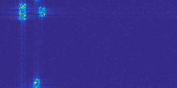
(a) 2D DFT of received signal.

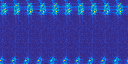
(b) After $1$ ADMM iteration.

(c) After $2$ ADMM iterations.

(d) After $3$ ADMM iterations.

Figure 12: Illustration of ADMM algorithm for a user in a system with PR3. Fig. (a) illustrates the 2D DFT of noisy contaminated channel vector of the user in the angle (vertical) and delay (horizontal) domain. The channel vector consists of a desired signal cluster along with $2$ interfering copilot clusters. Fig. (b) show the 2D DFT after the first iteration, which also shows the appearance of aliasing pattern (with $10$ replicas) due to subsampling (by a factor $10$) in the frequency (subcarrier) domain. From Subfig. (c) and (d), it is seen that the algorithm reconstructs the true channel matrix quite fast.

A-A Simulation Results

Fig. 12 illustrates the performance our proposed ADMM algorithm in decontaminating/interpolating the channel vector of the user. For simulation, we consider a user inside a cellular system with PR3 as illustrated in Fig. 8. The Subfig. (a) in Fig. 12 shows the 2D DFT of the received noisy and contaminated channel vector in the angle-delay domain. It is seen that the received signal contains a desired signal cluster with smaller propagation delay and two copilot clusters with larger delays. It is seen that our proposed masking technique in Section VI-A along with the ADMM implementation reconstructs the decontaminated channel matrix quite fast. Interestingly, in this example, one of the copilot clusters overlaps with the signal cluster in the angle domain, thus, the column-wise decontamination of the channel matrix, as proposed in Section VI-B, will not be effective.

References

- [1] T. L. Marzetta, “Noncooperative cellular wireless with unlimited numbers of base station antennas,” IEEE Trans. on Wireless Commun., vol. 9, no. 11, pp. 3590–3600, Nov. 2010.
- [2] C. Shepard, H. Yu, N. Anand, E. Li, T. Marzetta, R. Yang, and L. Zhong, “Argos: Practical many-antenna base stations,” in Proceedings of the 18th Annual International Conference on Mobile Computing and Networking. ACM, 2012, pp. 53–64.
- [3] E. Larsson, O. Edfors, F. Tufvesson, and T. Marzetta, “Massive mimo for next generation wireless systems,” IEEE Communications Magazine, vol. 52, no. 2, pp. 186–195, 2014.
- [4] L. You, X. Gao, A. L. Swindlehurst, and W. Zhong, “Channel acquisition for massive mimo-ofdm with adjustable phase shift pilots.” IEEE Trans. Signal Processing, vol. 64, no. 6, pp. 1461–1476, 2016.
- [5] J. Jose, A. Ashikhmin, T. L. Marzetta, and S. Vishwanath, “Pilot contamination and precoding in multi-cell tdd systems,” IEEE Transactions on Wireless Communications, vol. 10, no. 8, pp. 2640–2651, 2011.
- [6] H. Huh, G. Caire, H. Papadopoulos, and S. Ramprashad, “Achieving massive MIMO spectral efficiency with a not-so-large number of antennas,” IEEE Trans. on Wireless Commun., vol. 11, no. 9, pp. 3226–3239, 2012.
- [7] J. Hoydis, S. Ten Brink, and M. Debbah, “Massive mimo in the ul/dl of cellular networks: How many antennas do we need?” IEEE J. on Sel. Areas on Commun. (JSAC), vol. 31, no. 2, pp. 160–171, 2013.
- [8] E. Björnson, E. G. Larsson, and M. Debbah, “Massive mimo for maximal spectral efficiency: How many users and pilots should be allocated?” IEEE Transactions on Wireless Communications, vol. 15, no. 2, pp. 1293–1308, 2016.
- [9] H. Yin, D. Gesbert, M. Filippou, and Y. Liu, “A coordinated approach to channel estimation in large-scale multiple-antenna systems,” IEEE Journal on Selected Areas in Communications, vol. 31, no. 2, pp. 264–273, 2013.
- [10] A. Adhikary, J. Nam, J.-Y. Ahn, and G. Caire, “Joint spatial division and multiplexingÑthe large-scale array regime,” IEEE Trans. on Inform. Theory, vol. 59, no. 10, pp. 6441–6463, 2013.
- [11] J. Nam, A. Adhikary, J.-Y. Ahn, and G. Caire, “Joint spatial division and multiplexing: Opportunistic beamforming, user grouping and simplified downlink scheduling,” IEEE J. of Sel. Topics in Sig. Proc. (JSTSP), vol. 8, no. 5, pp. 876–890, 2014.
- [12] E. Björnson, J. Hoydis, and L. Sanguinetti, “Pilot contamination is not a fundamental asymptotic limitation in massive mimo,” arXiv preprint arXiv:1611.09152, 2016.
- [13] R. R. Muller, L. Cottatellucci, and M. Vehkapera, “Blind pilot decontamination,” IEEE Journal of Selected Topics in Signal Processing, vol. 8, no. 5, pp. 773–786, 2014.
- [14] H. Yin, L. Cottatellucci, D. Gesbert, R. R. Muller, and G. He, “Robust pilot decontamination based on joint angle and power domain discrimination,” IEEE Transactions on Signal Processing, vol. 64, no. 11, pp. 2990–3003, 2016.
- [15] L. Li, A. Ashikhmin, and T. Marzetta, “Pilot contamination precoding for interference reduction in large scale antenna systems,” in 2013 51st Annual Allerton Conference on Communication, Control, and Computing (Allerton). IEEE, 2013, pp. 226–232.
- [16] Z. Chen and C. Yang, “Pilot decontamination in wideband massive mimo systems by exploiting channel sparsity,” IEEE Transactions on Wireless Communications, vol. 15, no. 7, pp. 5087–5100, 2016.
- [17] H. Holma and A. Toskala, LTE for UMTS: Evolution to LTE-advanced. John Wiley & Sons, 2011.
- [18] H. Shirani-Mehr and G. Caire, “Channel state feedback schemes for multiuser mimo-ofdm downlink,” IEEE Transactions on Communications, vol. 57, no. 9, 2009.
- [19] D. Tse and P. Viswanath, Fundamentals of wireless communication. Cambridge university press, 2005.
- [20] A. F. Molisch, Wireless communications. John Wiley & Sons, 2012, vol. 34.
- [21] L. Liu, C. Oestges, J. Poutanen, K. Haneda, P. Vainikainen, F. Quitin, F. Tufvesson, and P. Doncker, “The cost 2100 mimo channel model,” IEEE Wireless Communications, vol. 19, no. 6, pp. 92–99, 2012.
- [22] B. Clerckx and C. Oestges, MIMO Wireless Networks: Channels, Techniques and Standards for Multi-Antenna, Multi-User and Multi-Cell Systems. Academic Press, 2013.
- [23] K. Liu, V. Raghavan, and A. M. Sayeed, “Capacity scaling and spectral efficiency in wide-band correlated mimo channels,” IEEE Transactions on Information Theory, vol. 49, no. 10, pp. 2504–2526, 2003.
- [24] G. Auer, “3d mimo-ofdm channel estimation,” IEEE Transactions on Communications, vol. 60, no. 4, pp. 972–985, 2012.
- [25] B. H. Fleury, “First-and second-order characterization of direction dispersion and space selectivity in the radio channel,” IEEE Transactions on Information Theory, vol. 46, no. 6, pp. 2027–2044, 2000.
- [26] S. Haghighatshoar and G. Caire, “Massive mimo channel subspace estimation from low-dimensional projections,” IEEE Transactions on Signal Processing, vol. 65, no. 2, pp. 303–318, 2017.
- [27] ——, “Low-complexity massive mimo subspace estimation and tracking from low-dimensional projections,” arXiv preprint arXiv:1608.02477, 2016.
- [28] A. Nemirovski, “Efficient methods in convex programming,” 2005.
- [29] H. Q. Ngo, A. Ashikhmin, H. Yang, E. G. Larsson, and T. L. Marzetta, “Cell-free massive mimo: Uniformly great service for everyone,” in Signal Processing Advances in Wireless Communications (SPAWC), 2015 IEEE 16th International Workshop on. IEEE, 2015, pp. 201–205.
- [30] O. Y. Bursalioglu, C. Wang, H. Papadopoulos, and G. Caire, “Rrh based massive mimo with “on the fly” pilot contamination control,” in Communications (ICC), 2016 IEEE International Conference on. IEEE, 2016, pp. 1–7.
- [31] J.-W. Choi and Y.-H. Lee, “Optimum pilot pattern for channel estimation in ofdm systems,” IEEE Transactions on Wireless Communications, vol. 4, no. 5, pp. 2083–2088, 2005.
- [32] A. Hutter, R. Hasholzner, and J. Hammerschmidt, “Channel estimation for mobile ofdm systems,” in Vehicular Technology Conference, 1999. VTC 1999-Fall. IEEE VTS 50th, vol. 1. IEEE, 1999, pp. 305–309.