17 The Diffusion of Humans and Cultures in the Course of the Spread of Farming

Keywords: Cultural diffusion; demic diffusion; farming; Neolithic

17.1 Introduction

The most profound change in the relationship between humans and their environment was the introduction of agriculture and pastoralism. With this millennia lasting economic shift from simple food acquisition to complex food production humankind paved the way for its grand transitional process from mobile groups to sedentary villages, towns and ultimately cities, and from egalitarian bands to chiefdoms and lastly states. Given this enormous historic impetus, Gordon Childe many years ago coined the term “Neolithic Revolution” [1].

The first experiments began with the end of the Glacial period about 10000 years ago in the so called Fertile Crescent [2]. They were followed by other endeavors in various locations both in the Americas and in Afroeurasia. Today farming has spread to all but the most secluded or marginal environments of the planet [3]. Cultivation of plants and animals on the global scale appears to have changed energy and material flows—like greenhouse gas emissions—so fundamentally, that the term “early anthropocene” is considered for the era following the Mid-Holocene [4].

Figure 17.1: Overview of the study area and the archaeologically visible expansion of farming.

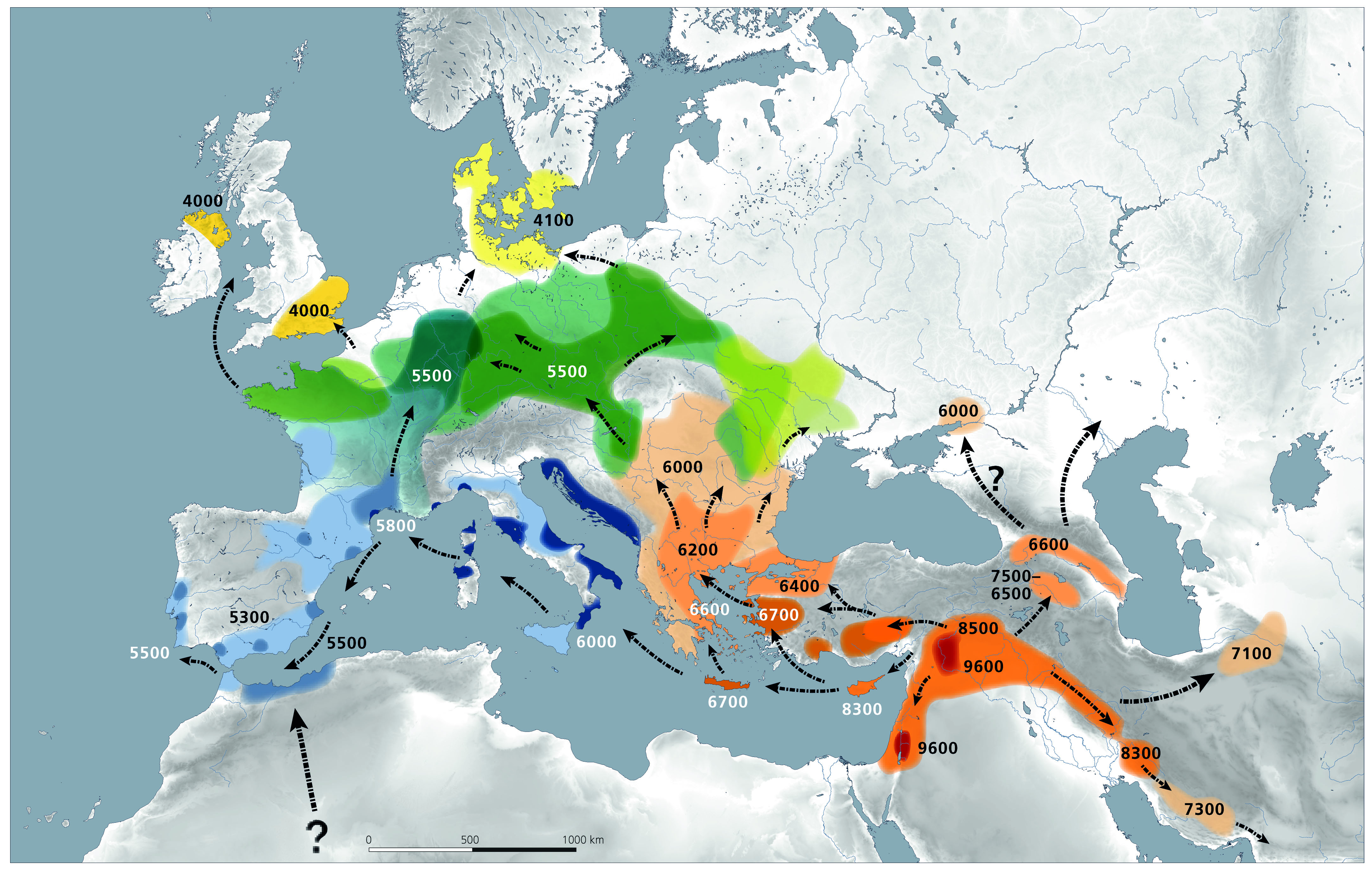
Possible reasons for the emergence of farming during the relatively confined period between the Early and Mid-Holocene in locations independent of each other are continuously being debated [2] [5] [6]. Once these inventions were in place, they immediately become visible in the archeological and paleoenvironmental records. From then on we can trace the spatial expansion of the newly domesticated plants and animals, the spatial expansion of a life style based on these domesticates, and the induced changes in land cover [7] [8]. From this empirically derived data the characteristic condensed map of the spread of farming into western Eurasia is produced (Figure 17.1).

The local changes introduced spatial differences in knowledge, labor, technology, materials, population density, and—more indirectly—social structure and political organization, amongst others [9] [10]. Consequently, the dynamics occurring along such spatial gradients may be modeled as a diffusive process. In Chapter 2, Fick’s first law was introduced, which describes that the average flux across a spatial boundary is proportional to the difference of concentration across this boundary (Chapter 2, Eq. 2.6). Each of the local inventions would then spread outward from its respective point of origin. Indeed, these spatiotemporal gradients have been observed in ceramics [1], radiocarbon dates [7] [11], domesticates [12] [13], land use change [14] [15], and the genetic composition of paleopopulations [16] [17] [18] [19].

For an understanding of the expansion process, it appears appropriate to apply a diffusive model. Broadly, these numerical modeling approaches can be categorized in correlative, continuous and discrete. Common to all approaches is the comparison to collections of radiocarbon data that show the apparent wave of advance of the transition to farming. However, these data sets differ in entry density and data quality. Often they disregard local and regional specifics and research gaps, or dating uncertainties. Thus, most of these data bases may only be used on a very general, broad scale. One of the pitfalls of using irregularly spaced or irregularly documented radiocarbon data becomes evident from the map generated by Fort (this volume, Chapter 16): while the general east-west and south-north trends become evident, some areas appear as having undergone anomalously early transitions to farming. This may be due to faulty entries into the data base or regional problems with radiocarbon dating, if not unnoticed or undocumented laboratory mistakes.

Correlative models compare the timing of the transition (or other archeologically visible frontier) with the distance from one or more points of origin. These are among the earliest models proposed, such as those by Clark [7] or by Ammerman [20]. These models have been used to roughly estimate the front propagation speed of the introduction of agriculture into Europe, and the original speed of around 1 km per year has not been substantially refined until today.

Continuous models predict at each location within the specified domain the transition time as the solution of a differential equation, mostly of a Fisher–Skellam type, in relation to the distance from one or more points of origin. Often this distance is not only the geometric distance but also factors in geography, topography and even ease of migration. The prediction from the continuous model is compared to the archeologically visible frontier [21]. This is the approach taken by Fort (this volume, Chapter 16) who compares the wave-front propagation of different models for the transition from a hunting and gathering economy to a farming economy in Europe with the spatiotemporal pattern of the earliest radiocarbon dates locally associated with farming.

Discrete models Discrete models are realized as agent-based models (see also Chapter 2.5), with geographic areas (or their populations) representing agents, and rules that describe the interaction, especially the diffusion properties, between them. They also predict for each geographic area the transition time, but not as an analytic, but rather as an emergent property of the system. We here introduce as an example the discrete agent-based and gradient-adaptive model the Global Land Use and technological Evolution Simulator (GLUES).

17.2 Agent-based gradient-adaptive model GLUES

Figure 17.2: Regions constituting the set of agents in the simulation (shown for Western Eurasia and North Africa) in 685 globally distributed regions)

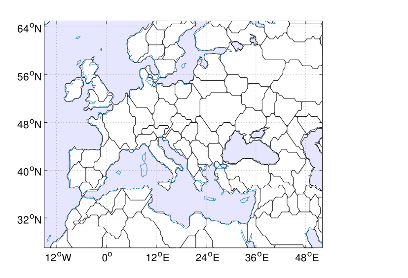
We employ the Global Land Use and technological Evolution Simulator (GLUES [22])–a numerical model of prehistoric innovation, demography, and subsistence economy based on interacting geographic populations as agents and gradient adaptive trait dynamics to describe local evolution. There are currently 685 regions representing the “cells” of agent-based models (Figure 17.2), together with interaction rules that describe diffusion of people, material and information between these regions. The agent is the population living within a region, and its state is described by its density and three characteristic population-average trait that evolve towards optimal local growth rate.

This numerical model is able to hindcast the regional transitions to agropastoralism and the diffusion of people and innovations across the world for the time span between approximately 8000 BCE (before the common era) and 1500 CE. It has been successfully compared to radiocarbon data for Europe [22], Eastern North America [23], and South Asia [24].

Regions are generated from ecozone clusters that have been derived to represent homogeneous net primary productivity ($E_{\mathrm{NPP}}$) based on a 3000 BCE 1^∘ $\times$ 1^∘ paleoproductivity estimate; this estimate was derived from a climatologically downscaled dynamic paleovegetation simulation [25]. By using $E_{\mathrm{NPP}}$, many of the environmental factors taken into account by other expansion or predictive models, such as altitude, latitude, rainfall, or temperature [12] [26] are implicitly considered.

17.2.1 Local characteristic variables

In each agent population, the mathematical model resolves the change over time of population density and three characteristic—meaning important—population-averaged sociocultural traits $X\in\left\{T,N,C\right\}$: technology $T$, share of agropastoral activities $C$, and economic diversity $N$. They are interpreted as follows:

1. Technology $T$ is a trait which describes the efficiency for enhancing biological growth rates, or diminishing mortality. It is represented by the efficiency of food procurement—related to both foraging and farming—and improvements in health care. In particular, technology as a model describes the availability of tools, weapons, and transport or storage facilities, and includes institutional aspects related to work organization and knowledge management. These are often synergistic: the technical and societal skill of writing as a means for cultural storage and administration, with the latter acting as an organizational lubricant for food procurement and its optimal allocation in space and among social groups;

2. Economic diversity $N$ resolves the number of different agropastoral economies available to a regional population. This trait is closely tied to regional vegetation resources and climate constraints. A larger economic diversity offering different niches for agricultural or pastoral practices enhances the reliability of subsistence and the efficacy in exploiting heterogeneous landscapes.

3. A third model variable $C$ represents the share of farming and herding activities, encompassing both animal husbandry and plant cultivation. It describes the allocation of energy, time, or manpower to agropastoralism with respect to the total food sector; this is the only variable that is directly comparable to data from the archeological record.

Characteristic trait	Symbol	Quantification	Typical range
Technology efficiency	$T$	Factor of efficiency gain over Mesolithic	$0.9$–$15$
Economic diversity	$N$	Richness of economic agropastoral strategies	$0.1$–$8$
Agropastoral share	$C$	Fraction of activities in agropastoralism	$0$–$1$

Table 17.1: Characteristic traits used in the Gradient Adaptive Dynamics formulation of GLUES; a full table of symbols used is available as Table 17.2.

17.2.2 Adaptive dynamics

The adaptive coevolution of the food production system $\{T,N,C\}$ and population density $P$ follow the conceptual model that was, e.g, proposed by Boserup [27]: “The close relationship which exists today between population density and food production system is the result of two long-existing processes of adaptation. On the one hand, population density has adapted to the natural conditions for food production []; on the other hand, food supply systems have adapted to changes in population density.”

Mathematically, this conceptual model is implemented in the Gradient Adaptive Dynamics (GAD) approach: Whenever traits can be related to growth rate, then an approach known as adaptive dynamics can be applied to generate the equations for the temporal change of traits, the so-called evolution equations. This adaptive dynamics was introduced by Metz [28] and goes back to earlier work by Fisher in the 1930s [29] and the field of genetics. When genetically encoded traits influence the fitness of individuals, that gene’s prevalence in a population changes. Adaptive dynamics describes the change of the probability of the trait in the population by considering its mutation rate and its fitness gradient, i.e., the marginal benefit of changes in the trait for the (reproductive) fitness of the individual.

To ecological systems, this metaphor was first applied in 1996 [30], and to cultural traits in 2003 [25]; in this translation, the genetically motivated term mutation rate was replaced by the ecologically observable variability of a trait. Because many traits are usually involved in (socio)ecological applications (here $T,N,C$), the term Gradient Adaptive Dynamics was introduced to emphasize the usage of the growth-rate gradient of the vector of traits.

17.2.2.1 Aggregation

Gradient Adaptive Dynamics describes the evolution of one or more aggregated (population-average) characteristic traits. By definition, it requires variability within a population, and is thus suitable for the description of medium-size to large populations.

In a local population $B$ composed of $n$ sub-population members $\iota\in\{1\ldots n\}$, each member with relative contribution $B_{\iota}/B$, characteristic traits $X_{\iota}$, and time-dependent environmental condition $E_{\iota}(t)$, has a relative growth rate $r_{\iota}$

$$r_{\iota}=\frac{1}{B}\cdot\frac{\mathrm{d}B_{\iota}}{\mathrm{d}t}=r_{\iota}\left(X_{\iota},E_{\iota}(t)\right).$$ (17.1)

This equation is often formulated in terms of the population density $P=B/A$, where $A$ is the area populated by $B$:

$$r_{\iota}=\frac{1}{P}\cdot\frac{\mathrm{d}P_{\iota}}{\mathrm{d}t} = r_{\iota}\left(X_{\iota},E_{\iota}(t)\right)$$ (17.2)

$$\textrm{and}\qquad\sum_{\iota}^{n}(P_{\iota}/P) = 1.$$

The mean of a quantity $X$ over all individuals $\iota$ is calculated as

$$\left\langle X\right\rangle=\sum_{\iota=1}^{n}\frac{X_{\iota}P_{\iota}}{P}.$$ (17.3)

The adaptive dynamics rooted in genetics assumes that mutation errors are only relevant at cell duplication, and not during cell growth. Translated to the ecological entity population this restriction enforces that all traits $X_{\iota}$ of a member of this population are stable during the lifetime of this member: $\frac{\mathrm{d}}{\mathrm{d}t}X_{\iota}=0$ for all $X_{\iota}$. Changes in the aggregated traits $\left\langle X\right\rangle$ are a result of frequency selection (the number of members carrying a specific characteristic trait increases or decreases as a result of selection) only.

17.2.2.2 Aggregated trait dynamics

Aggregation of Eq. 17.3, differentiation with respect to time, and considering $\frac{\mathrm{d}}{\mathrm{d}t}X_{\iota}=0$, gives

$$\frac{\mathrm{d}\left\langle X\right\rangle}{\mathrm{d}t} = \sum_{\iota=1}^{n}\frac{\partial{}\frac{X_{\iota}P_{\iota}}{P}}{\partial{}t}$$ (17.4)

$$= \left\langle X\cdot r(X)\right\rangle-\left\langle r(X)\right\rangle\cdot\left\langle X\right\rangle$$

Using a Taylor expansion of $r$ about $X=\left\langle X\right\rangle$, Eq. 17.4 can be reformulated in terms of the $(k+1)^{\mathrm{st}}$ central moment, of which the first summand is zero. Neglecting moments higher than $k=2$, the temporal change of $\left\langle X\right\rangle$ is

$$\frac{\mathrm{d}\left\langle X\right\rangle}{\mathrm{d}t}=\sigma_{X}^{2}\cdot\frac{\partial{}}{\partial{}X}r\left(\left\langle X\right\rangle\right)+v_{X}\sigma_{X}^{3}\frac{\partial{}^{2}}{\partial{}X^{2}}r\left(\left\langle X\right\rangle\right),$$ (17.5)

where $\sigma_{X}^{2}=\left\langle(X-\left\langle X\right\rangle)^{2}\right\rangle$ denotes the variance of $X$, and $v_{X}$ describes the skewness of $X$. Essentially, the population averaged value of a trait changes at a rate which is proportional to the marginal benefit (fitness) induced by trait changes on the growth rate $r$ evaluated at the mean characteristic trait value.

If the probability distribution of $X$ is known, the variance and skewness can be deduced; in other cases, variance and skewness have to be specified explicitly. The third moment may not be necessary in all cases and the approximation can be truncated after the second order term; if not, specific closure terms have to be derived. The use of the partial derivative on the right hand side of Equation (17.5) reflects that in all applications of gradient so far, non-local effects have been disregarded.

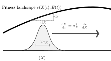
Leaving out the angular brackets around $X$ for better readability, and truncating at $k=1$, the gradient adaptive dynamics for trait $X$ is given by

$$\frac{\mathrm{d}X}{\mathrm{d}t}=\sigma_{X}^{2}\cdot\frac{\partial{}r(X)}{\partial{}X}$$ (17.6)

with $X\in\{T,N,C\}$. Equation (17.6) is visually shown in Figure 17.3.

Figure 17.3: The adaptive dynamics of a characteristic trait $X$ in a fitness landscape $r(X,E(t))$ is described by the width of the trait distribution ($\sigma_{X}$) and the marginal benefit that a small change in $X$ has on the growth rate $r$. Modified from [31].

17.2.3 Local population growth

Key to adaptive dynamics is the formulation of the growth rate as a function of all characteristic traits. Once this dependence is specified, the evolution equations for $X$ are generated automatically from Eq. 17.6.

Symbol	description	unit	typical range
$P$	population density	$\mathrm{km}^{-2}$	$>0$
$X$	growth-influencing trait		$>0$
$t$	time	a	9500–1000 BCE
$r$	specific growth rate	a-1
$E$	environmental constraints
$\left\langle\cdot\right\rangle$	mean / first moment of $\cdot$
$\sigma^{2}$	variance		$>0$
$\varsigma$	diffusion parameter		$>0$
$v$	skewness
$T$	technology trait		$>0$
$N$	economic trait		$>0$
$C$	labor allocation trait		$]0;1[$
$s$	subsistence intensity
$E_{\mathrm{TLI}}$	temperature limitation		$[0;1]$
$E_{\mathrm{FEP}}$	food extraction potential		$[0;1]$
$\omega$	administration parameter
$\gamma$	exploitation parameter
$\mu$	fertility rate	a-1
$\rho$	mortality rate	a-1

Table 17.2: Symbols and variables used in the text and equations (in order of appearance in text). A useful parameter set is $\mu=\rho=0.004$, $\omega=0.04$, $\gamma=0.12$, $\delta_{T}=0.025$, $\varsigma_{\mathrm{demic}}=0.002$, $\varsigma_{\mathrm{info}}=0.2$, $\delta_{N}=0.9$; a variable $\delta_{C}=C\cdot(1-C)$; and initial values for $P_{0}=0.01$, $T_{0}=1.0$, $N_{0}=0.8$, and $C_{0}=0.04$.

The relative growth rate $r$ of an agent population with density $P$ is the sum of gain and loss (often termed birth and death rates, respectively; see Table 1 for an overview of symbols used)

$$r=\mu\cdot\textrm{gain}-\rho\cdot\textrm{loss},$$ (17.7)

with loss and gain coefficients $\mu$ and $\rho$.

Out of several factors contributing to population gain, the Neolithic transition is foremost characterized by changes in subsistence intensity ($s$). Subsistence intensity describes a community’s effectiveness in generating consumable food and secondary products; this can be achieved based on an agricultural (with fractional activity $C$) and a hunting-gathering life style (with fractional activity $1-C$). The quantity ${s}$ is dimensionless and scaled such that a value of unity expresses the mean subsistence intensity of a hunter-gatherer society equipped with tools typical for the mature Mesolithic ($T=1,C\approx 0$).

$${s}=(1-C)\cdot\sqrt{T}+C\cdot N\cdot T\cdot E_{\mathrm{TLI}}$$ (17.8)

The agropastoral part of $s$ increases linearly with $N$ and with $T$: The more economies ($N$) there are, the better are sub-regional scaled niches utilized and the more reliable returns are generated when annual weather conditions are variable; the higher the technology level ($T$), the better the efficiency of using natural resources (by definition of $T$). While a variety of techniques can steeply increase harvests of domesticated species, analogous benefits for foraging productivity are less pronounced and justify a less than linear dependence of the hunting-gathering calorie procurement on $T$, such as a square root formulation.

We introduce an additional temperature constraint ($E_{\mathrm{TLI}}$) on agricultural productivity which considers that cold temperature could only moderately be overcome by Neolithic technologies. This limitation is unity at low latitudes and approaches zero at permafrost conditions.

The domestication process is represented by $N$, which is the number of realized agropastoral economies. We link $N$ to natural resources by expressing it as the fraction $f$ of potentially available economies ($E_{\mathrm{PAE}}$) by specifying $N=f\cdot E_{\mathrm{PAE}}$, where the latter corresponds to the richness in domesticable animal or plant species within a specific region.

To account for overexploitation of natural resources and productivity losses by societal organization, ${s}$ is multiplied by two terms representing those processes. $(E_{\mathrm{FEP}}-\gamma\sqrt{T}P)$ expresses the effects of overexploitation of natural resources $E_{\mathrm{FEP}}$ by increasing impact, calculated by the (scaled) product of technology and density ; organizational losses within a society are expressed by the term $(1-\omega\,T)$: as technology advances, more and more people neither farm nor hunt: Construction, maintenance, administration draw a small fraction $\omega$ of the workforce away from food-production. Gathering those gain terms, the growth rate equation is

$$r=\mu\cdot(E_{\mathrm{FEP}}-\gamma\sqrt{T}P)\cdot(1-\omega\,T)\cdot{s}-\textrm{loss}$$ (17.9)

The loss term takes a standard ecological form modeled on the crowding effect (also known as ecological capacity), and is thus proportional to $P$. It is mediated by technologies ($T$, with $T_{\mathrm{lit}}=12$), which mitigate, for example, losses due to disease. The full growth rate equation is then:

$$r=\mu\cdot(E_{\mathrm{FEP}}-\gamma\sqrt{T}P)\cdot(1-\omega\,T)\cdot{s}-\rho\cdot P\cdot\mathrm{e}^{-T/T_{\mathrm{lit}}},$$ (17.10)

17.2.4 Spatial diffusion model

Figure 17.4: Schematic representation of interregional exchange in GLUES.

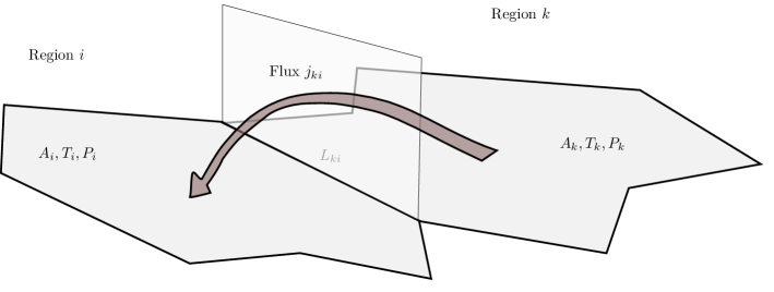
Information, material and people are diffused between regions with a flux modeled on Fickian diffusion (Chapter 2, eqs 2.6–2.9), modified for the discrete two-dimensional region arrangement and with a locally heterogeneous diffusion coefficient $D_{ik}$. The change of any characteristic trait $X_{i}$ in a region $i$ due to diffusion from/to all regions $k\in\mathcal{N}_{k}$ in its neighborhood $\mathcal{N}_{i}$ with neighbor distance $\Delta x_{ik}$ is

$${\frac{\Delta X_{i}}{\Delta t}}=\sum_{k\in\mathcal{N}_{i}}-j_{ik}/\Delta x_{ik},$$ (17.11)

with $j_{ik}=-D_{ik}\Delta X_{ik}/\Delta x_{ik}$ constituting the diffusive flux between $i$ and $k$ (Figure 17.4); This gives

$${\frac{\Delta X_{i}}{\Delta t}}=\sum_{k\in\mathcal{N}_{i}}D_{ik}\Delta X_{ik}\Delta x_{ik}^{-2}.$$ (17.12)

This equation can be reformulated [32] as

$${\frac{\Delta X_{i}}{\Delta t}}=\varsigma\sum_{k\in\mathcal{N}_{i}}f_{ik}\Delta X_{ik}$$ (17.13)

with $f_{ik}=j_{ik}\Delta x_{ik}^{-2}\varsigma^{-1}$, where $\varsigma$ is a global diffusion property characterizing the underlying process (see below) and $f_{ik}$ collects all regionally varying spatial and social diffusive aspects.

The social factor in the formulation of $f_{ik}$ is the difference between two regions’ influences , where influence is defined as the product of population density $P$ and technology $T$, scaled by the average influence of regions $i,k$. The geographic factor is the conductance between the two regions, which is constructed from the common boundary length $L_{ik}$ divided by the mean area of the regions $\sqrt{A_{i}A_{k}}$. Non-neighbour regions by definition have no common boundary, and hence have zero conductance; to connect across the Strait of Gibraltar, the English Channel, and the Bosporus, the respective conductances were calculated as if a narrow land bridge connected them. No additional account is made for increased conductivity along rivers [33], as the regional setup of the model is biased (through the use of $E_{\mathrm{NPP}}$ similarity clusters) toward elongating regions in the direction of rivers. Altitude and latitude effects are likewise implicitly accounted for by the $E_{\mathrm{NPP}}$ clustering in the region generation.

17.2.5 Three types of diffusion

Three types of diffusion are distinguished: (1) demic diffusion, i.e. the migration of people, (2) the hitchhiking of traits with migrants, and (3) cultural diffusion, i.e. the information exchange of characteristic traits.

Demic diffusion is the mass-balanced migration of people between different regions. The diffusion equation 17.13 is applied to the number of inhabitants $B_{i}=P_{i}A_{i}$ in each region $i$.

$$\left.\displaystyle{\frac{\mathrm{d}B_{i}}{\mathrm{d}t}}\right|_{\mathrm{demic}}=\begin{cases}\varsigma_{\mathrm{demic}}\sum_{j\in\mathcal{N}_{i}}f_{ij}(B_{j}-B_{i}),&r\geq 0\\ 0&\text{otherwise}\end{cases}$$ (17.14)

The free parameter $\varsigma_{\mathrm{demic}}$ has to be determined from comparison to data. The parameter estimation based on the European dataset by Pinhasi [34] and the typical front speed extracted from this dataset yields $\varsigma_{\mathrm{demic}}=0.002$ (see [32] for parameter estimation). We impose an additional restriction to migration by requiring positive growth rate $r_{i}\geq 0$, i.e. favorable living conditions, in the receiving region $i$.

Hitchhiking traits: Whenever people move in a demic process, they carry along their traits to the receiving region:

$$\left.\displaystyle{\frac{\mathrm{d}X_{i}}{\mathrm{d}t}}\right|_{\mathrm{demic}}=\begin{cases}\varsigma_{\mathrm{demic}}\sum_{j\in\mathcal{N}_{i},f_{ij}>0}f_{ij}X_{j}\frac{B_{j}}{B_{i}},&r\geq 0\\ 0&\text{otherwise}\end{cases}$$ (17.15)

Information exchange: Traits do not decrease when they are exported. Thus, only the positive contribution from the diffusion equation 17.13 is considered, information exchange is not mass-conserving.

$$\left.\displaystyle{\frac{\mathrm{d}X_{i}}{\mathrm{d}t}}\right|_{\mathrm{info}}=\varsigma_{\mathrm{info}}\sum_{j\in\mathcal{N}_{i},f_{ij}>0}f_{ij}\cdot(X_{j}-X_{i})$$ (17.16)

The diffusion parameter was estimated to be $\varsigma_{\mathrm{info}}=0.2$ in a reference scenario. Despite the formal similarity of Eqs. (17.16, 17.14), suggesting a mere factor $\varsigma_{\text{demic}}/\varsigma_{\text{info}}$ as the difference, the processes are rather different: migration is mass-conserving, information exchange is not (note the summation of only positive $f_{ij}$ for information exchange); migration is hindered by bad living conditions, information exchange is not.

17.2.6 Availability and reproduction of results

The numerical model and necessary datasets have been publicly released under an open source license. The code is available from SourceForge are given in Table 1

17.3 Model applications to diffusion questions

Two questions have been addressed with GLUES that are specific to diffusion. First and foremost, the wave front propagation speed was diagnosed from the model with respect to both demic and cultural diffusion [22]. For a mixed demic and cultural diffusion scenario, the authors found a wave front propagation speed of $0.81$ km a^-1 radiating outward of an assumed center near Beirut (Lebanon) in the European dataset, somewhat faster than the speed diagnosed from radiocarbon data ($0.72$ km a^-1 [34]). Both in the radiocarbon data and the model simulation, however, there is large scatter from the linear time-distance relationship, with a lower than average propagation speed in the Levante before 7000 BCE, and with higher than average propagation speed with the expansion of the Linearbandkeramik in the 6th millennium BCE.

It was also found, that there is a regionally heterogeneous contribution of demic and cultural diffusion, and of local innovation in the simulated transition to agropastoralism. While either diffusion mechanism is necessary for a good reconstruction of the emergence of farming, the major contribution to local increases in $T$ or $C$ is local innovation. Diffusion (its contribution is in many regions around 20% to the change in an effective variable) seems to have been a necessary trigger to local invention.

Not only is the contribution of diffusive processes heterogeneous in space, but it also varies in time. This was shown by studying the interregional exchange fluxes in the transition to farming for Eurasia with GLUES [32]. Most Eurasian regions exhibited an equal proportion of demic and cultural diffusion events when integrated over time, with the exception of some mountainous regions (Alps, Himalayas), where demic diffusion is probably overestimated by the model: the higher populations in the surrounding regions may lead to a constant influx of people into the enclosed and sparsely inhabited mountain region.

When time is considered, however, it appears that diffusion from the Fertile Crescent is predominantly demic before 4900 BCE, and cultural thereafter; that east of the Black Sea, diffusion is demic until 4200 BCE, and cultural from 4000 BCE. The expansion of Southeastern and Anatolian agropastoralism northward is predominantly cultural at 5500 BCE, and predominantly demic 500 years later. At 5000 BCE, it is demic west of the Black Sea and cultural east of the Black Sea; at 4500 BCE, demic processes again take over part of the eastern Black Sea northward expansion. This underlines that “Previous attempts to prove either demic or cultural diffusion processes as solely responsible [..] seem too short-fetched, when the spatial and temporal interference of cultural and diffusive processes might have left a complex imprint on the genetic, linguistic and artefactual record” [32].

Figure 17.5: Topology of European regional connections and maximum diffusion coefficient for each region. Circles represent geographic centers of regions, red circles highlight regions with large maximum influence; the size of the highlighted connections represents the maximum diffusion coefficient between two adjacent region. Shading indicates the three regions analysed in Figure 17.6, labelled Bulgaria, Serbia, Hungary (from south to north).

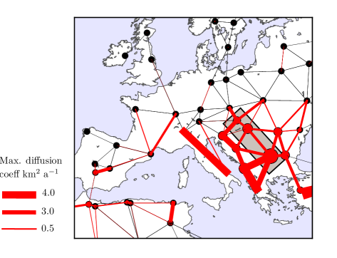
Unlike in many other models, the diffusion coefficient $D$ here is an emergent property, that varies in space and time, and that varies among all neighbors of each region. The diffusion coefficient varies between zero and 7 km² a^-1; Figure 17.5 shows the topology of the interregional connections in Europe and their maximum diffusion coefficients. Maximum diffusion is highest on the Balkan and within Italy (up to 4 km² a^-1), it is one order of magnitude lower for all of Northern Europe. This shows the importance of the Balkans as a central hub for the diffusion of Neolithic technology, people, and ideas; there seem to have been main routes for Neolithic diffusion across the central Balkan, along Adriatic coastlines, or, to a lesser extent, up the Rh^one valley.

The diffusion coefficient $D$ seems first and foremost to match the migration rate of populations of ultimately Anatolian/Near Eastern ancestry into and within Europe. On a continental scale this rate should have been higher in Southeastern Europe and possibly in Italy, equally along the Rhône. This is supported by recent archaeological and archaeogenetic data, at least for Southeastern and Central Europe  [18] [19]. Therefore, it is to be assumed that the proportion of non-indigenous populations should have been highest in these areas. Towards the north the spread of these immigrant Neolithic populations was halted until about 4000 BCE, after which farming spread further into the European north and northwest as well as to the British Isles. This stagnation pattern is visible from archaeological evidence [15] [35] and represented in model simulations [36]. Towards the continental west the evidence for a lesser proportion of allochtonous cultural traits in the archeological record of farming societies has continuously been interpreted as an increase in indigenous populations within these societies; therefore the rate of immigrants should have been lower. This has at least been suggested by archaeology [37]; recent genetic studies have shown, however, that the influx of a population of ultimately Balkanic/Anatolian origin seems also to have been strong at least in the Paris Basin and eastern France [38].

While the simulated Neolithic transition is reasonably well reflected on the continental scale, the model skill in representing the individual regional spatial expansions varies. For example, the particular geographic expansion of the LBK in Central Europe occurs too late and is too small in extent towards the Paris Basin. On the other hand, the timing of the arrival of the Neolithic in the Balkans, in southern Spain, or in northern Europe is well represented [36].

Figure 17.6: Time evolution of the diffusion coefficient for three selected regions of central Europe (Bulgaria, Serbia, Hungary; shown in black, red, and blue, respectively). For each of these three regions, the family of trajectories represents the region’s diffusion coefficients with respect to each of its adjacent regions. The shaded bars indicate the time interval of a regional transition to agropastoralism in the simulation (10–90% of $C$).

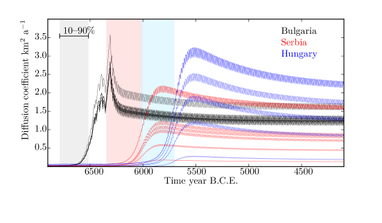
For three selected regions along the central Balkan diffusion main route (highlighted in Figure 17.5) we analysed the temporal evolution of their diffusion coefficients (Figure 17.6). A similar pattern is visible in all three regions and all diffusion coefficients: $D$ starts at zero, then rapidly rises to a marked peak and slowly decays asymptotically to an intermediate value. This behavior is a consequence of the local influence and its difference to adjacent regions. Initially the influence difference is zero, because all regions have similar technology and population. As soon as one region innovates (or receives via diffusion technology and population from one of its neighbors), population and technology increase, and so does the influence difference to all other neighbors. With an increase in influence and diffusion coefficient, demic and cultural diffusion to neighbors decrease the influence differences. Relative proportions among the diffusion coefficients of one region to all its neighbors are constant and attributed to the geographical setting.

The time evolution of the diffusion coefficient plotted in Figure 17.6 reflects the population statistics for advancing Neolithic technology: Early farming appears to be associated to a rapid increase in population, this on a supra-regional scale [39] [40]. At the regional level, the diffusion coefficient lags the onset of farming by several hundred years. This lag is also empirically reflected in the data set of the western LBK [41]. Any pioneering farming society seems to have followed more or less the same general population trajectory with a gradual increase over several centuries, followed by a sudden rise-and-decline. The causes for this general pattern are yet unclear, but may have to be sought more in social behavior patterns rather than purely economic or environmental determinants [42].

17.4 Conclusion

It has been long evident, that the Neolithic “Revolution” is not a single event, but heterogeneous in space and time. Statistical models for understanding the diffusion processes, however, have so far assumed that a physical model of Fickian diffusion can be applied to the pattern of the emergence of farming and pastoralism using constant diffusion coefficients. Relaxing this constraint, and reformulating the diffusivity as a function of influence differences between regions, demonstrates how diffusivity varies in space and time.

When results using this variable correlation coefficient ($D$) are compared to empirical archaeological data, they represent the dynamics on a continental scale and on the regional scale for many regions well, but not for all: The impetus of the Neolithic in Greece and the Balkans is well represented, also in southeastern Central Europe. The emergence and the expansion of the Central European LBK shows, however, a too early expansion in the model, whereas the stagnation following the initial expansion is again very well represented.

Divergence between the mathematical model and the empirical findings provided by archaeology is unsurprising and expected, because human societies behave in much more complex ways than are described in the highly aggregated and simplified model. Individuals may have chosen to act independent of the social and environmental context and against rational maximization of benefits. Rather than perfectly capturing each regional diffusion event, the mathematical model serves as a null hypothesis which is broadly consistent with the archaeologically reconstructed picture, and against which individual decisions can be assessed. In this respect, the simple model helps to disentangle in complex histories general forcing agents and individual choices.

References

[1]V. G. Childe, Dawn Of European Civilization, 1st ed. (Routledge [reprinted 2005], 1925), p. 256.

[2]N. Goring-Morris and A. Belfer-Cohen, Current Anthropology 52, (2011).

[3]G. Barker, The Agricultural Revolution in Prehistory: Why Did Foragers Become Farmers? (Oxford University Press, Oxford, United Kingdom, 2006), p. 616.

[4]W. F. Ruddiman, D. Q. Fuller, J. E. Kutzbach, P. C. Tzedakis, J. O. Kaplan, E. C. Ellis, S. J. Vavrus, C. N. Roberts, R. Fyfe, F. He, C. Lemmen, and J. Woodbridge, Reviews of Geophysics 54, 93 (2016).

[5]P. Bellwood, First Farmers: The Origins of Agricultural Societies, 1st ed. (Wiley-Blackwell, Malden, 2004), p. 384.

[6]E. M. Gallagher, S. J. Shennan, and M. G. Thomas, Proceedings of the National Academy of Sciences 112, 201511870 (2015).

[7]J. G. D. Clark, Proceedings of the Prehistoric Society 31, 57 (1965).

[8]M.-j. Gaillard, S. Sugita, F. Mazier, J. O. Kaplan, A.-K. Trondman, A. Broström, T. Hickler, E. Kjellström, P. Kuneš, C. Lemmen, J. Olofsson, B. Smith, and G. Strandberg, Climate of the Past Discussions 6, 307 (2010).

[9]H. J. Zahid, E. Robinson, and R. L. Kelly, Proceedings of the National Academy of Sciences 201517650 (2015).

[10]B. G. Purzycki, C. Apicella, Q. D. Atkinson, E. Cohen, R. A. McNamara, A. K. Willard, D. Xygalatas, A. Norenzayan, and J. Henrich, Nature 530, 327 (2016).

[11]J.-P. Bocquet-Appel, S. Naji, M. Vander Linden, and J. Kozlowski, Journal of Archaeological Science 39, 531 (2012).

[12]F. Silva, J. Steele, K. Gibbs, and P. Jordan, Radiocarbon 56, 723 (2014).

[13]K. Manning, S. S. Downey, S. Colledge, J. Conolly, B. Stopp, K. Dobney, and S. Shennan, Antiquity 87, 1046 (2013).

[14]A. Bogaard, Neolithic Farming in Central Europe : An Archaeobotanical Study of Crop Husbandry Practices (Routledge, 2004), p. 210.

[15]W. Schier, Praehistorische Zeitschrift 84, 15 (2009).

[16]F.-X. Ricaut, Advances in Anthropology 02, 14 (2012).

[17]W. Haak, I. Lazaridis, N. Patterson, N. Rohland, S. Mallick, B. Llamas, G. Brandt, S. Nordenfelt, E. Harney, K. Stewardson, Q. Fu, A. Mittnik, E. Bánffy, C. Economou, M. Francken, S. Friederich, R. G. Pena, F. Hallgren, V. Khartanovich, A. Khokhlov, M. Kunst, P. Kuznetsov, H. Meller, O. Mochalov, V. Moiseyev, N. Nicklisch, S. L. Pichler, R. Risch, M. a. Rojo Guerra, C. Roth, A. Szécsényi-Nagy, J. Wahl, M. Meyer, J. Krause, D. Brown, D. Anthony, A. Cooper, K. W. Alt, and D. Reich, Nature 522, 207 (2015).

[18]G. Brandt, A. Szécsényi-Nagy, C. Roth, K. W. Alt, and W. Haak, Journal of Human Evolution 79, 73 (2015).

[19]Z. Hofmanová, S. Kreutzer, G. Hellenthal, C. Sell, Y. Diekmann, D. Díez del Molino, L. van Dorp, S. López, A. Kousathanas, V. Link, K. Kirsanow, L. M. Cassidy, R. Martiniano, M. Strobel, A. Scheu, K. Kotsakis, P. Halstead, S. Triantaphyllou, N. Kyparissi-Apostolika, D.-C. Urem-Kotsou, C. Ziota, F. Adaktylou, S. Gopalan, D. M. Bobo, L. Winkelbach, J. Blöcher, M. Unterländer, C. Leuenberger, Ç. Çilingiroğlu, B. Horejs, F. Gerritsen, S. Shennan, D. G. Bradley, M. Currat, K. Veeramah, D. Wegmann, M. G. Thomas, C. Papageorgopoulou, and J. Burger, Proceedings of the National Academy of Sciences of the United States of America (2016).

[20]A. Ammerman and L. Cavalli Sforza, The Neolithic Transition and the Population Genetics of Europe. (Princeton University, Princeton, NJ, 1984).

[21]J. Fort, Proceedings of the National Academy of Sciences of the United States of America 109, 18669 (2012).

[22]C. Lemmen, D. Gronenborn, and K. W. Wirtz, Journal of Archaeological Science 38, 3459 (2011).

[23]C. Lemmen, Archaeology, Ethnology and Anthropology of Eurasia 41, 48 (2013).

[24]C. Lemmen and A. Khan, in Climates, Landscapes, and Civilizations, edited by L. Giosan, D. Q. Fuller, K. Nicoll, R. K. Flad, and P. D. Clift (American Geophysical Union, Washington, 2012), pp. 107–114.

[25]K. W. Wirtz and C. Lemmen, Climatic Change 59, 333 (2003).

[26]B. Arıkan, Journal of Archaeological Science 43, 38 (2014).

[27]E. Boserup, Population and Technological Change (University of Chicago Press, 1981), p. 255.

[28]J. A. J. Metz, R. M. Nisbet, and S. A. H. Geritz, Trends in Ecology and Evolution 7, 198 (1992).

[29]R. A. Fisher, The Genetical Theory of Natural Selection (Dover, Oxford, 1930).

[30]K. W. Wirtz and B. Eckhardt, Ecological Modelling 92, 33 (1996).

[31]K. W. Wirtz, Modellierung von Anpassungsvorgängen in der belebten Natur (Universität Kassel, 1996), p. 216.

[32]C. Lemmen, Documenta Praehistorica XLII, 93 (2015).

[33]K. Davison, P. M. Dolukhanov, G. R. Sarson, and A. Shukurov, Journal of Archaeological Science 33, 641 (2006).

[34]R. Pinhasi, J. Fort, and A. J. Ammerman, Public Library of Science Biology 3, (2005).

[35]A. W. R. Whittle, F. M. A. Healy, and A. Bayliss, Gathering Time: Dating the Early Neolithic Enclosures of Southern Britain and Ireland (Oxbow Books, 2011).

[36]C. Lemmen and K. W. Wirtz, Journal of Archaeological Science 51, 65 (2014).

[37]C. Jeunesse and S. Van Willigen, in The Spread of the Neolithic to Central Europe (Mainz, Germany, 2010), pp. 569–605.

[38]M. Rivollat, H. Réveillas, F. Mendisco, M.-H. Pemonge, P. Justeau, C. Couture, P. Lefranc, C. Féliu, and M.-F. Deguilloux, American Journal of Physical Anthropology 161, 522 (2016).

[39]J.-P. Bocquet-Appel, Science 333, 560 (2011).

[40]S. J. Shennan, S. S. Downey, A. Timpson, K. Edinborough, S. Colledge, T. Kerig, K. Manning, and M. G. Thomas, Nature Communications 4, 1 (2013).

[41]D. Gronenborn, H.-C. Strien, S. Dietrich, and F. Sirocko, Journal of Archaeological Science 51, 73 (2014).

[42]D. Gronenborn, H.-C. Strien, and C. Lemmen, Quaternary International, in press (2017).