The GOODS-N Jansky VLA 10 GHz Pilot Survey: Sizes of Star-Forming $\mu$Jy Radio Sources

Abstract

Our sensitive ($\sigma_{\mathrm{n}}\approx 572\mathrm{\,nJy\,beam}^{-1}$), high-resolution (FWHM $\theta_{1/2}=0\,\farcs 22\approx 2\mathrm{\,kpc~{}at~{}}z\gtrsim 1$) 10 GHz image covering a single Karl G. Jansky Very Large Array (VLA) primary beam (FWHM $\Theta_{1/2}\approx 4\farcm 25$) in the GOODS-N field contains 32 sources with $S_{\mathrm{p}}\gtrsim 2\,\mu\mathrm{Jy~{}beam}^{-1}$ and optical and/or near-infrared (OIR) counterparts. Most are about as large as the star-forming regions that power them. Their median FWHM major axis is $\langle\theta_{\mathrm{M}}\rangle=167\pm 32\mathrm{\,mas}\approx 1.2\pm 0.28\mathrm{\,kpc}$ with rms scatter $\approx 91\mathrm{\,mas}\approx 0.79\mathrm{\,kpc}$. In units of the effective radius $r_{\rm e}$ that encloses half their flux, these radio sizes are $\langle r_{\rm e}\rangle\approx 69\pm 13\mathrm{\,mas}\approx 509\pm 114\mathrm{\,pc}$ and have rms scatter $\approx 38\mathrm{\,mas}\approx 324\mathrm{\,pc}$. These sizes are smaller than those measured at lower radio frequencies, but agree with dust emission sizes measured at mm/sub-mm wavelengths and extinction-corrected H$\alpha$ sizes. We made a low-resolution ($\theta_{1/2}=1\farcs 0$) image with $\approx 10\times$ better brightness sensitivity to detect extended sources and measure matched-resolution spectral indices $\alpha_{\rm 1.4\,GHz}^{\rm 10\,GHz}$. It contains 6 new sources with $S_{\mathrm{p}}\gtrsim 3.9\,\mu\mathrm{Jy~{}beam}^{-1}$ and OIR counterparts. The median redshift of all 38 sources is $\langle z\rangle=1.24\pm 0.15$. The 19 sources with 1.4 GHz counterparts have median spectral index $\langle\alpha_{\rm 1.4\,GHz}^{\rm 10\,GHz}\rangle=-0.74\pm 0.10$ with rms scatter $\approx 0.35$. Including upper limits on $\alpha$ for sources not detected at 1.4 GHz flattens the median to $\langle\alpha_{\rm 1.4\,GHz}^{\rm 10\,GHz}\rangle\gtrsim-0.61$, suggesting that the $\mu$Jy radio sources at higher redshifts, and hence selected at higher rest-frame frequencies, may have flatter spectra. If the non-thermal spectral index is $\alpha_{\rm NT}\approx-0.85$, the median thermal fraction of sources selected at median rest-frame frequency $\approx 20$ GHz is $\gtrsim$48%.

1. Introduction

Most radio surveys aimed at measuring the star-formation history of the universe have been made at 1.4 or 3 GHz Schinnerer et al., 2007; Morrison et al., 2010, (e.g.,; Smolčić et al. 2016, in press), so they are more sensitive to steep-spectrum synchrotron radiation than flat-spectrum free-free emission. Low frequencies were favored because telescope primary beam areas decrease with frequency ($\Omega_{\rm PB}\propto\nu^{-2}$) and the steep decimetric spectra of star-forming galaxies $\langle\alpha\rangle\approx-0.7$, where $S_{\nu}\propto\nu^{\alpha}$ (Condon, 1992), often cause “survey speed” to decline sharply with frequency: $SS\propto\nu^{-3.4}$ if system temperature, bandwidth, etc. are fixed. For a detailed quantitative discussion, see Condon (2015). Although more difficult to detect, higher-frequency radio emission from galaxies provides independent information on galaxy energetics and the star-formation process. Constructing the star-formation history of the universe requires converting the synchrotron luminosities measured by low frequency surveys to star-formation rates via the tight, but empirical and local, far-infrared/radio correlation (de Jong et al., 1985; Helou et al., 1985; Yun et al., 2001). Surveys at observing frequencies $\gtrsim$10 GHz measure flux densities closer to the rest-frame frequencies $\nu\gtrsim 30\mathrm{\,GHz}$, where the total radio emission is dominated by the free-free radiation that is more directly proportional to the rate of massive star formation (e.g., Mezger & Henderson, 1967; Klein & Graeve, 1986; Turner & Ho, 1983, 1985; Kobulnicky & Johnson, 1999; Murphy et al., 2012b; Nikolic & Bolton, 2012; Murphy et al., 2015b), are still unbiased by dust emission or absorption, and yield higher angular resolution for a given array size.

Using the original VLA, Richards et al. (1998, 1999) reached $\sigma_{\mathrm{n}}=8.5\,\mu\mathrm{Jy~{}beam}^{-1}$ at 8.5 GHz in the Hubble Deep Field-North (HDF-N, Williams et al., 1996). The significantly increased bandwidth of the upgraded VLA now allows more sensitive surveys in a reasonable amount of observing time. Furthermore, the VLA will remain the only radio interferometer able to conduct such high-frequency radio continuum surveys until the SKA1-MID comes online equipped with the Band-5a/b ($5-9.25$ GHz/$9-16.7$ GHz) receivers perhaps in $\gtrsim$2025 (e.g., Murphy et al., 2015a).

In this paper, we present initial results on a flux-limited sample of galaxies from pilot observations aimed at mapping the entire Great Observatories Origins Deep Survey-North (GOODS-N; Dickinson et al., 2003; Giavalisco et al., 2004) field at 10 GHz. The GOODS-N field at J2000 $\alpha=12^{\mathrm{h}}36^{\mathrm{m}}55^{\mathrm{s}},\delta=+62\arcdeg 14\arcmin 15\arcsec$ covers $\approx 160$ arcmin² centered on the HDF-N and is unrivaled in terms of its ancillary data. These include extremely deep Chandra, Hubble Space Telescope (HST), Spitzer, and Herschel observations, deep $UBVRIJHK$ ground-based imaging, $\sim$3500 spectroscopic redshifts from 8–10 m telescopes, and some of the deepest 1.4 GHz observations ever made (Morrison et al., 2010). Our new VLA X-band ($8-12$ GHz; reference frequency 10 GHz) pilot image has $\approx 15\times$ better point-source sensitivity than the Richards et al. (1998) image. Its $\theta_{1/2}\approx 0\,\farcs 22$ angular resolution is well matched to the resolution of HST/ACS optical and HST/WFC3-IR (continuum + H$\alpha$ imaging) data from GOODS and the Cosmic Assembly Near-Infrared Deep Extragalactic Legacy Survey (CANDELS; Grogin et al., 2011; Koekemoer et al., 2011), and delivers a physical resolution of $\lesssim 1.9\mathrm{\,kpc}$ at any redshift. Finally, the radio data provide an extinction-free view of the morphologies of dusty starburst galaxies which dominate the cosmic star-formation activity between $1\lesssim z\lesssim 3$ (e.g., Murphy et al., 2011a; Magnelli et al., 2013). In this redshift range, 10 GHz observations sample $20\lesssim\nu\lesssim 40\mathrm{\,GHz}$ in the source frame, where galaxy emission is expected to be dominated by free-free radiation (e.g., Murphy, 2009) and thus provide accurate star-formation rates for comparison with other diagnostics available from the GOODS ancillary data (e.g., FUV continuum, H$\alpha$, [Oiii]5007 Å).

In this paper we highlight our findings on the typical 10 GHz source characteristics based on these new, extremely deep VLA data. The paper is organized as follows: In §2 we describe the data as well as the analysis procedures used in the present study. In §3 we present our results and discuss their implications. Our main conclusions are then summarized in §4. All calculations are made assuming a Hubble constant $H_{0}=71\mathrm{~{}km~{}s}^{-1}\mathrm{~{}Mpc}^{-1}$ and a flat $\Lambda$CDM cosmology with $\Omega_{\rm M}=0.27$ and $\Omega_{\Lambda}=0.73$.

2. Data and Analysis

In this section we describe our observations and imaging procedure. We additionally describe in detail our source-finding and optical/NIR (OIR) cross-matching procedure used to create a highly reliable final sample of sources.

2.1. Observations

We observed a single pointing centered on J2000 $\alpha=12^{\mathrm{h}}36^{\mathrm{m}}51\fs 26,\delta=+62\arcdeg 13\arcmin 37\farcs 4$ over the $8-12$ GHz X-band frequency range with the A- and C-configurations as part of the project VLA/14B-037. We chose this pointing center to maximize the overlap of known sources in GOODS-N detected at other frequencies, specifically the $31-39$ GHz continuum detections from VLA project VLA/13A-398 (PI: Riechers) that searched for redshifted 115 GHz CO $J=1\rightarrow 0$. These continuum detection results (J. Hodge et al., in preparation) remain unpublished and are thus not included in the present analysis. We utilized two pairs of the 3-bit samplers of the VLA, each with 2 GHz bandwidth and dual polarization (R and L). For each sampler pair the Wideband Interferometric Digital ARchitecture (WIDAR) correlator delivered 16 sub-bands, each 128 MHz wide with 2 MHz spectral channels and full polarization products (RR, LL, RL, LR).

The on-source integration times in the A and C configurations were roughly 23 and 1.5 hr, respectively. The A-configuration observations were carried out over seven separate runs during 2015 June, and the C-configuration observations were made during a single run in 2014 December. The source 3C 286 was used as the flux density scale and bandpass calibrator, while J1302+5748 was used as the complex gain and telescope pointing calibrator. Full polarization information was additionally obtained, using 3C 286 to calibrate the polarization position angle and J1407+2827 as a instrumental polarization (leakage) calibrator. However, the polarization results will be deferred to a future paper. To reduce these data, we used the Common Astronomy Software Applications (CASA; McMullin et al., 2007) package and followed standard calibration and editing procedures, including the utilization of the VLA calibration pipeline.

2.2. Imaging

The calibrated A- and C-configuration measurement sets were imaged together using the task tclean in CASA version 4.6. The inclusion of the C-configuration data helps to fill in the hole in the $(u,v)$-plane left by the A-configuration data alone that, if not accounted for, will reduce the integrated flux densities of extended sources. The mode of tclean was set to multifrequency synthesis (mfs; Conway et al., 1990; Sault & Wieringa, 1994). After significant experimentation, we chose to use Briggs weighting with robust=0.5 and set the parameter nterms=2. nterms is the number of Taylor terms to model the frequency dependence of the sky emission. The value of 2 allows the mfs cleaning procedure to fit sources with different spectral indices in addition to the sources’ intensities. The use of Briggs weighting is necessary to suppress the broad pedestal of the naturally-weighted dirty beam of the VLA A configuration, and thus helps to suppress sidelobes. To deconvolve extended low-intensity emission, we took advantage of the multiscale clean option (Cornwell, 2008; Rau & Cornwell, 2011) in CASA, searching for structures with scales up to $\approx 16\times$ the FWHM of the synthesized beam (i.e., about $\approx 2\times$ larger than the FWHM of the synthesized beam in the C configuration). We additionally invoked the W-projection algorithm (Cornwell et al., 2005, 2008) using 16 W-planes to take the non-coplanar nature of the array into account.

To improve the quality of the dirty beam by both making its shape more nearly Gaussian and further suppressing sidelobe structure, we applied a taper for baselines longer than $\sim 10^{6}\lambda$. This taper was found to produce the best combination of brightness-temperature and point-source sensitivity. The main lobe of the dirty beam was nearly a circular Gaussian (major and minor FWHMs $\theta_{\mathrm{maj}}=0\,\farcs 223\times\theta_{\mathrm{min}}=0\,\farcs 206$); thus, for simplicity, we restored the final image with a circular Gaussian with FWHM $\theta_{1/2}=0\,\farcs 22$. The final high-resolution image used in this analysis is a $10\arcmin$ on a side square and within 5% of the primary beam response has an rms noise $\sigma_{\mathrm{n}}\approx 572\mathrm{\,nJy\,beam}^{-1}\approx 139\mathrm{\,mK}$ at the image center. For a primary beam FWHM at 10 GHz of $\Theta_{1/2}\approx 4\farcm 25$, the image is approximately $2.35\times\Theta_{1/2}$ on a side. For sources with typical spectral indices $\alpha\approx-0.7$, the point-source sensitivity at the center of the 10 GHz image is $\approx 2\times$ more sensitive than that of the Morrison et al. (2010) 1.4 GHz image, which has $\theta_{1/2}=1\,\farcs 7$ resolution and rms noise $\sigma_{\mathrm{n}}\sim 4\,\mu\mathrm{Jy\,beam}^{-1}$.

We additionally made $(u,v)$-tapered images having 1″and 2″ synthesized beams to increase the brightness-temperature sensitivity of our observations and investigate if our high-resolution image missed significant numbers of extended sources. The tapered 1″and 2″ images have an rms noises $\sigma_{\mathrm{n}}\approx 1.1\,\mu\mathrm{Jy\,beam}^{-1}$ and $\sigma_{\mathrm{n}}\approx 1.5\,\mu\mathrm{Jy\,beam}^{-1}$, respectively, or roughly $2\times$ and $3\times$ higher than our full-resolution image. However, the corresponding brightness temperature rms values of the 1″and 2″ tapered images are $\sigma_{\mathrm{n}}\approx 13\mathrm{\,mK}$ and $\sigma_{\mathrm{n}}\approx 4.7\mathrm{\,mK}$, or $\approx 10\times$ and $\approx 30\times$ lower than our full-resolution image, respectively.

Figure 1.— A model radio spectrum of a $z=1$ galaxy forming stars at a rate of $\psi\approx 25\,M_{\odot}\,$yr^-1. Synchrotron, free-free, and thermal dust emission components are identified, along with the $J=2\rightarrow 1$ and $J=1\rightarrow 0$ emission lines of CO. The grayed region identifies the rest-frame bandpass of our 10 GHz observations for such a source, illustrating that at $z\gtrsim 1$ these data should become sensitive to free-free emission, and hence current star formation activity in high-redshift galaxies.

2.2.1 Sensitivity of Deep Radio Imaging to Star Forming Galaxies at High-Redshift

Coupling the relation between total infrared (IR; $8-1000\mu$m) luminosity and star formation rate in Murphy et al. (2012b, Equation 15), which assumes a Kroupa (Kroupa, 2001) initial mass function (IMF), with the locally measured IR-radio correlation (i.e., $q_{\rm IR}=2.64$; Bell, 2003), the star formation rate of a galaxy is related to its 1.4 GHz spectral luminosity by

$$\psi(M_{\odot}\mathrm{\,yr}^{-1})\approx 5.16\times 10^{-29}\Biggl{(}\frac{L_{\mathrm{1.4\,GHz}}}{\mathrm{erg\,s^{-1}\,Hz}^{-1}}\Biggr{)}~{}.$$ (1)

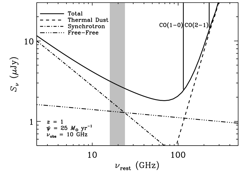
At $z=1$, a $5\sigma_{\mathrm{n}}=2.86\,\mu\mathrm{Jy\,beam}^{-1}$ 10 GHz point source with a spectral index $\alpha=-0.7$ has a spectral luminosity $L_{\mathrm{1.4\,GHz}}\approx 4.85\times 10^{29}\mathrm{\,erg\,s^{-1}\,Hz}^{-1}$, so Equation 1 gives a star-formation rate $\psi\approx 25\,M_{\odot}\,\mathrm{yr}^{-1}$.

A model radio-to-far–infrared spectrum of such a galaxy is illustrated in Figure 1, indicating how these 10 GHz observations are highly sensitive to the amount of free-free emission at $z\gtrsim 1$, and hence current star formation. Furthermore, at the low radio flux densities achieved by our deep 10 GHz imaging, the fraction of active galactic nuclei (AGN) detected relative to star-forming galaxies is extremely low (e.g., Condon, 1984; Wilman et al., 2008). In Figure 4 of Wilman et al. (2008), the AGN fraction at several frequencies are shown including 1.4, 4.8, and 18 GHz, where the lowest AGN fraction is indeed found at the highest frequency of 18 GHz, being $\lesssim 10$%. Consequently, by being sensitive to free-free emission from galaxies forming stars at a rate of $\psi\gtrsim 25\,M_{\odot}\,\mathrm{yr}^{-1}$ at $z\sim 1$, our 10 GHz data are sensitive to galaxies that contribute to roughly half of the cosmic star formation rate density at these epochs (e.g., Murphy et al., 2011a; Magnelli et al., 2013). Furthermore, given this star formation rate threshold, our data reach a mass-limit where the $z\sim 1$ cosmic star formation rate density peaks, and hence down to the most representative star forming sources at this epoch (Karim et al., 2011).

2.3. Source Finding and Photometry

We used the PyBDSM (Mohan & Rafferty, 2015) source detection package to locate and measure the integrated flux densities of the radio sources in each of our images. To do this, PyBDSM identifies “islands” of contiguous pixels above a detection threshold and fits each island with Gaussians. We ran PyBDSM over the entire image using the standard default setting, except that we lowered the pixel threshold for keeping fitted sources from 5 to $3.5\sigma_{\mathrm{n}}$. We adopted a minimum threshold of $3.5\sigma_{\mathrm{n}}$ as we consider such sources having optical identifications potentially significant. A primary beam correction was then applied to the reported peak brightnesses and integrated flux densities (along with their errors) using the frequency-dependent primary beam correction at 10 GHz given in EVLA Memo# 195 (Perley 2016). For this paper, we kept sources out to a radius of $\approx 3\,\farcm 9$ from the phase center, where the sky response drops to $\approx 5$% of the on-axis value. For reference, the HWHM of the primary beam at 10 GHz is $\approx 2\farcm 125$. A total of 1412 and 114 sources were “detected” (see §2.3.2) above a threshold of 3.5 and $5\sigma_{\mathrm{n}}$, respectively. To assess the reliability of detections as faint as $3.5\sigma_{\mathrm{n}}$, we used existing deep HST and Spitzer data to identify OIR counterparts.

In Table 2.3 we list the deconvolved source parameters from PyBDSM for detections from the full-resolution image that are confirmed by having OIR counterparts (see §2.3.1). Sources are split by their 10 GHz detection confidence, being either at a significance of $S_{\mathrm{P}}/\sigma_{\mathrm{n}}\geq 5$ or $3.5\leq S_{\rm P}/\sigma_{\mathrm{n}}<5$. It is worth emphasizing that images from the full survey, which will include multiple pointings per source, will be able to confirm any questionable sources without OIR counterparts detected in these single-pointing pilot observations. Listed parameters include the source positions, peak brightnesses ($S_{\rm P}$), integrated flux densities ($S_{\rm I}$), best estimates for the total flux densities ($S_{\rm*}$) and deconvolved FWHM source sizes ($\theta_{\rm M}\times\theta_{\rm m}$). Deconvolved source sizes were calculated such that

$$\theta=\sqrt{\phi^{2}-\theta_{1/2}^{2}}~{},$$ (2)

where $\phi$ is the FWHM of the fitted major or minor axis. The uncertainties in the fitted parameters include the effects of correlated noise in synthesis images (Condon, 1997). Uncertainties on the deconvovled source sizes were calculated as follows

$$\left(\frac{\sigma_{\theta}}{\sigma_{\phi}}\right)=\left[1-\left(\frac{\theta_{1/2}}{\phi}\right)^{2}\right]^{-1/2}~{}.$$ (3)

For a few sources, PyBDSM fit multiple Gaussian components, typically including a very narrow component at the peak of the source. One instance of this is for the known FR I radio galaxy at $z=1.013$ (Richards et al., 1998), where we are able to resolve some of its jet structure. Because we are interested in measuring the extent of star-forming galaxy disks, we used imfit in CASA to fit single Gaussians for these cases and report the corresponding deconvolved source parameters.

Individual sources are considered to be confidently resolved if $\phi_{\rm M}-\theta_{1/2}\geq 2\sigma_{\phi_{\rm M}}$, and are identified in Tables 2.3 and The GOODS-N Jansky VLA 10 GHz Pilot Survey: Sizes of Star-Forming $\mu$Jy Radio Sources. For instances where PyBDSM reported unphysical fitted sizes, being equal to or smaller than the synthesized beam, a size of 0 in listed in Tables 2.3 and The GOODS-N Jansky VLA 10 GHz Pilot Survey: Sizes of Star-Forming $\mu$Jy Radio Sources where the associated uncertainty corresponds to the 1$\sigma$ upper limit of the deconvolved source size. For sources whose major axes are resolved, the integrated flux densities from the source fitting are taken as the best estimate for the sources total flux density ($S_{*}$). For sources whose fitted major axes are less than 2$\sigma_{\phi_{\rm M}}$ larger than the synthesized beam, we instead take their total flux density to be the geometric mean of the peak brightness and integrated flux densities reported by PyBDSM (Condon, 1997).

In Table The GOODS-N Jansky VLA 10 GHz Pilot Survey: Sizes of Star-Forming $\mu$Jy Radio Sources, we similarly list the deconvolved source parameters and photometry from the 1″ $(u,v)$-tapered image, or from the 2″ image in the three cases where the total flux density in the 2″ image is $>3\sigma$ larger than in the 1″ image. The flux densities recovered in the 2″ tapered image for these three sources are larger by factors of $\approx 1.1$, 2.9, and 1.2 in order of appearance in Table The GOODS-N Jansky VLA 10 GHz Pilot Survey: Sizes of Star-Forming $\mu$Jy Radio Sources.

Table 1Full Resolution 10 GHz Source Characteristics

$S_{\rm P}/\sigma_{\rm n}\geq 5$

$12~{}36~{}34.211$ $+62~{}14~{}32.95$ 0.5184 1 31 19.52 $7.72\pm 1.24$ $8.71\pm 2.09$ $8.20\pm 1.24$ $148\pm 86\times 0\pm 118$
^d$12~{}36~{}34.514$ $+62~{}12~{}41.08$ 1.2234 1 139 21.11 $9.02\pm 1.23$ $27.90\pm 4.87$ $27.90\pm 4.87$^e $354\pm 69\times 283\pm 59$
$12~{}36~{}42.091$ $+62~{}13~{}31.43$ 2.018 1 16 23.76 $37.81\pm 0.70$ $36.80\pm 1.22$ $37.30\pm 0.70$ $42\pm 23\times 0\pm 41$
$12~{}36~{}42.214$ $+62~{}15~{}45.51$ 0.8575 1 173 20.02 $27.78\pm 1.47$ $32.87\pm 2.42$ $32.87\pm 2.42$^e $144\pm 28\times 0\pm 69$
$12~{}36~{}44.110$ $+62~{}12~{}44.81$ 1.676 2 49 21.85 $3.97\pm 0.74$ $4.46\pm 1.25$ $4.21\pm 0.74$ $171\pm 100\times 0\pm 120$
^d$12~{}36~{}44.386$ $+62~{}11~{}33.14$ 1.0128 1 30 19.46 $279.25\pm 2.14$ $340.57\pm 4.25$ $340.57\pm 4.25$^e $139\pm 4\times 56\pm 7$
$12~{}36~{}46.063$ $+62~{}14~{}48.70$ 2.003 1 155 23.71 $6.95\pm 0.82$ $10.65\pm 1.25$ $10.65\pm 1.25$^e $214\pm 57\times 101\pm 62$
$12~{}36~{}46.332$ $+62~{}14~{}04.69$ 0.9605 1 82 20.11 $92.69\pm 0.64$ $91.06\pm 1.12$ $91.06\pm 1.12$^e $53\pm 7\times 0\pm 25$
$12~{}36~{}48.076$ $+62~{}13~{}09.01$ 0.4745 1 35 19.59 $4.22\pm 0.64$ $4.38\pm 1.09$ $4.30\pm 0.64$ $80\pm 108\times 0\pm 121$
$12~{}36~{}48.330$ $+62~{}14~{}16.57$ 2.002 1 149 22.55 $3.20\pm 0.63$ $3.15\pm 1.13$ $3.17\pm 0.63$ $146\pm 114\times 0\pm 118$
$12~{}36~{}52.884$ $+62~{}14~{}44.07$ 0.3208 1 18 18.22 $114.69\pm 0.72$ $113.24\pm 1.25$ $113.96\pm 0.72$ $25\pm 13\times 0\pm 24$
$12~{}36~{}53.367$ $+62~{}11~{}39.58$ 1.268 1 45 21.47 $5.43\pm 1.03$ $20.82\pm 1.28$ $20.82\pm 1.28$^e $553\pm 140\times 220\pm 73$
$12~{}36~{}55.449$ $+62~{}13~{}11.24$ 0.9544 1 11 20.63 $20.11\pm 0.64$ $20.53\pm 1.11$ $20.32\pm 0.64$ $54\pm 31\times 0\pm 55$
$12~{}36~{}56.914$ $+62~{}13~{}01.64$ 1.2409 1 21 21.16 $8.69\pm 0.66$ $8.12\pm 1.17$ $8.40\pm 0.66$ $24\pm 160\times 0\pm 82$
$12~{}36~{}58.843$ $+62~{}14~{}34.92$ 0.6766 1 34 19.75 $4.71\pm 0.77$ $4.86\pm 1.32$ $4.78\pm 0.77$ $110\pm 98\times 0\pm 119$
$12~{}37~{}04.873$ $+62~{}16~{}01.55$ 1.170 1 16 23.20 $12.83\pm 2.24$ $13.02\pm 3.93$ $12.92\pm 2.24$ $145\pm 99\times 0\pm 113$
$12~{}37~{}11.251$ $+62~{}13~{}30.87$ 1.9958 1 11 22.40 $7.48\pm 1.35$ $8.15\pm 2.34$ $7.81\pm 1.35$ $181\pm 100\times 0\pm 113$
$12~{}37~{}11.984$ $+62~{}13~{}25.69$ 1.992 1 92 23.26 $7.30\pm 1.41$ $7.03\pm 2.56$ $7.16\pm 1.41$ $152\pm 113\times 0\pm 113$
$12~{}37~{}16.376$ $+62~{}15~{}12.35$ 0.5577 1 60 19.15 $87.07\pm 4.03$ $95.58\pm 6.78$ $91.22\pm 4.03$ $96\pm 29\times 23\pm 94$

$3.5\leq S_{\rm P}/\sigma_{\rm n}<5$

$12~{}36~{}19.565$ $+62~{}13~{}42.93$ 1.699 3 159 25.43 $31.16\pm 6.76$ $31.68\pm 11.85$ $31.42\pm 6.76$ $141\pm 124\times 0\pm 128$
$12~{}36~{}27.872$ $+62~{}14~{}49.08$ 0.6802 1 50 19.96 $12.78\pm 2.65$ $25.68\pm 3.78$ $18.12\pm 2.65$ $318\pm 112\times 122\pm 93$
$12~{}36~{}35.592$ $+62~{}14~{}24.04$ 2.0150 1 64 21.45 $4.90\pm 1.12$ $12.32\pm 1.51$ $7.77\pm 1.12$ $377\pm 131\times 171\pm 91$
$12~{}36~{}40.306$ $+62~{}13~{}31.14$ 0.484 1 66 21.24 $3.39\pm 0.72$ $3.88\pm 1.26$ $3.63\pm 0.72$ $238\pm 126\times 0\pm 112$
$12~{}36~{}41.604$ $+62~{}13~{}49.41$ 3.244 3 62 24.37 $3.20\pm 0.76$ $5.01\pm 1.16$ $4.00\pm 0.76$ $246\pm 121\times 65\pm 166$
$12~{}36~{}42.128$ $+62~{}13~{}48.34$ 0.817 3 81 25.32 $3.25\pm 0.71$ $3.41\pm 1.22$ $3.33\pm 0.71$ $119\pm 127\times 0\pm 138$
$12~{}36~{}46.736$ $+62~{}14~{}45.84$ 2.004 1 93 22.47 $3.45\pm 0.75$ $3.58\pm 1.29$ $3.51\pm 0.75$ $87\pm 148\times 0\pm 146$
$12~{}36~{}48.524$ $+62~{}14~{}36.91$ 1.365 3 88 26.68 $2.93\pm 0.69$ $2.95\pm 1.21$ $2.94\pm 0.69$ $126\pm 138\times 0\pm 138$
$12~{}36~{}49.688$ $+62~{}13~{}13.01$ 0.4745 1 179 20.61 $2.44\pm 0.66$ $3.32\pm 1.03$ $2.84\pm 0.66$ $173\pm 131\times 85\pm 164$
$12~{}36~{}57.375$ $+62~{}14~{}07.86$ 1.460 1 73 22.03 $2.95\pm 0.65$ $3.21\pm 1.14$ $3.07\pm 0.65$ $199\pm 125\times 0\pm 120$
$12~{}36~{}59.614$ $+62~{}11~{}53.36$ 1.0205 1 55 21.76 $4.25\pm 1.11$ $6.00\pm 1.75$ $5.05\pm 1.11$ $237\pm 137\times 0\pm 150$
$12~{}37~{}02.539$ $+62~{}13~{}02.32$ 2.650 4 145 25.63 $4.14\pm 0.83$ $6.84\pm 1.26$ $5.32\pm 0.83$ $292\pm 112\times 0\pm 131$
$12~{}37~{}08.748$ $+62~{}12~{}57.83$ 2.268 1 107 23.12 $5.89\pm 1.22$ $7.04\pm 2.01$ $6.44\pm 1.22$ $162\pm 107\times 0\pm 137$

2.3.1 Optical Identification

We identified our radio sources with their OIR counterparts in Momcheva et al. (2016) by position coincidence using the criteria presented in the Appendix of Condon et al. (1975). The radio position accuracy is noise limited, so the one-dimensional radio position errors parallel to the fitted FHWM major axis $\phi_{\mathrm{M}}$ and minor axis $\phi_{\mathrm{m}}$ are Gaussian distributed with rms

$$\sigma_{\mathrm{M}}\approx\frac{\phi_{\mathrm{M}}}{\sqrt{8\ln 2}}\biggl{(}\frac{\sigma_{\mathrm{P}}}{S_{\mathrm{P}}}\biggr{)}\mathrm{\quad and\quad}\sigma_{\mathrm{m}}\approx\frac{\phi_{\mathrm{m}}}{\sqrt{8\ln 2}}\biggl{(}\frac{\sigma_{\mathrm{P}}}{S_{\mathrm{P}}}\biggr{)},$$ (4)

respectively, where ($S_{\mathrm{P}}/\sigma_{\mathrm{P}}\approx S_{\mathrm{P}}/\sigma_{\mathrm{n}}$) is the fitted peak signal-to-noise ratio ($SNR$). Even $SNR=5$ point sources have very small $\sigma_{\mathrm{M}}\approx\sigma_{\mathrm{m}}\approx 0\,\farcs 019$. Nearly all of the OIR identifications have very high $SNR$, so their rms uncertainties $\sigma_{\mathrm{OIR}}$ are dominated by systematic differences between the OIR and radio reference frames. We made preliminary identifications and found systematic OIR minus radio offsets $\Delta\alpha=+3\,$mas and $\Delta\delta=+30\,$mas. After these offsets were removed, the remaining OIR errors have zero mean and rms $\sigma_{\mathrm{OIR}}\approx 0\,\farcs 025$.

If the radio and OIR sources coincide exactly on the sky, their measured radio-optical offsets $r$ should have a Rayleigh distribution

$$P(r)=\frac{r}{\sigma^{2}}\exp\biggl{(}-\frac{r^{2}}{2\sigma^{2}}\biggr{)}$$ (5)

with

$$\sigma\approx\sqrt{\left(\frac{\phi_{\rm M}}{\sqrt{8\ln{2}}}\frac{\sigma_{\mathrm{n}}}{S_{\mathrm{P}}}\right)^{2}+\sigma_{\rm OIR}^{2}}~{}.$$ (6)

The probability distribution of the angular distance $r$ from a radio source to the nearest unrelated optical object is

$$P(r)=2\pi\rho r\exp(-\pi\rho r^{2})~{},$$ (7)

where $\rho$ is the sky density of optical identification candidates. The mean angular distance to the nearest unrelated optical object is

$$\langle r\rangle=\frac{1}{2\sqrt{\rho}}~{}.$$ (8)

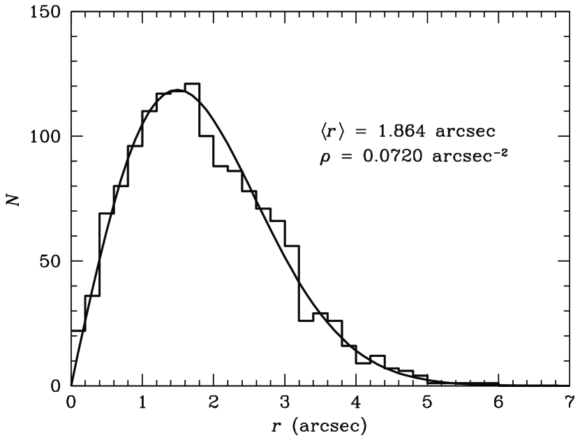
Figure 2 shows the distribution of angular distances $r$ to the OIR sources nearest to a large sample of random positions in our fields (histogram) and the best-fit Rayleigh distribution, which implies $\rho\approx 0.0720\mathrm{~{}arcsec}^{-2}$.

Figure 2.— This histogram showing the offsets $r$ of OIR candidates from 1454 random positions in the radio image is well matched by the Rayleigh distribution expected for an OIR sky density $\rho=0.0720\mathrm{~{}arcsec}^{-2}$.

To avoid incorrect optical identifications, it is necessary to keep $\rho\sigma^{2}\ll 1$. The quantity $k\equiv(1+2\pi\rho\sigma^{2})$ measures the identification candidate sky density in units of $\sigma^{2}$, and $m\equiv r_{\mathrm{s}}/\sigma$ describes the search radius $r_{\mathrm{s}}$ in units of the rms position error. For $\rho\approx 0.0720\mathrm{~{}arcsec}^{-2}$ and $\sigma\approx 0\,\farcs 03$, $k\approx 1.00041$.

The final quantity needed to calculate the completeness $C$ and reliability $R$ of position-coincidence identifications is the fraction $f$ of sources that do have OIR counterparts brighter than some magnitude cutoff. The resulting identifications should have completeness

$$C=\frac{1-\exp(-km^{2}/2)}{k}$$ (9)

and reliability

$$R=C\biggl{[}\frac{1}{f}+\biggl{(}1-\frac{1}{f}\biggr{)}\exp[m^{2}(1-k)/2]-\exp(-m^{2}k/2)\biggr{]}^{-1}~{}.$$ (10)

The best choice of the free parameter $m$ limiting the search radius is a compromise between high completeness (large $m$ ensures that true associations are not overlooked) and high reliability (low $m$ avoids incorrect identifications with unrelated OIR objects nearby on the sky); it usually lies in the range $2<m<3$. The value of $k$ in our sample is so small that we can safely choose $m=3$. This ensures high completeness $C\approx 0.989$, and high reliability $R>0.983$ for any value of $f>0.1$.

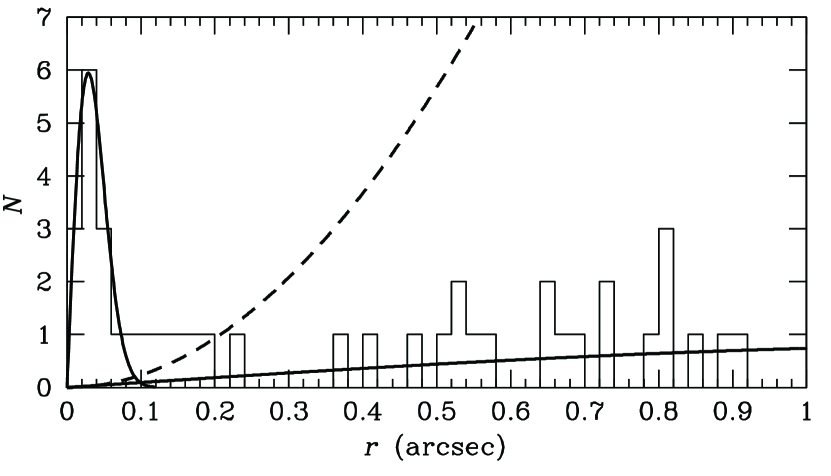
The histogram in Figure 3 shows the distribution of radio/OIR offsets $r<1^{\prime\prime}$ for all 114 radio sources with $SNR\geq 5$ in our high-resolution ($0\,\farcs 22$) image. The sharp Rayleigh distribution cutting off near $r=0\,\farcs 09$ fits the $N=14$ identifications with $m<3$ and $\langle\sigma\rangle\approx 0\,\farcs 03$. The slowly rising solid curve indicates the number of unrelated OIR objects with sky density $\rho=0.0720(114-14)/114\mathrm{~{}arcsec}^{-2}$ expected per bin of width $\Delta r=0\,\farcs 02$, and the dashed curve is their calculated cumulative distribution $N(>r)$. The observed density of unrelated OIR objects matches the calculated curves quite well for $0\,\farcs 2<r<1^{\prime\prime}$, indicating that clustering on scales $\lesssim 1\arcsec$ (i.e., $\lesssim 8\,$kpc at $z\gtrsim 1$) does not detectably increase the number of nearby OIR objects. However, there are five “unexpected” OIR objects with $0\,\farcs 09\lesssim r\lesssim 0\,\farcs 2$ where we expected only one in our sample of 114 radio sources. This discrepancy reveals that the OIR identifications of some faint radio sources may genuinely be slightly offset in position; in particular, the most intense radio emission may come from a dusty star-forming region in a merging system with patchy OIR obscuration. For example, an $r\approx 0\,\farcs 6$ (4 kpc) separation was measured between rest-frame UV and far-infrared emission peaks in the high-redshift starburst galaxy GN20 (Hodge et al., 2015). We inspected the OIR images of the five “unexpected” objects and estimate that four of the five sources in Table 2.3 with $S_{\mathrm{P}}/\sigma_{\mathrm{n}}\geq 5$ and $0\,\farcs 09<r<0\,\farcs 2$ are correctly identified.

We carried out a similar analysis to asses the reliability of sources between $3.5\leq S_{\mathrm{P}}/\sigma_{\mathrm{n}}<5$, for which there was a total of 544 sources in the relative gain-weighted beam solid angle. For a $SNR=3.5$, Equation 6 gives an rms position error of $\sigma=0\,\farcs 37$. Setting $m=3$, we estimate a total of 1.5 false detections within a search radius of $r<0\,\farcs 11$. In Table 2.3 there are 3, $3.5\leq S_{\mathrm{P}}/\sigma_{\mathrm{n}}<5$ sources with $0\,\farcs 11<r<0\,\farcs 2$ that we consider to be reliable since: one is associated with a bright $JH_{\rm NIR}=20.61$ mag galaxy, another is additionally detected at 1.4 GHz, and the third is is associated with a heavily obscured, morphologically-disturbed galaxy for which a large offset appears physical based on a visual inspection.

Figure 3.— The histogram shows the numbers $N$ of radio sources per bin of width $\Delta r=0\,\farcs 02$ with nearest OIR neighbors at angular offsets $r<1^{\prime\prime}$. The sharp Rayleigh distribution matches the observed 14 sources identified by position coincidence with $m<3$ and median $\langle\sigma\rangle\approx 0\,\farcs 03$. The broad curve is the expected differential distribution for unrelated OIR objects with sky density $\rho=0.0720\mathrm{~{}arcsec}^{-2}$, and the dashed curve is the calculated cumulative distribution $N(>r)$. It predicts one unrelated optical object will fall within $r=0\,\farcs 2$ of a $5\sigma_{\rm n}$ radio source.

Figure 4.— Examples of sources detected in our 10 GHz pilot observations. Also shown are HST/ACS $z$-band and HST/WFC3 F160W images with 10 GHz contours overlaid. Each panel is a $5\arcsec\times 5\arcsec$ cutout. Along with redshifts, 1″ scale bars are shown. The top row illustrates our ability to resolve the two cores in this merging galaxy pair at $z=1.2234$, while the bottom row illustrates our ability to detect optically invisible sources in the radio at high redshifts.

We report a total of 32 reliable identifications for radio sources detected at $\geq 3.5\sigma_{\mathrm{n}}$ significance in our full-resolution 10 GHz image. The median positional uncertainty among these 32 sources is $\langle 3\sigma\rangle\approx 0\,\farcs 1$, which is typically larger than the median measured separation between the OIR and radio positions $\langle r\rangle\approx 64\pm 11$ mas. However, there are 9 instances ($\approx 30$%) where the radio and OIR separation exceeds 3$\sigma$ by a median of $\approx 53\pm 12\,\mathrm{mas}\lesssim 0.41\pm 0.10\,\mathrm{kpc}$ at any redshift. The median distance between the radio and OIR centroids for the 9 offset identifications is $149\pm 13\,\mathrm{mas}\lesssim 1.17\pm 0.10\,\mathrm{kpc}$.

In the 1″ resolution image we report a total of 27 reliable identifications detected at $\geq 3.5\sigma$ and matched to an OIR counterpart, 6 of which are not detected in the full-resolution image. The median positional uncertainty among these 27 sources is $\langle 3\sigma\rangle\approx 0\,\farcs 3$, which is typically larger than the measured separation between the OIR and radio positions, having a median separation of $\approx 126\pm 19$ mas. In this image, the radio and OIR separation for 4 sources is found to be larger than the 3$\sigma$ positional uncertainty by a median value of $\approx 31\pm 13$ mas, or $\approx 262\pm 102$ pc at their distances. In other terms, the median distance between the radio and OIR centroids for these 4 sources is $188\pm 66$ mas, or $\lesssim 1.6\pm 0.4$ kpc at any redshift.

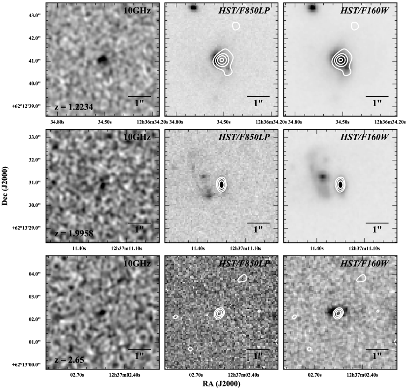
In Tables 2.3 and The GOODS-N Jansky VLA 10 GHz Pilot Survey: Sizes of Star-Forming $\mu$Jy Radio Sources, spectroscopic redshifts (Cohen et al., 2000; Wirth et al., 2004; Swinbank et al., 2004; Treu et al., 2005; Reddy et al., 2006; Barger et al., 2008; Frayer et al., 2008; Teplitz et al., 2011; D. Stern et al. in preparation; this paper) are given along with grism and photometric redshifts included in Momcheva et al. (2016). Additional notes on specific redshifts can be found in Appendix A. In every case, we provide the angular separation $r$ between the 10 GHz detection and the OIR counterpart plus the NIR magnitude ($JH_{\rm NIR}$) that is derived from some combination of $J_{125}$, $JH_{140}$ and $H_{160}$ HST/WFC3 images scaled to the $JH_{140}$ AB zeropoint as described in Momcheva et al. (2016). We present image cutouts for 3 examples of 10 GHz sources matched to HST counterparts in Figure 4, one of which illustrates how dust obscuration can cause a statistically significant offset between the radio and OIR positions.

2.3.2 A Warning About 5$\sigma_{\mathrm{n}}$ “Detections” in Sparse Images

There are 114 sources with $SNR\geq 5$ in our image covering $\Omega=3.6\times 10^{5}\mathrm{~{}arcsec}^{2}$ with $\theta_{1/2}=0\,\farcs 22$ FWHM resolution. The noise has the same angular power spectrum as the synthesized beam, so there are $N_{\mathrm{n}}\approx 8\ln(2)\Omega/(\pi\theta_{1/2}^{2})\approx 1.3\times 10^{7}$ independent noise samples in our image. The image noise amplitude distribution (Figure 5) is nearly, but not perfectly, Gaussian. If it were perfectly Gaussian, the probability that any sample would exceed $+5\sigma_{\mathrm{n}}$ is only $P(>+5\sigma_{\mathrm{n}})=2.87\times 10^{-7}$ and there would be only $N_{\mathrm{n}}P(>+5\sigma_{\mathrm{n}})\sim 4$ false radio sources stronger than $+5\sigma_{\mathrm{n}}$. However, we believe that nearly all of the 95 optically unidentified $5\sigma_{\mathrm{n}}$ sources are actually spurious for several reasons: (1) The histogram of the $SNR$s for the 95 unidentified sources is extremely steep and cuts off below $SNR=6.2$. (2) We cannot match any of these 95 sources reliably to sources in the extremely deep Spitzer/IRAC data at 3.6 or 4.5 $\mu$m within a 1″ radius using catalogs compiled from Elbaz et al. (2011), which is surprising if these sources were in fact real but within heavily obscured galaxies. (3) The 95 unidentified sources are uniformly distributed across the primary beam as one would expect for random noise; they are not concentrated toward the center of the primary beam where real sources are stronger. (4) We found a similar number (92) of sources more negative than $-5\sigma_{\mathrm{n}}$ in our high-resolution image by multiplying the image intensity units by $-1$ and running PyBDSM to find negative sources.

Figure 5.— The pixel brightness distribution of the high-resolution image uncorrected for primary-beam attenuation, over the entire 10 GHz primary beam area used for our source identifications. The bin width is a $0.05\,\mu\mathrm{Jy\,beam}^{-1}$. The dashed line is a Gaussian fit with rms $\sigma=0.572\,\mu\mathrm{Jy\,beam}^{-1}$ (i.e., the rms measured in the image out to 5% of the primary beam response). The noise in the 10 GHz image appears Gaussian and extremely well behaved.

We believe that the false $\pm 5\sigma$ “detections” in our high-resolution image are simply the result of faint non-Gaussian image fluctuations related to unedited RFI, imperfectly cleaned sidelobes, and calibration errors. The lesson here is that sources in very sparse images (many clean beam solid angles per source) cannot be trusted at the $5\sigma_{\mathrm{n}}$ level, even if the image noise looks perfectly uniform and Gaussian to the human eye.

Low-resolution images covering fewer beam solid angles or low-frequency images containing larger numbers of sources should yield more reliable $5\sigma_{\mathrm{n}}$ sources. The situation is drastically different for the case of the 1″resolution image, in which we detected a total of 15 sources with $S_{\mathrm{P}}/\sigma_{\mathrm{n}}\geq 5$ confidence and all but one is reliably matched to an optical counterpart. The single source that is not reliably matched is $r\approx 0\,\farcs 65$ from its nearest OIR counterpart. However, this same OIR counterpart (located at a redshift of $z=2.004$) is reliably matched to a radio counterpart in the $0\,\farcs 22$ resolution image and is offset by only $r\approx 0\,\farcs 093$.

2.4. Using Spectral Indices to Estimate Thermal Fractions

Table The GOODS-N Jansky VLA 10 GHz Pilot Survey: Sizes of Star-Forming $\mu$Jy Radio Sources lists the radio spectral indices $\alpha$ between 1.4 and 10 GHz of sources found by matching our 10 GHz positions with sources in the 1.4 GHz Morrison et al. (2010) catalog. Their 1.4 GHz images have $1\farcs 7$ resolution and rms noise $\sigma_{\mathrm{n}}\approx 4\,\mu\mathrm{Jy\,beam}^{-1}$. Of the 27 sources detected in the 1″-resolution image, we were able to find 1.4 GHz counterparts for 19 of them ($\approx 70$%). For the 10 GHz sources not having 1.4 GHz counterparts, Table The GOODS-N Jansky VLA 10 GHz Pilot Survey: Sizes of Star-Forming $\mu$Jy Radio Sources lists lower limits to $\alpha$ calculated using a 1.4 GHz upper limit of $S_{\mathrm{P}}<5\sigma_{\mathrm{n}}\approx 19.5\,\mu\mathrm{Jy\,beam}^{-1}$. If we assume all sources have the same non-thermal spectral index, we can use the measured spectral indices to estimate the fractional contributions from thermal emission at the rest-frame frequencies $(\nu_{\mathrm{r}}/\mathrm{GHz})=10(1+z)$ for sources having known redshifts $z$ (e.g., Klein et al., 1984; Murphy et al., 2012b). These are given in Table The GOODS-N Jansky VLA 10 GHz Pilot Survey: Sizes of Star-Forming $\mu$Jy Radio Sources, placing limits where necessary. This simple thermal decomposition is sensitive to the estimated non-thermal spectral index, assumes that the free-free emission is optically thin at rest-frame frequencies $(\nu_{\rm r}/{\rm GHz})\gtrsim 1.4(1+z)$ (e.g., Murphy et al., 2010b), and that there is an insignificant contribution of both anomalous microwave emission at $\sim$33 GHz (e.g., Murphy et al., 2010a) and thermal dust emission in the rest frequency range $10\lesssim\nu\lesssim 40$ GHz. We took the non-thermal spectral index to be $\alpha_{\rm NT}=-0.85$, which is the average non-thermal spectral index found among the 10 star-forming regions studied in NGC 6946 by Murphy et al. (2011b) and very similar to the average value found by Niklas et al. (1997, $\langle\alpha_{\rm NT}\rangle=-0.83$ with an rms scatter of $\sigma=0.13$) globally for a sample of 74 nearby galaxies. To those sources having measured spectral indices $\alpha>\alpha_{\rm NT}=-0.85$ we assigned non-thermal indices $\alpha_{\mathrm{NT}}=\alpha-0.1$.

Figure 6.— The redshift distribution of all 38 unique sources detected in the full-resolution and/or 1″ tapered 10 GHz images with $S_{\mathrm{P}}\geq 3.5\sigma_{\mathrm{n}}$ and confirmed by having OIR counterparts. Their median redshift is $\langle z\rangle=1.24\pm 0.15$. An excess of sources (7 out of 38) are found in the narrow range of $1.9958\leq z\leq 2.0180$, and are likely members of an over-density traced by SMGs, optically-faint radio sources, and other star-forming galaxies (Chapman et al., 2009).

3. Results and Discussion

In this section we present the results for a flux-limited sample of galaxies from this pilot X-band imaging program of GOODS-N, taking advantage of both the high angular resolution delivered by the VLA A-configuration, along with its centrally concentrated core of dishes, allowing us to make images with various $(u,v)$-weightings to improve the brightness temperature sensitivity of the data. As stated in 2.2, the inclusion of the C-configuration data with our imaging helps to fill in the hole in the $(u,v)$-plane left by the A-configuration data alone that, if not accounted for, will result in underestimated angular sizes and integrated flux densities of extended sources even in the 1″ and 2″ tapered images.

3.1. Redshift Distributions

The $0\,\farcs 22$ full-resolution 10 GHz image contains 32 reliable sources at $\geq 3.5\sigma_{\rm n}$ having OIR counterparts with measured redshifts. Their median redshift is $\langle z\rangle=1.24\pm 0.16$. The 1″-resolution image contains 27 sources with OIR counterparts and measured redshifts. The median redshift of these sources is slightly lower: $\langle z\rangle=1.01\pm 0.16$, most likely because the 1″ tapered image is less sensitive to point sources but more sensitive to extended sources, which will tend to be at lower redshifts. Figure 6 shows the redshift distribution for all 38 unique sources detected in the full-resolution and/or 1″ tapered images. The median redshift of all sources with OIR counterparts is $\langle z\rangle=1.24\pm 0.15$. Figure 6 also shows an excess of sources (7 out of 38) having redshifts in the narrow range spanning $1.9958\leq z\leq 2.0180$. These sources are likely members of an over-density traced by sub-mm galaxies (SMGs), optically-faint radio sources, and other star-forming galaxies (Chapman et al., 2009). In fact, at least 6 of the 38 unique 10 GHz-detected sources reported here are 850 $\mu$m-detected SMGs (Pope et al., 2005; Chapman et al., 2009), 4 of which appear to be members of this $z\approx 2$ over-density.

Figure 7.— The distribution of deconvolved source FHWM major axes $\theta_{\mathrm{M}}$ for all 32 sources detected in the full-resolution image. The corresponding effective radii $r_{\mathrm{e}}$ are marked on the upper abscissa. The weighted median angular size is $\langle\theta_{\mathrm{M}}\rangle=167\pm 32$ mas and the weighted rms scatter in $\theta_{\mathrm{M}}$ is 91 mas. The corresponding median effective radius is $\langle r_{\mathrm{e}}\rangle=69\pm 13$ mas and the rms scatter in $r_{\mathrm{e}}$ is 38 mas.

Figure 8.— The FWHM major-axis linear sizes of all 32 detected sources plotted against redshift. The corresponding effective radii ($r_{\rm e}$) are marked along the right ordinate. The FWHM linear sizes have a weighted median $1.3\pm 0.28$ kpc and a weighted rms scatter $\approx 0.79$ kpc. The corresponding effective radii $r_{\rm e}$ have a weighted median $509\pm 114$ pc and a weighted rms scatter $\approx 324$ pc. No obvious evolution in 10 GHz radio size is seen with redshift.

3.2. The Size Distribution of $z\sim 1$ Star-Forming Disks

Radio astronomers traditionally fit elliptical Gaussians to sources on images and specify source sizes by their deconvolved major and minor FWHM axes $\theta_{\mathrm{M}}$ and $\theta_{\mathrm{m}}$. However, the radio brightness distributions of star-forming spiral galaxies are better approximated by optically thin exponential disks, and OIR astronomers often characterize the size of a disk by the effective radius $r_{\rm e}$ that encloses half of the total flux density of the deprojected disk. Appendix B shows analytically that these two size measures are related by

$$\theta_{\rm M}\approx 2.430\,r_{\rm e}~{},$$ (11)

which we use to compare our radio disk sizes to OIR sizes in the literature.

The major radio-astronomy image analysis packages (e.g., AIPS, CASA) make Gaussian but not exponential fits. These fitting routines are not easily described analytically, so we performed numerical simulations which show that Gaussian and exponential fits yield comparable results for both deconvolved sizes and peak brightness-to-integrated flux density ratios $S_{\mathrm{P}}/S_{\mathrm{I}}$ (Appendix C), at least for sources with $r_{\mathrm{e}}\lesssim\theta_{1/2}$.

The distribution of the deconvolved angular sizes for the 32 reliable 10 GHz detections listed in Table 2.3 is plotted in Figure 7. Among these, the major axes of 6 sources ($\approx 20$%) are confidently resolved at $\geq 2\sigma_{\phi_{\rm M}}$ significance (see §2.3), and are identified in Table 2.3. To determine the typical source size among the entire population of sources, we calculate a weighted median. For each source size, the weight is inversely proportional to the solid angle in which it could have been detected, limited either by $SNR$ or by the area within the 5% primary beam cutoff. The constant of proportionality is set such that a source that could be detected anywhere within the survey area has weight $w_{\rm i}=1$, but any constant of proportionality would give the same result. This weight is designed to exactly compensate for the fact that weak extended sources could be seen only in a fraction of the full survey field. Our weighted source size distribution should be representative of a sample that was uniformly selected, unbiased by angular size, over the entire survey area.

The weighted median deconvolved source FWHM is $\langle\theta_{\mathrm{M}}\rangle=167\pm 32$ mas, and the weighted rms size scatter is $\approx 91$ mas. The corresponding weighted median effective radius is $\langle r_{\mathrm{e}}\rangle=69\pm 13$ mas, and the weighted rms scatter in $r_{\mathrm{e}}$ is $\approx 38\mathrm{\,mas}$. Using the measured redshifts of these resolved sources, we plotted their linear sizes as a function of redshift in Figure 8. The weighted median FWHM major axis linear diameter of these sources is $\langle\theta_{\rm M}\rangle=1.2\pm 0.28$ kpc, and $\theta_{\mathrm{M}}$ has a weighted rms scatter of $\approx 0.79\mathrm{\,kpc}$. The corresponding weighted median effective linear radius is $\langle r_{\rm e}\rangle=509\pm 114$ pc, and the rms scatter in $r_{\mathrm{e}}$ is $\approx 324\mathrm{\,pc}$. There is no obvious indication of linear size evolution with redshift.

3.2.1 Comparison with Other Radio and mm/sub-mm Sizes

Using a deep VLA 3 GHz image of the Lockman Hole made with $\theta_{1/2}=0\,\farcs 66$ resolution, Condon et al. (2016, in prep) found a preliminary median source size $\theta_{\mathrm{M}}\approx 300\pm 100$ mas among their detections. Although slightly larger than the 10 GHz sizes reported here, they are actually quite consistent since we expect the 3 GHz radio size to be slightly larger than at 10 GHz for two reasons: (1) The lower-energy relativistic electrons emitting at 3 GHz may diffuse farther because they have longer synchrotron lifetimes. For rigidity-dependent diffusion of cosmic-rays (CRs), where the magnetic rigidity scales as $R^{0.75}$ as measured for CR electrons and protons around 30 Dor (Murphy et al., 2012a), 3 GHz emitting CR electrons will diffuse $\approx 25$% further than 10 GHz emitting CR electrons. (2) Thermal emission confined to the star-forming regions contributes a smaller fraction of the total flux density at 3 GHz.

However, the measured radio sizes of our 10 GHz-selected sources are significantly smaller than the 3 GHz sizes reported by Miettinen et al. (2017) for a sample of 115 known SMGs in the COSMOS field. Using sensitive ($\sigma_{\mathrm{n}}\approx 2.4\,\mu\mathrm{Jy\,beam}^{-1}$) 3 GHz images from the VLA-COSMOS 3 GHz Large Project (Smolčić et al. 2016, in press), they found a median source size $\theta_{\mathrm{M}}\approx 590\mathrm{\,mas}$ and an rms size scatter of 420 mas. Given the redshifts of their sources, their median angular size corresponds to a median linear size $\approx 4.5\mathrm{\,kpc}$. That is also close to the median 1.4 GHz size for a sample of 12 SMGs reported by Biggs & Ivison (2008, i.e., $640\pm 100$ mas), which corresponds to a linear size of $5$ kpc given the redshifts of their sources. In contrast, our measured sizes are in much better agreement with the ALMA sizes from Ikarashi et al. (2015) and Simpson et al. (2015), who report median sizes of $200\pm 50$ mas ($1.6\pm 0.14$ kpc) at 1.1 mm and $300\pm 40$ mas ($2.4\pm 0.2$ kpc) at 870 $\mu$m, respectively. Thus, while our radio sizes are not for a sample of SMGs, which may be different from the more typical star-forming galaxies selected at 10 GHz, it is interesting to find that our radio sizes are compatible with the high-resolution dust-emitting sizes of SMGs.

One might expect sub-mm sizes to be different from the radio emitting sizes given the different selection criteria. SMGs selected at sub-mm wavelengths may be intrinsically different from star-forming galaxies selected by synchrotron or free-free emission at cm wavelengths because the sub-mm galaxies have no $K$-correction and thus are intrinsically more luminous and at higher redshifts than cm-selected galaxies. Furthermore, even for the same galaxy population, the size measured at sub-mm wavelengths may be different (larger) than the size measured at cm wavelengths because the submm size is that of the cold cirrus dust distribution while the cm size is closer to that of the current star formation.

Figure 9.— The ratio of 10 GHz-to-HST/WFC3 F160W (van der Wel et al., 2014) continuum effective radii plotted as a function of NIR magnitude for all 32 sources reliably detected in the full-resolution radio image. On average, the 10 GHz sizes are $0.14\pm 0.05$ times the rest-frame optical size (not corrected for extinction), and the size ratios have an rms scatter of 0.21, indicating that the star formation in our sample of $z\sim 1$ star-forming galaxies is centrally concentrated.

Figure 10.— Left: Measured ratios $S_{\mathrm{P}}/S_{\mathrm{I}}$ of peak brightness-to-integrated flux densities for all sources detected in our $0\,\farcs 22$-resolution image versus the deconvolved disk effective radius $r_{\mathrm{e}}$ in units of arcsec. The solid curve was calculated from Equation C6 for a circular (face-on) exponential disk. The dashed curve was calculated from Equation C7 for the median inclination angle $i=60^{\circ}$ [$\cos(i)=0.5$] of randomly oriented disks, and the dotted curve corresponds to a nearly edge-on disk with $\cos(i)=0.25$. The data points should lie between the solid and dotted curves and be centered around the dashed curve. Right: The same as the left panel, except that the abscissa units are kpc instead of arcsec for sources with measured redshifts.

3.2.2 Comparing Radio, H$\alpha$, and Optical Sizes

We also compared our star-forming galaxy disk sizes with those reported by Nelson et al. (2016), which are based on stacking resolved H$\alpha$ and H$\beta$ emission-line images from the 3D-HST survey. By comparing their H$\alpha$ and H$\beta$ galaxy images, these authors could apply an extinction correction to their H$\alpha$ images before fitting for the effective radius. This extinction correction significantly lowers the measured sizes because it multiplies the inferred star-formation rates in the central $r<1$ kpc of galaxies with $9.8<\log(M/M_{\odot})<11.0$ by a factor of $\approx 6$. The average extinction-corrected H$\alpha$ radial profile of these galaxies declines by a factor of $\approx 100$ between the center and $r\approx 2$ kpc, which corresponds to an effective radius of $\langle r_{\mathrm{e}}({\mathrm{H}}\alpha)\rangle\approx 0.73$ kpc. Before making the extinction correction, Nelson et al. (2012) had reported a median H$\alpha$ effective radius $\langle r_{\mathrm{e}}\rangle=4.2\pm 0.1$ kpc for a sample of 57 strongly star-forming galaxies in the same mass range. Thus, the uncorrected $r_{\mathrm{e}}$ is $\approx 6\times$ larger than the corrected $r_{\mathrm{e}}$. The effective radius of the extinction-corrected H$\alpha$ radial profiles is not significantly larger than our weighted median $\langle r_{\mathrm{e}}\rangle\approx 0.51\pm 0.11\mathrm{\,kpc}$ with rms scatter 0.32 kpc at 10 GHz and is much more consistent with the radio sizes reported here than with others in the literature. The small difference between our measured sizes and the extinction-corrected H$\alpha$ sizes might result from underestimating extinctions in the centers of the most massive galaxies in Nelson et al. (2016).

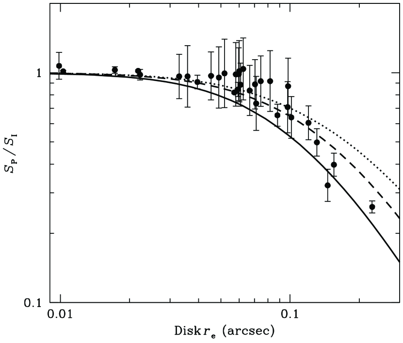
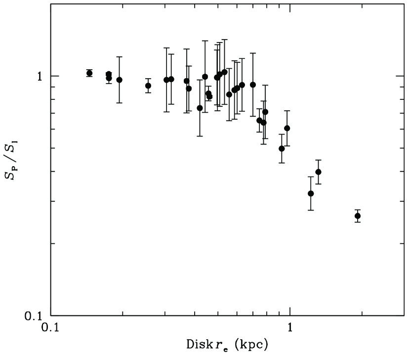
The effect of extinction may also be contributing to what is found in Figure 9, which plots the ratio of the 10 GHz effective radius to the rest-frame optical continuum $r_{\mathrm{e}}$ reported by van der Wel et al. (2014) as a function of NIR magnitude. The rest-frame optical data used were not corrected for extinction. The star-forming disks measured at 10 GHz, which are similar to the extinction-corrected H$\alpha$ sizes reported by Nelson et al. (2016), are significantly smaller than the uncorrected rest-frame optical continuum sizes. The median 10 GHz-to-F160W size ratio is $0.14\pm 0.05$, and the size ratios have an rms scatter of 0.21. Consequently, the star formation appears to be centrally concentrated in this sample of $z\sim 1$ galaxies.

Here, we have converted the decononvolved Gaussian fits to the radio sizes to half-light radii $r_{e}$ assuming the conversion for exponential profiles discussed in Appendix B. The HST/WFC3 sizes from van der Wel et al. (2014), $r_{\rm e}{\rm(F160W)}$, were derived from Sérsic (1963, 1968) profile model fitting, and thus may not exactly match exponential fits (i.e., Sérsic index $n=1$) on a galaxy-by-galaxy basis. Moreover, the HST/WFC3 F160W filter measures optical rest-frame starlight at the mean redshift of our 10 GHz-selected sample, and thus may not simply reflect the distribution of optically-bright star formation in each galaxy. Nevertheless, it seems clear from Figure 9 that the 10 GHz radio (and H$\alpha$) sizes are uniformly and significantly smaller than the optical galaxy sizes derived from the CANDELS HST images not corrected for extinction. Accordingly, similar to what has been shown for H$\alpha$ sizes, extinction may be playing a role.

3.2.3 $S_{\mathrm{P}}/S_{\mathrm{I}}$ Ratios of Randomly Oriented Thin Disks

If star-forming galaxies are randomly oriented, transparent, thin, and circular exponential disks at radio wavelengths, they should appear elliptical on the sky, with minor axes shortened by $\theta_{\mathrm{m}}/\theta_{\mathrm{M}}=\cos(i)$, where $i$ is the inclination angle between the disk normal and the line of sight. However, the minor axes $\theta_{\mathrm{m}}$ of many galaxies in Table 2.3 are not resolved, which necessitates another way to check this hypothesis. One way is to use the ratio $S_{\rm P}/S_{\rm I}$ of peak brightness to integrated flux density, a quantity that depends on both $\theta_{\mathrm{M}}$ and $\theta_{\mathrm{m}}$, and is available for all galaxies. The dependence of $S_{\mathrm{P}}/S_{\mathrm{I}}$ on galaxy size and inclination is derived in Appendix C. The results are shown as functions of $r_{\mathrm{e}}$ in Figure 10. They are consistent with most of our radio sources being randomly oriented, thin, circular exponential disks.

Figure 11.— The median spectral index among all 19, 1.4 GHz detected sources is $\langle\alpha_{\rm 1.4\,GHz}^{\rm 10\,GHz}\rangle\approx-0.74\pm 0.10$ with a standard deviation of 0.35. Including the additional 8 sources for which there are only upper limits on the 1.4 GHz flux density flattens the median spectral index of our full flux-limited sample selected at 10 GHz to $\langle\alpha_{\rm 1.4\,GHz}^{\rm 10\,GHz}\rangle\gtrsim-0.61$.

3.3. Spectral Indices and Thermal Fractions

Using the 1″ and 2″ resolution images, which bracket the $1\,\farcs 7$ resolution of the Morrison et al. (2010) 1.4 GHz image, we are able to measure radio spectral indices with nearly matched resolution (see Table The GOODS-N Jansky VLA 10 GHz Pilot Survey: Sizes of Star-Forming $\mu$Jy Radio Sources). Among the 19 sources with 1.4 GHz counterparts, the median observed spectral index between 1.4 and 10 GHz is $\langle\alpha_{\rm 1.4\,GHz}^{\rm 10\,GHz}\rangle\approx-0.74\pm 0.10$ with a standard deviation of $\sigma_{\alpha_{\rm 1.4\,GHz}^{\rm 10\,GHz}}\approx 0.35$. This median is consistent with what is measured for star-forming galaxies in the local universe (e.g., Condon, 1992). However, by including the 8 sources (30% of our detections) having only 1.4 GHz upper limits, the median flattens significantly to $\gtrsim-0.61$. The large number of sources without 1.4 GHz counterparts is not that surprising since, as stated in §2.2, for a source with spectral index of $-0.7$ the 10 GHz images are $\approx 2$ times more sensitive than the 1.4 GHz image of Morrison et al. (2010). Even so, it appears that there is a significant fraction of sources at $z\gtrsim 1$ having somewhat flat spectral indices, suggesting that higher-frequency radio measurements may indeed be more sensitive to free-free emission and consequently a more robust measure for the current star formation activity in such systems. Figure 11 plots the measured spectral indices agains redshift, for which there is no clear trend.

As discussed in §2.4, by assuming a fixed, non-thermal spectral index for each source, we can use the measured spectral indices to estimate the fractional contributions from thermal emission at the rest-frame frequency $(\nu_{\rm r}/{\rm GHz})=10(1+z)$ (e.g., Klein et al., 1984; Murphy et al., 2012b), which are listed in Table The GOODS-N Jansky VLA 10 GHz Pilot Survey: Sizes of Star-Forming $\mu$Jy Radio Sources. These estimates additionally assume that the observed 10 GHz emission is in fact powered by star formation. For the 19 sources having 1.4 GHz counterparts the median redshift corresponds to a rest-frame frequency of $\approx 20$ GHz for which we estimate a median thermal fraction of $26\pm 0.09$% with an rms scatter of 31%. If we additionally include the 8 sources for which we only have upper limits at 1.4 GHz, the median redshift also corresponds to a rest-frame frequency of $\approx 20$ GHz and places a lower limit on the median thermal fraction of $\gtrsim$48%. While we have assumed a non-thermal spectral index of $-0.85$, one caveat is that spectral steepening in the rest-frame near 20 GHz (e.g., from increased synchrotron and inverse-Compton losses), which is extremely difficult to measure, could result in underestimates of the thermal fractions.

3.3.1 Comparison with Previous Deep X-band Imaging

Our 2″ tapered image can be compared with the X-band image of Richards et al. (1998). They detected 29 sources stronger than 5$\sigma_{\mathrm{n}}$ in a field of radius of 4$\farcm$6 (truncated at $\approx 8$% of the primary beam response) in their 8.5 GHz image centered on the Hubble Deep Field. For the original VLA system, the primary beam FWHM at 8.5 GHz is $\approx 5\farcm 2$. Their 8.5 GHz VLA data from the A, BnA, C, DnC, and D configurations respond to sources up to 10″ in size. The bulk of their observing time was in the C configuration, and their final image had resolution $\theta_{1/2}\approx 3\farcs 5$ and rms noise $\sigma_{\mathrm{n}}\approx 1.8\,\mu\mathrm{Jy\,beam}^{-1}$, corresponding to a brightness-temperature sensitivity $\sigma_{\mathrm{n}}\approx 2.5\,\mathrm{\,mK}$. This is similar to our $\sigma_{\mathrm{n}}=1.5\,\mu\mathrm{Jy\,beam}^{-1}$ rms, which scales to $\approx 1.7\,\mu\mathrm{Jy\,beam}^{-1}$ at 8.5 GHz for a source with typical spectral index $\alpha=-0.7$, and a 4.7 mK brightness temperature rms achieved in our 2″ image.

In our 2″ resolution image we detected a total of 14 sources with $S_{\mathrm{P}}/\sigma_{\mathrm{n}}\geq 5$ that are reliable (i.e., the same 5$\sigma_{\mathrm{n}}$ sources we consider to be reliable in our 1″-resolution image). Given the ratio of primary beam solid angles $\Omega_{\mathrm{10GHz}}/\Omega_{\mathrm{8.5GHz}}=0.67$ and sensitivities at the two frequencies, we would expect them to detect $\approx 50$% more sources (i.e., $\approx 21$ sources). This prediction is slightly more than 1$\sigma$ smaller than what counting errors would suggest. However, if we were to include the single 5$\sigma$ detection from our 2″ tapered image that is considered unreliable, or exclude the four $S_{\mathrm{P}}>5\sigma_{\mathrm{n}}$ sources in the Richards et al. (1998) sample that were not matched to optical counterparts, our numbers do in fact agree to within 1$\sigma$ of the counting errors.

3.4. A Revised Redshift and Spectral Energy Distribution Analysis for VLA J123642$+$621331

We detected the radio source VLA J123642$+$621331 described by Waddington et al. (1999) as a compact [$r_{\rm e}{\rm(F160W)}\approx 0\,\farcs 2$] star-forming galaxy containing an AGN. The 10 GHz flux density measured in our 1″  tapered image is consistent with the 8.5 GHz flux density reported by Richards et al. (1998, 1999), being $\approx 70\,\mu$Jy. The source is detected in both our $0\,\farcs 22$ and $1\arcsec$ resolution images, having deconvolved major axes of $42\pm 23$ mas and $0\,\farcs 65\pm 0\,\farcs 06$, respectively, suggesting a compact core and consistent with the upper limit $<0\,\farcs 1$ reported by Richards et al. (1998) in their lower signal-to-noise 0 $\farcs$2 resolution image. VLA J123642$+$621331 was resolved by high resolution (0 $\farcs$15) 1.4 GHz VLA+MERLIN observations (Muxlow et al., 1999), which showed that 10% of the flux density resides in an extended component lying to the east of an unresolved core. The unresolved, compact core was additionally detected by the European VLBI Network (EVN) at 1.6 GHz, providing an upper limit on the core size of 20 mas and corresponding 1.6 GHz brightness temperature of $T_{\rm b}>2\times 10^{5}$ K (Garrett et al., 2001), indicating that the core emission is dominated by an AGN (Condon et al., 1991).

Figure 12.— Left: A portion of the HST/WFC3 G140 grism spectrum of VLA J123642+621331, showing the emission feature identified as the [Oiii] doublet. Right: A portion of the Keck/MOSFIRE spectrum. The red tickmarks indicate the predicted wavelengths of the [Nii] and H$\alpha$ emission lines, based on the redshift fit to the WFC3 grism spectrum ($z_{\rm[O\textsc{iii}]}=2.015)$. The broad, blended H$\alpha$+[Nii] complex seems to be redshifted slightly with respect to these predictions, with a visual estimate ($z=2.018\pm 0.003$) indicated by the dashed blue lines.

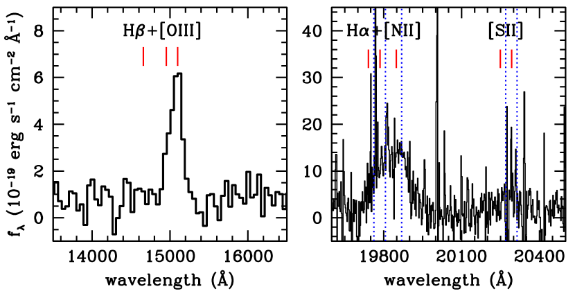
Waddington et al. (1999) reported a redshift $z=4.424$ for this source, on the basis of a single emission line detected with Keck/LRIS at 6595 Å interpreted to be Lyman $\alpha$, apparently offset by about $1^{\prime\prime}$ from the optical galaxy position. However, more recent multiwavelength photometric data in the GOODS-N field suggest that the galaxy may instead have a lower redshift, due to faint but significant detection in the GOODS HST/ACS $B$-band (F435W) image, as well as mid- to far-infrared photometry (and sub-mm upper limits) that seem inconsistent with $z=4.4$. A slitless spectrum from the HST/WFC3 G140 grism (GO-11600, PI Benjamin Weiner) detects a strong, slightly asymmetric line (Figure 12, left), which we interpret as the blended [Oiii] 4959,5007 Å doublet, with no detectable H$\beta$ [$f(5007)/f({\rm H}\beta)>4.6$ at $2\sigma$]. A constrained two-Gaussian fit to the extracted grism spectrum yields a redshift $z_{\rm[O\textsc{iii}]}=2.015$.

We then obtained a $K$-band spectrum of VLA J123642$+$621331 with MOSFIRE on the Keck 1 telescope on UT 2014 April 13 under photometric conditions, using a slit width of 0 $\farcs$7, for a total exposure time of 84 minutes. The data were reduced using the standard MOSFIRE data reduction pipeline (version 2014.06.10). Figure 12 (right) shows a 2″ wide extraction for a portion of the spectrum. A broad ($\approx 175$ Å) feature is detected, centered at approximately 19825 Å. We interpret this as a blend of broad H$\alpha$ plus [Nii]. The complex appears to be slightly offset from the wavelengths predicted based on the fit to [Oiii] in the grism data. We cannot formally fit the lines, but we estimate $z=2.018$ from the MOSFIRE spectrum.

This redshift difference with respect to that from [Oiii] ($\Delta z=0.003$) is easily consistent with typical uncertainties in HST/WFC3 grism spectral measurements (Momcheva et al., 2016). The 6595 Å line reported by Waddington et al. (1999) would not correspond to any emission features commonly seen in distant galaxies or AGN, and it may be a serendipitous detection of another faint, nearby galaxy at a different redshift (perhaps indeed Lyman $\alpha$), or it could be spurious. The apparently broad H$\alpha$ emission, high [Oiii]/H$\beta$ ratio, and perhaps strong [Nii] all suggest that an AGN dominates the optical rest-frame nebular line emission. This IR-luminous, radio-loud AGN could be another member of an over-dense structure at $\langle z\rangle=1.99$ traced by sub-mm-, radio-, and UV-selected star-forming galaxies (Chapman et al., 2009).

The WFC3 grism spectrum of J123642$+$621331 was also analyzed by Ciardullo et al. (2014), who derived $z=2.018$, and in the 3D-HST catalog of Momcheva et al. (2016), who derived $z=2.012\pm 0.002$ (68% confidence).

Using a compilation of radio-to-optical data in the literature, we fit the full spectral energy distribution of VLA J123642$+$621331, which is shown in Figure 13. The radio data were not used to constrain the fit, which assumes the standard far-infrared–radio correlation and a typical radio spectrum with $S_{\nu}\propto\nu^{-0.8}$. The OIR data were fit with the updated Bruzual & Charlot (2003) stellar templates having an exponentially declining star formation history with a characteristic timescale of $\tau=0.1$ Gyr and being extincted by an $A_{V}=2.4$ assuming a local starburst attenuation law (Calzetti et al., 2000). The mid-infrared emission powered by hot dust was fit by a power law, while the far-infrared is fit by a cold dust model (i.e., a modified black body with $\beta_{\rm dust}=1.9$). The best-fit spectral energy distribution is characterized by a stellar mass of $M_{*}=2.4\times 10^{10}\,M_{\odot}$, a stellar mass fraction of $f_{*}=0.4$, an IR luminosity of $L_{\rm IR}=2.3\times 10^{12}\,L_{\odot}$, and a dust temperature of $T_{\rm dust}=70\,$K.

Figure 13.— The best-fit radio-to-optical spectral energy distribution of VLA J123642$+$621331. Data used in the fitting was taken from the literature: OIR data – CANDLES GOODS-N multiwavelength catalog (G. Barro et al., 2016, in preparation); Spitzer and Herschel far-infrared data (Magnelli et al. 2011; Teplitz et al. 2011; H. Inami et al., 2016, in preparation); SCUBA sub-mm data (Borys et al., 2003; Pope et al., 2005); 1.16 mm AzTEC$+$MAMBO data (Penner et al., 2011); 2mm GISMO data (Staguhn et al., 2014). The radio data were not used to constrain the fit, which assumes the standard far-infrared–radio correlation and a typical radio spectrum with $S_{\nu}\propto\nu^{-0.8}$. The best-fit spectral energy distribution is characterized by a stellar mass of $M_{*}=2.4\times 10^{10}\,M_{\odot}$, a stellar mass fraction of $f_{*}=0.4$, an infrared (IR; $8-1000\,\mu$m) luminosity of $L_{\rm IR}=2.3\times 10^{12}\,L_{\odot}$, and a dust temperature of $T_{\rm dust}=70\,$K, which is extremely hot even when compared to local AGN (e.g., Spinoglio et al., 1995; Andreani et al., 2002). The measured logarithmic far-infrared–radio ratio of $q=1.19$ has a factor of $\approx 30$ times (i.e., 5.6$\sigma$) more radio emission compared to the locally measured value for star-forming galaxies, also indicating the presence of an AGN.

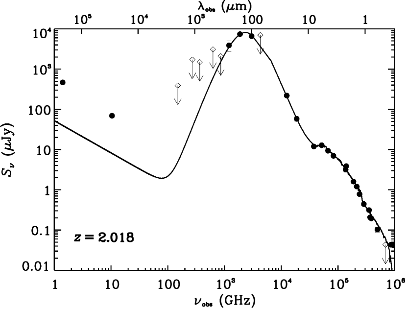
Taking the observed 1.4 GHz flux density of 494.2 $\mu$Jy (Morrison et al., 2010) and the measured 1.4-to-10 GHz spectral index of $-1.02$ in Table The GOODS-N Jansky VLA 10 GHz Pilot Survey: Sizes of Star-Forming $\mu$Jy Radio Sources, the corresponding K-corrected logarithmic IR–radio ratio is $q_{\rm IR}=1.19$, which exhibits a factor of $\approx 30$ (i.e., 5.6$\sigma$) radio excess compared to the locally measured value of 2.64 (Bell, 2003), and thus strongly suggests the presence of an AGN. The far-infrared emission peak at 30$\,\mu$m in the rest frame implies a remarkably high dust temperature, similar to that seen in a minority of 3C sources (e.g., Spinoglio et al., 1995; Andreani et al., 2002), and suggests that the AGN dominates the bolometric luminosity of this source.

We have presented exquisite multiwavelength data on a radio galaxy at $z=2.018$. The change in redshift for this source from the previously claimed $z=4.424$ highlights the dangers in single line redshift determination, especially when the ancillary photometry is poor; for example, similar criteria have been used to claim the detection of a $z=4.88$ radio galaxy (Jarvis et al., 2009). With the accurate spectral energy distribution we have of VLA J123642$+$621331, we can predict the colors of $z>2$ radio galaxies that will be detected in forthcoming wide-area radio surveys such as the Evolutionary Map of the Universe (EMU; Norris et al., 2011, 1.4 GHz; 5$\sigma\approx 50\,\mu$Jy; $\theta_{1/2}\approx 10\arcsec$) and VLA Sky Survey (VLASS; Murphy & VLASS Survey Science Group, 2015, 3 GHz; 5$\sigma\approx 345\,\mu$Jy; $\theta_{1/2}\approx 2.5\arcsec$). Sources like VLA J123642$+$621331 at $z\sim 3$ would have flux densities of 0.45 $\mu$Jy in the $H-$band, 0.9 $\mu$Jy in the $K-$band and $S_{\rm 1.4\,GHz}$/$S_{K}$ ratios of $\approx 170$. It would therefore be challenging to detect their counterparts in wide-field NIR surveys such as those that will be undertaken with EUCLID. At $z\sim 5$, which is the limit at which such a source would be detected in the EMU survey, it would be 60 nJy in the $H-$band, 130 nJy in the $K-$band and 0.5 $\mu$Jy at 3.6 $\mu$m. These are challenging sensitivities to achieve, partly due to source confusion in the latter case. Confirming the redshifts of such sources will instead benefit from spectroscopy at sub-mm/mm frequencies since the equivalent $z\sim 5$ source would be 150 $\mu$Jy and 80 $\mu$Jy at 850 $\mu$m and 1.2 mm respectively, which is achievable with ALMA and NOEMA. In summary, the low stellar mass of VLA J123642Q$+$621331 suggests that it will be difficult to obtain OIR spectroscopic redshifts of high-redshift ($z>3$) radio galaxy candidates and mm spectroscopy of [Cii] may be the most compelling approach.

4. Conclusions

In this paper we presented results from our pilot VLA 10 GHz survey of GOODS-N, aimed at resolving compact starbursts in the redshift range between $1\lesssim z\lesssim 3$. This deep, single pointing image reaches an rms noise $\sigma_{\mathrm{n}}=572\mathrm{\,nJy\,beam}^{-1}$ and has $\theta_{1/2}=0\,\farcs 22$ resolution. Our conclusions can be summarized as follows:

• The median redshift among the 38 unique sources detected in the full-resolution and/or 1″ tapered 10 GHz images confirmed by having OIR counterparts is $\langle z\rangle=1.24\pm 0.15$.

• Of the 32 sources reliably detected at 10 GHz in the image with $0\,\farcs 22$ FWHM resolution, the weighted median of their deconvolved FHWM major axes is $\langle\theta_{\rm M}\rangle=0\,\farcs 17\pm 0\,\farcs 03$, and the weighted rms size scatter is $\approx 0\,\farcs 09$. The weighted median linear major-axis FWHM size of these sources is $\langle\theta_{\rm M}\rangle=1.2\pm 0.28$ kpc, and the weigthed rms scatter in the linear sizes is $\approx 0.79$ kpc. In units of effective radius $r_{\rm e}$, these values are equal to $\langle r_{\rm e}\rangle=69\pm 13\mathrm{\,mas\,}/508\pm 114\mathrm{\,pc}$ with corresponding rms scatter $\approx 38\mathrm{\,mas}/324\mathrm{\,pc}$. We found no evidence for evolution in radio size with redshift. Our 10 GHz source sizes are significantly smaller than lower-frequency radio sizes reported in the literature, but they appear to agree with high-resolution mm/sub-mm sizes that trace dust emission and with extinction-corrected H$\alpha$ sizes. This result indicates that star formation near the cosmic star formation rate peak largely occurs in relatively compact regions within galaxies.

• For the detections in our $1\arcsec$-resolution 10 GHz image that have 1.4 GHz counterparts, we measured a median spectral index $\langle\alpha_{\rm 1.4\,GHz}^{\rm 10\,GHz}\rangle\approx-0.74\pm 0.10$, and the spectral indices have an rms scatter $\sigma_{\alpha_{\rm 1.4\,GHz}^{\rm 10\,GHz}}\approx 0.35$, consistent with what is measured for star-forming galaxies in the local universe and the measurement errors in $\alpha$. Adding the sources with only upper limits to their 1.4 GHz flux densities places a lower limit on the median spectral index $\langle\alpha_{\rm 1.4\,GHz}^{\rm 10\,GHz}\rangle\gtrsim-0.61$, indicating that a signifiant fraction of $z\gtrsim 1$ sources selected at 10 GHz have relatively flat spectra, which may indicate that free-free emission contributes significantly and makes their total flux densities robust measures of the current star formation activity in such sources.

• Using the spectral indices measured for detections in the $1\arcsec$-resolution 10 GHz image having 1.4 counterparts, and assuming a typical non-thermal spectral index for each source (i.e., $\alpha_{\rm NT}\approx-0.85$), we estimate a median thermal fraction of $26\pm 0.09$% with a standard deviation of 31% for a median rest-frame frequency of $\approx 20$ GHz. Additionally including the 8 sources having only upper limits for the 1.4 GHz flux densities places a lower limit on the median thermal fraction of $\gtrsim$48% at the same median rest-frame frequency of $\approx 20$ GHz.

• Using a combination of HST/WFC3 G140 grism and MOSFIRE spectroscopy, we measured a new redshift for VLA J123642$+$621331 of $z=2.018$ that is significantly lower than the $z=4.424$ previously reported in the literature. Using data from the radio into into the optical, the best-fit spectral energy distribution is characterized by a stellar mass of $M_{*}=2.4\times 10^{10}\,M_{\odot}$, a stellar mass fraction of $f_{*}=0.4$, an IR luminosity of $L_{\rm IR}=2.3\times 10^{12}\,L_{\odot}$, and an extremely hot dust temperature of $T_{\rm dust}=70\,$K .

Appendix A Notes on Specific Redshifts

The source in Table 2.3 with coordinates $\alpha=12^{\mathrm{h}}36^{\mathrm{m}}44\fs 110,\delta=+62\arcdeg 12\arcmin 44\farcs 81$ (also listed in Table 2) has a grism-based redshift of $z=1.676$ reported by Momcheva et al. (2016), with a 68% confidence interval of 1.631 to 1.705. A deeper inspection of the 3D-HST data products suggest that this redshift estimate is primarily derived from the galaxy photometry, with little contribution from the grism data. The extracted spectrum is truncated and covers only 6% of the normal grism spectral range, and no obvious emission or absorption features are detected. The corresponding photometric redshift provided by Momcheva et al. (2016) is $z=1.694$, with a similar 68% confidence interval.

For one source included in Table 2.3 with coordinates $\alpha=12^{\mathrm{h}}37^{\mathrm{m}}02\fs 539,\delta=+62\arcdeg 13\arcmin 02\farcs 32$ (also listed in Table The GOODS-N Jansky VLA 10 GHz Pilot Survey: Sizes of Star-Forming $\mu$Jy Radio Sources), the photometric redshift reported in Momcheva et al. (2016) is $z=5.04$, which is unusually high compared to the other 10 GHz sources. The galaxy is extremely red (see Figure 4) and surprisingly bright in Spitzer/IRAC for such a high redshift. The CANDELS team photometric redshift (D. Kodra et al. in preparation; G. Barro et al. in preparation) for this galaxy is $z=2.65$, with a 95% confidence interval 2.21 to 3.16, which we believe to be more reliable.

In Table 2.3, the source with coordinates $\alpha=12^{\mathrm{h}}36^{\mathrm{m}}40\fs 306,\delta=+62\arcdeg 13\arcmin 31\farcs 14$ is taken to be at $z=0.484$ based on a Keck/LRIS specrum (Cohen et al., 2000; Cowie et al., 2004). Barger et al. (2008) report $z=0.4352$ based on Keck/DEIMOS data, while Wirth et al. (2004) observed this galaxy but did not measure a redshift. A. Barger (private communication) reports that the LRIS spectrum is higher quality, but that the redshift is nevertheless uncertain.

The source in Table 2.3 with coordinates $\alpha=12^{\mathrm{h}}36^{\mathrm{m}}57\fs 375,\delta=+62\arcdeg 14\arcmin 07\farcs 86$ has a tentative (“B-grade”) $z=1.460$ redshift from unpublished Keck/DEIMOS spectrum (D. Stern et al. in preparation) based on [OII] 3727Å emission.

In Table 2.3 the source with coordinates $\alpha=12^{\mathrm{h}}36^{\mathrm{m}}46\fs 063,\delta=+62\arcdeg 14\arcmin 48\farcs 70$ (also listed in Table The GOODS-N Jansky VLA 10 GHz Pilot Survey: Sizes of Star-Forming $\mu$Jy Radio Sources) has a secure (“A-grade”) $z=2.003$ redshift from unpublished Keck/LRIS spectrum (D. Stern et al. in preparation) based on detections of Lyman $\alpha$ and CIII] 1909Å. This galaxy was additionally detected by SCUBA at 850$\,\mu$m (GN12 in Pope et al., 2005).

In Table The GOODS-N Jansky VLA 10 GHz Pilot Survey: Sizes of Star-Forming $\mu$Jy Radio Sources, the source with coordinates $\alpha=12^{\mathrm{h}}36^{\mathrm{m}}44\fs 010,\delta=+62\arcdeg 14\arcmin 50\farcs 77$ has a tentative (“B-grade”) redshift of $z=1.784$ from an unpublished Keck/LRIS spectrum (D. Stern et al. in preparation) using CIV 1549Å and FeII 2600Å absorption lines. This value is consistent with $z=1.77$ measured from Spitzer/IRS spectroscopy (Kirkpatrick et al., 2012), which shows silicate 9.7$\,\mu$m absorption indicating the presence of an obscured AGN. Reddy et al. (2006) also published a redshift of $z=2.095$ for this source based on Keck/LRIS spectroscopy, however it is marked as uncertain in their data table.

Appendix B Relating Radio and Optical Source Sizes

The point-spread function or “beam” of a telescope is usually a circular Gaussian, and radio astronomers usually describe its resolution in terms of its FWHM beamwidth $\theta_{1/2}$ defined by:

$$\exp\Biggl{[}-\frac{(\theta_{1/2}/2)^{2}}{2\sigma^{2}}\Biggr{]}=\frac{1}{2}~{},$$ (B1)

where $\sigma$ is the rms width of the Gaussian and $\sigma^{2}$ is its variance. Thus

$$\theta_{1/2}=(8\ln 2)^{1/2}\sigma\approx 2.35482\sigma~{}.$$ (B2)

The apparent brightness distribution of a source in an image is the convolution of its actual brightness distribution with the beam. If the source is only slightly resolved, the image brightness distribution is nearly Gaussian and an elliptical Gaussian fit to the image brightness distribution can be used to estimate the major and minor FWHM axes of the actual “deconvolved” source. Variances add under convolution, so the deconvolved FWHM major and minor axes are

$$\theta_{\mathrm{M}}^{2}= \,\phi_{\mathrm{M}}^{2}-\theta_{1/2}^{2}$$ (B3)

$$\theta_{\mathrm{m}}^{2}= \,\phi_{\mathrm{m}}^{2}-\theta_{1/2}^{2}~{},$$ (B4)

where $\phi_{\mathrm{M}}$ and $\phi_{\mathrm{m}}$ are the image FWHM sizes. Equations B3 and A4 with $\theta_{1/2}=0\,\farcs 22$ were used to calculate the values of $\theta_{\mathrm{M}}$ and $\theta_{\mathrm{m}}$ listed in Table 2.3. For a non-Gaussian source brightness distribution, $\theta_{\mathrm{M}}$ and $\theta_{\mathrm{m}}$ may not be FWHM sizes; rather, they indicate only the variance of the source brightness distribution: $\sigma^{2}_{\mathrm{M}}=\theta_{\mathrm{M}}^{2}/(8\ln 2)$ and $\sigma^{2}_{\mathrm{m}}=\theta_{\mathrm{m}}^{2}/(8\ln 2)$.

Most $\mu$Jy radio sources are powered by star-forming galaxies whose face-on radio brightness distributions are better approximated by a transparent thin circular disk whose normalized brightness declines exponentially with some scale length $\beta$:

$$B(r)=\frac{1}{2\pi\beta^{2}}\exp\Biggl{(}-\frac{r}{\beta}\Biggr{)}~{}.$$ (B5)

Optical astronomers typically specify the disk size in terms of its effective radius $r_{\mathrm{e}}$, defined as the radius enclosing half of the total flux density.

$$\frac{1}{2}\equiv 2\pi\int_{0}^{r_{\mathrm{e}}}B(r)rdr~{}.$$ (B6)

The relation between $\beta$ and $r_{\mathrm{e}}$ can be calculated by inserting Equation B5 into Equation B6 and integrating to get

$$\frac{1}{2}=\Biggl{(}1+\frac{r_{\mathrm{e}}}{\beta}\Biggr{)}\exp\Biggl{(}-\frac{r_{\mathrm{e}}}{\beta}\Biggr{)}~{}.$$ (B7)

Solving Equation B7 numerically yields $r_{\mathrm{e}}\approx 1.67835\beta$. As $\beta$ is the scale length over which the brightness declines by a factor of $e^{1}\approx 10^{0.434}$, $r_{\mathrm{e}}$ is the scale length over which the brightness declines by a factor of $e^{1.67835}\approx 10^{0.729}$.

The variance $\langle x^{2}\rangle$ of a circular exponential disk is

$$\langle x^{2}\rangle\equiv \int_{0}^{\infty}\int_{\psi=0}^{2\pi}x^{2}B(r)r\,d\psi\,dr=\int_{r=0}^{\infty}\int_{\psi-0}^{2\pi}[r\cos(\psi)]^{2}B(r)r\,d\psi\,dr$$ (B8)

$$\langle x^{2}\rangle= \frac{1}{2\pi\beta^{2}}\int_{\psi=0}^{2\pi}\cos^{2}(\psi)\,d\psi\int_{r=0}^{\infty}r^{3}\exp\Biggl{(}-\frac{r}{\beta}\Biggr{)}\,dr=\frac{1}{2\beta^{2}}\int_{0}^{\infty}r^{3}\exp\Biggl{(}-\frac{r}{\beta}\Biggr{)}\,dr~{}.$$ (B9)

Integrating by parts three times gives

$$\langle x^{2}\rangle=3\beta^{2}\approx 1.0650r_{\mathrm{e}}^{2}~{}.$$ (B10)

If a transparent thin face-on circular exponential disk is tilted by inclination angle $i$, it appears as an elliptical exponential disk whose unchanged major axis $\theta_{\mathrm{M}}$ measures the disk $r_{\mathrm{e}}$ and whose minor axis $\theta_{\mathrm{m}}$ has been shortened by the factor $\cos(i)$. In the limit $r_{\mathrm{e}}<\theta_{1/2}$, the image of a tilted exponential disk galaxy is a nearly Gaussian ellipse, and the deconvolved disk major axis is related to the effective radius by

$$\theta_{\mathrm{M}}=(8\ln 2\,\langle x^{2}\rangle)^{1/2}\approx 2.430r_{\mathrm{e}}~{}.$$ (B11)

Appendix C The Ratio of $S_{\mathrm{P}}/S_{\mathrm{I}}$ for an Elliptical Exponential Disk Observed with a Circular Gaussian Beam

If a circular Gaussian beam with attenuation power pattern

$$A(r)=\exp\Biggl{(}-\frac{r^{2}}{2\sigma^{2}}\Biggr{)}$$ (C1)

is pointed at a circular source with brightness distribution $B(r)$, the attenuated peak brightness on the image is

$$S_{\mathrm{a}}=2\pi\int_{0}^{\infty}A(r)B(r)\,r\,dr~{}.$$ (C2)

Inserting the brightness distribution of a circular exponential disk (Equation B5) gives the ratio of peak brightness $S_{\mathrm{P}}$ to the integrated flux density $S_{\mathrm{I}}$:

$$\frac{S_{\mathrm{P}}}{S_{\mathrm{I}}}=S_{\mathrm{a}}=\frac{2\pi}{2\pi\beta^{2}}\int_{0}^{\infty}\exp\Biggl{(}-\frac{r^{2}}{2\sigma^{2}}\Biggr{)}\exp\biggl{(}-\frac{r}{\beta}\Biggr{)}\,r\,dr=\frac{1}{\beta^{2}}\int_{0}^{\infty}r\exp\Biggl{[}-\frac{1}{2\sigma^{2}}\Biggl{(}r^{2}+\frac{2\sigma^{2}}{\beta}r\Biggr{)}\Biggr{]}\,dr~{}.$$ (C3)

This integral can be evaluated in terms of the complementary error function

$$\mathrm{erfc}(z)\equiv 1-\mathrm{erf}(z)=\frac{2}{\sqrt{\pi}}\int_{z}^{\infty}\exp(-t^{2})\,dt$$ (C4)

for

$$z=s^{-1/2}\Biggl{(}\frac{\sigma}{\beta}\Biggr{)}\approx 0.50398\Biggl{(}\frac{\theta_{1/2}}{r_{\mathrm{e}}}\Biggr{)}~{}.$$ (C5)

The result is

$$\frac{S_{\mathrm{P}}}{S_{\mathrm{I}}}=2z^{2}[1-\sqrt{\pi}\,z\,\exp(z^{2})\mathrm{erfc}(z)]~{}.$$ (C6)

Equation C6 is exact only for a circular exponential disk. For an elliptical exponential disk, a very good approximation is the geometric mean of the $S_{\mathrm{P}}/S_{\mathrm{I}}$ values calculated for circular disks matching the $z$ values calculated for the major (M) and minor (m) axes of the ellipse:

$$\frac{S_{\mathrm{P}}}{S_{\mathrm{I}}}\approx\Biggl{[}\biggl{(}\frac{S_{\mathrm{P}}}{S_{\mathrm{I}}}\biggr{)}_{\mathrm{M}}\biggl{(}\frac{S_{\mathrm{P}}}{S_{\mathrm{I}}}\biggr{)}_{\mathrm{m}}\Biggr{]}^{1/2}~{}.$$ (C7)

Table 21″ Tapered 10 GHz Source Characteristics

$S_{\rm P}/\sigma_{\rm n}\geq 5$

^e$12~{}36~{}34.460$ $\hbox to0.0pt{\hss+}62~{}12~{}12.93$ 0.4573 1 0$\farcs$16 18.12 $22.66\pm 2.97$ $49.58\pm 4.13$ $49.58\pm 4.13$^f $1\farcs 37\pm 0\farcs 30\times 0\farcs 82\pm 0\farcs 25$ $-0.77\pm 0.05$ $0.19\pm 0.11$
$12~{}36~{}34.502$ $\hbox to0.0pt{\hss+}62~{}12~{}41.04$ 1.2234 1 0$\farcs$19 21.11 $27.03\pm 2.42$ $36.71\pm 3.80$ $31.50\pm 2.42$ $0\farcs 68\pm 0\farcs 20\times 0\farcs 51\pm 0\farcs 21$ $-0.94\pm 0.05$ $0.21\pm 0.09$
$12~{}36~{}35.594$ $\hbox to0.0pt{\hss+}62~{}14~{}24.16$ 2.011 1 0$\farcs$18 21.45 $12.07\pm 2.12$ $18.16\pm 3.27$ $14.80\pm 2.12$ $1\farcs 03\pm 0\farcs 40\times 0\farcs 32\pm 0\farcs 53$ $-0.83\pm 0.09$ $0.04\pm 0.22$
$12~{}36~{}42.084$ $\hbox to0.0pt{\hss+}62~{}13~{}31.41$ 2.018 1 0$\farcs$03 23.76 $52.37\pm 1.37$ $67.01\pm 2.20$ $67.01\pm 2.20$^f $0\farcs 65\pm 0\farcs 06\times 0\farcs 39\pm 0\farcs 07$ $-1.02\pm 0.02$ $0.21\pm 0.04$
$12~{}36~{}42.215$ $\hbox to0.0pt{\hss+}62~{}15~{}45.50$ 0.8575 1 0$\farcs$18 20.02 $36.34\pm 2.77$ $41.84\pm 4.60$ $38.99\pm 2.77$ $0\farcs 58\pm 0\farcs 19\times 0\farcs 00\pm 0\farcs 38$ $-0.69\pm 0.05$ $0.35\pm 0.09$
^g$12~{}36~{}44.385$ $\hbox to0.0pt{\hss+}62~{}11~{}33.13$ 1.0128 1 0$\farcs$04 19.46 $426.08\pm 3.42$ $449.83\pm 5.83$ $449.83\pm 5.83$^f $0\farcs 69\pm 0\farcs 05\times 0\farcs 00\pm 0\farcs 25$ $-0.71\pm 0.02$ $0.32\pm 0.03$
^g$12~{}36~{}46.052$ $\hbox to0.0pt{\hss+}62~{}14~{}48.73$ 2.003 1 0$\farcs$16 23.71 $13.33\pm 2.19$ $35.13\pm 2.90$ $35.13\pm 2.90$^f $2\farcs 75\pm 0\farcs 71\times 2\farcs 36\pm 0\farcs 65$ $-0.58\pm 0.05$ $0.54\pm 0.07$
^g$12~{}36~{}46.332$ $\hbox to0.0pt{\hss+}62~{}14~{}04.70$ 0.9605 1 0$\farcs$08 20.11 $125.72\pm 1.74$ $138.89\pm 2.91$ $138.89\pm 2.91$^f $0\farcs 75\pm 0\farcs 09\times 0\farcs 53\pm 0\farcs 11$ $-0.43\pm 0.02$ $0.73\pm 0.02$
$12~{}36~{}49.692$ $\hbox to0.0pt{\hss+}62~{}13~{}13.03$ 0.4745 1 0$\farcs$15 20.61 $6.61\pm 1.20$ $13.30\pm 1.71$ $13.30\pm 1.71$^f $1\farcs 46\pm 0\farcs 45\times 0\farcs 54\pm 0\farcs 37$ $-0.76\pm 0.10$ $0.21\pm 0.21$
^h$12~{}36~{}52.876$ $\hbox to0.0pt{\hss+}62~{}14~{}44.06$ 0.3208 1 0$\farcs$05 18.22 $137.92\pm 1.59$ $191.51\pm 3.46$ $191.51\pm 3.46$^f $0\farcs 66\pm 0\farcs 03\times 0\farcs 59\pm 0\farcs 03$ $-0.02\pm 0.03$ $1.00\pm 0.01$
$12~{}36~{}53.361$ $\hbox to0.0pt{\hss+}62~{}11~{}39.57$ 1.268 1 0$\farcs$05 21.47 $16.00\pm 2.07$ $19.02\pm 3.41$ $17.45\pm 2.07$ $0\farcs 61\pm 0\farcs 31\times 0\farcs 16\pm 0\farcs 77$ $-0.80\pm 0.08$ $0.12\pm 0.19$
$12~{}36~{}55.448$ $\hbox to0.0pt{\hss+}62~{}13~{}11.21$ 0.9544 1 0$\farcs$02 20.63 $18.30\pm 1.13$ $15.93\pm 2.05$ $17.07\pm 1.13$ $0\farcs 00\pm 0\farcs 36\times 0\farcs 00\pm 0\farcs 33$ $\geq-0.07$ $\geq 1.00$
$12~{}36~{}56.919$ $\hbox to0.0pt{\hss+}62~{}13~{}01.76$ 1.2409 1 0$\farcs$10 21.16 $8.52\pm 1.28$ $13.93\pm 1.95$ $13.93\pm 1.95$^f $1\farcs 29\pm 0\farcs 37\times 0\farcs 07\pm 1\farcs 76$ $\geq-0.17$ $\geq 0.96$
$12~{}37~{}16.372$ $\hbox to0.0pt{\hss+}62~{}15~{}12.32$ 0.5577 1 0$\farcs$03 19.15 $113.95\pm 7.81$ $132.98\pm 12.92$ $132.98\pm 12.92$^f $0\farcs 64\pm 0\farcs 16\times 0\farcs 00\pm 0\farcs 36$ $-0.05\pm 0.06$ $1.00\pm 0.03$

$3.5\leq S_{\rm P}/\sigma_{\rm n}<5$

$12~{}36~{}27.861$ $\hbox to0.0pt{\hss+}62~{}14~{}49.07$ 0.6802 1 0$\farcs$13 19.96 $18.92\pm 4.73$ $18.72\pm 8.40$ $18.82\pm 4.73$ $0\farcs 64\pm 0\farcs 66\times 0\farcs 00\pm 0\farcs 62$ $\geq-0.02$ $\geq 1.00$
$12~{}36~{}34.227$ $\hbox to0.0pt{\hss+}62~{}14~{}33.09$ 0.5184 1 0$\farcs$18 19.52 $9.14\pm 2.19$ $8.40\pm 4.04$ $8.77\pm 2.19$ $0\farcs 64\pm 0\farcs 66\times 0\farcs 00\pm 0\farcs 56$ $-0.54\pm 0.15$ $0.59\pm 0.21$
^e$12~{}36~{}43.963$ $\hbox to0.0pt{\hss+}62~{}12~{}50.08$ 0.557 1 0$\farcs$07 20.13 $5.01\pm 1.35$ $8.04\pm 2.09$ $6.35\pm 1.35$ $1\farcs 43\pm 0\farcs 73\times 0\farcs 00\pm 0\farcs 65$ $-0.89\pm 0.16$ $0.22\pm 0.31$
^e$12~{}36~{}44.010$ $\hbox to0.0pt{\hss+}62~{}14~{}50.77$ 1.784 1 0$\farcs$23 22.62 $6.25\pm 1.60$ $9.33\pm 2.48$ $7.63\pm 1.60$ $1\farcs 10\pm 0\farcs 60\times 0\farcs 09\pm 2\farcs 57$ $-0.74\pm 0.16$ $0.26\pm 0.32$
$12~{}36~{}44.101$ $\hbox to0.0pt{\hss+}62~{}12~{}44.58$ 1.676 2 0$\farcs$26 21.85 $5.79\pm 1.39$ $8.13\pm 2.22$ $6.86\pm 1.39$ $1\farcs 16\pm 0\farcs 60\times 0\farcs 00\pm 0\farcs 62$ $\geq-0.53$ $\geq 0.60$
^e$12~{}36~{}46.377$ $\hbox to0.0pt{\hss+}62~{}16~{}29.56$ 0.5032 1 0$\farcs$33 19.36 $22.99\pm 4.81$ $29.50\pm 7.71$ $26.04\pm 4.81$ $0\farcs 70\pm 0\farcs 48\times 0\farcs 33\pm 0\farcs 66$ $-1.43\pm 0.10$ $0.19\pm 0.16$
$12~{}36~{}48.292$ $\hbox to0.0pt{\hss+}62~{}14~{}16.59$ 2.002 1 0$\farcs$10 22.55 $4.55\pm 1.26$ $6.32\pm 1.98$ $5.37\pm 1.26$ $0\farcs 81\pm 0\farcs 61\times 0\farcs 40\pm 0\farcs 75$ $\geq-0.66$ $\geq 0.41$
^e$12~{}36~{}50.104$ $\hbox to0.0pt{\hss+}62~{}14~{}01.08$ 2.231 1 0$\farcs$07 23.65 $5.57\pm 1.20$ $7.54\pm 1.89$ $6.48\pm 1.20$ $0\farcs 62\pm 0\farcs 49\times 0\farcs 57\pm 0\farcs 50$ $\geq-0.56$ $\geq 0.56$
^e$12~{}36~{}55.026$ $\hbox to0.0pt{\hss+}62~{}12~{}52.22$ 0.9929 3 0$\farcs$12 25.09 $4.71\pm 1.30$ $7.26\pm 1.99$ $5.85\pm 1.30$ $1\farcs 04\pm 0\farcs 62\times 0\farcs 37\pm 0\farcs 75$ $\geq-0.61$ $\geq 0.48$
$12~{}36~{}58.844$ $\hbox to0.0pt{\hss+}62~{}14~{}34.97$ 0.6766 1 0$\farcs$09 19.75 $6.43\pm 1.47$ $8.08\pm 2.38$ $7.21\pm 1.47$ $0\farcs 76\pm 0\farcs 53\times 0\farcs 00\pm 0\farcs 67$ $\geq-0.51$ $\geq 0.64$
$12~{}37~{}02.547$ $\hbox to0.0pt{\hss+}62~{}13~{}02.18$ 2.650 4 0$\farcs$17 25.63 $5.89\pm 1.53$ $13.52\pm 2.13$ $8.92\pm 1.53$ $1\farcs 82\pm 0\farcs 75\times 0\farcs 48\pm 0\farcs 55$ $-0.54\pm 0.12$ $0.60\pm 0.17$
$12~{}37~{}04.894$ $\hbox to0.0pt{\hss+}62~{}16~{}01.46$ 1.170 1 0$\farcs$18 23.20 $19.30\pm 4.39$ $19.92\pm 7.52$ $19.61\pm 4.39$ $0\farcs 27\pm 0\farcs 93\times 0\farcs 00\pm 0\farcs 70$ $-0.19\pm 0.14$ $0.94\pm 0.10$
$12~{}37~{}11.321$ $\hbox to0.0pt{\hss+}62~{}13~{}30.86$ 1.9958 1 0$\farcs$22 21.70 $11.70\pm 2.63$ $22.64\pm 3.86$ $16.28\pm 2.63$ $1\farcs 67\pm 0\farcs 64\times 0\farcs 00\pm 0\farcs 62$ $-1.06\pm 0.09$ $0.20\pm 0.17$

References

- Andreani et al. (2002) Andreani, P., Fosbury, R. A. E., van Bemmel, I., & Freudling, W. 2002, A&A, 381, 389
- Barger et al. (2008) Barger, A. J., Cowie, L. L., & Wang, W.-H. 2008, ApJ, 689, 687
- Bell (2003) Bell, E. F. 2003, ApJ, 586, 794
- Biggs & Ivison (2008) Biggs, A. D., & Ivison, R. J. 2008, MNRAS, 385, 893
- Borys et al. (2003) Borys, C., Chapman, S., Halpern, M., & Scott, D. 2003, MNRAS, 344, 385
- Bruzual & Charlot (2003) Bruzual, G., & Charlot, S. 2003, MNRAS, 344, 1000
- Calzetti et al. (2000) Calzetti, D., Armus, L., Bohlin, R. C., et al. 2000, ApJ, 533, 682
- Chapman et al. (2009) Chapman, S. C., Blain, A., Ibata, R., et al. 2009, ApJ, 691, 560
- Ciardullo et al. (2014) Ciardullo, R., Zeimann, G. R., Gronwall, C., et al. 2014, ApJ, 796, 64
- Cohen et al. (2000) Cohen, J. G., Hogg, D. W., Blandford, R., et al. 2000, ApJ, 538, 29
- Condon (2015) Condon, J. 2015, ArXiv e-prints, arXiv:1502.05616
- Condon (1984) Condon, J. J. 1984, ApJ, 287, 461
- Condon (1992) —. 1992, ARA&A, 30, 575
- Condon (1997) —. 1997, PASP, 109, 166
- Condon et al. (1975) Condon, J. J., Balonek, T. J., & Jauncey, D. L. 1975, AJ, 80, 887
- Condon et al. (1991) Condon, J. J., Huang, Z.-P., Yin, Q. F., & Thuan, T. X. 1991, ApJ, 378, 65
- Conway et al. (1990) Conway, J. E., Cornwell, T. J., & Wilkinson, P. N. 1990, MNRAS, 246, 490
- Cornwell (2008) Cornwell, T. J. 2008, IEEE Journal of Selected Topics in Signal Processing, 2, 793
- Cornwell et al. (2005) Cornwell, T. J., Golap, K., & Bhatnagar, S. 2005, in Astronomical Society of the Pacific Conference Series, Vol. 347, Astronomical Data Analysis Software and Systems XIV, ed. P. Shopbell, M. Britton, & R. Ebert, 86
- Cornwell et al. (2008) Cornwell, T. J., Golap, K., & Bhatnagar, S. 2008, IEEE Journal of Selected Topics in Signal Processing, 2, 647
- Cowie et al. (2004) Cowie, L. L., Barger, A. J., Hu, E. M., Capak, P., & Songaila, A. 2004, AJ, 127, 3137
- de Jong et al. (1985) de Jong, T., Klein, U., Wielebinski, R., & Wunderlich, E. 1985, A&A, 147, L6
- Dickinson et al. (2003) Dickinson, M., Giavalisco, M., & GOODS Team. 2003, in The Mass of Galaxies at Low and High Redshift, ed. R. Bender & A. Renzini, 324
- Elbaz et al. (2011) Elbaz, D., Dickinson, M., Hwang, H. S., et al. 2011, A&A, 533, A119
- Frayer et al. (2008) Frayer, D. T., Koda, J., Pope, A., et al. 2008, ApJ, 680, L21
- Garrett et al. (2001) Garrett, M. A., Muxlow, T. W. B., Garrington, S. T., et al. 2001, A&A, 366, L5
- Giavalisco et al. (2004) Giavalisco, M., Ferguson, H. C., Koekemoer, A. M., et al. 2004, ApJ, 600, L93
- Grogin et al. (2011) Grogin, N. A., Kocevski, D. D., Faber, S. M., et al. 2011, ApJS, 197, 35
- Helou et al. (1985) Helou, G., Soifer, B. T., & Rowan-Robinson, M. 1985, ApJ, 298, L7
- Hodge et al. (2015) Hodge, J. A., Riechers, D., Decarli, R., et al. 2015, ApJ, 798, L18
- Ikarashi et al. (2015) Ikarashi, S., Ivison, R. J., Caputi, K. I., et al. 2015, ApJ, 810, 133
- Jarvis et al. (2009) Jarvis, M. J., Teimourian, H., Simpson, C., et al. 2009, MNRAS, 398, L83
- Karim et al. (2011) Karim, A., Schinnerer, E., Martínez-Sansigre, A., et al. 2011, ApJ, 730, 61
- Kirkpatrick et al. (2012) Kirkpatrick, A., Pope, A., Alexander, D. M., et al. 2012, ApJ, 759, 139
- Klein & Graeve (1986) Klein, U., & Graeve, R. 1986, A&A, 161, 155
- Klein et al. (1984) Klein, U., Wielebinski, R., & Beck, R. 1984, A&A, 135, 213
- Kobulnicky & Johnson (1999) Kobulnicky, H. A., & Johnson, K. E. 1999, ApJ, 527, 154
- Koekemoer et al. (2011) Koekemoer, A. M., Faber, S. M., Ferguson, H. C., et al. 2011, ApJS, 197, 36
- Kroupa (2001) Kroupa, P. 2001, MNRAS, 322, 231
- Magnelli et al. (2011) Magnelli, B., Elbaz, D., Chary, R. R., et al. 2011, A&A, 528, A35+
- Magnelli et al. (2013) Magnelli, B., Popesso, P., Berta, S., et al. 2013, A&A, 553, A132
- McMullin et al. (2007) McMullin, J. P., Waters, B., Schiebel, D., Young, W., & Golap, K. 2007, in Astronomical Society of the Pacific Conference Series, Vol. 376, Astronomical Data Analysis Software and Systems XVI, ed. R. A. Shaw, F. Hill, & D. J. Bell, 127
- Mezger & Henderson (1967) Mezger, P. G., & Henderson, A. P. 1967, ApJ, 147, 471
- Miettinen et al. (2017) Miettinen, O., Delvecchio, I., Smolčić, V., et al. 2017, A&A, 597, A5
- Mohan & Rafferty (2015) Mohan, N., & Rafferty, D. 2015, PyBDSM: Python Blob Detection and Source Measurement, Astrophysics Source Code Library, , , ascl:1502.007
- Momcheva et al. (2016) Momcheva, I. G., Brammer, G. B., van Dokkum, P. G., et al. 2016, ApJS, 225, 27
- Morrison et al. (2010) Morrison, G. E., Owen, F. N., Dickinson, M., Ivison, R. J., & Ibar, E. 2010, ApJS, 188, 178
- Murphy & VLASS Survey Science Group (2015) Murphy, E., & VLASS Survey Science Group. 2015, in The Many Facets of Extragalactic Radio Surveys: Towards New Scientific Challenges, 6
- Murphy et al. (2015a) Murphy, E., Sargent, M., Beswick, R., et al. 2015a, Advancing Astrophysics with the Square Kilometre Array (AASKA14), 85
- Murphy (2009) Murphy, E. J. 2009, ApJ, 706, 482
- Murphy et al. (2011a) Murphy, E. J., Chary, R.-R., Dickinson, M., et al. 2011a, ApJ, 732, 126
- Murphy et al. (2012a) Murphy, E. J., Porter, T. A., Moskalenko, I. V., Helou, G., & Strong, A. W. 2012a, ApJ, 750, 126
- Murphy et al. (2010a) Murphy, E. J., Helou, G., Condon, J. J., et al. 2010a, ApJ, 709, L108
- Murphy et al. (2011b) Murphy, E. J., Condon, J. J., Schinnerer, E., et al. 2011b, ApJ, 737, 67
- Murphy et al. (2012b) Murphy, E. J., Bremseth, J., Mason, B. S., et al. 2012b, ApJ, 761, 97
- Murphy et al. (2015b) Murphy, E. J., Dong, D., Leroy, A. K., et al. 2015b, ApJ, 813, 118
- Murphy et al. (2010b) Murphy, T., Cohen, M., Ekers, R. D., et al. 2010b, MNRAS, 405, 1560
- Muxlow et al. (1999) Muxlow, T. W. B., Wilkinson, P. N., Richards, A. M. S., et al. 1999, New A Rev., 43, 623
- Nelson et al. (2012) Nelson, E. J., van Dokkum, P. G., Brammer, G., et al. 2012, ApJ, 747, L28
- Nelson et al. (2016) Nelson, E. J., van Dokkum, P. G., Momcheva, I. G., et al. 2016, ApJ, 817, L9
- Niklas et al. (1997) Niklas, S., Klein, U., & Wielebinski, R. 1997, A&A, 322, 19
- Nikolic & Bolton (2012) Nikolic, B., & Bolton, R. C. 2012, MNRAS, 425, 1257
- Norris et al. (2011) Norris, R. P., Hopkins, A. M., Afonso, J., et al. 2011, PASA, 28, 215
- Penner et al. (2011) Penner, K., Pope, A., Chapin, E. L., et al. 2011, MNRAS, 410, 2749
- Pope et al. (2005) Pope, A., Borys, C., Scott, D., et al. 2005, MNRAS, 358, 149
- Rau & Cornwell (2011) Rau, U., & Cornwell, T. J. 2011, A&A, 532, A71
- Reddy et al. (2006) Reddy, N. A., Steidel, C. C., Erb, D. K., Shapley, A. E., & Pettini, M. 2006, ApJ, 653, 1004
- Richards et al. (1999) Richards, E. A., Fomalont, E. B., Kellermann, K. I., et al. 1999, ApJ, 526, L73
- Richards et al. (1998) Richards, E. A., Kellermann, K. I., Fomalont, E. B., Windhorst, R. A., & Partridge, R. B. 1998, AJ, 116, 1039
- Sault & Wieringa (1994) Sault, R. J., & Wieringa, M. H. 1994, A&AS, 108, 585
- Schinnerer et al. (2007) Schinnerer, E., Smolčić, V., Carilli, C. L., et al. 2007, ApJS, 172, 46
- Sérsic (1963) Sérsic, J. L. 1963, Boletin de la Asociacion Argentina de Astronomia La Plata Argentina, 6, 41
- Sérsic (1968) —. 1968, Atlas de galaxias australes
- Simpson et al. (2015) Simpson, J. M., Smail, I., Swinbank, A. M., et al. 2015, ApJ, 799, 81
- Spinoglio et al. (1995) Spinoglio, L., Malkan, M. A., Rush, B., Carrasco, L., & Recillas-Cruz, E. 1995, ApJ, 453, 616
- Staguhn et al. (2014) Staguhn, J. G., Kovács, A., Arendt, R. G., et al. 2014, ApJ, 790, 77
- Swinbank et al. (2004) Swinbank, A. M., Smail, I., Chapman, S. C., et al. 2004, ApJ, 617, 64
- Teplitz et al. (2011) Teplitz, H. I., Chary, R., Elbaz, D., et al. 2011, AJ, 141, 1
- Treu et al. (2005) Treu, T., Ellis, R. S., Liao, T. X., et al. 2005, ApJ, 633, 174
- Turner & Ho (1983) Turner, J. L., & Ho, P. T. P. 1983, ApJ, 268, L79
- Turner & Ho (1985) —. 1985, ApJ, 299, L77
- van der Wel et al. (2014) van der Wel, A., Franx, M., van Dokkum, P. G., et al. 2014, ApJ, 788, 28
- Waddington et al. (1999) Waddington, I., Windhorst, R. A., Cohen, S. H., et al. 1999, ApJ, 526, L77
- Williams et al. (1996) Williams, R. E., Blacker, B., Dickinson, M., et al. 1996, AJ, 112, 1335
- Wilman et al. (2008) Wilman, R. J., Miller, L., Jarvis, M. J., et al. 2008, MNRAS, 388, 1335
- Wirth et al. (2004) Wirth, G. D., Willmer, C. N. A., Amico, P., et al. 2004, AJ, 127, 3121
- Yun et al. (2001) Yun, M. S., Reddy, N. A., & Condon, J. J. 2001, ApJ, 554, 803
e 0.4573 1 016 18.12 f
1.2234 1 019 21.11
2.011 1 018 21.45
2.018 1 003 23.76 f
0.8575 1 018 20.02
g 1.0128 1 004 19.46 f
g 2.003 1 016 23.71 f
g 0.9605 1 008 20.11 f
0.4745 1 015 20.61 f
h 0.3208 1 005 18.22 f
1.268 1 005 21.47
0.9544 1 002 20.63
1.2409 1 010 21.16 f
0.5577 1 003 19.15 f
0.6802 1 013 19.96
0.5184 1 018 19.52
e 0.557 1 007 20.13
e 1.784 1 023 22.62
1.676 2 026 21.85
e 0.5032 1 033 19.36
2.002 1 010 22.55
e 2.231 1 007 23.65
e 0.9929 3 012 25.09