Enhancing speed and scalability of the ParFlow simulation code

Abstract

Regional hydrology studies are often supported by high resolution simulations of subsurface flow that require expensive and extensive computations. Efficient usage of the latest high performance parallel computing systems becomes a necessity. The simulation software ParFlow has been demonstrated to meet this requirement and shown to have excellent solver scalability for up to 16,384 processes.

In the present work we show that the code requires further enhancements in order to fully take advantage of current petascale machines. We identify ParFlow’s way of parallelization of the computational mesh as a central bottleneck. We propose to reorganize this subsystem using fast mesh partition algorithms provided by the parallel adaptive mesh refinement library p4est. We realize this in a minimally invasive manner by modifying selected parts of the code to reinterpret the existing mesh data structures. We evaluate the scaling performance of the modified version of ParFlow, demonstrating good weak and strong scaling up to 458k cores of the Juqueen supercomputer, and test an example application at large scale.

1 Introduction

The accurate simulation of variably saturated flow in porous media is a valuable component to understanding physical processes occurring in many water resource problems. Examples range from coupled hydrologic-atmospheric models to irrigation problems; see for example [39, 6, 23]. Computer simulations of subsurface flow generally proceed by computing a numerical solution of the three dimensional Richards’ equation [33]. Assuming a two-phase water-gas system, Richards’ equation can be derived from the generalized Darcy laws [28] under the assumption that the pressure gradient in the gas phase is small. One of the variants of Richards’ equation reads

$$\dfrac{\partial(\phi s(p))}{\partial t}+\nabla\cdot\vec{u}=f,$$ (1a)

$$\vec{u}=-K\nabla(p-z),$$ (1b)

where $p$ denotes the pressure head, $s(p)$ is the pressure-dependent saturation, $\phi$ the porosity of the medium, $\vec{u}$ the flux, $z$ is the depth below the surface, $K=K(x;p)$ the symmetric conductivity tensor and $f$ the source term.

The numerical solution of (1) is challenging because of two main reasons. The first is the nonlinearity and large variation in the equation’s coefficients [16], essentially introduced by the pressure dependent conductivity tensor. The second is the requirement of discretizing very large temporal and spatial domains with a resolution sufficient for detailed physics based hydrological models [22]. As a consequence, demands for computational time and memory resources for computer simulations of subsurface flow are enormous, and considerations of efficiency become prominent. As pointed out by [26], a clear computational trend is that the computational power is provided by parallel computing. Hence, effective employment of high performance (parallel) computing strategies (HPC) plays a key role in solving water resource problems.

There has been a significant focus across the hydrology modeling community to incorporate modern HPC paradigms into their simulators, see for example [11, 40, 10, 14, 30, 24]. We provide just a short and necessarily incomplete summary.

1. PARSWMS [11] is an MPI-parallelized code written in C++. The finite element (FE) discretization relies on an unstructured mesh managed by the ParMETIS library [19]. The solvers are provided by the PETSc library [2]. Strong scaling studies have been performed for a problem with 492k degrees of freedom (dofs) and process counts between 1 and 256.

2. TOUGH2-MP [40] is a Fortran/MPI code. It uses an integral finite difference (FD) discretization on an unstructured mesh, METIS partitioning [18] and the Aztec linear solver [38]. Strong scaling studies have been published for 1–256 cores.

3. PFLOTRAN [10] is an MPI code written in free format Fortran 2003. The parallel solvers and the interface to METIS are provided by PETSc. Weak and strong scaling studies are available up to 16,384 processes. The biggest problem treated has $10^{7}$ dofs. Scalability is good when the number of dofs per core is at least 10k.

4. Hydrogeosphere HGS [14] is an OpenMP code. An unstructured mesh is the basis for a fully implicit discretization via the control volume finite element method, a combination of centered FD and FE. For parallel computation, the domain is partitioned into subdomains, and a multiblock node reordering is executed. Strong scaling studies over up to 16 threads for a problem with $10^{7}$ unknowns have been reported.

5. RichardsFOAM [30] and suGWFOAM [24] are codes based on OpenFOAM [29]. They inherit its MPI parallelism and use a finite volume (FV) discretization on an unstructured mesh. The mesh is partitioned with METIS. Scaling studies refer to 1–1024 processes for problems on the order between $2\times 10^{6}$ and $133\times 10^{6}$ cells.

6. ParFlow [1, 16, 20, 22] is a MPI-parallelized code mainly written in C. It uses a FD discretization on a structured Cartesian mesh. Nonlinear solvers and preconditioners are provided by the KINSOL [13] and hypre [36] packages, respectively. Weak scaling studies are available up to 16,384 processes. The biggest problem reported has $8\times 10^{9}$ dofs.

In line with the current state of the practice summarized above, we henceforth consider a parallel computer that implements the MPI standard. It consists of multiple physical compute nodes connected by a network. Each node has access to the memory physically located in that node, thus we speak of distributed memory and distributed parallelization. A node has multiple central processing units (CPUs), consisting of one or more CPU cores each, with each core running one or more processes or threads. For the purpose of this discussion, we will use the terms process, CPU core, and CPU interchangeably, really referring to one MPI process as the atomic unit of parallelization.

The ideal hypothesis of parallel computing is that subdividing a task fairly among several processes will result in a proportional reduction of the overall runtime. In order to effectively produce such behavior, parallel codes should meet two basic requirements: maintain a balanced work-load per process and minimize process-intercommunication, both in terms of the number of messages and the message sizes. The first criterion can be met fairly easily for uniform meshes (consider, for example, a checkerboard-grid in 2D). The number of messages to be sent and received depends on the exact assignment of the mesh elements to processes: Two different assignments for the same global mesh topology can lead to significantly different communication volumes. One guideline that helps bounding the communication is to make sure that each process has only a constant number of other processes to communicate with, independent of the size and shape of the mesh elements and the total number of processes that we shall call $P$. Hence, the primary item to look for when auditing a parallel code for scalability is the size of loops over process indices: If there are loops that iterate over all $P$ of them, such a construction may slow down the program in the limit of many processes, quite possibly to the point of uselessness.

Once the communication pattern is established, that is, it has been determined which process sends a message to which, the impact of sending and receiving the messages can be reduced by performing the communication in a background process and organizing the program such that useful computations are carried out while the messages are in transit. The MPI standard supports this design by providing routines for non-blocking communication, and most modern codes use them in one way or another to good effect.

In the simulation platform ParFlow, distributed parallelism is exploited by subdividing the computational mesh into non-overlapping Cartesian blocks called subgrids and identifying each of them with a unique process in the parallel machine. Hence, a subgrid constitutes the atomic unit of parallelization in ParFlow. They are logically arranged in a lexicographic ordering, which allows for mathematically simple formulas to identify the indices of processes that any given process communicates with. It should be noted that communication between two processes requires symmetric information, at least in the established version of MPI: The sender must know the receiver’s process index and the receiver must know the sender’s, and both must know the size of the message. When ParFlow precomputes such information, it analyses the computational procedure defined by the choices on numerical discretization and solvers. It determines which of the (up to 26) neighbor subgrids of any subgrid are relevant, which translates into the corresponding process indices.

The current implementation of this so-called setup phase utilizes loops that iterate over the full size of the parallel machine and perform significant work in each iteration. As mentioned above, ParFlow’s way of subdividing the mesh enforces that the number of subgrid used to split the mesh must match the process count of the parallel machine. Our hypothesis is that we can enhance the parallel scalability of ParFlow by reorganizing its mesh management in a way that drops the latter restriction and, even more importantly, replaces the loops over $P$ with constant size loops. The challenge is to determine how exactly this can be achieved.

We propose to perform such reorganization using fast mesh refinement and partition algorithms implemented in the parallel adaptive software library p4est [5, 15]. It is known for its modularity and proven parallel performance [3, 34, 27], which derives from a strict minimalism when it comes to identifying processes to communicate with. We couple the ParFlow and p4est libraries such that p4est becomes ParFlow’s mesh manager. Our approach is to identify each atomic mesh unit of p4est with a subgrid, changing ParFlow’s concept of parallel ownership to the one defined by p4est. In essence we abandon the lexicographic ordering of subgrids in favor of using a space filling curve, which opens up the potential to generalize from one to several subgrids per process on the one hand, and from uniform to adaptive refinement on the other.

In this work we describe the coupling between ParFlow and p4est in detail. We refer to the product resulting from this coupling and further optimizations as the modified version of ParFlow. We demonstrate its parallel performance by performing weak and strong scaling studies on Juqueen [17], a Blue Gene/Q supercomputer [12] that has over 458,000 CPU cores. In comparison with the upstream version of ParFlow, in which the runtime of the mesh setup grows linearly with the number of processes, we reduce this time by orders of magnitude (from between 10 and 40 minutes at 32K processes to about three seconds). In addition, a corresponding reduction in memory usage increases the value of $P$ that can be used in practice to 458k. Our modifications are released as open source and available to the public.

2 The ParFlow simulation platform

In this section we present the upstream version of ParFlow, which is in widespread use and taken as the starting point for our modifications. As mentioned above, ParFlow is a simulator software for three-dimensional variably saturated groundwater flow that is built to exploit distributed parallelism and suited to solve large scale, high resolution problems. ParFlow provides a solver for the three dimensional Richards equation based on a cell centered finite difference (FD) scheme. It represents the update formula for each time step as a system of algebraic equations that is solved by a Newton-Krylov nonlinear solver [16]. To reduce the number of iterations, ParFlow employs a multigrid preconditioned conjugate gradient solver [1]. The code development has been ongoing for more that 15 years, during which time additional features and capabilities have been added. For example, the code has been coupled with the Common Land Model [7] to incorporate physical processes at the land surface [21], and a terrain following mesh formulation has been implemented [25] that allows ParFlow to better handle problems with fine space discretization near the ground surface. The solver and preconditioner setup has been improved as well [31].

Our main focus is on the mesh management and its parallel aspects, and how its upstream implementation enables but also limits overall scalability. Hence we begin by pointing out some key observations about this subsystem.

2.1 Mesh management

ParFlow’s computational mesh is uniform in all three dimensions. The count and the spacing of mesh points in each dimension is determined by the user via a tcl configuration script. The script is loaded at runtime and contains all parameters necessary to define a simulation.

ParFlow’s mesh is logically partitioned into non-overlapping Cartesian blocks called subgrids. The routine that allocates a new grid essentially performs a loop over all processes in the parallel machine and creates a single subgrid per iteration. The parameters defining a freshly allocated subgrid are determined by the following arithmetic.

Let $P_{t}$ denote the number of process divisions in the $t$ coordinate direction, for $t\in\{x,y,z\}$. These three values are read from the script. The total number of processes must match their product

$$P=P_{x}P_{y}P_{z}.$$ (2)

The number of mesh points in each direction is configured in the script as $N_{t}$ and split among $P_{t}$ subgrid extents as

$$N_{t}=m_{t}\cdot P_{t}+l_{t},\quad m_{t}\in\mathbb{N},\quad l_{t}\in\{0,\ldots,P_{t}-1\},$$ (3)

where $m_{t}$ and $l_{t}$ are uniquely determined by $N_{t}$ and $P_{t}$ according to

$$m_{t}:=N_{t}/P_{t},\qquad l_{t}:=N_{t}\%P_{t}.$$ (4)

Here $a/b$ denotes integer division and $a\%b$ the integer residual from dividing $a$ by $b$. Both $N_{t}$ and $P_{t}$ are defined by the user in the tcl configuration script, required to respect the constraint (2). Now, if $p_{t}$ is a process number in the range $\{0,...,P_{t}-1\}$ and the triple $p=(p_{x},p_{y},p_{z})$ determines an index into the three dimensional process grid, define

$$c(p_{t}):=p_{t}\cdot m_{t}+\min(p_{t},l_{t}),$$ (5)

$$q(p_{t}):=\begin{cases}m_{t}+1\quad&\text{if $p_{t}<l_{t}$,}\\ m_{t}&\text{otherwise.}\end{cases}$$ (6)

With these definitions, the subgrid corresponding to $p$

1. has the grid point $(c(p_{x}),c(p_{y}),c(p_{z}))$ in its lower left corner,

2. has $q(p_{t})$ grid points in the $t$ coordinate direction,

3. is owned by process $P_{\mathrm{own}}(p)=P_{\mathrm{own}}(p_{x},p_{y},p_{z})$, where

   $$P_{\mathrm{own}}(p_{x},p_{y},p_{z}):=(p_{z}\cdot P_{y}+p_{y})\cdot P_{x}+p_{x}\in\{0,\ldots,P-1\}.$$ (7)

An example of such a distribution of subgrids is shown in Figure 1.

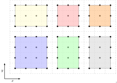
Figure 1: Example of a ParFlow mesh with $N_{x}=10$ and $N_{y}=7$. We take $N_{z}=1$ to create a two dimensional mesh, thus the value $P_{z}=1$ is implicit. The number of processes is $P_{x}=3$, $P_{y}=2$, $P=6$. Each shaded box is a subgrid, whose color symbolizes its assignment to a specific process.

It becomes clear from this logic that ParFlow’s computational mesh is distributed in parallel by assigning each of its subgrids to exactly one process via the rule (7). This order of subgrids and processes is called lexicographic.

Following the parallel distribution of the mesh, vectors and matrices in ParFlow are decomposed into subvectors and submatrices. There is a one-to-one correspondence between the subvectors/submatrices and the subgrids composing the mesh. Consequently, they are inherently distributed in parallel via the same rule (7).

2.2 Parallel exchange of information

In each time step of a simulation, a subset of degrees of freedom (dof) close to the boundary of a process’ subgrid couples to dofs lying on a foreign process (subgrid) to compute an update to its values. In ParFlow, such a subset is denoted the “dependent region.” The dependent region is derived from the stencil, a term which refers to the computational pattern determined by the numerical ansatz chosen for discretization.

Given a stencil, ParFlow automatically determines the dependent region. For each subgrid $S$, special routines loop over all subgrids in the mesh and check which of those are direct neighbors of $S$ with respect to the processes’ partition. With the data provided by the dependent region, ParFlow is able to determine the source and destination (i.e., sender and receiver) processes and the dofs relevant to the MPI messages required to perform vector and matrix updates. We will refer to this information as the MPI envelope. ParFlow implements data exchange between two neighboring subgrids via the use of a ghost layer, that is, an additional strip of artificial dof along the edges of each subgrid. Hence, data transfered via MPI messages is read from a subgrid of the sender and written into the ghost layer of the receiver. The extent of the ghost layer, i.e., the size of the strip in units of dof, is also defined by the stencil.

The lexicographic ordering principle of the subgrids has a significant impact on how the information in the MPI envelope is computed. Each subgrid $S$, as a data structure, stores its triple $(p_{x},p_{y},p_{z})$. As a consequence, the processes owning the neighbor subgrids to $S$ are located with simple arithmetic. For example, the top neighbor of $S$ is owned by the process $P_{\mathrm{own}}(p_{x},p_{y},p_{z}+1)$. The fact that there is exactly one subgrid per process implies that the process number provides sufficient information to uniquely identify the sender and receiver of MPI messages. One downside of this principle is that the number of processes determines the size of the subgrids. Essentially, using few processes requires to use a few large subgrids, while using many processes makes the subgrids fairly small. Furthermore, imagining to allow for multiple subgrids per process, the lexicographic ordering will place them in a row along the $x$-axis, leading to an elongated and thin shape of a process’ domain that has a large surface-to-volume ratio, and thus prompts a larger than optimal message size.

To organize the storage of subgrids, each process holds two arrays of type subgrid that we will denote by allsubs and locsubs, respectively. The first one stores pointers to the metadata (such as coordinates in the process grid, position and resolution) of all subgrids in the grid, and the second one stores this information only for the subgrids owned by the process (which is always one in the upstream version). Hence, the mesh metadata is replicated in every process inside of allsubs, which leads to a memory usage proportional to $P$ on every process. In practice, this disallows runs with more than 32k processes.

3 Enhancing scalability and speed of ParFlow

For large scale computations it is imperative that the mesh storage is strictly distributed. With the exception of a minimally thin ghost layer on every process’ partition boundary, any data related to the structure of the process-local mesh should be stored on this process alone. As pointed out in the previous section, such mesh storage is not implemented in ParFlow’s upstream version. This affects the runtime as well as the total memory usage: We identified loops proportional to the total number of processes $P$ in the grid allocation phase and during the determination of the dependent region that consume roughly 40 minutes on 32k processes (and would need 1h and 20 minutes on 64k processes, and so forth). Our proposed solution to enable scalability to $\mathcal{O}(10^{5})$ processes and more reads as follows.

1. Implement a strictly distributed storage of ParFlow’s computational mesh.

2. Replace loops proportional to the total number of processes with constant-size loops.

3. Allow ParFlow to use multiple subgrids per process.

The first two items are essential to enhance the scalability of the code. We aim to proceed in a minimally invasive way, reusing most of ParFlow’s mesh data structures. This principle may be called reinterpret instead of rewrite. Of course, establishing an optimized non-lexicographic and distributed mesh layout is a fairly heavy task, which is why we delegate it to a special-purpose software library described below. This removes much of the burden from the first item and lets us concentrate on the second, which requires to audit and modify the code’s accesses to mesh data. The third item serves to decouple the number of subgrids allocated from $P$, which adds to the flexibility in the setup of simulations.

Let us now describe the tools and algorithmic changes employed to realize these ideas.

3.1 The software library p4est

Tree based parallel adaptive mesh refinement (AMR) refers to methods in which the information about the size and position of mesh elements is maintained within an octree data structure whose storage is distributed across a parallel computer. An octree is basically a 1:8 (3D; 1:4 in 2D) tree structure that can be associated with a recursive refinement scheme where a cube (square) is subdivided into eight (four) half-size child cubes (squares). The leaves of the tree either represent the elements of the computational mesh directly, or can be used to hold other atomic data structures (for example one subgrid each). We will refer to the leaves of an octree/quadtree as quadrants.

The canonical domain associated with an octree is a cube (a square in 2D). When the shape of the domain is more complex, or when it is a rectangle or brick with an aspect ratio far from unity (as is the case for most regional subsurface simulations), it may be advantageous to consider a union of octrees, conveniently called a forest.

The software library p4est [5, 15] provides efficient algorithms that implement a self-consistent set of parallel AMR operations. This library creates and modifies a forest-of-octrees refinement structure whose storage is distributed using MPI parallelism. In p4est a space filling curve (SFC) determines an ordering of the quadrants that permits fast dynamic re-adaptation and repartitioning; see Figure 2. A p4est brick structure corresponds to the case in which a forest consists of multiple tree roots that are arranged to represent a rectangular Cartesian mesh.

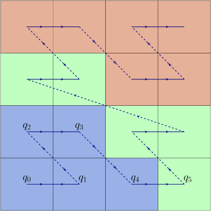
Figure 2: The space filling curve (SFC; zig-zag line) determines an ordering of the 16 quadrants $q_{i}$ obtained by a two-fold subdivision of a square. In this example we use the SFC to partition the quadrants between three processes (color coded). We use dashed lines when two elements that are adjacent in the SFC ordering are not direct face neighbors in the domain. Since most diagonal lines connect quadrants that are still indirectly face-adjacent, the process domains are localized, which makes their surface-to-volume ratio less than that of the elongated strip domains produced by a lexicographic ordering. In fact, it is known that with this SFC each process’ subdomain has at most two disconnected pieces [4].

Even when using a uniform refinement and leaving the potential for adaptivity unused, as we do in the present work, the space filling curve paradigm is beneficial since it allows to drop the restriction (2): The total number of processes does not need to match the number of patches used to split the computational mesh. Furthermore, using an SFC as opposed to a lexicographic ordering makes each process’ domain more local and approximately sphere-shaped, which reduces the communication volume on average.

3.2 Rearranging the mesh layout

The space filling curve mentioned above provides a suitable encoding to implement a strictly distributed mesh storage. Computation of parallel neighborhood relations between processes is part of the p4est algorithm bundle and encoded in the p4est ghost structure. Mesh generation, distribution and computation of parallel neighborhood relations are scalable operations in p4est, in the sense that they have demonstrated to execute efficiently on parallel machines with up to 458k processes [15].

Delegating the mesh management from ParFlow to p4est by identifying each p4est quadrant with a ParFlow subgrid allows us to inherit the scalability of p4est with relatively few changes to the ParFlow code. In particular, the following features are achievable.

1. ParFlow’s mesh storage can be trimmed down to reference only the process-local subgrid(s) and their direct parallel neighbors. As a consequence, the memory occupied by mesh storage no longer grows with $P$, and loops over subgrids take far less time.

2. The rule of fixing one subgrid per process can be relaxed. This is due to the fact that p4est has no constraints on the number of quadrants assigned to a process.

3. The computation of ParFlow’s dependent region is simplified by querying neighbor data available through the p4est ghost structure.

The main challenges arising while implementing the identification of a subgrid with a quadrant are the following.

1. Parallel neighborhood relations between processes are only known to p4est. Such information must be correctly passed on to the numerical code in ParFlow.

2. The lexicographic ordering of the subgrids will be replaced by the ordering established by p4est via the space filling curve. This means we must modify the message passing code to compute correct neighbor process indices.

3. We should add support for configurations in which a process owns multiple subgrids. This will enlarge the range of parallel configurations available and enable the option to execute the code on small size machines without necessarily reducing the number of subgrids employed. Additionally, we prepare the code for a subsequent implementation of dynamic mesh adaptation, which operates by changing the number of subgrids owned by a process at runtime.

The remainder of this section is dedicated to describe how to generate the ParFlow mesh using p4est. Essentially, we create a forest of octrees with a specifically computed number of process-local quadrants and then attach a suitably sized subgrid to each of them. Subsequently, we discuss how to obtain information on the parallel mesh layout from the p4est ghost interface.

The concept of a fixed number of processes per coordinate direction is not present in p4est. Only the total number of processes is required to compute the process partition by exploiting the properties of the space filling curve. Hence, we do not make use of the values of $P_{t}$, $t\in\{x,y,z\}$, specified by the user. Instead, we add three variables to the tcl reference script that provide values for $m_{t}$, the desired numbers of points in a subgrid along the $t$ coordinate directions. Then, we rearrange the arithmetic of (3) to compute $P_{t}$ and $l_{t}$ as derived variables satisfying

$$N_{t}=m_{t}\cdot P_{t}+l_{t},\quad P_{t}\in\mathbb{N},\quad l_{t}\in\{0,\ldots,m_{t}-1\}.$$ (8)

This construction only interprets $P_{t}$ as the number of subgrids in the $t$ direction (while the upstream version of ParFlow configures it so).

We must create a p4est object with $K:=P_{x}\times P_{y}\times P_{z}$ total quadrants. To do so, we find the smallest box containing $P_{t}$ quadrants in the $t$ direction and then refine it accordingly. Let $k_{0}$ and $g$ be defined as

$$k_{0}:=\max_{k\in\mathbb{N}}\left\{2^{k}\mid\gcd(P_{x},P_{y},P_{z})\right\},\qquad g:=2^{k_{0}}.$$ (9)

Thus, $g$ is the biggest power of two dividing the greatest common divisor of $P_{x}$, $P_{y}$ and $P_{z}$. Then, a p4est brick with dimensions

$$P_{x}/g,\quad P_{y}/g,\quad P_{z}/g,$$ (10)

and refined $k_{0}$ times will have exactly $K$ quadrants. A brick mesh resulting from applying these rules is shown in Figure 3.

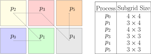
Figure 3: Left, example of a p4est brick distributed among 6 processes. Its dimensions are obtained by (10) after using $N_{x}=10$, $N_{y}=7$, $N_{z}=1$ and $m_{x}=m_{y}=3$, $m_{z}=1$ as input values in formula (8). Right, the size of the subgrids attached to each quadrant according to formula (6).

3.3 Attaching subgrids of correct size

The subgrids must be a partition of the domain in the sense that their interiors are pairwise disjoint and the union of all of them cover the grid defined by the user. These conditions impose restrictions on the choice of the parameters $N_{t}$ and $m_{t}$. Specifically, for each $t\in\{x,y,z\}$ we must require

$$\sum_{p_{t}=0}^{P_{t}-1}q(p_{t})=N_{t},$$ (11)

in order to satisfy (8). Recall that $q(p_{t})$ is defined in (6) as the length in grid points of the $p_{t}$’th subgrid along direction $t$. Condition (11) is checked prior the grid allocation phase, and in case of failure quits the program with a suitable error message specifying the pair of parameters that violated it.

We inspect the bottom left corner of each of the quadrants in the p4est brick, which by construction are only those that are local to the process, to choose the proper size of the subgrid that should be attached to it. In the native p4est format, each of these corners is encoded by three 32 bit integers that we scale with the quadrant multiplier $g$ from (9). This translates it into integer coordinates that match the enumeration $p_{t}\in\{0,\ldots P_{t}-1\}$ and are consistent with the rule (6). Thus, we can use these numbers to determine the position and dimensions of the ParFlow subgrid metadata structure that we allocate and attach to each quadrant.

3.4 Querying the ghost layer

We utilize the ghost interface of p4est to obtain the parallel neighborhood information required. Specifically, the ghost data structure provides an array of off-process quadrants that are direct face neighbors to the local partition; we call these ghost quadrants (see Figure 4). We should then populate these quadrants with suitable subgrid metadata that we use to track their identification on their respective owner processes. The p4est ghost object provides the necessary information to do this, including the lower left corner of each ghost quadrant. In fact, we can use the enumeration $p_{t}\in\{0,\ldots P_{t}-1\}$ that serves as input to equation (6) to compute the dimensions of both the local and ghost subgrids. This is most easily done by extending the loop over the p4est brick quadrants described above such that it also visits the ghost quadrants.

While we retain the interpretation of the subgrids array of the upstream version, storing pointers to the process-local subgrids, we remove almost all storage in the array allsubs: The modified version stores pointers to local and ghost subgrids in it, which are roughly a $1/P$ fraction of the total number of subgrids, and avoids allocation of even the metadata of all other, locally irrelevant subgrids that would be of order $P$. The advantage of this method is that most of the ParFlow code does not need to be changed: When it loops over the allsubs array, the loops will be radically shortened, but the relevant logic stays the same. This is the one most significant change to enable scalability to the full size of the Juqueen supercomputer (we describe these demonstrations in Section 4 below).

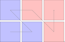
(a)

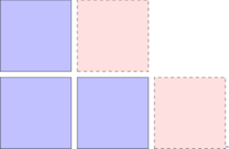
(b)

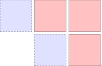
(c)

Figure 4: (a) A p4est brick with six quadrants (identified with one subgrid each) distributed among two processes (color coded). In (b) and (c) we show the view of the brick from processes zero and one, respectively. The solid boxes represent process-local quadrants, for which we allocate mesh metadata and dof storage. The dashed boxes represent quadrants in the ghost layer. For the ghost quadrants we allocate mesh metadata but no dof storage. Just as the local quadrants, the ghost quadrants are traversed in the order of the space filling curve (gray).

3.5 Further enhancements

We have edited ParFlow’s code for reading configuration files. If p4est is compiled in, we activate the according code at runtime depending on the value of a new configuration variable. Hence, even if compiled with p4est, a user has the flexibility to still use the upstream version of ParFlow on a run-by-run basis.

Additionally, we have written an alternative routine to access and distribute the information from the user-written configuration file. As before, the file is read from disk by one process and sent to all other processes, We have updated the details of this procedure, since we noticed that for high process counts (greater equal 65,536) the routine distributed incorrect data due to an integer overflow, causing the program to crash during the setup phase. The modified version delegates this task to the MPI_Bcast routine, which works reliably and fast on the usual data size of a few kilobytes.

While running numerical tests, we also encountered some memory issues. Essentially, memory allocation in ParFlow was increasing exponentially with the number of processes. With the help of the profiling tool Scalasca [9], we located the source of the problem in the preconditioner. Preconditioners in ParFlow are managed by the external dependency hypre [36], which is generally known for its scalability. Since the bug had already been resolved by the hypre community, an update to the latest version was sufficient to cure the issue.

4 Performance evaluation

In this section we evaluate the parallel performance of the modified version of ParFlow. We follow the concepts of strong and weak scaling studies. In a strong scaling analysis, a fixed problem is solved on an increasing number of processing cores and the speedup in runtime is reported. In a weak scaling study, we increase the problem size and the number of cores simultaneously such that the work and problem size per core remain the same. Ideally, the runtime should remain constant for such a study.

Weak and strong scaling studies in this work are assessed on the massively parallel supercomputer Juqueen. Juqueen is an IBM Blue Gene/Q system with 28,672 compute nodes, each with 16 GB of memory and 16 compute cores, for a total of 458,752 cores. The machine supports four way simultaneous multi-threading, though we do not make use of this capability in our studies and always run one process per core.

For each of the experiments, we collect timing information for the entire simulation. Additionally, we report timings for different components of the simulation like the solver setup, the solver itself and p4est wrap code executed. Concerning the wrap code, we refer to additional code written to execute p4est interface functions and to retrieve information from their results and propagate it to ParFlow variables. Particularly important for our purposes are the measurements related to the solver setup: The parameters for grid allocation and the management data required for the parallel exchange of information are computed during this phase.

In the past, parallel scalability of ParFlow has been evaluated mainly using weak scaling studies; see e.g., [20, 22, 31, 8]. In order to produce unbiased comparisons with these results, which are based on past upstream versions of ParFlow, we keep one subgrid per process in most of our weak scaling studies, even though we have extended the modified version to use one or optionally more. We made use of this new feature in our strong scaling studies; see Figure 12.

4.1 Weak scaling studies

In this section we present results on the weak scalability of the modified version of ParFlow. We set up a test case in which a global nonlinear problem with integrated overland flow must be solved. The test case was published previously in [25] and consists of a 3D regular topography problem in which lateral flow is driven by slopes based on sine and cosine functions. The problem has a uniform subsurface with space discretization $\Delta x=\Delta y=1.0\leavevmode\nobreak\ \mathrm{m}$, $\Delta z=0.5\leavevmode\nobreak\ \mathrm{m}$. It is initialized with a hydrostatic pressure distribution such that the top $10.0\leavevmode\nobreak\ \mathrm{m}$ of the aquifer are initially unsaturated. By doubling the number of grid points $N_{x}$ and $N_{y}$, the horizontal extent of the computational grid is increased by a factor of four per scaling step. The number of grid points in the vertical direction $N_{z}$ remains constant per scaling step. The unit problem has dimensions $N_{x}=N_{y}=50$ and $N_{z}=40$, meaning that the problem size per process is fixed to 100,000 grid points. The problem was simulated until time $t=10.0\leavevmode\nobreak\ \mathrm{s}$ using a uniform time step $\Delta t=1.0\leavevmode\nobreak\ \mathrm{s}$.

In order to offer a self-contained comparison with possible improvements in the ParFlow model platform, we conduct the weak scaling study twice, once with the upstream version of ParFlow and then with the modified version with p4est enabled. In the first case, we see that the total runtime grows with the number of processes. As can be seen in Figure 5, the solver setup routine is responsible for this behavior. Its suboptimal scaling was already reported in [22], which is in line with us noticing several loops over the all-subgrids array in this part of the code, which make the runtime effectively proportional to the total number of processes.

In the experiments we were not able to run the upstream code for 65,536 processes or more, which we attribute to a separate issue in the routine that reads user input from the configuration reference script, as we detail in Section 3.5.

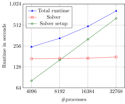
Figure 5: Weak scaling timing results for the upstream version of ParFlow. The total runtime grows with the number processes. Breaking it down into solver setup and solver execution shows that the former is responsible for the increase of the total runtime. The solver setup time grows from 81 to 639 seconds, which is perfectly proportional to the 8x increase in problem size.

Repeating the exercise with the modified version of ParFlow dramatically improves the weak scaling behavior of the solver setup; see Figures 6 and 7. With p4est enabled, we replace all loops over the total number of processes with loops of constant length. This drops the setup time from over ten minutes at 32k processes to under two seconds (by a factor of over 300). Additionally, our patch to the routine that reads the user’s configuration allows us to use as many as 262,144 processes for this study with nearly optimal, flat weak scaling. Our implementation of a strictly distributed storage of ParFlow’s mesh also leads to a reduction in memory usage at large scale; see Figure 8. This is significant for computers like Juqueen, which may only offer about two hundred megabytes if the executable is large, especially in combination with multi-threading.

We also made use of this scaling study to evaluate the relative cost of using p4est as new mesh backend by measuring the overall timing of p4est related functions introduced in in ParFlow. Our results are displayed in Figure 9.

Additionally, we employed this test case to estimate the performance of the code in terms of the floating point operations per second (FLOP/s) and compare them to the theoretical peak of the Juqueen machine. Measurements were obtained by instrumenting the code with the Scalasca profiler, which gives access to the hardware counters from the Performance Application Interface (PAPI) [32]. In particular, the number of floating point operations from a whole run have been collected and the FLOP/s estimated as a derived metric using the CUBE browser [35]. We display our results in Table 1.

	FLOP/s
# Processes	Upstream	Modified
$256$	$1.223\times 10^{8}$	$1.226\times 10^{8}$
$1024$	$1.192\times 10^{8}$	$1.194\times 10^{8}$
$4096$	$1.167\times 10^{8}$	$1.169\times 10^{8}$

Table 1: Floating point operations per second (FLOP/s) for the solver component of the upstream and modified version of ParFlow, respectively. The numbers are identical up to two significant digits. Both versions of ParFlow use roughly $3.6\%$ of the theoretical peak performance that we expect to get from a single Juqueen process, which amounts to $3.2\times 10^{9}$ FLOP/s.

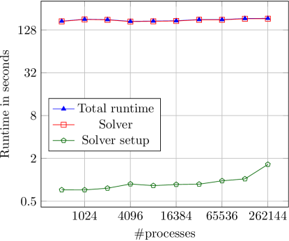
Figure 6: Weak scaling timing results of the modified version of ParFlow. The total and solver runtimes are nearly identical. In comparison to Figure 5, the solver setup executes in negligible time, ranging between $0.72$ and $1.64$ seconds.

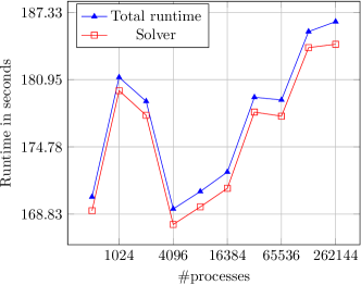
(a)

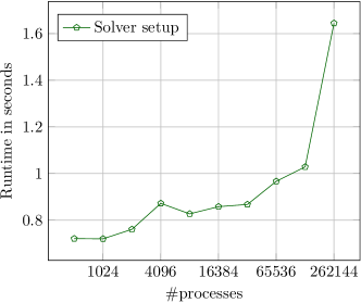
(b)

Figure 7: Split of weak scaling timing results from Figure 6. In (a) we display the total and solver runtimes that vary little in relative terms. In (b) we see that the solver setup time of the modified version of ParFlow stays under two seconds wallclock time.

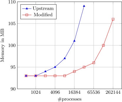
Figure 8: Weak scaling memory usage for the upstream and modified versions of ParFlow, respectively. We record the maximum heap allocation per process and plot the maximum of this quantity over all processes.

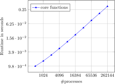
(a)

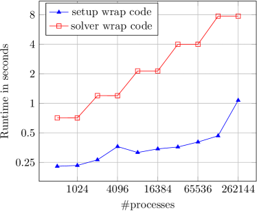
(b)

Figure 9: Top: overall timing for p4est toplevel functions used in the code. The absolute runtimes are well below one second. Bottom: We show timing results for the wrap code executed when p4est is enabled. We measure solver and setup related routines independently. Compared with the total solver time (see previous Figures), the wrap code amounts to a fraction of about 7% at most.

4.2 Strong scaling studies

In this section, we report our results on the strong scalability of the modified version of ParFlow. The test case is the same as in the previous section, with the exception of fixing $N_{x}$ and $N_{y}$ while trying a range of process counts. We divide the results of this study into two categories, depending on whether we allow for multiple subgrids per process or not.

We start with one subgrid per process. In order to keep the problem size fixed when adding more processes, we adjust the subgrid dimensions properly, i.e., by decreasing the subgrid sizes in the same proportion as the number of processes increases. We run three scaling studies, the smallest of which uses a configuration with roughly 671 million grid points. In each subsequent study we increase the problem size by a factor of four. Hence, the largest problem has around 10.7 billion grid points. In order to use the full Juqueen system under our self-imposed restriction of keeping one subgrid per process, while still obtaining runtimes comparable to the previous scaling studies, we tweak the subgrid dimensions and number of processes requested in such a way that the resulting problem size is as close as possible to 10.7 billion. Table 2 presents a summary of the main parameters defining these scaling studies; Figures 10 and 11 contain our runtime results.

	Subgrid size	number of processes	Problem size
	$m_{x}\times m_{y}\times m_{z}$	$P\times Q\times R$	$Pm_{x}\cdot Qm_{y}\cdot Rm_{z}$
	$128\times 128\times 40$	$32\times 32\times 1$	671 088 640
	$64\times 64\times 40$	$64\times 64\times 1$	671 088 640
Study 1	$32\times 32\times 40$	$128\times 128\times 1$	671 088 640
	$16\times 16\times 40$	$256\times 256\times 1$	671 088 640
	$8\times 8\times 40$	$512\times 512\times 1$	671 088 640
	$128\times 128\times 40$	$64\times 64\times 1$	2 684 354 560
	$64\times 64\times 40$	$128\times 128\times 1$	2 684 354 560
Study 2	$32\times 32\times 40$	$256\times 256\times 1$	2 684 354 560
	$16\times 16\times 40$	$512\times 512\times 1$	2 684 354 560
	$128\times 128\times 40$	$128\times 128\times 1$	10 737 418 240
Study 3	$64\times 64\times 40$	$256\times 256\times 1$	10 737 418 240
	$32\times 32\times 40$	$512\times 512\times 1$	10 737 418 240
Full system	$18\times 32\times 40$	$896\times 512\times 1$	10 569 646 080
run

Table 2: Relevant parameters for the strong scaling study under the restriction of one subgrid per process. The problem size remains constant per scaling study by setting up the subgrid dimensions inversely proportional to the number of processes.

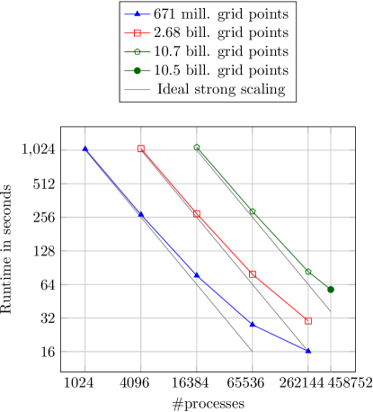
Figure 10: Strong scaling timing results of the modified version of ParFlow for different problem sizes. We plot the total runtime for each case. The solid green circle corresponds to the full size of the Juqueen system at 458,752 processes.

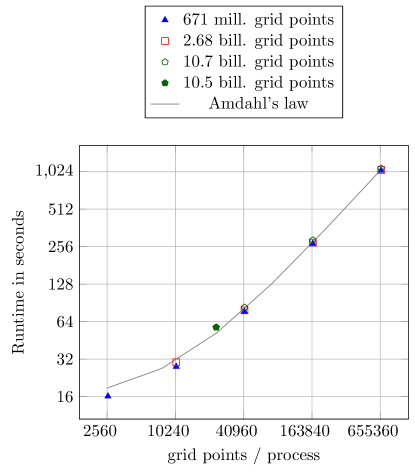
Figure 11: Strong scaling timing results of the modified version of ParFlow for different problem sizes. We plot the total runtime for each case against the number of grid points per process. The solid line shows a fit of Amdahl’s law $t=c_{1}\cdot x+c_{2}$, where $x$ denotes the number of grid points per MPI rank. The fitted parameters are $c_{1}=0.0016$ and $c_{2}=14.7$. This diagram offers another perspective on the optimality of weak scaling: We observe that measurements for simulations with the same number of grid points per process lie on top of each other in the vertical.

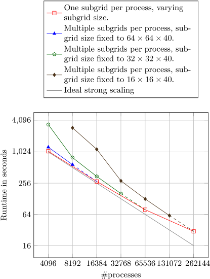
Figure 12: Strong scaling timing results of the modified version of ParFlow. We compare runs with single and multiple subgrids per process. The red line corresponds to the 2.68 billion dof single-subgrid problem (also colored red in Figure 10). Here we choose three fixed subgrid sizes (blue, green, brown). Increasing the number of processes eventually leads to a single subgrid per process, which is the case already covered in Figure 10. This limit is indicated by the final dotted segment in each graph. The largest number of subgrids per process (left end point of each graph) is four for the run represented by the blue curve, 16 for the green and 32 for the brown.

We have designed the modified version of ParFlow such that it allows for configurations in which one process may hold multiple subgrids. In practice, this option provides additional flexibility when a problem with a certain size must be run, but the number of processes available depends on external factors. Using this feature, we are able to conduct a strong scaling study without changing the subgrid size with each scaling step. To illustrate this and additionally to test that the new code supporting such configurations performs well, we take the medium size problem defined in Table 2 and execute a classical strong scaling analysis by changing only the number of processes. We do this for three different but fixed subgrid sizes. We present our results in Figure 12. We observe that increasing the number of subgrids per process incurs slightly higher simulation times but still offers nearly optimal strong scaling behavior and is thus a viable option compared to the single subgrid configuration.

5 Illustrative numerical experiment

In soil hydrology the challenge of scale is ubiquitous. Heterogeneity in soil hydraulic properties exists from the sub-centimeter to the kilometer scale related to, e.g., micro- and macro-porosity and spatially continuous soil horizons, respectively. This heterogeneity impacts the flow and transport processes in the shallow soil zone and interactions with land surface processes. Examples are groundwater recharge and leaching of nitrate and pesticides and the resulting impact on shallow aquifers. One major structural soil feature is defined by small scale preferential flow paths, developed from cracking and biota, that serve as high velocity conduits in the vertical direction. In large scale simulations, accounting simultaneously for layered soil horizons and macroporosity at the plot scale on the order to $10^{2}$ to $10^{3}$ m has been essentially impossible, because of the high spatial resolution required and the enormous size of the system of equations resulting from the boundary and initial value problem defined by the 3D Richards equation.

The improved parallel performance offered by the modified version of ParFlow motivates us to eventually target such complex simulations. In order to illustrate this, we simulate a hypothetical example configuration focused on the presence of macroporosity and layered soil horizons. The numerical experiment chosen solves an infiltration problem on a Cartesian domain. The initial water table is implemented as a constant head boundary at the bottom of the domain with a five meter unsaturated zone on top of it. The heterogeneous permeability parameter is simulated with a spatially correlated log-transformed Gaussian random field. We employ two realizations of such a field to model vertical and lateral preferential flow paths, respectively. Both random field realizations are obtained with a parallel random field generator implemented in ParFlow (the turning-bands algorithm [37]). We display an example of the outcome of such realizations and the saturation field obtained from our experiment in Figure 13.

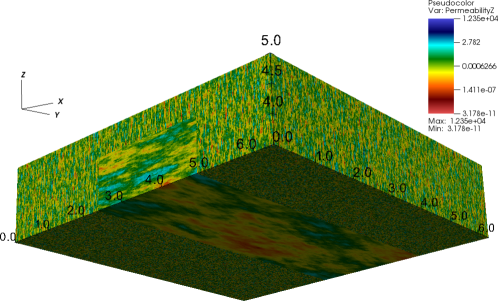
(a)

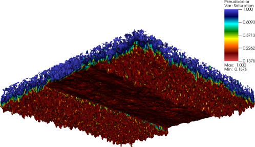
(b)

Figure 13: Picture a) shows a slice of the permeability field, generated by combining two log-transformed Gaussian random fields with standard deviations ranging over 3 orders of magnitude. In b) we display the saturation field obtained after 32,928 time steps, which correspond to 9.83 seconds simulated time. The wall clock compute time required for this simulation was around 17 hours using 16,384 MPI ranks of Juqueen.

The total compute time required was roughly 280,000 core hours. While the modified version of ParFlow can be scaled easily to use large multiples of this number, using such amounts of time must be carefully justified. At this point, it makes sense to reserve extended scientific studies for a later publication that will focus exclusively on the design and usefulness of such simulations.

6 Conclusions

The purpose of this work is to improve the parallel performance of the subsurface simulator ParFlow such it can take full advantage of the computational resources offered by the latest HPC systems. Our approach is to couple the ParFlow and p4est libraries such that the latter acts as the parallel mesh manager of the former. We achieve this with relatively small and local changes to ParFlow that constitute a reinterpretation rather than a redesign. This modified version of ParFlow offers a wider range of runnable configurations and improved performace. We report good weak and strong scaling up to 458,752 MPI ranks on the Juqueen supercomputer.

The improved performance of the modified version of ParFlow opens the possibility of bigger and more realistic simulations. For example, the code can be used to perform virtual soil column experiments to upscale hydraulic parameters related to hydraulic conductivity and the soil water retention curve. One could envision a hierarchy of experiments covering heterogeneities starting from the laboratory scale up to some 100 m. The upscaled parameters may then be used in coarser resolution models.

Considering our ehancenments, most parallel bottlenecks are gone and implementation scalability is in principle unlimited. Users should be aware that with the modified version of ParFlow, one can easily spend millions of compute hours, which demands care and sensibility in choosing the experimental setup. Nevertheless, a certain ratio of losses will be unavoidable when designing simulations at highly resolved scales due to the process of (informed) trial and error.

We also note that we did not address the algorithmic efficiency of the time stepper or the preconditioner, since the mathematics of the solver remain unchanged. Future developments in this regard will automatically inherit and benefit from the improvements in scalability reported here.

We are providing all code changes to the community, hoping for the best possible use and feedback, and will consider extending the current capabilities further when needed.

References

- [1] S. F. Ashby and R. D. Falgout, A parallel multigrid preconditioned conjugate gradient algorithm for groundwater flow simulations, Nuclear Science and Engineering, 124 (1996), pp. 145–159.
- [2] S. Balay, J. Brown, K. Buschelman, V. Eijkhout, W. D. Gropp, D. Kaushik, M. G. Knepley, L. C. McInnes, B. F. Smith, and H. Zhang, PETSc users manual, Tech. Rep. ANL-95/11 - Revision 3.3, Argonne National Laboratory, 2012.
- [3] C. Burstedde, O. Ghattas, M. Gurnis, T. Isaac, G. Stadler, T. Warburton, and L. C. Wilcox, Extreme-scale AMR, in SC10: Proceedings of the International Conference for High Performance Computing, Networking, Storage and Analysis, ACM/IEEE, 2010.
- [4] C. Burstedde, J. Holke, and T. Isaac, Bounds on the number of discontinuities of Morton-type space-filling curves. Submitted, 2017.
- [5] C. Burstedde, L. C. Wilcox, and O. Ghattas, p4est: Scalable algorithms for parallel adaptive mesh refinement on forests of octrees, SIAM Journal on Scientific Computing, 33 (2011), pp. 1103–1133.
- [6] M. Camporese, C. Paniconi, M. Putti, and S. Orlandini, Surface-subsurface flow modeling with path-based runoff routing, boundary condition-based coupling, and assimilation of multisource observation data, Water Resources Research, 46 (2010). W02512.
- [7] Y. Dai, X. Zeng, R. E. Dickinson, I. Baker, et al., The common land model, Bulletin of the American Meteorological Society, 84 (2003), p. 1013.
- [8] F. Gasper, K. Goergen, P. Shrestha, M. Sulis, J. Rihani, M. Geimer, and S. Kollet, Implementation and scaling of the fully coupled terrestrial systems modeling platform (TerrSysMP v1.0) in a massively parallel supercomputing environment – a case study on JUQUEEN (IBM Blue Gene/Q), Geoscientific Model Development, 7 (2014), pp. 2531–2543.
- [9] M. Geimer, F. Wolf, B. Wylie, E. Ábrahám, D. Becker, and B. Mohr, The scalasca performance toolset architecture, Concurrency and Computation: Practice and Experience, 22 (2010), pp. 702–719.
- [10] G. E. Hammond, P. C. Lichtner, and R. T. Mills, Evaluating the performance of parallel subsurface simulators: An illustrative example with PFLOTRAN, Water Resources Research, 50 (2014), pp. 208–228.
- [11] H. Hardelauf, M. Javaux, M. Herbst, S. Gottschalk, R. Kasteel, J. Vanderborght, and H. Vereecken, PARSWMS: A parallelized model for simulating three-dimensional water flow and solute transport in variably saturated soils, Vadose Zone Journal, 6 (2007), pp. 255–259.
- [12] R. A. Haring, M. Ohmacht, T. W. Fox, M. K. Gschwind, D. L. Satterfield, K. Sugavanam, P. W. Coteus, P. Heidelberger, M. A. Blumrich, R. W. Wisniewski, et al., The IBM Blue Gene/Q compute chip, Micro, IEEE, 32 (2012), pp. 48–60.
- [13] A. C. Hindmarsh, P. N. Brown, K. E. Grant, S. L. Lee, R. Serban, D. E. Shumaker, and C. S. Woodward, SUNDIALS: Suite of nonlinear and differential/algebraic equation solvers, ACM Transactions on Mathematical Software (TOMS), 31 (2005), pp. 363–396.
- [14] H.-T. Hwang, Y.-J. Park, E. Sudicky, and P. Forsyth, A parallel computational framework to solve flow and transport in integrated surface–subsurface hydrologic systems, Environmental Modelling & Software, 61 (2014), pp. 39–58.
- [15] T. Isaac, C. Burstedde, L. C. Wilcox, and O. Ghattas, Recursive algorithms for distributed forests of octrees, SIAM Journal on Scientific Computing, 37 (2015), pp. C497–C531.
- [16] J. E. Jones and C. S. Woodward, Newton-Krylov-multigrid solvers for large-scale, highly heterogeneous, variably saturated flow problems, Advances in Water Resources, 24 (2001), pp. 763–774.
- [17] Jülich Supercomputing Centre, JUQUEEN: IBM Blue Gene/Q supercomputer system at the Jülich Supercomputing Centre, Journal of large-scale research facilities, A1 (2015).
- [18] G. Karypis and V. Kumar, METIS – Unstructured Graph Partitioning and Sparse Matrix Ordering System, Version 2.0, 1995.
- [19] , A parallel algorithm for multilevel graph partitioning and sparse matrix ordering, Journal of Parallel and Distributed Computing, 48 (1998), pp. 71–95.
- [20] S. J. Kollet and R. M. Maxwell, Integrated surface-groundwater flow modeling: A free-surface overland flow boundary condition in a parallel groundwater flow model, Advances in Water Resources, 29 (2006), pp. 945–958.
- [21] S. J. Kollet and R. M. Maxwell, Capturing the influence of groundwater dynamics on land surface processes using an integrated, distributed watershed model, Water Resources Research, 44 (2008).
- [22] S. J. Kollet, R. M. Maxwell, C. S. Woodward, S. Smith, J. Vanderborght, H. Vereecken, and C. Simmer, Proof of concept of regional scale hydrologic simulations at hydrologic resolution utilizing massively parallel computer resources, Water Resources Research, 46 (2010), p. W04201.
- [23] M. Kuznetsov, A. Yakirevich, Y. Pachepsky, S. Sorek, and N. Weisbrod, Quasi 3d modeling of water flow in vadose zone and groundwater, Journal of Hydrology, 450–451 (2012), pp. 140–149.
- [24] X. Liu, Parallel modeling of three-dimensional variably saturated ground water flows with unstructured mesh using open source finite volume platform openfoam, Engineering Applications of Computational Fluid Mechanics, 7 (2013), pp. 223–238.
- [25] R. M. Maxwell, A terrain-following grid transform and preconditioner for parallel, large-scale, integrated hydrologic modeling, Advances in Water Resources, 53 (2013), pp. 109–117.
- [26] C. T. Miller, C. N. Dawson, M. W. Farthing, T. Y. Hou, J. Huang, C. E. Kees, C. Kelley, and H. P. Langtangen, Numerical simulation of water resources problems: Models, methods, and trends, Advances in Water Resources, 51 (2013), pp. 405–437. 35th Year Anniversary Issue.
- [27] A. Müller, M. A. Kopera, S. Marras, L. C. Wilcox, T. Isaac, and F. X. Giraldo, Strong scaling for numerical weather prediction at petascale with the atmospheric model NUMA. http://arxiv.org/abs/1511.01561, 2015.
- [28] M. Muskat, Physical principles of oil production, IHRDC, Boston, MA, Jan 1981.
- [29] OpenCFD, OpenFOAM – The Open Source CFD Toolbox – User’s Guide, OpenCFD Ltd., United Kingdom, 1.4 ed., 11 2007.
- [30] L. Orgogozo, N. Renon, C. Soulaine, F. Hénon, S. Tomer, D. Labat, O. Pokrovsky, M. Sekhar, R. Ababou, and M. Quintard, An open source massively parallel solver for richards equation: Mechanistic modelling of water fluxes at the watershed scale, Computer Physics Communications, 185 (2014), pp. 3358–3371.
- [31] D. Osei-Kuffuor, R. Maxwell, and C. Woodward, Improved numerical solvers for implicit coupling of subsurface and overland flow, Advances in Water Resources, 74 (2014), pp. 185–195.
- [32] Performance applications programming interface (PAPI). Last accessed September 7, 2017.
- [33] L. A. Richards, Capillary conduction of liquids through porous media, Physics, 1 (1931), pp. 318–33.
- [34] J. Rudi, A. C. I. Malossi, T. Isaac, G. Stadler, M. Gurnis, P. W. J. Staar, Y. Ineichen, C. Bekas, A. Curioni, and O. Ghattas, An extreme-scale implicit solver for complex pdes: highly heterogeneous flow in earth’s mantle, in Proceedings of the International Conference for High Performance Computing, Networking, Storage and Analysis, ACM, 2015, p. 5.
- [35] P. Saviankou, M. Knobloch, A. Visser, and B. Mohr, Cube v4: From performance report explorer to performance analysis tool, Procedia Computer Science, 51 (2015), pp. 1343–1352.
- [36] The Hypre Team, hypre – High Performance Preconditioners Users Manual, Center for Applied Scientific Computing, Lawrence Livermore National Laboratory, 2012. Software version 2.0.9b.
- [37] A. F. B. Tompson, R. Ababou, and L. W. Gelhar, Implementation of the three-dimensional turning bands random field generator, Water Resources Research, 25 (1989), pp. 2227–2243.
- [38] R. S. Tuminaro, M. Heroux, S. A. Hutchinson, and J. N. Shadid, Official Aztec User’s Guide, Sandia National Laboratories, sand99-8801j ed., 1999.
- [39] H. Yamamoto, K. Zhang, K. Karasaki, A. Marui, H. Uehara, and N. Nishikawa, Numerical investigation concerning the impact of CO2 geologic storage on regional groundwater flow, International Journal of Greenhouse Gas Control, 3 (2009), pp. 586–599.
- [40] K. Zhang, Y.-S. Wu, and K. Pruess, User’s guide for TOUGH2-MP a massively parallel version of the TOUGH2 code, Lawrence Berkeley National Laboratory, 2008. Report LBNL-315E.