Spherical and hyperbolic conics

1 Introduction

Most textbooks on classical geometry contain a chapter about conics. There are many well-known Euclidean, affine, and projective properties of conics. For broader modern presentations we can recommend the corresponding chapters in the textbook of Berger [2] and two recent books [1, 13] devoted exclusively to conics. For a detailed survey of the results and history before the 20th century, see the encyclopedia articles [6, 7].

At the same time, one rarely speaks about non-Euclidean conics. However, they should not be seen as something exotic. These are projective conics in the presence of a Cayley–Klein metric. In other words, a non-Euclidean conic is a pair of quadratic forms $(\Omega,S)$ on $\mathbb{R}^{3}$, where $\Omega$ (the absolute) is non-degenerate. Geometrically, a spherical conic is the intersection of the sphere with a quadratic cone; what are the metric properties of this curve with respect to the intrinsic metric of the sphere? In the Beltrami–Cayley–Klein model of the hyperbolic plane, a conic is the intersection of an affine conic with the disk standing for the plane.

Non-Euclidean conics share many properties with their Euclidean relatives. For example, the set of points on the sphere with a constant sum of distances from two given points is a spherical ellipse. The same is true in the hyperbolic plane. A reader interested in the bifocal properties of other hyperbolic conics can take a look at Theorem 6.10 or Figure 37.

In the non-Euclidean geometry we have the polarity with respect to the absolute. disk The absolute polarity exchanges distances and angles, so that for every metric theorem there is a dual one. For example, the theorem about constant sum of distances from two fixed points becomes a theorem about the envelope of lines cutting triangles of constant area from a given angle. See Figures 14 and 36.

The first systematic study of spherical conics was undertaken by Chasles. In the first part of [5] he proves dozens of metric properties of quadratic cones by elegant synthetic arguments, in the second part he interprets them as statements about spherical conics. The work of Chasles was translated from French to English and supplemented by Graves, see also [14]. A coordinate approach to spherical conics is used in [24] and [13]. Among the works on hyperbolic conics the article of Story [23] can be singled out. It uses with much success pencils of conics and the relation between $\Omega(v,w)$ and $\operatorname{dist}(v,w)$. Story’s article also contains canonical forms of equations of hyperbolic conics, see also [10, 11].

This article is to a great extent based on the works of Chasles and Story. We were unable to reproduce all of their results; this could have doubled the length of the article. An interested reader is referred to the originals.

2 Quadratic forms, conics, and pencils

2.1 The dual conic

Let $S$ be a symmetric bilinear form on a real $3$-dimensional vector space $V$. The isotropic cone of the corresponding quadratic form is the set

$$I_{S}=\{v\in V\mid S(v,v)=0\}.$$

The image of $I_{S}$ in the projective plane $P(V)$ is called a projective conic.

The form $S$ defines a linear homomorphism

$$H_{S}\colon V\to V^{*},\quad\langle H_{S}(v),w\rangle=S(v,w).$$

The symmetry of $S$ translates as the self-adjointness of $H_{S}$ with respect to the canonical pairing $\langle\cdot,\cdot\rangle$ between $V$ and $V^{*}$:

$$\langle H_{S}(v),w\rangle=\langle v,H_{S}(w)\rangle.$$

There are one-to-one correspondences between quadratic forms, symmetric bilinear forms, self-adjoint homomorphisms $V\to V^{*}$, and (complexified) isotropic cones. A conic is an equivalence class of any of the above objects under scaling. By abuse of notation we will often denote the conic by the same symbol as the symmetric bilinear form; do not forget that scaling the form does not change the conic.

The elements of $P(V^{*})$ can be interpreted as the lines in $P(V)$. Therefore a conic in $P(V)$ is called a point conic, and a conic in $P(V^{*})$ is called a line conic.

With every non-degenerate point conic one can associate a line conic. This can be done in various ways that turn out to be equivalent:

• Invert the homomorphism $H_{S}$.

• Take the image $H_{S}(I_{S})$.

• Take the set of tangents to the conic.

Lemma-Definition 2.1.

The three constructions listed above result in the same line conic, called the dual conic of $S$ and denoted by $S^{*}$.

Proof.

The first construction yields the cone

$$\{f\in V^{*}\mid\langle H_{S}^{-1}(f),f\rangle=0\},$$

and the second

$$\{H_{S}(v)\mid v\in V,\,\langle v,H_{S}(v)\rangle=0\},$$

which is clearly the same. Also, for every $v\in I_{S}$ we have

$$\ker H_{S}(v)=\{w\in v\mid S(v,w)=0\},$$

which is the plane tangent to $I_{S}$ along the line spanned by $v$. ∎

Thus for the dual conic $S^{*}$ we have

$$H_{S^{*}}=H_{S}^{-1},\quad I_{S^{*}}=H_{S}(I_{S}).$$

A degenerate point conic is a pair of lines or a double line, and a degenerate line conic is a pair of points or a double point (which means that the conic consists of all lines through these points, taken twice if the points coincide). The duality between non-degenerate point conics and line conics does not extend to degenerate ones. The best one can do is to extend the relation $H_{S}\circ H_{S^{*}}=\operatorname{Id}$ projectively, see [21, §4.D].

2.2 Euclidean vs non-Euclidean geometry

Let $\Omega$ be a non-degenerate conic in $P(V)$, hereafter called the absolute. The projective transformations from $\mathrm{PGL}(V)$ that map $\Omega$ to itself preserve the Cayley–Klein distance between the points, defined as half the logarithm of their cross-ratio with the collinear points on the absolute. They also preserve the Cayley–Klein angles between the lines, defined through their cross-ratio with the concurrent tangents to $\Omega$ (which can be interpreted as the cross-ratio of the corresponding points in $P(V^{*})$ with points on the line conic dual to $\Omega$).

For a sign-definite form $\Omega$ we obtain the elliptic geometry of $P(V)$; for an indefinite form we obtain the hyperbolic (or hyperbolic-de Sitter) geometry.

The Euclidean geometry is the geometry of a degenerate line conic that is positive definite and has rank two. Such a conic consists of lines that pass through one of two complex conjugate points. The line through these points is real and is fixed by the transformations that map the conic to itself. This designates it as the line at infinity. A degenerate line conic allows to define the Cayley–Klein angles, but not the Cayley–Klein distances. The corresponding transformation group consists of all similarity transformations.

2.3 The absolute polarity

A non-degenerate absolute $\Omega$ corresponds to a self-adjoint isomorphism $H_{\Omega}\colon V\to V^{*}$. Projectivization leads to a well-defined isomorphism between projective planes

$$[H_{\Omega}]\colon P(V)\to P(V^{*}),$$

which, together with its inverse, is called the absolute polarity. The image of a point $p\in P(V)$ is called the (absolute) polar of $p$ and denoted by $p^{\circ}$. The preimage of a line $\ell\in P(V^{*})$ is called the (absolute) pole of $\ell$ and denoted by $\ell^{\circ}$.

Equivalently, the absolute polar of a linear subspace of $V$ is its orthogonal complement with respect to $\Omega$. Here we identify the two-dimensional subspaces of $P(V)$ (that is, the lines in $P(V)$) with the points of $P(V^{*})$).

The points $[v],[w]\in P(V)$ such that $\Omega(v,w)=0$ are called conjugate with respect to $\Omega$. In other words, the polar of a point consists of all points conjugate with it.

Two lines are called conjugate if (viewed as elements of $P(V^{*})$) they are conjugate with respect to the dual quadratic form $\Omega^{-1}$. Conjugate lines contain the poles of each other.

The absolute polarity does not change when $\Omega$ is scaled, thus it is completely defined by the conic $\Omega$. The polar of a point lying on the conic is the tangent at that point. The fact that the absolute polarity preserves the incidences between the points and the lines leads to geometric constructions of poles and polars shown on Figure 1.

Figure 1: Constructing poles and polars.

2.4 The polar conic

Let, in addition to an absolute conic $\Omega$, another non-degenerate conic $S$ be given. Its dual $S^{*}$, defined in Section 2.1, is a line conic. We can use the absolute polarity to transform it to a point conic. Again, there are three equivalent descriptions of this construction.

• The homomorphism $H_{\Omega}\circ H_{S^{*}}\circ H_{\Omega}\colon V\to V^{*}$.

• The cone $H_{\Omega}^{-1}(I_{S^{*}})\subset V$.

• The poles of the tangents to the conic $S$.

Lemma-Definition 2.2.

The three constructions listed above result in the same conic, called the polar conic of $S$ and denoted by $S^{\circ}$.

Proof.

The first construction yields the set of all $v\in V$ that satisfy

$$\langle H_{\Omega}(H_{S^{*}}(H_{\Omega}(v))),v\rangle=0.$$

Since we have

$$\langle H_{\Omega}(H_{S^{*}}(H_{\Omega}(v))),v\rangle=\langle H_{S^{*}}(H_{\Omega}(v)),H_{\Omega}(v)\rangle,$$

this set is the image under $H_{\Omega}^{-1}$ of the set

$$\{f\in V^{*}\mid\langle H_{S^{*}}(f),f\rangle=0\}=I_{S^{*}}.$$

Hence the second construction is equivalent to the first.

The third construction is equivalent to the second, because the set $H_{S}(I_{S})$ consists of the tangents to the conic $S$, and the map $H_{\Omega}^{-1}$ represents the absolute polarity. ∎

As a consequence, the absolute polarity transforms conjugacy with respect to $S$ to conjugacy with respect to $S^{\circ}$.

Corollary 2.3.

A line $\ell$ is the polar of a point $p$ with respect to a conic $S$ if and only if the point $\ell^{\circ}$ is the pole of the line $p^{\circ}$ with respect to the conic $S^{\circ}$.

Proof.

The diagram

is commutative, since $H_{S^{\circ}}=H_{\Omega}\circ H_{S^{*}}\circ H_{\Omega}$ by Lemma-Definition 2.2. ∎

2.5 Pencils of conics

Since quadratic forms on a three-dimensional vector space form a vector space of dimension six, the projective conics form a five-dimensional projective space.

Definition 2.4.

A pencil of conics is a line in the projective space of conics.

A pencil spanned by the conics $S$ and $T$ consists of conics of the form $\lambda P+\mu Q$. The degeneracy condition

$$\det(\lambda P+\mu Q)=0$$

is a homogeneous polynomial of degree $3$ in $\lambda$ and $\mu$. Therefore either all or at most three conics of a pencil are degenerate.

Example 2.5 (Conics through four points).

Consider a pencil that contains two pairs of lines. If a line of one pair coincides with a line of the other pair, then this line is contained in all conics of the pencil, hence all conics are degenerate. If all four lines are distinct, then the first pair intersects the second pair in four points, and the pencil consists of the conics through these four points, see Figure 2, left. In particular, it contains a third degenerate conic made of a third pair of lines.

Example 2.6 (Double contact pencil).

Consider a pencil that contains a pair of lines $\ell_{1},\ell_{2}$ and a double line through the points $p_{1}\in\ell_{1}$ and $p_{2}\in\ell_{2}$ (assuming that neither $p_{1}$ nor $p_{2}$ is the intersection point of $\ell_{1}$ and $\ell_{2}$). Then every conic of the pencil goes through the points $p_{1}$ and $p_{2}$ and is tangent to the lines $\ell_{1}$ and $\ell_{2}$ at these points (the latter can be seen by viewing the double line as a limit of pairs of lines). See Figure 2, right.

Figure 2: Pencil of conics through four real points and a real double contact pencil.

There are pencils that involve imaginary elements, for example the pencil of conics through two pairs of complex conjugate points.

For more details, including other types of pencils with illustrations, see [1, 3.3], [2, 16.4], and [13, 7.3]

2.6 Dual pencils and confocal conics

Take a pencil $\mathcal{P}$ of line conics, that is a line in the space of conics in $P(V^{*})$. The non-degenerate conics of $\mathcal{P}$ can be dualized (see Section 2.1). This gives a family of point conics, called a dual pencil or a tangential pencil.

Example 2.7.

Let $\mathcal{P}$ be a pencil of line conics through four lines in general position. The corresponding dual pencil consists of non-degenerate point conics tangent to those lines. The degenerate members of $\mathcal{P}$ are three pairs of interection points of the four lines. Thus, in a sense, the dual pencil is spanned by the three diagonals of a complete quadrilateral. Intuitively, these diagonals are degenerate ellipses tangent to the four lines.

Example 2.8.

Let $\mathcal{P}$ be a double contact pencil. The dual pencil is also (the non-degenerate part of) a double contact pencil: since the dual conic is made of tangents, the dual of a conic tangent to $\ell$ at $p$ is a line conic “tangent to” $p$ at $\ell$. The degenerate members of this dual pencil are a pair of points (the points of contact) and a double point (the intersection point of the lines of contact).

Definition 2.9.

If a pencil of line conics contains the dual absolute, then the corresponding dual pencil is called a confocal family of conics.

The definition also makes sense in the Euclidean geometry, where the dual absolute conic is degenerate, see Section 2.2.

We define the foci of spherical and hyperbolic conics in Sections 3.3 and 5.3 and discuss confocal families in Sections 3.5 and 5.7 in more detail.

Lemma 2.10.

Confocal conics intersect orthogonally.

Proof.

This statement means that the tangents of two confocal conics at their intersection point are conjugate with respect to the absolute. Equivalently (in terms of line conics), the points of tangency of a common tangent to two conics of a pencil are conjugate with respect to any conic from this pencil, see Figure 3. But since these points are conjugate with respect to the conics to which they belong, they are so with respect to any linear combination. ∎

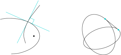
Figure 3: Confocal conics intersect orthogonally, and the dual statement.

Example 2.11.

A special case of confocal conics is the dual of the pencil spanned by the dual absolute and a double point $2p$. If $p$ does not lie on the absolute, then this is a double contact pencil spanned by the tangents from $p$ to $\Omega$ and the double polar of $p$. This pencil is made by the circles centered at $p$, which can be shown by a simple computation. (In the hyperbolic case, $p$ can be hyperbolic, de Sitter, or ideal point, see Lemma 6.3.)

2.7 Chasles’ theorems

Chasles’ article [4] contains a variety of theorems, whose proofs follow all the same principle. A pencil of conics is a line in the projective space of all conics. If in a collection of lines there are many concurrent pairs, then all lines are coplanar, and hence any two of them are concurrent. Translated to pencils of conics, this means that if in a collection of pencils many pairs share a conic, then any two of these pencils share a conic. The argument also works for dual pencils, since they correspond to lines in the space of line conics, and in particular for confocal families of conics.

The following theorem is one of those contained in [4].

Theorem 2.12 (Chasles).

Let $\{\ell_{i}\}_{i=1}^{4}$ be four tangents to a conic $A$. Denote by $p_{ij}$ the intersection point of $\ell_{i}$ and $\ell_{j}$. Assume that the points $p_{12}$ and $p_{34}$ lie on a conic $B$ confocal to $A$. Then the following holds.

1. The pairs of points $p_{13},p_{24}$ and $p_{14},p_{23}$ also lie on conics confocal to $A$.

2. The tangents at the points $p_{ij}$ to the three conics that contain pairs of points meet at the same point $q$.

3. There is a circle tangent to the lines $\ell_{i}$, and this circle is centered at $q$.

If, in the hyperbolic case, the point $q$ is ideal or de Sitter, then the role of a circle centered at $q$ is played by a horocycle or a hypercycle.

Figure 4: Chasles’ theorem.

Proof.

The idea is to dualize the picture, so that confocal conics become conics collinear with the dual absolute, see Section 2.6.

Consider two pencils of line conics: one spanned by $A^{*}$ and the dual absolute, the other made by conics through the lines $\ell_{i}$ (duals of conics tangent to these lines). The second pencil contains the conics $A^{*}$, $p_{12}+p_{34}$, $p_{13}+p_{24}$, and $p_{14}+p_{23}$ (the latter three line conics are degenerate, see the last paragraph of Section 2.1). Since the two pencils share the conic $A^{*}$, they lie in a plane in the projective space of line conics.

Consider the pencil of line conics spanned by $B^{*}$ and $p_{12}+p_{34}$. This is a double contact pencil; it contains the double point $2q$, where $q$ is the intersection point of the tangents to $B$ at $p_{12}$ and $p_{34}$. See Figure 5, where the line conics are depicted as points.

Figure 5: Proof of the Chasles theorem.

The pencil of line conics spanned by $p_{14}+p_{23}$ and $2q$ and the pencil spanned by $A^{*}$ and $\Omega^{*}$ have a conic in common. Its dual is a point conic confocal with $A$ and tangent at the points $p_{14}$ and $p_{23}$ to the lines $p_{14}q$ and $p_{23}q$. The same is true with $p_{13}+p_{24}$ in place of $p_{14}+p_{23}$, which proves the first two parts of the theorem.

For the third part, consider the pencil spanned by $\Omega^{*}$ and $2q$. It consists of circles centered at $q$ (for the hyperbolic case, see Lemma 6.3). This pencil intersects the pencil of conics through the lines $\ell_{i}$, hence there is a circle centered at $q$ tangent to those lines. ∎

The third part of the theorem is related to the following property of confocal conics: a billiard trajectory inside a conic is tangent to a confocal conic.

2.8 Projective properties

Theorems of Pascal, Brianchon, and Poncelet deal with projective properties of conics, therefore they hold for non-Euclidean conics as well as for Euclidean ones. However, in the non-Euclidean case one can obtain new theorems from known ones by modifying them as follows.

• Apply the absolute polarity to some of the elements.

• If there is one or several conics in the premises of the theorem, assume one of them to be the absolute conic.

• If there are several conics, assume two of them to be polar to each other.

Theorems below illustrate this.

Theorem 2.13.

The common perpendiculars to the pairs of opposite sides of a spherical or hyperbolic hexagon intersect in a point if and only if the hexagon is inscribed in a conic.

Proof.

The common perpendicular to two lines $\ell_{1}$ and $\ell_{2}$ is the line through the poles $\ell_{1}^{\circ}$ and $\ell_{2}^{\circ}$. A hexagon is inscribed in a conic if and only if its polar dual is circumscribed about a conic. Hence this theorem follows from the Brianchon theorem by applying the absolute polarity. ∎

Theorem 2.14.

The diagonals and the common perpendiculars to the opposite pairs of sides in an ideal hyperbolic quadrilateral meet at a point.

Proof.

The common perpendiculars are the diagonals of the polar quadrilateral, which is circumscribed about the absolute. The diagonals and the lines joining the opposite points of tangency meet at a point; this is a limit case of the Brianchon theorem. ∎

Theorem 2.15.

The set of points from which a (Euclidean or non-Euclidean) conic is seen under the right angle is also a conic.

Proof.

The tangents drawn from a point to the conic are orthogonal if and only if they harmonically separate the tangents to the absolute conic. This set of points is called the harmonic locus of the conic and the absolute. The harmonic locus of any two conics is a conic; this can be proved with the help of Chasles’ theory of $(2\textendash 2)$ correspondences, see [8, §50]. ∎

The set of points from which a curve is seen under the right angle is called the orthoptic curve. In the Euclidean case, the orthoptic curve of a conic is a circle.

Theorem 2.16.

Choose any tangent $\ell_{1}$ to a non-Euclidean conic $S$. Let $\ell_{2}$ be a tangent to $S$ perpendicular to $\ell_{1}$, let $\ell_{3}$ be a tangent to $S$ perpendicular to $\ell_{2}$ and different from $\ell_{1}$, and so on. Assume that for some $n$ we have $\ell_{n+1}=\ell_{1}$. Then the same holds for any other choice of the tangent $\ell_{1}$.

First proof.

This is the Poncelet theorem for the conic $S$ and its orthoptic conic. ∎

Second proof.

The intersection point of the lines $\ell_{1}$ and $\ell_{3}$ is the pole of $\ell_{2}$, which lies on $S^{\circ}$. Hence $\ell_{1},\ell_{3},\ell_{5},\ldots$ is a Poncelet sequence for the conic $S$ and its polar $S^{\circ}$, see Figure 6, left. By assumption, for $n$ odd it closes after $n$ steps, hence it closes after $n$ steps for any choice of $\ell_{1}$. For $n$ even, we have two sequences that close after $\frac{n}{2}$ steps. ∎

Figure 6: A non-Euclidean variation of the Poncelet theorem.

Corollary 2.17.

A spherical ellipse inscribed in a regular right-angled triangle can be rotated while staying inscribed in that triangle. See Figure 6, right.

Dually, a spherical ellipse circumscribed about a regular right-angled triangle can be rotated while staying circumscribed. See also [Theorem 10.1.11]GSO16.

3 Spherical conics

3.1 A spherical conic and its polar

Algebraically, a spherical conic is a pair of quadratic forms $(\Omega,S)$ on a $3$-dimensional vector space, with $\Omega$ positive definite. In an appropriate basis we have

$$\Omega(v,v)=x^{2}+y^{2}+z^{2}.$$

Geometrically, a spherical conic is an intersection of the unit sphere in $\mathbb{R}^{3}$ with a quadratic cone. If the cone is degenerate, then the conic consists of two great circles or of one “double” great circle. If the cone is circular, then the conic is a pair of diametrically opposite small circles. The most interesting is the case when the cone is non-degenerate and non-circular, which we always assume in the sequel.

By the principal axes theorem, there is a basis in which $\Omega$ keeps its form, while the quadratic form defining the cone becomes diagonal:

$$C=\{v\in\mathbb{R}^{3}\mid S(v,v)=0\},\quad S(v,v)=\frac{x^{2}}{a^{2}}+\frac{y^{2}}{b^{2}}-\frac{z^{2}}{c^{2}},\quad a>b.$$ (1)

The polar conic is then given by

$$C^{\circ}=\{v\in\mathbb{R}^{3}\mid S^{\circ}(v,v)=0\},\quad S^{\circ}(v,v)=a^{2}x^{2}+b^{2}y^{2}-c^{2}z^{2}.$$ (2)

Following Chasles, we call the $z$-axis the principal axis, the $x$-axis the major axis, and the $y$-axis the minor axis of $C$. The polar cone has the same principal axis, but the major and the minor axes become interchanged. The points where the axes intersect the sphere are called the centers of the conic.

3.2 Projections of a spherical conic

A spherical conic is a spatial curve of degree $4$, but from a carefully chosen point of view it takes a more recognizable shape.

Theorem 3.1.

The orthogonal projection of a spherical conic along the principal axis is an ellipse. The projection along the major axis consists of two arcs of a hyperbola, and the projection along the minor axis consists of two arcs of an ellipse. See Figure 7.

Figure 7: Orthogonal projections of a spherical conic along the axes.

Proof.

The pencil of affine quadrics spanned by $\Omega=1$ and $S=0$ contains the following three cylinders.

$$\left(\frac{1}{a^{2}}+\frac{1}{c^{2}}\right)x^{2}+\left(\frac{1}{b^{2}}+\frac{1}{c^{2}}\right)y^{2}=\frac{1}{c^{2}}$$

$$\left(\frac{1}{a^{2}}+\frac{1}{c^{2}}\right)z^{2}-\left(\frac{1}{b^{2}}-\frac{1}{a^{2}}\right)y^{2}=\frac{1}{a^{2}}$$

$$\left(\frac{1}{b^{2}}-\frac{1}{a^{2}}\right)x^{2}+\left(\frac{1}{b^{2}}+\frac{1}{c^{2}}\right)z^{2}=\frac{1}{b^{2}}$$

Each of these cylinders intersect the sphere along the conic $S$. Hence the projection of the conic along the axis of a cylinder is the part of an orthogonal section of the cylinder that lies inside the unit disk. ∎

3.3 Foci and focal lines of a spherical conic

Every quadratic cone has a circular section, a fact that was established by Descartes. Any two parallel sections (not passing through the origin) are similar.

Definition 3.2.

A cyclic plane of a quadratic cone is a plane through the origin such that every parallel plane intersects the cone in a circle. The intersection of a cyclic plane with the unit sphere is a great circle called a focal line of the spherical conic.

A non-circular cone has two cyclic planes, both passing through the major axis and symmetric to each other with respect to the plane spanned by the principal and the major axes.

Definition 3.3.

A cocyclic line of a quadratic cone is the orthogonal complement of the cyclic plane of the polar cone. The intersection of a cocyclic line with the sphere is an antipodal pair of points called a focus of the spherical conic.

A non-circular cone has two cocyclic lines, both of which lie in the plane of the principal and the major axes. Accordingly, a spherical conic has two foci.

Theorem 3.4.

The cyclic planes of the cone $C$ from (1) are given by the equation

$$\sqrt{\frac{1}{b^{2}}-\frac{1}{a^{2}}}y\pm\sqrt{\frac{1}{c^{2}}+\frac{1}{a^{2}}}z=0.$$

The cocyclic lines of the cone $C$ from (2) are spanned by the vectors

$$(\sqrt{a^{2}-b^{2}},\,0,\,\pm\sqrt{b^{2}+c^{2}}).$$

Proof.

The pencil of quadrics $S+\lambda\Omega$ contains a pair of planes

$$S-\frac{1}{a^{2}}\Omega=\left(\frac{1}{b^{2}}-\frac{1}{a^{2}}\right)y^{2}-\left(\frac{1}{c^{2}}+\frac{1}{a^{2}}\right)z^{2}.$$

Hence the restriction of $S$ to each of the planes is proportional to the restriction of $\Omega$. This implies that the sections of $C^{\circ}$ parallel to these planes are circular.

The formulas for the cocyclic lines of $C$ follow by computing the cyclic planes of $C^{\circ}$ and applying polarity. ∎

Corollary 3.5.

For every spherical conic, the intersection of its cyclic planes with the plane of the principal and minor axes are the asymptotes of the hyperbola that contains the projection of the conic to that plane. See Figure 7, left.

Let us now describe some geometric properties of the cocyclic lines.

Theorem 3.6.

Two planes through a cocyclic line of a quadratic cone are orthogonal if and only if they are conjugate with respect to the cone.

Proof.

By Corollary 2.3, orthogonality with respect to $S$ translates into orthogonality of the polars with respect to $S^{\circ}$. Polars of planes through a cocyclic line of $C$ are lines in a cyclic plane of $C^{\circ}$. In this plane, the forms $S^{\circ}$ and $\Omega$ are proportional to each other; in particular, two lines are orthogonal with respect to $S$ if and only if they are orthogonal with respect to $\Omega$. ∎

\begin{picture}(7987.0,3673.0)(-4577.0,-975.0)\end{picture}

Figure 8: Planes parallel to cyclic planes intersect a cone along a circle. Planes through cocyclic lines are orthogonal if and only if they are conjugate.

Corollary 3.7.

The plane tangent to $\mathbb{S}^{2}$ at a focus $F$ of a spherical conic intersects the corresponding cone along an ellipse with a focus at $F$.

Proof.

Let $\pi$ be the tangent plane to $\mathbb{S}^{2}$ at $F$. Orthogonal planes through a focal line intersect $\pi$ along orthogonal lines. Thus by the previous theorem two lines in $\pi$ that pass through $F$ are orthogonal if and only if they are conjugate with respect to the ellipse $C\cap\pi$. This property characterizes the foci of a Euclidean ellipse, see [2, §17.2.1.6] ∎

The following lemma about circular sections will be particularly useful.

Lemma 3.8.

Every sphere passing through a circular section of a quadratic cone intersects it along another circle. Conversely, any two non-parallel circular sections of a quadratic cone are contained in a sphere.

Proof.

Consider the inversion with center at the apex of the cone that sends the sphere to itself. Since the inversion also fixes the cone, it exchanges the two components of the intersection. Therefore, if one component is a circle, so is the other.

For the second part, find an inversion that sends one circular section to the other. Then an invariant sphere passing through one of the circles passes also through the other. ∎

In the limit, as one of the circular sections tends to a point, we obtain the following.

Corollary 3.9.

Every sphere tangent to a cyclic plane at the apex of the cone intersects the cone in a circle.

3.4 Directors and directrices

Definition 3.10.

A line through the origin conjugate with respect to a quadratic cone to one of its cyclic planes is called a director line of the cone. The intersection of a director line with the sphere (that is, the pair of poles of a focal line with respect to the conic) is called a director of a spherical conic.

In other words, the director lines are formed by the centers of circular sections of the cone.

Definition 3.11.

A plane through the origin conjugate with respect to a quadratic cone to one of its cocyclic lines is called a directrix plane of the cone. The intersection of a directrix plane with the sphere (that is, the polar of a focus with respect to a conic) is called a directrix of a spherical conic.

By Corollary 2.3, the directrix of a conic is polar to the director point of the polar conic.

From the formulas of Theorem 3.4 it follows that the director lines of the cone $C$ are spanned by the vectors

$$\left(0,\,b\sqrt{1-\frac{b^{2}}{a^{2}}},\,\pm c\sqrt{1+\frac{c^{2}}{b^{2}}}\right),$$

and its directrix planes have the equations

$$\frac{\sqrt{a^{2}-b^{2}}}{a^{2}}x\pm\frac{\sqrt{b^{2}+c^{2}}}{c^{2}}z=0.$$

3.5 Families of spherical conics

A spherical conic $S$ intersects the absolute conic $\Omega$ in four imaginary points that form two complex conjugate pairs (the points are distinct since we assumed the cone to be non-circular).

Theorem 3.12.

The focal lines of a spherical conic are the lines through the complex conjugate pairs of intersection points of the conic with the absolute.

Proof.

This follows from the computation in the proof of Theorem 3.4. But here is an alternative coordinate-free argument. A cyclic plane of a quadratic cone is a plane on which the restrictions of $\Omega$ and $S$ are proportional. In particular, $\Omega$ and $S$ must vanish at the same time. This implies that a cyclic plane is spanned by two common (imaginary) isotropic lines of $\Omega$ and $S$. Projectively, a cyclic line is a line through two intersection points of $\Omega$ and $S$. For this line to be real, the points must be complex conjugate. ∎

As a consequence, conics that share the focal lines with the conic $S$ form a pencil of conics through four imaginary points, spanned by $\Omega$ and $S$. In coordinates, this pencil is given by the equations

$$\left(\frac{1}{a^{2}}-\lambda\right)x^{2}+\left(\frac{1}{b^{2}}-\lambda\right)y^{2}-\left(\frac{1}{c^{2}}+\lambda\right)z^{2}=0.$$ (3)

One can visualize the conics with common focal lines as follows.

Theorem 3.13.

Every hyperboloid asymptotic to the cone over a spherical conic $S$ intersects the sphere along a spherical conic that shares the focal lines with $S$.

Proof.

A hyperboloid asymptotic to the cone over $S$ is given by an equation of the form

$$\frac{x^{2}}{a^{2}}+\frac{y^{2}}{b^{2}}-\frac{z^{2}}{c^{2}}=\lambda.$$

By taking a linear combination with the equation of the sphere, we see that the hyperboloid intersects the sphere along the same curve as the cone (3). ∎

By definition of the foci and directrices, we have the following.

Theorem 3.14.

A focus of a spherical conic is the intersection point of two (complex conjugate) common tangents to the conic and the absolute. The corresponding directrix is the line through the points where these tangents touch the conic.

That is, conics confocal with $S$ form a dual pencil to the one spanned by $S^{\circ}$ and $\Omega$ and are given by the equations

$$\frac{x^{2}}{a^{2}-\lambda}+\frac{y^{2}}{b^{2}-\lambda}-\frac{z^{2}}{c^{2}+\lambda}=0,\quad\lambda\in(-1,b^{2})\cap(b^{2},a^{2}).$$ (4)

Corollary 3.15.

Conics that share a focus and a corresponding directrix form a double contact pencil (determined by two complex conjugate points on two complex conjugate lines).

4 Theorems about spherical conics

4.1 Ivory’s lemma

On the turn of the 18th century, Laplace and Ivory [15] computed the gravitational field created by a solid homogeneous ellipsoid. Ivory’s solution was immediately and widely recognized for its elegance, see [27][§§1141, 1146]. Chasles [4] further simplified Ivory’s argument; it is under this form that it is presented nowadays, see e. g. [12, Lecture 30]. In particular, Chasles stated explicitely what is now called the Ivory lemma.

Ivory’s lemma is a statement about confocal conics and quadrics. Its original version deals with confocal quadrics in the Euclidean $3$-space, but it holds in any dimension with respect to any Cayley–Klein metric, see [22].

In this section we prove Ivory’s lemma on the $2$-sphere.

Theorem 4.1 (Ivory’s lemma).

The diagonals in a quadrilateral formed by four confocal spherical conics have equal lengths.

Figure 9 illustrates Ivory’s lemma in the Euclidean plane. It can also be interpreted as a distorted view of confocal spherical conics.

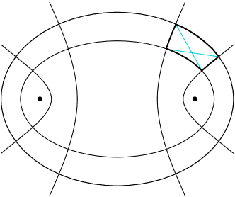
Figure 9: Ivory’s lemma.

Take our quadratic cone $C$ and a cone $C_{\lambda}$ given by equation (4) with $-1<\lambda<b^{2}$, which ensures that the corresponding confocal conics don’t intersect. Consider a linear map $\mathbb{R}^{3}\to\mathbb{R}^{3}$ given by the diagonal matrix

$$F_{\lambda}=\operatorname{diag}\left(\frac{\sqrt{a^{2}-\lambda}}{a},\frac{\sqrt{b^{2}-\lambda}}{b},\frac{\sqrt{c^{2}+\lambda}}{c}\right).$$

Lemma 4.2.

The map $F_{\lambda}$ sends the spherical conic $S=C\cap\mathbb{S}^{2}$ to the conic $S_{\lambda}=C_{\lambda}\cap\mathbb{S}^{2}$. Besides, if a point $v\in S$ belongs to a conic $S_{\mu}$, then $F_{\lambda}(v)$ also belongs to $S_{\mu}$.

Proof.

Denote $A=\operatorname{diag}(a^{2},b^{2},-c^{2})$. Then $C$, $C_{\lambda}$, and $C_{\mu}$ are the isotropic cones of the matrices

$$S=A^{-1},\quad S_{\lambda}=(A-\lambda\operatorname{Id})^{-1},\quad S_{\mu}=(A-\mu\operatorname{Id})^{-1},$$

respectively. By definition of $F_{\lambda}$ we have

$$F_{\lambda}^{2}=(A-\lambda\operatorname{Id})A^{-1},$$

which immediately implies $F_{\lambda}(C)=C_{\lambda}$. Further, observe that

$$\|F_{\lambda}(v)\|^{2}=v^{\top}(A-\lambda\operatorname{Id})A^{-1}v=v^{\top}v-\lambda v^{\top}A^{-1}v=\|v\|^{2}-\lambda v^{\top}Sv=1,$$

provided that $v\in\mathbb{S}^{2}\cap C$. Hence, $v\in S$ implies $v\in S_{\lambda}$.

We also have

$$F_{\lambda}S_{\mu}F_{\lambda}=A^{-1}(A-\lambda\operatorname{Id})(A-\mu\operatorname{Id})^{-1}=(A-\mu\Omega)^{-1}-\lambda A^{-1}(A-\mu\operatorname{Id})^{-1}\\ =(A-\mu\operatorname{Id})^{-1}-\frac{\lambda}{\mu}((A-\mu\operatorname{Id})^{-1}-A^{-1})=\frac{\lambda}{\mu}A^{-1}+\left(1-\frac{\lambda}{\mu}\right)(A-\mu\operatorname{Id})^{-1}.$$

In other words,

$$F_{\lambda}(v)^{\top}S_{\mu}F_{\lambda}(v)=\frac{\lambda}{\mu}v^{\top}Sv+\left(1-\frac{\lambda}{\mu}\right)v^{\top}S_{\mu}v,$$

so that $v\in C\cap C_{\mu}$ implies $v\in C_{\mu}$. ∎

Proof of Theorem 4.1.

Let $S$, $S_{\lambda}$, $S_{\mu_{1}}$, and $S_{\mu_{2}}$ be confocal conics such that $S$ and $S_{\lambda}$ are disjoint, and $S_{\mu_{1}}$, $S_{\mu_{2}}$ intersect them. Let $v_{i}\in S\cap S_{\mu_{i}}$ and $w_{i}\in S_{\lambda}\cap S_{\mu_{i}}$, $i=1,2$. We want to show that $\operatorname{dist}(v_{1},w_{2})=\operatorname{dist}(v_{2},w_{1})$.

By Lemma 4.2, $w_{i}=F_{\lambda}(v_{i})$. Since the matrix $F_{\lambda}$ is diagonal, we have

$$v_{1}^{\top}w_{2}=v_{1}^{\top}F_{\lambda}v_{2}=w_{1}^{\top}v_{2},$$

which implies the desired equality of diagonals. ∎

Remark 4.3.

The most general form of the Ivory lemma was discovered by Blaschke [3]: it holds in the coordinate nets of Stäckel metrics (in dimension $2$ known as Liouville nets). Conversely, if a coordinate net on a Riemannian manifold has the equal diagonals property, then it is a Stäckel net. The argument uses integrals of the geodesic flow and is inspired by Jacobi’s ideas from his study of geodesics on ellipsoids. For a modern exposition, see [25, 16].

4.2 Bifocal properties of spherical conics

On the illustrations to the following theorems we are using the projective model of the sphere: the projection of the sphere from its center to a tangent plane. A spherical conic becomes an affine conic, all great circles (in particular, the focal lines of the conic) become straight lines. As a projection plane, it is convenient to choose a plane that is tangent at one of the centers of the conic, see Figure 10.

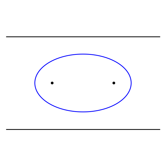
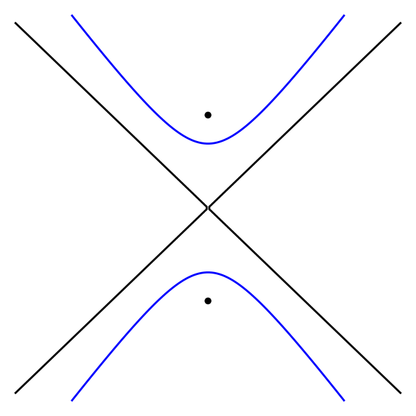
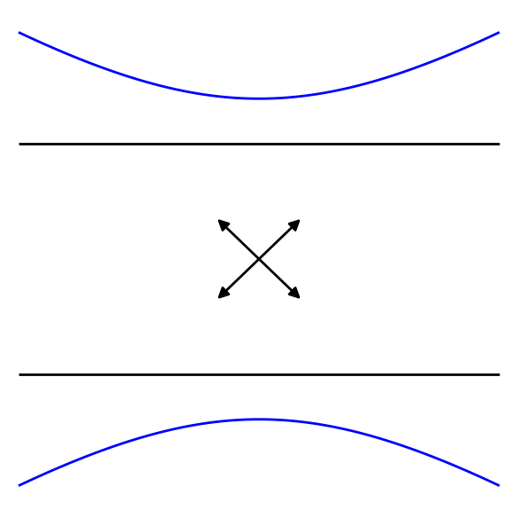
Figure 10: Projections of a spherical conic to the planes tangent to its centers.

The focal lines on Figure 10, middle, are not the asymptotes of the hyperbola; the arrows in the center of Figure 10, right, indicate the position of the foci, which belong to the line at infinity.

Each of the theorems below consists of two parts, dual to each other via the absolute polarity. Therefore we are proving only one part of each theorem. Usually this is the part that deals with the focal lines, because in the space it deals with circles and spheres and can be proved by an elegant synthetic argument. All proofs were given by Chasles in [5].

Theorem 4.4.

1. For every tangent to a spherical conic, the point of tangency bisects the segment comprised between the focal lines.

2. The lines joining the foci of a spherical conic with a point on the conic form equal angles with the tangent at that point.

Figure 11: The bisector property.

Proof.

Interpreted in terms of the corresponding quadratic cone, the first statement becomes as follows: any plane tangent to the cone intersects the cyclic planes along the lines that make equal angles with the line of tangency.

Take two planes parallel to the cyclic planes; they intersect the cone in two non-parallel circles. By Lemma 3.8, these circular sections are contained in a sphere. A tangent plane to the cone intersects the planes of the circles in two lines tangent to the sphere, see Figure 13, left. We need to show that these lines make equal angles with the line of tangency. But any two tangents to the sphere make equal angles with the segment joining their points of tangency, and the theorem is proved. ∎

Theorem 4.4 can be viewed as a limit case of the following.

Theorem 4.5.

1. For every secant line of a spherical conic the segments comprised between the conic and the focal lines have equal lengths.

2. For every point outside of a spherical conic, the angle between a tangent through this point and the line joining the point to a focus is equal to the angle between the other tangent and the line to the other focus.

Figure 12: The generalized bisector property.

Proof.

The first statement says that every plane through two generatrices of the cone intersects the cyclic plane along two lines such that the angle between a line and a generatrix is equal to the angle between the other line and the other generatrix.

Translate the cyclic planes so that they intersect the cone along two circles. By Lemma 3.8 these two circles are contained in a sphere. The generatrices and the intersection lines of the secant plane with the planes spanned by the circles form a planar quadrilateral inscribed in the sphere, see Figure 13, right. Two opposite angles of this quadrilateral complement each other to $\pi$, which implies the theorem. ∎

Figure 13: Proofs of Theorems 4.4 and 4.5.

Theorem 4.6.

1. A tangent to a spherical conic cuts from the lune formed by the focal lines a triangle of constant area.

2. The sum of the distances from a point on a spherical conic to its foci is constant.

The first part is dual to the second, because the area of a spherical triangle is equal to its angle sum minus $\pi$. Since the angle at the vertex $E$ is constant, the statement is equivalent to the constancy of the sum of the angles at $X$ and $Y$. These angles are equal to the lengths of $F_{1}Z$ and $F_{2}Z$ in the second part of the theorem.

Figure 14: Bifocal properties: $\operatorname{Area}(\triangle EXY)=\mathrm{const}$, $F_{1}Z+F_{2}Z=\mathrm{const}$.

The second part is due to Magnus [18], who proved it by a direct computation. Two different proofs are given below: the first one uses differentiation, the second one synthetic geometry. The latter is due to Chasles and uses Theorem 4.7 below.

First proof.

When we move a line keeping it tangent to the conic, the instantaneous change in the area of the triangle is zero because, by the first part of Theorem 4.4, the point of tangency bisects the segment $XY$. Similarly, for a point moving along the conic, the derivative of the sum of its distances from the foci is zero by the second part of Theorem 4.4. ∎

Second proof.

The second part of Theorem 4.6 can be derived from the second part of Theorem 4.7 similarly to the proof that in a circumscribed quadrilateral the sums of opposite pairs of sides are equal. Take two points $A$ and $B$ on a conic such that the segments $F_{1}A$ and $F_{2}B$ intersect. By Theorem 4.7 there is a circle tangent to the lines $F_{1}A,F_{1}B,F_{2}A,F_{2}B$. Since tangent segments drawn from a point to a circle have equal lengths, we have (see Figure 15)

$$F_{1}A+F_{2}A=F_{1}K+F_{2}L=F_{1}M+F_{2}N=F_{1}B+F_{2}B.$$

Figure 15: Second proof of Theorem 4.6.

∎

Theorem 4.7.

1. Two tangents to a spherical conic intersect the focal lines in four points that are equidistant from the line through the points of tangency.

2. Four lines joining the foci of a spherical conic with two points on the conic are tangent to a circle. The center of this circle is the pole of the line through the two points on the conic.

Figure 16: Illustration to Theorem 4.7.

Proof.

In $\mathbb{R}^{3}$, the first statement says that for any two tangent planes to the cone their intersection lines with the cyclic planes form equal angles with the plane through the lines of tangency. Theorem 4.4 implies this for the intersection lines of the same tangent plane with different cyclic planes. Let us prove this for the intersection lines of different tangent planes with the same cyclic plane. Figure 17 shows two such lines $p_{1}$ and $p_{2}$. The shaded triangle lies in the plane $L$ spanned by the tangent lines, compare Figure 16, left.

Figure 17: Proof of Theorem 4.7.

Translate the cyclic plane parallelly; it will intersect the cone along a circle, the tangent planes along lines $p_{1}^{\prime}$ and $p_{2}^{\prime}$ parallel to $p_{1}$ and $p_{2}$, and the plane $L$ along a line $\ell^{\prime}$. The lines $p_{1}^{\prime}$ and $p_{2}^{\prime}$ make equal angles with the line $\ell^{\prime}$, hence they make equal angles with any plane through this line, in particular with $L$. The theorem is proved. ∎

The second part of Theorem 4.7 is the third part of Theorem 2.12.

Theorem 4.8.

1. The product of the sines of distances from the points on a spherical conic to the focal lines is constant.

2. The product of the sines of distances from the foci of a spherical conic to its tangents is constant.

Figure 18: $\sin a\cdot\sin b=\mathrm{const}$.

Proof.

Take two non-parallel circular sections of the cone. By Lemma 3.8, there is a sphere through these two sections. Therefore for every generatrix of the cone the product of lengths of the segments between the apex and the circular sections is constant:

$$OX\cdot OY=\mathrm{const},$$

see Figure 19. On the other hand, we have

$$OX=\frac{OA}{\sin a},\quad OY=\frac{OB}{\sin b},$$

where $OA$ and $OB$ are the distances from the apex to the chosen planes, and $a$, $b$ are the angles between the generatrix and those planes, that is the distances from the point corresponding to the generatrix to the focal lines of the conic. Since $OA$ and $OB$ are constant, the theorem follows. ∎

Figure 19: Proof of Theorem 4.8.

4.3 The focus-directrix property

Recall that for a point on a Euclidean conic its distance from a directrix is in a constant ratio to its distance from the corresponding focus. The following theorem provides a spherical analog.

Theorem 4.9.

1. For a tangent to a spherical conic, the sine of its distance from a director point is in a constant ratio to the sine of the angle it makes with the corresponding focal line.

2. For a point on a spherical conic, the sine of its distance to a directrix is in a constant ratio to the sine of its distance from the corresponding focus.

Figure 20: The focus-directrix property and its dual.

Proof.

Recall that a director point is the intersection point of the sphere with a line formed by the centers of circular sections of a quadratic cone. Take a circular section of the cone. The distance from its center to a plane tangent to the cone is equal to $r\sin a$, where $r$ is the radius of the circle, and $a$ is the angle between the plane of the circle and the tangent plane, see Figure 21. On the other hand, the same distance is equal to $\ell\sin b$, where $\ell$ is the length of the segment joining the center of the circle to the apex of the cone, and $b$ is the angle between this segment and the tangent plane. Thus we have

$$\frac{\sin a}{\sin b}=\frac{\ell}{r}=\mathrm{const}.$$

At the same time, $a$ is the angle made by the tangent and a focal line, and $b$ is the distance from the corresponding director to that tangent. The theorem is proved. ∎

Figure 21: Proof of Theorem 4.9.

4.4 Special spherical conics

All spherical conics look essentially the same. However, in certain respects some of them are special.

Theorem 4.10.

1. The locus of the points from which a spherical arc is seen under the right angle is a spherical conic. The endpoints of the arc belong to the conic and are the poles of its cyclic lines.

2. An arc of length $\frac{\pi}{2}$ with endpoints moving along two given great circles is tangent to a spherical conic whose foci are the poles of these great circles.

Figure 22: Special spherical conics.

Proof.

The first statement translates as follows. Choose two lines $p_{1}$ and $p_{2}$ through the origin and let two planes rotate around these lines while being perpendicular to each other. Then their intersection line describes a quadratic cone whose cyclic planes are orthogonal to $p_{1}$ and $p_{2}$.

Draw a plane $\pi$ perpendicular to the line $p_{1}$. Planes through $p_{1}$ and $p_{2}$ are perpendicular if and only if their lines of intersection with $\pi$ are, see Figure 23. Hence the intersection line of these planes describes a cone over a circle with the segment $[p_{1}\cap\pi,p_{2}\cap\pi]$ as a diameter. This is a quadratic cone, and the plane $\pi$ is parallel to one of its cyclic planes. The theorem is proved. ∎

Figure 23: Proof of Theorem 4.9.

Lemma 4.11.

Spherical conic from the first part of Theorem 4.10 are given by the equations

$$\frac{x^{2}}{a^{2}}+\frac{y^{2}}{b^{2}}-\frac{z^{2}}{c^{2}}=0,\quad a>b$$

with $\frac{1}{a^{2}}=\frac{1}{b^{2}}+\frac{1}{c^{2}}$. Spherical conics from the second part of the same theorem satisfy $a^{2}=b^{2}+c^{2}$.

Proof.

By polarity, the statements of the lemma are equivalent. Any one of them can be proved with the help of the formulas from Theorem 3.4. ∎

Another special class of spherical conics is formed by those for which the distance to a focus is equal to the distance to the corresponding directrix. In this respect, they are similar to the Euclidean parabolas.

Theorem 4.12.

The locus of points on the sphere at equal distances from a point and a great circle is a spherical conic with each component of diameter $\frac{\pi}{2}$. The equation (1) of this conic satisfies $a=c$.

Proof.

That this curve is a component of a spherical conic, follows from (the inverse of) the second part of Theorem 4.9 (the focus-directrix property). The two most distant points on the curve are the midpoints of the perpendiculars from the point to the great circle.

For a general conic (1), the diameter of a component is equal to the angle between the rays spanned by the vectors $(a,0,c)$ and $(-a,0,c)$. This angle is equal to $\frac{\pi}{2}$ if and only if $a=c$. ∎

Alternatively, one can derive the last theorem from (the inverse of) the second part of Theorem 4.6. For a point $F$ and a great circle $d$, the condition $\operatorname{dist}(x,F)=\operatorname{dist}(x,d)$ is equivalent to $\operatorname{dist}(x,F)+\operatorname{dist}(x,d^{\circ})=\frac{\pi}{2}$, where $d^{\circ}$ is the pole of $d$ lying in the same hemisphere with respect to $d$ as $F$. Thus the “spherical parabolas” are also characterized by their foci being the poles of their directrices (the directrix corresponding to a focus must be the pole of the other focus).

For other special spherical conics see [13].

5 Hyperbolic conics

5.1 The hyperbolic-de Sitter plane

Let $\Omega$ be a quadratic form on $\mathbb{R}^{3}$ of signature $(-,+,+)$. The hyperbolic plane is a component of the hyperboloid of two sheets $\Omega(x,x)=-1$, equipped with a Riemannian metric induced by the form $\Omega$. In the Beltrami–Cayley–Klein model, the hyperboloid is projected from the origin to an affine plane and becomes the interior region of a conic, the absolute conic. Points on the absolute are called ideal or absolute points. Geodesics in the Beltrami–Cayley–Klein model are straight line segments with ideal endpoints. The geodesic distance between two points is half the logarithm of their cross-ratio with the collinear ideal points.

It is convenient to view the plane of the Beltrami–Cayley–Klein model as a projective plane; it is then nothing else but the projectivization of $\mathbb{R}^{3}$. On pictures, we show an affine chart of this plane, with the absolute in the form of a circle.

The exterior of the absolute, homeomorphic to an open Möbius band, is called the de Sitter plane. The polarity with respect to the absolute conic sends hyperbolic points to de Sitter lines (projective lines disjoint from the absolute), ideal points to lines tangent to the absolute, and de Sitter points to hyperbolic lines.

For more details on the de Sitter geometry, see [9].

5.2 Classification of hyperbolic conics

Algebraically, a hyperbolic conic is a pair of quadratic forms $(\Omega,Q)$ in $\mathbb{R}^{3}$, where the absolute form $\Omega$ has signature $(-,+,+)$. We assume $Q$ to be indefinite (thus with non-empty isotropic cone) and usually non-degenerate, so that without loss of generality it has signature $(-,+,+)$ as well.

Geometrically, in the Beltrami–Cayley–Klein model, a hyperbolic conic is the part of an affine conic inside the absolute. The part outside of the absolute may be called a de Sitter conic. However, it is convenient to consider both parts at the same time. Under the absolute polarity, the hyperbolic (respectively, de Sitter) points of a conic correspond to the tangents at the de Sitter (respectively, hyperbolic) points of the polar conic.

For a pair of indefinite quadratic forms the principal axes theorem in general does not hold. A geometric manifestation of this is the variety of different relative positions of two real conics, and hence the variety of different types of hyperbolic conics. Following Klein [17], we classify hyperbolic conics according to the multiplicity and the reality of their ideal points.

Definition 5.1.

An intersection point of a hyperbolic conic with the absolute $\Omega=0$ is called an absolute point of the conic. A common tangent to the conic and the absolute is called an absolute tangent to the conic.

There are four absolute points and four absolute tangents, counted with multiplicity and including imaginary elements. Imaginary points or lines come in conjugate pairs.

Non-degenerate hyperbolic conics are subdivided into ellipses, hyperbolas, parabolas, and cycles. Ellipses and hyperbolas (see Figure 24) have four distinct absolute points. Parabolas (see Figure 25) have at least one simple and at least one multiple absolute point. Finally, cycles (see Figure 26) have either two double ore one quadruple absolute point.

\begin{picture}(10591.0,7045.0)(-1357.0,-1025.0)\end{picture}

Figure 24: Hyperbolic ellipses and hyperbolas.

\begin{picture}(12578.0,7060.0)(-959.0,-1040.0)\end{picture}

Figure 25: Hyperbolic parabolas.

\begin{picture}(10051.0,6859.0)(-1218.0,-1153.0)\end{picture}

Figure 26: Hyperbolic circles.

Conics occupying the same column on Figures 24–26 are dual to each other, with the exception of concave hyperbolas and semihyperbolas, which are self-dual. Another self-dual class of conics are osculating parabolas.

5.3 Foci and focal lines of a hyperbolic conic

Definition 5.2.

A focal line of a conic is a line through two of its absolute points. A focus of a conic is an intersection point of two of its absolute tangents.

If a conic is tangent to the absolute, then the point of tangency is considered as a focus, and the tangent at this point as a focal line of the conic.

A focal line and a focus are dual notions: the pole of a focal line is a focus of the polar conic.

Two complex conjugate lines intersect in a real point, and two complex conjugate points lie on a real line. Therefore every conic has at least one pair of (possibly coincident) real foci and at least one pair of (possibly coincident) real focal lines.

Lemma 5.3.

A real focus of a hyperbolic conic is a hyperbolic, ideal, or a de Sitter point at the same time as it lies inside, on the boundary, or outside of the oval bounded by the conic.

Proof.

This is quite obvious, and becomes even more obvious in the dual formulation: a real focal line is hyperbolic, ideal, or de Sitter at the same time as it intersects, is tangent, or is disjoint from the conic. ∎

Ellipses and hyperbolas have three pairs of focal lines and three pairs of foci, every pair corresponding to different matchings of four absolute points or four absolute lines. All foci of concave hyperbolas and de Sitter hyperbolas are real and lie in the de Sitter plane. The other ellipses and hyperbolas have only one pair of real foci.

Non-osculating parabolas have two pairs of foci. One pair is real and contains an ideal point. The other pair is double, that is it splits in two pairs if the parabola is perturbed so that to become an ellipse or a hyperbola. The double pair of foci is real for the concave parabolas and for the de Sitter parabola. The osculating parabola has a triple pair of foci, consisting of the point of tangency and of a de Sitter point on the corresponding absolute tangent.

All cycles have a pair of coincident foci: the center of a circle, the ideal point of a horocycle, and the pole of the center line of a hypercycle. Hypercycles have in addition a double pair of foci: the endpoints of the center line.

Lemma 5.4.

A conic and the absolute induce the same Cayley–Klein metric on each focal line and on the pencil of lines through each focus.

Proof.

A Cayley–Klein distance between two points is determined by their cross-ratio with the two (possibly imaginary) collinear points on the conic. A focal line intersects the conic and the absolute in the same points, therefore the two metrics on this line coincide.

Similarly, a Cayley–Klein angle between two lines is determined by the cross-ratio of these lines with the two tangents from the same pencil. In the line pencil through a focus the same two lines are tangent to the conic and to the absolute. ∎

Compare this with Theorems 3.12 and 3.14 in the spherical case.

Figure 27: Characteristic properties of foci of hyperbolic and Euclidean conics.

Lemma 5.4 implies the following property of a focus of a hyperbolic conic: for any line through the focus, its absolute pole and the pole with respect to the conic are collinear with the focus, see Figure 27, left. The Euclidean analog of this is shown on Figure 27, right.

5.4 Axes and centers

As we already noted, foci and focal lines come in pairs.

Definition 5.5.

The intersection of a pair of focal lines is called a center of the conic. The line through a pair of foci is called an axis of the conic.

Figure 28: Centers and axes of a concave hyperbola.

All hyperbolic ellipses and hyperbolas, except the semi-hyperbola, have three distinct centers and three distinct axes. The case of a concave hyperbola is illustrated on Figure 28.

Lemma 5.6.

1. The centers of a conic are pairwise conjugate with respect to the conic as well as with respect to the absolute.

2. The axes of a conic are pairwise conjugate with respect to the conic as well as with respect to the absolute.

3. A line through two centers is an axis; an intersection point of two axes is a center.

Proof.

It is a classical fact that the three diagonal points of a quadrangle inscribed in a conic are pairwise conjugate with respect to the conic, see e. g. [2, §14.5.2]. The quadrangle of the absolute points is inscribed both in the conic and in the absolute. This implies the first part of the lemma.

The second part is dual to the first one.

Three pairwise conjugate lines or three pairwise conjugate points form a self-polar triangle. Since two conics in general position have a unique common self-polar triangle, it follows that the centers and the axes span the same triangle. ∎

The third part of the lemma has the following reformulation: for two conics meeting in four points, the diagonals of the common inscribed quadrilateral and those of the common circumscribed one meet at the same point. An alternative proof of this is to apply a projective transformation that sends the four intersection points to the vertices of a square.

5.5 Directors and directrices

Directors and directrices of a hyperbolic conic are defined in the same way as for a spherical conic, see Definitions 3.10 and 3.11.

Definition 5.7.

The pole of a focal line with respect to the conic is called a director point of the conic. The polar of a focus with respect to the conic is called a directrix of the conic.

Figure 29: A pair of director points and a pair of directrices.

Lemma 5.8.

Director points of a conic lie on its axes. Directrices of a conic pass through its centers.

Proof.

Draw a line through a pair of director points. By the basic properties of polarity, the pole of this line with respect to the conic is the intersection point of the corresponding focal lines, see Figure 30, that is a center of the conic. It follows that the line through a pair of director points is an axis.

The second part of the lemma is dual to the first. ∎

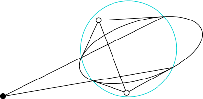
Figure 30: A pair of director points span an axis.

Corollary 5.9.

Through every center of a hyperbolic conic pass two focal lines, two axes, and two directrices.

5.6 Examples

Let us locate foci and directrices for some types of hyperbolic conics. We assume that $\Omega(v,v)=x^{2}+y^{2}-z^{2}$, so that in the Beltrami–Cayley–Klein model in the plane $z=1$ the absolute is the unit circle centered at the origin.

Example 5.10.

By a linear transformation that preserves the absolute, a hyperbolic ellipse can be brought to a canonical form

$$\frac{x^{2}}{a^{2}}+\frac{y^{2}}{b^{2}}=1,\quad 1>a>b$$

The real foci, real focal lines, and real directrices are

$$\left(\pm\sqrt{\frac{a^{2}-b^{2}}{1-b^{2}}},0\right),\quad x=\pm a\sqrt{\frac{1-b^{2}}{a^{2}-b^{2}}},\quad x=\pm a^{2}\sqrt{\frac{1-b^{2}}{a^{2}-b^{2}}}.$$

The directrices are tangent to the absolute if and only if $b=\frac{a}{\sqrt{1+a^{2}}}$. For smaller $b$ the directrices are hyperbolic lines, for larger $b$ they are de Sitter lines, see Figure 31.

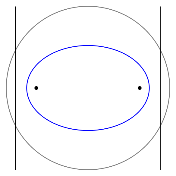
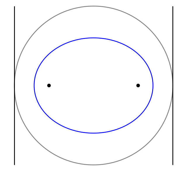
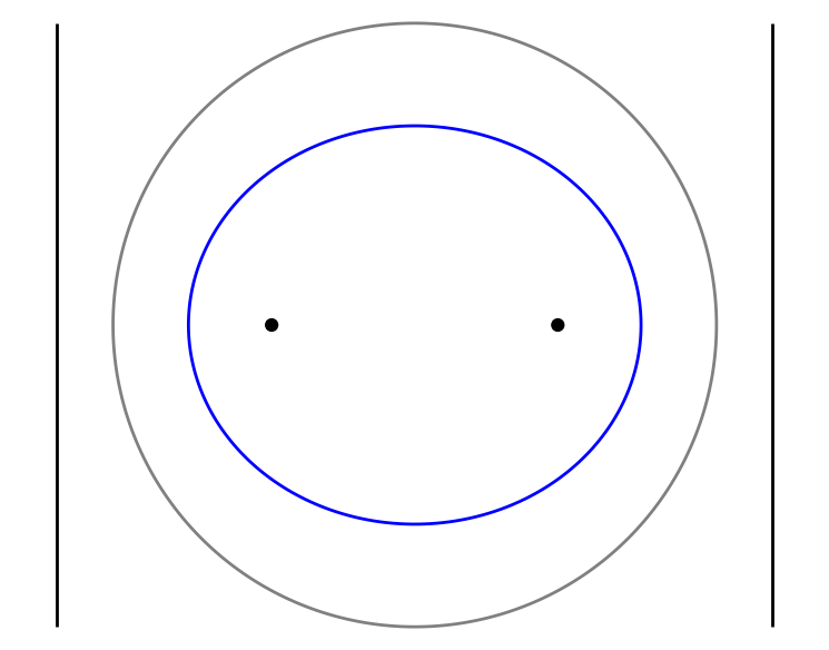
Figure 31: Foci and directrices of hyperbolic ellipses.

Example 5.11.

A semi-hyperbola can be brought to a canonical form

$$ax^{2}-2x+\frac{y^{2}}{b^{2}}=0,\quad|a|<2.$$

The only pair of real foci is

$$F_{1}=\left(\frac{b^{2}}{1-\sqrt{b^{4}-ab^{2}+1}},0\right),\quad F_{2}=\left(\frac{b^{2}}{1+\sqrt{b^{4}-ab^{2}+1}},0\right).$$

The focus $F_{1}$ is a de Sitter point, the focus $F_{2}$ is a hyperbolic point. The corresponding directrices $d_{1}$ and $d_{2}$ are given by equations

$$x=\frac{b^{2}}{ab^{2}-1+\sqrt{b^{4}-ab^{2}+1}},\quad x=\frac{b^{2}}{ab^{2}-1-\sqrt{b^{4}-ab^{2}+1}},$$

respectively. For $a=\frac{1}{b^{2}}$ (that is, when the semi-hyperbola is represented by a circular arc) both directrices are tangent to the absolute, for $a<\frac{1}{b^{2}}$ $d_{1}$ is de Sitter $d_{2}$ is hyperbolic, for $a>b$ $d_{1}$ is hyperbolic and $d_{2}$ is de Sitter, see Figure 32.

If $a=0$ (the semi-hyperbola is represented by a parabola), then $d_{1}=F_{2}^{\circ}$, and $d_{2}=F_{2}^{\circ}$. In this case the semi-hyperbola is the locus of points equidistant from the point $F_{1}$ and the line $d_{1}$, see Example 6.6.

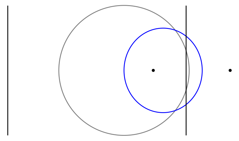
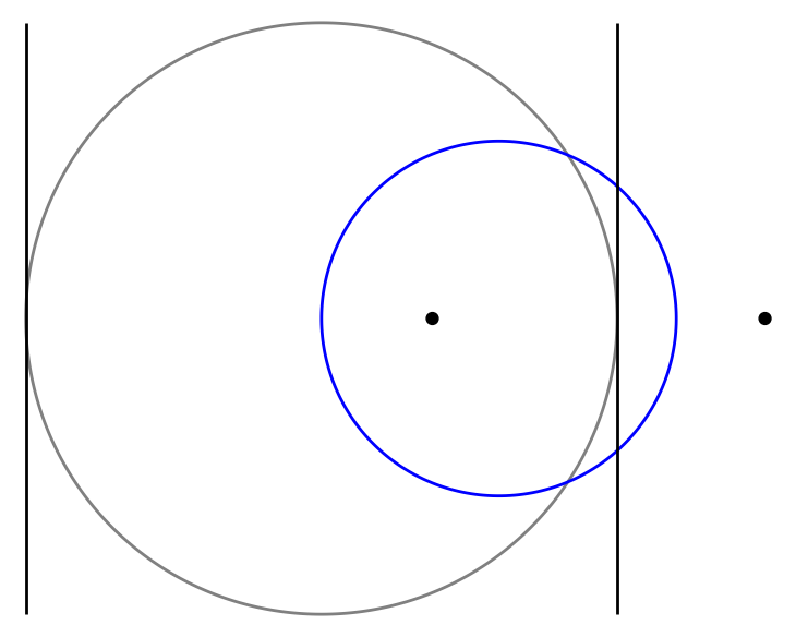
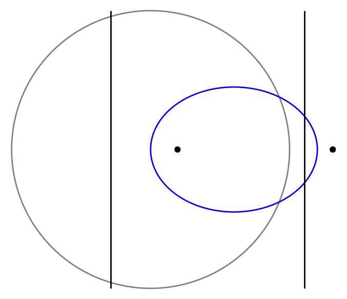
Figure 32: Foci and directrices of semihyperbolas.

Example 5.12.

An elliptic parabola can be brought to a canonical form

$$\frac{(x-(1-a))^{2}}{a^{2}}+\frac{y^{2}}{b^{2}}=1,\quad b^{2}<a<1.$$

(The condition $b^{2}<a$ ensures that the curve stays inside the unit circle.) The only pair of real foci:

$$F_{1}=\left(1-\frac{2(a-b^{2})}{1-b^{2}},0\right),\quad F_{2}=(1,0).$$

The corresponding directrices are given by the equations

$$d_{1}=\left\{x=1+\frac{2a(a-b^{2})}{-a+2b^{2}-ab^{2}}\right\},\quad d_{2}=\{x=1\}.$$

The directrix $d_{1}$ is tangent to the absolute for $a=2b^{2}$, hyperbolic for $a>2b^{2}$, and de Sitter for $a<2b^{2}$.

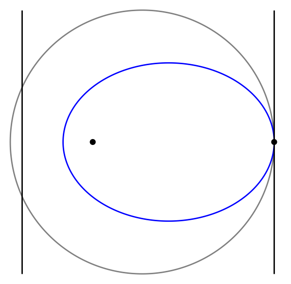
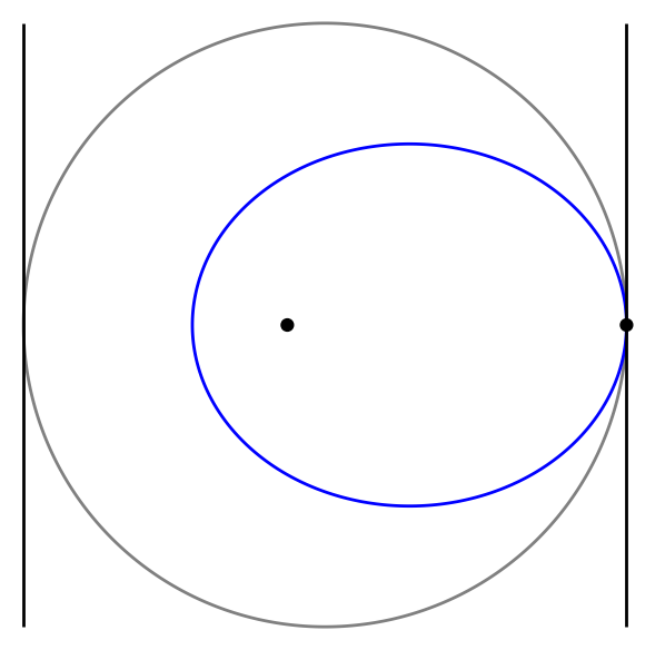
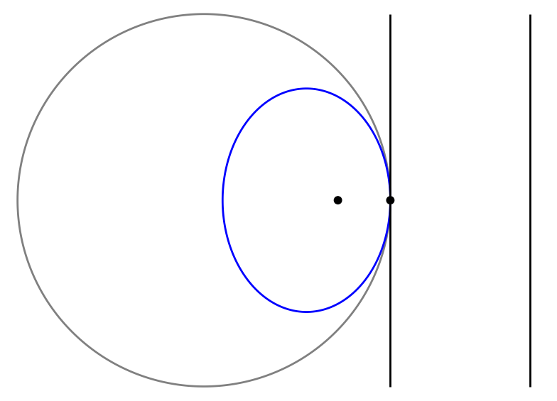
Figure 33: Foci and directrices of elliptic parabolas.

5.7 Families of hyperbolic conics

Since the focal lines of a hyperbolic conic are determined by its intersection points with the absolute, the conics that share the focal lines form a pencil of conics containing the absolute conic. For ellipses and hyperbolas this pencil is determined by four distinct points (some of which can form complex conjugate pairs). For example, if all four points are real, then the pencil is formed by convex and concave hyperbolas and by three pairs of focal lines.

By polarity between foci and focal lines, the confocal conics (those sharing a pair of foci) form a dual pencil. There are several types of confocal nets of hyperbolic conics. The simplest ones are formed by concentric cycles and pencils of lines through their centers.Confocal nets formed by ellipses, hyperbolas, or parabolas are shown on Figures 34 and 35.

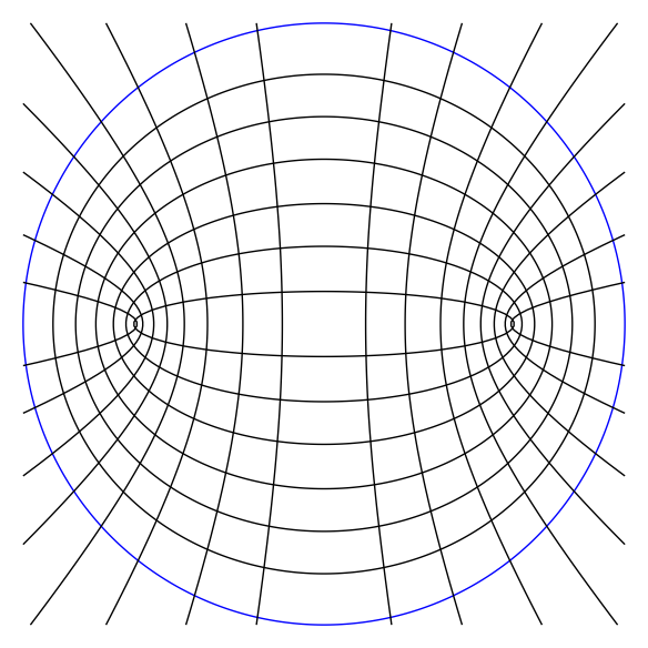
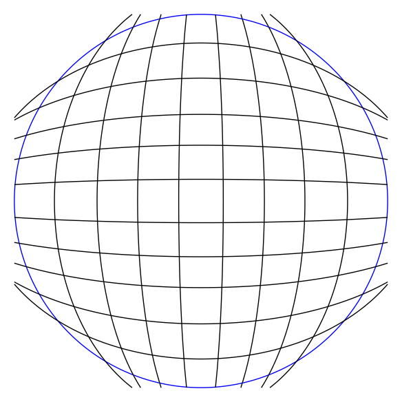
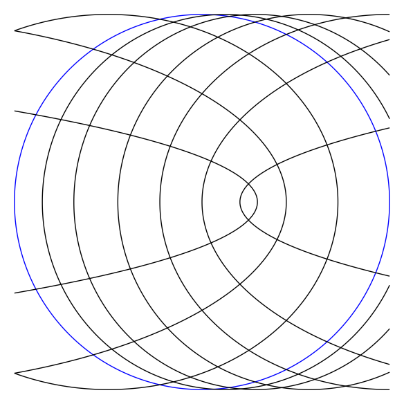
Figure 34: Confocal hyperbolic ellipses and hyperbolas.

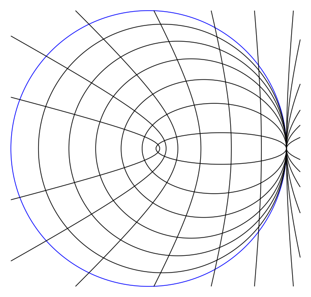
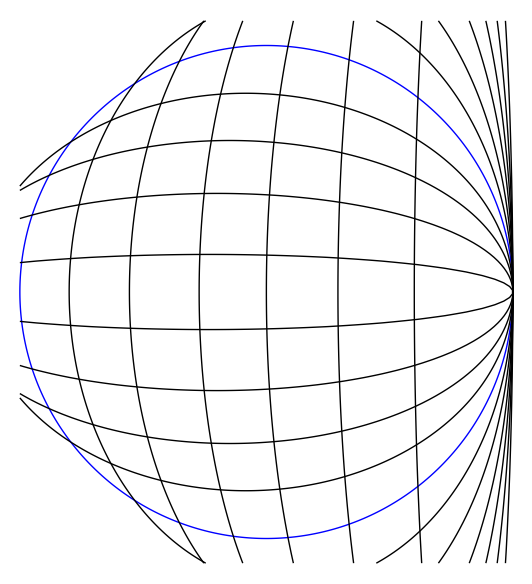
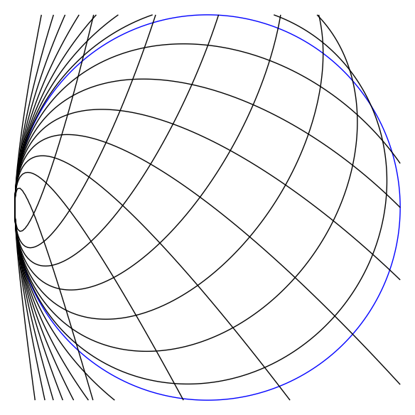
Figure 35: Confocal hyperbolic parabolas.

Conics that share a focus and a corresponding directrix form a double contact pencil, compare Corollary 3.15 in the spherical case.

6 Theorems about hyperbolic conics

6.1 Ivory’s lemma

Similarly to the Euclidean and to the spherical case (see Theorem 4.1), we have the following.

Theorem 6.1 (Ivory’s lemma).

The diagonals in a quadrilateral formed by four confocal hyperbolic conics have equal lengths.

This theorem is proved in [22] by a method similar to that used in the spherical case, see Section 4.1: one finds a homomorphism $F_{\lambda}\colon\mathbb{R}^{3}\to\mathbb{R}^{3}$ that is self-adjoint with respect to $\Omega$ and maps one side of the quadrilateral onto the opposite side.

6.2 Geometric interpretations of the scalar product

This section deals with metric properties of hyperbolic conics. In the proofs it will be more convenient to use the hyperboloid model of the hyperbolic plane. We have

$$\{x\in\mathbb{R}^{3}\mid\Omega(x,x)=-1\}=\mathbb{H}^{2}\cup(-\mathbb{H}^{2}),$$

where $\mathbb{H}^{2}$ and $-\mathbb{H}^{2}$ are two components of the hyperboloid. The distance between two points $x,y\in\mathbb{H}^{2}$ can be computed by the formula

$$\Omega(x,y)=-\cosh\operatorname{dist}(x,y).$$

The hyperboloid of one sheet represents a double cover of the de Sitter plane:

$$\{x\in\mathbb{R}^{3}\mid\Omega(x,x)=1\}=\widetilde{d\mathbb{S}^{2}}.$$

As before, a de Sitter point $x\in\widetilde{d\mathbb{S}^{2}}$ is the pole of a hyperbolic line

$$x^{\circ}=\{y\in\mathbb{H}^{2}\mid\Omega(x,y)=0\}.$$

An advantage of $\widetilde{d\mathbb{S}^{2}}$ over $d\mathbb{S}^{2}$ is that it allows to give a simple description of hyperbolic half-planes:

$$x^{\circ}_{+}=\{y\in\mathbb{H}^{2}\mid\Omega(x,y)\geq 0\},\quad x^{\circ}_{-}=\{y\in\mathbb{H}^{2}\mid\Omega(x,y)\leq 0\}.$$

The scalar product of two de Sitter points computes the angle or the distance between the corresponding hyperbolic lines, and the scalar product of a hyperbolic and a de Sitter point computes the distance between a point and a line. For details, see Lemma 6.2 below.

Finally, there is the isotropic cone, which we divide in two parts

$$\{x\in\mathbb{R}^{3}\mid\Omega(x,x)=0\}=L\cup(-L),$$

where $L$ and $-L$ are one-sided cones asymptotic to $\mathbb{H}^{2}$ and $-\mathbb{H}^{2}$, respectively. For $x\in L$, its polar $x^{\circ}$ is the plane through $x$ tangent to the isotropic cone, which corresponds to a line tangent to the absolute. But there is a more interesting object that one can associate with a point of $L$. Define

$$H_{x}=\{y\in\mathbb{H}^{2}\mid\Omega(x,y)=-1\}.$$

Then $H_{x}$ is a horocycle centered at $x$ (it is not hard to show that the normals to $H_{x}$ pass through $x$). As a curve in $\mathbb{R}^{3}$, $H_{x}$ is a parabola; the central projection makes it an ellipse in the Beltrami–Cayley–Klein model. This ellipse osculates the absolute at the image of the point $x$. The scalar product $\Omega(x,y)$ for $x\in\mathbb{H}^{2}$ and $y\in L$ measures the distance between $x$ and $H_{y}$.

To summarize, every vector in $\mathbb{H}^{2}\cup L\cup\widetilde{d\mathbb{S}^{2}}\subset\mathbb{R}^{3}$ corresponds to a geometric object in the hyperbolic plane: a point, a (co-oriented) line, or a horosphere; the scalar product of two vectors measures the distance between the corresponding objects. An exact formulation is given in the lemma below.

Lemma 6.2.

1. If $x,y\in\mathbb{H}^{2}$, then

   $$\Omega(x,y)=-\cosh\operatorname{dist}(x,y).$$

2. If $x\in\mathbb{H}^{2}$ and $y\in\widetilde{d\mathbb{S}^{2}}$, then

   $$\Omega(x,y)=\sinh\operatorname{dist}(x,y^{\circ}),$$

   where the point-to-line distance $\operatorname{dist}(x,y^{\circ})$ is taken positive if the vectors $x$ and $y$ lie on the same side from the plane $y^{\circ}\subset\mathbb{R}^{3}$, and negative otherwise.

3. If $x\in\mathbb{H}^{2}$ and $y\in L$, then

   $$\Omega(x,y)=-e^{\operatorname{dist}(x,H_{y})},$$

   where the distance to a horosphere is taken to be negative for the points inside the horosphere and positive for the points outside.

4. If $x,y\in\widetilde{d\mathbb{S}^{2}}$, then

   $$\Omega(x,y)=\begin{cases}\cos\angle(x^{\circ},y^{\circ}),&\text{ if }x^{\circ}\cap y^{\circ}\text{ is hyperbolic}\\ \pm 1,&\text{ if }x^{\circ}\cap y^{\circ}\text{ is ideal}\\ \pm\cosh\operatorname{dist}(x^{\circ},y^{\circ}),&\text{ if }x^{\circ}\cap y^{\circ}\text{ is de Sitter}\end{cases}$$

   Here $\angle(x^{\circ},y^{\circ})$ is an angle between the lines $x^{\circ}$ and $y^{\circ}$ occupied by the points $z$ where $\Omega(x,z)$ and $\Omega(y,z)$ have different signs.

5. If $x\in\widetilde{d\mathbb{S}^{2}}$ and $y\in L$, then

   $$\Omega(x,y)=e^{\operatorname{dist}(x^{\circ},H_{y})},$$

   where the distance between a line and a horosphere is the length of the common perpendicular taken with the minus sign if the line intersects the horosphere.

6. If $x,y\in L$, then

   $$\Omega(x,y)=-2e^{\operatorname{dist}(H_{x},H_{y})},$$

   where the distance between two horospheres is the length of the common perpendicular taken with the minus sign if the horospheres intersect.

This is proved via an appropriate parametrization of the line spanned by the points $x$ and $y$, see e. g. [20, 26].

As a simple application of the previous lemma, we can describe the quadratic cones that correspond to hyperbolic cycles.

Lemma 6.3.

For every $c\in\mathbb{R}$ and $p\in\mathbb{R}^{3}$, the quadratic cone

$$\Omega(x,x)+c\cdot\Omega(x,p)^{2}=0$$

corresponds in the hyperbolic-de Sitter plane with the absolute $\Omega$ to a cycle centered at the point $p$. Namely, it describes

$$\begin{cases}\text{a circle with the center }p,&\text{ if }\Omega(p,p)<0,\\ \text{a horocycle with the ideal point }p,&\text{ if }\Omega(p,p)=0,\\ \text{a hypercycle around the line }p^{\circ},&\text{ if }\Omega(p,p)>0.\end{cases}$$

Proof.

The intersection of this quadratic cone with $\mathbb{H}^{2}\subset\mathbb{R}^{3}$ is formed by the points $x$ with $\Omega(x,p)=\mathrm{const}$. Lemma 6.2 implies that these are the points at a constant distance from $p$, if $p\in\mathbb{H}^{3}$, or the points at a constant distance from a horocycle centered at $p$ (hence also a horocycle), if $p\in L$, and the points at a constant distance from the line $p^{\circ}$, if $p\in\widetilde{d\mathbb{S}^{2}}$. ∎

Results of the following sections are essentially due to Story [23]. However, he does not care about the position of foci, focal lines etc., stating the results in terms of $\Omega(x,\cdot)$ only. Therefore we needed to elaborate on the geometric meaning.

6.3 The focus-directrix property

Recall that in the Euclidean case the equation

$$\operatorname{dist}(x,F)=\epsilon\cdot\operatorname{dist}(x,d),$$

where $F$ is a point and $d$ is a line not passing through $F$, determines for $0<\epsilon<1$ an ellipse, for $\epsilon=1$ a parabola, and for $\epsilon>1$ a hyperbola with a focus $F$ and the corresponding directrix $d$. The following theorem gives a similar description of hyperbolic conics.

Theorem 6.4.

Let $S$ be a non-degenerate hyperbolic conic other than a circle, horocycle, and hypercycle. Let $F$ be a non-ideal focus of $S$, and let $d$ be the corresponding directrix. Then the conic consists of all points $x$ that satisfy the equation

$$\delta(F,x)=\epsilon\cdot\delta(d,x)$$ (5)

for some positive constant $\epsilon$, where

$$\delta(F,x)=\begin{cases}\cosh\operatorname{dist}(x,F^{\circ}),&\text{ if }F\text{ is a de Sitter point,}\\ \sinh\operatorname{dist}(x,F),&\text{ if }F\text{ is a hyperbolic point,}\end{cases}$$

$$\delta(d,x)=\begin{cases}\cosh\operatorname{dist}(x,d^{\circ}),&\text{ if }d\text{ is a de Sitter line,}\\ e^{\operatorname{dist}(x,H_{d})},&\text{ if }d\text{ is tangent to the absolute,}\\ |\sinh\operatorname{dist}(x,d)|,&\text{ if }d\text{ is a hyperbolic line.}\end{cases}$$

We need a preparatory lemma.

Lemma 6.5.

Let $p$ be a point not on a conic $Q$. Then we have

$$Q(p,p)Q(x,x)-Q(p,x)^{2}\sim t_{1}(x)\cdot t_{2}(x),$$

where $t_{1}$ and $t_{2}$ are the (possibly imaginary) tangents to $Q$ through $p$.

Proof.

The three conics $Q(x,x)$, $Q(p,x)^{2}$, and $t_{1}(x)\cdot t_{2}(x)$ belong to the same double contact pencil. Thus we have

$$\lambda Q(x,x)+\mu Q(p,x)^{2}+\nu t_{1}(x)t_{2}(x)=0.$$

For $x=p$ the third summand vanishes, which implies $\lambda=-\mu Q(p,p)$, and the lemma is proved. ∎

Proof of Theorem 6.4.

Since the tangents through $F$ to $\Omega$ coincide with the tangents from $F$ to $S$, we have by Lemma 6.5

$$S(F,F)S(x,x)-S(F,x)^{2}\sim\Omega(F,F)\Omega(x,x)-\Omega(F,x)^{2},$$

and hence

$$S(x,x)\sim\Omega(F,F)\Omega(x,x)-\Omega(F,x)^{2}-\lambda S(F,x)^{2}$$

for some $\lambda\in\mathbb{R}$. On the other hand

$$S(F,x)\sim d(x)\sim\Omega(d^{\circ},x),$$

where $d$ is the directrix corresponding to $F$. Hence equation $Q(x,x)=0$ is equivalent to

$$\Omega(F,F)\Omega(x,x)-\Omega(F,x)^{2}=\mu\Omega(d^{\circ},x)^{2},$$

for some $\mu\in\mathbb{R}$, which is in turn equivalent to

$$1-\frac{\Omega(F,x)^{2}}{\Omega(F,F)\Omega(x,x)}=\nu\frac{\Omega(d^{\circ},x)^{2}}{\Omega(x,x)}.$$

Lemma 6.2 provides metric interpretations of the expressions on the left and the right hand side. ∎

It can be shown that the constant in equation 5 is equal to

$$\epsilon=\sqrt{\frac{\Omega(E,E)S(F,d^{\circ})}{S(E,E)\Omega(F,d^{\circ})}},$$

where $E$ is the center of the conic corresponding to the focus $F$, that is the intersection point of the directrix $d$ and the polar $F^{\circ}$ of $F$.

A classification of hyperbolic conics according to the nature of the (focus, directrix) pair and the value of $\epsilon$ seems to be missing in the literature. Below we describe some special cases without going into details.

Let the focus be a hyperbolic point, and the directrix be both hyperbolic. Then the equation

$$\sinh\operatorname{dist}(x,F)=\epsilon\cdot|\sinh\operatorname{dist}(x,d)|$$

describes

$$\begin{cases}\text{for }0<\epsilon<e^{-\operatorname{dist}(d,F)}&\text{an ellipse,}\\ \text{for }\epsilon=e^{-\operatorname{dist}(d,F)}&\text{an elliptic parabola,}\\ \text{for }e^{-\operatorname{dist}(d,F)}<\epsilon<e^{\operatorname{dist}(d,F)}&\text{a semi-hyperbola,}\\ \text{for }\epsilon=e^{\operatorname{dist}(d,F)}&\text{a convex hyperbolic parabola,}\\ \text{for }\epsilon>e^{\operatorname{dist}(d,F)}&\text{a convex hyperbola.}\\ \end{cases}$$

This can be shown by restricting the equation to the line through $F$ perpendicular to $d$.

Example 6.6.

For a point $F$ and a line $d$ not through $F$ the locus of points satisfying

$$\operatorname{dist}(x,F)=\operatorname{dist}(x,d).$$

is a semi-hyperbola whose other focus is the pole of $d$, and the corresponding directrix is the polar of $F$, see Example 5.11. In the Beltrami–Cayley–Klein model in the unit disk, for $F=(c,0)$ and $d=\{x=-c\}$ this semi-hyperbola is described by the equation $x=\frac{1-c^{2}}{4c}y^{2}$.

If the focus $F$ is hyperbolic, and the directrix $d$ is tangent to the absolute or de Sitter, then for small values of $\epsilon$ we get ellipses. As $\epsilon$ increases, the ellipses transition through elliptic parabolas to semihyperbolas, see Examples 5.11 and 5.12.

If for a semihyperbola we take its de Sitter focus, then changing the value of $\epsilon$ will transform the semihyperbola into a concave hyperbola, passing through a (long or wide) concave hyperbolic parabola or, in an exceptional case, through a horocycle.

6.4 Bifocal properties of hyperbolic conics

The following theorem is an analog of Theorem 4.8 about spherical conics.

Theorem 6.7.

1. Let $\ell_{1}$, $\ell_{2}$ be a pair of lines in the hyperbolic-de Sitter plane. For a point $x\in\mathbb{H}^{2}$ let

   $$d_{i}(x)=\begin{cases}\sinh\operatorname{dist}(x,\ell_{i}),&\text{ if }\ell_{i}\text{ is hyperbolic}\\ \cosh\operatorname{dist}(x,\ell_{i}^{\circ}),&\text{ if }\ell_{i}\text{ is de Sitter}\\ e^{\operatorname{dist}(x,H_{i})},&\text{ if }\ell_{i}\text{ is tangent to the absolute.}\end{cases}$$

   Here $H_{i}$ is a horosphere centered at the ideal point $\ell_{i}^{\circ}$, and the distances from a point to a line or to a horosphere are equipped with a sign. Then the locus of points that satisfy an equation of the form

   $$d_{1}(x)\cdot d_{2}(x)=c$$ (6)

   is a hyperbolic conic, and $\ell_{1},\ell_{2}$ is a pair of its focal lines. Conversely, for every pair of focal lines of a hyperbolic conic, the points on the conic satisfy equation (6).

2. Let $p_{1},p_{2}$ be a pair of points in the hyperbolic-de Sitter plane. For a line $\xi$ in the hyperbolic plane let

   $$d_{i}(\xi)=\begin{cases}\sinh\operatorname{dist}(p_{i},\xi),&\text{ if }p_{i}\text{ is hyperbolic}\\ e^{\operatorname{dist}(\xi,H_{i})},&\text{ if }p_{i}\text{ is ideal,}\end{cases}$$

   where $H_{i}$ is a horosphere centered at $p_{i}$. The distances are equipped with a sign. If $p_{i}$ is a de Sitter point, then for all oriented lines $\xi\neq p_{i}^{\circ}$ put

   $$d_{i}(\xi)=\begin{cases}\cos\angle(\xi,p_{i}^{\circ}),&\text{ if }\xi\cap p_{i}^{\circ}\text{ is hyperbolic}\\ \pm 1,&\text{ if }\xi\cap p_{i}^{\circ}\text{ is ideal}\\ \pm\cosh\operatorname{dist}(\xi,p_{i}^{\circ}),&\text{ if }\xi\cap p_{i}^{\circ}\text{ is de Sitter.}\end{cases}$$

   The sign convention must be chosen in such a way that $d_{i}(\xi)$ depends continuously on $\xi$. Then the envelope of the lines that satisfy an equation of the form

   $$d_{1}(\xi)\cdot d_{2}(\xi)=c$$ (7)

   is a hyperbolic conic, and $p_{1},p_{2}$ is a pair of its foci. Conversely, for every pair of foci of a hyperbolic conic, the tangents to the conic satisfy equation (7).

Proof.

Let us prove the first part of the theorem.

Lemma 6.2 implies that

$$d_{1}(x)\cdot d_{2}(x)=\lambda\frac{\Omega(x,\ell_{1}^{\circ})\Omega(x,\ell_{2}^{\circ})}{\Omega(x,x)}$$

for some constant $\lambda$. Therefore equation (6) is equivalent to

$$\Omega(x,x)-\ell_{1}(x)\cdot\ell_{2}(x)=0,$$

where $\ell_{i}$ are certain linear functionals on $\mathbb{R}^{3}$ whose kernels are the lines $\ell_{i}$. Thus the solution set of (6) is the zero set of a quadratic form $Q=\Omega-\ell_{1}\ell_{2}$, that is a hyperbolic conic. If $x$ is a (real or imaginary) intersection point of $Q$ and $\Omega$, then we have $\ell_{1}(x)\cdot\ell_{2}(x)=0$, therefore the lines $\ell_{1}$ and $\ell_{2}$ pass through all four intersection points of $Q$ and $\Omega$. If some of the intersection points coincide (the conic is a parabola or a circle), then either one of the lines is an absolute tangent or both lines pass through the tangency point (this can be shown by passing to the limit). Hence $\ell_{1},\ell_{2}$ is a pair of focal lines of the conic $Q$.

In the opposite direction, let $Q$ be a conic, and let $\ell_{1},\ell_{2}$ be a pair of its focal lines. Then the conics $Q$, $\Omega$, $\ell_{1}\cdot\ell_{2}$ belong to a pencil. Therefore, up to scalar factors we have

$$Q=\Omega-\ell_{1}\cdot\ell_{2}.$$

Thus for all points $x$ on the conic we have $\ell_{1}(x)\cdot\ell_{2}(x)=\Omega(x,x)$, which implies $d_{1}(x)\cdot d_{2}(x)=c$ for some constant $c$.

The proof of the second part is similar. We have

$$d_{1}(\xi)\cdot d_{2}(\xi)=\lambda\frac{\Omega(\xi^{\circ},p_{1})\Omega(\xi^{\circ},p_{2})}{\Omega(\xi^{\circ},\xi^{\circ})}.$$

Therefore equation (7) is equivalent to

$$\Omega(\xi^{\circ},\xi^{\circ})-p_{1}(\xi^{\circ})\cdot p_{2}(\xi^{\circ})=0,$$

where $p_{i}(x)$ is a linear functional proportional to $\Omega(p_{i},x)$. This equation describes a hyperbolic-de Sitter conic; its polar is the envelope of the lines that satisfy equation (7). ∎

Example 6.8.

The locus of points that satisfy

$$\sinh\operatorname{dist}(x,\ell_{1})\cdot\sinh\operatorname{dist}(x,\ell_{2})=c,$$

where $\ell_{1},\ell_{2}$ are two hyperbolic lines, is

• a concave or convex hyperbola or a pair of lines, if the intersection point of $f_{1}$ and $f_{2}$ is non-ideal;

• a concave or convex hyperbolic parabola, if the intersection point of $f_{1}$ and $f_{2}$ is ideal.

Example 6.9.

The locus of points that satisfy $\operatorname{dist}(x,H_{1})+\operatorname{dist}(x,H_{2})=c$, where $H_{1},H_{2}$ are two horocycles, is a hypercycle whose ideal points are the centers of $H_{1}$ and $H_{2}$. The envelope of the lines that satisfy $\operatorname{dist}(\xi,H_{1})+\operatorname{dist}(\xi,H_{2})=c$ is also a hypercycle.

Theorem 6.10.

Let $F_{1},F_{2}$ be a pair of foci of a hyperbolic conic. Then the conic consists of all points $x$ that satisfy an equation of the form

$$|\delta_{1}(x)+\delta_{2}(x)|=\mathrm{const}\quad\text{or}\quad|\delta_{1}(x)-\delta_{2}(x)|=\mathrm{const}.$$

Here the functions $\delta_{i}(x)$ are the distances to the foci or to their polars or to the corresponding horocycles:

$$\delta_{i}(x)=\begin{cases}\operatorname{dist}(x,F_{i}),&\text{ if }F_{i}\text{ is hyperbolic,}\\ \operatorname{dist}(x,F_{i}^{\circ}),&\text{ if }F_{i}\text{ is de Sitter,}\\ \operatorname{dist}(x,H_{i}),&\text{ if }F_{i}\text{ is ideal,}\end{cases}$$

where $H_{i}$ is an arbitrary horocycle centered at $F_{i}$.

Proof.

Let $F$ be a focus of the conic. First assume that $F$ does not belong to the conic (and hence does not belong to the absolute). Denote by $t_{1},t_{2}$ the two absolute tangents through $F$ (which are both real or complex conjugate to each other). By Lemma 6.5 we have

$$Q(F,F)Q(x,x)-Q(F,x)^{2}\sim t_{1}(x)\cdot t_{2}(x)\sim\Omega(F,F)\Omega(x,x)-\Omega(F,x)^{2},$$

which implies

$$Q(x,x)-\frac{Q(F,x)^{2}}{Q(F,F)}=\lambda\left(\Omega(x,x)-\frac{\Omega(F,x)^{2}}{\Omega(F,F)}\right)$$

for some $\lambda\in\mathbb{R}$. To compute $\lambda$, substitute $x=E$, the center conjugate to the axis through $F$. Since the directrix corresponding to $F$ also goes through $E$ (see Lemma 5.8), we have $Q(F,E)=0$, so that $\lambda=\frac{Q(E,E)}{\Omega(E,E)}$.

With the above argument applied to a pair of foci $F_{1}$, $F_{2}$ (of which we assume that both don’t lie on the conic), we obtain

$$Q(x,x)-\lambda\Omega(x,x)=\frac{Q(F_{i},x)^{2}}{Q(F_{i},F_{i})}-\lambda\frac{\Omega(F_{i},x)^{2}}{\Omega(F_{i},F_{i})}\quad\text{ for }i=1,2.$$

Introduce the linear functions $\ell_{1}(x),\ell_{2}(x)$:

$$\ell_{i}(x)=\begin{cases}\frac{\Omega(F_{i},x)}{\sqrt{\Omega(F_{i},F_{i})}},&\text{ if }F_{i}\text{ is de Sitter,}\\ \frac{\Omega(F_{i},x)}{\sqrt{-\Omega(F_{i},F_{i})}},&\text{ if }F_{i}\text{ is hyperbolic.}\end{cases}$$

Since the directrices $Q(F_{i},x)=0$ and the polars $\Omega(F_{i},x)=0$ of the foci meet at the center $E$, each of the linear functions $Q(F_{i},x)$ is a linear combination of $\ell_{1}(x)$ and $\ell_{2}(x)$. Taking into account that $Q(F_{i},F_{i})$ has the same sign as $\Omega(F_{i},F_{i})$, we obtain

$$Q-\lambda\Omega=\begin{cases}(a_{i1}\ell_{1}+a_{i2}\ell_{2})^{2}-\lambda\ell_{1}^{2},&\text{ if }F_{i}\text{ is de Sitter,}\\ -(a_{i1}\ell_{1}+a_{i2}\ell_{2})^{2}+\lambda\ell_{1}^{2},&\text{ if }F_{i}\text{ is hyperbolic.}\end{cases}$$

We now make a case distinction.

1) Both foci are de Sitter. We have

$$(a\ell_{1}+b\ell_{2})^{2}-\lambda\ell_{1}^{2}=Q-\lambda\Omega=(c\ell_{1}+d\ell_{2})^{2}-\lambda\ell_{2}^{2}.$$

Solving this we obtain $\lambda=a^{2}-b^{2}$. Denoting $\mu=\frac{a}{b}$ we see that

$$Q\sim(\mu^{2}-1)\Omega+\ell_{1}^{2}+\ell_{2}^{2}+2\mu\ell_{1}\ell_{2}.$$

Since by Lemma 6.2 $\frac{\ell_{i}(x)}{\sqrt{-\Omega(x,x)}}=\sinh\operatorname{dist}(x,F_{i}^{\circ})=:\sinh\delta_{i}$, equation $Q(x,x)=0$ is equivalent to

$$(1-\mu^{2})+\sinh^{2}\delta_{1}(x)+\sinh^{2}\delta_{2}(x)+2\mu\sinh\delta_{1}(x)\sinh\delta_{2}(x)=0,$$

which factors as

$$(\cosh(\delta_{1}(x)+\delta_{2}(x))-\mu)(\cosh(\delta_{1}(x)-\delta_{2}(x))+\mu)=0.$$

If $\mu>0$, then the conic is described by $|\delta_{1}(x)+\delta_{2}(x)|=c$; if $\mu<0$, then it is described by $|\delta_{1}(x)-\delta_{2}(x)|=c$.

2) Both foci are hyperbolic. In this case we have

$$-(a\ell_{1}+b\ell_{2})^{2}+\lambda\ell_{1}^{2}=Q-\lambda\Omega=-(c\ell_{1}+d\ell_{2})^{2}+\lambda\ell_{2}^{2},$$

which again results in $\lambda=a^{2}-b^{2}$, so that

$$Q\sim(\mu^{2}-1)\Omega-\ell_{1}^{2}-\ell_{2}^{2}-2\mu\ell_{1}\ell_{2}.$$

Now by Lemma 6.2 we have $\frac{\ell_{i}(x)}{\sqrt{-\Omega(x,x)}}=-\cosh\operatorname{dist}(x,F_{i})=:-\cosh\delta_{i}$. Equation $Q(x,x)=0$ is equivalent to

$$\mu^{2}-1+\cosh^{2}\delta_{1}+\cosh^{2}\delta_{2}+2\mu\cosh\delta_{1}\cosh\delta_{2}=0,$$

which factors as

$$(\cosh(\delta_{1}+\delta_{2})+\mu)(\cosh(\delta_{1}-\delta_{2})+\mu)=0.$$

If $\mu>0$, then the conic is empty (in fact, it is the de Sitter ellipse). If $\mu<0$ and $\operatorname{dist}(F_{1},F_{2})<\operatorname{arcosh}(-\mu)$, then the second factor never vanishes, and the conic is described by $\delta_{1}+\delta_{2}=\operatorname{arcosh}(-\mu)$. If $\mu<0$ and $\operatorname{dist}(F_{1},F_{2})>\operatorname{arcosh}(-\mu)$, then the first factor does not vanish, and the conic is described by $|\delta_{1}-\delta_{2}|=\operatorname{arcosh}(-\mu)$.

3) Focus $F_{1}$ is de Sitter, focus $F_{2}$ is hyperbolic. We have

$$(a\ell_{1}+b\ell_{2})^{2}-\lambda\ell_{1}^{2}=Q-\lambda\Omega=-(c\ell_{1}+d\ell_{2})^{2}+\lambda\ell_{2}^{2}.$$

This implies $\lambda=a^{2}+b^{2}$, and we obtain

$$Q\sim(1+\mu^{2})\Omega-\ell_{1}^{2}+\ell_{2}^{2}+2\mu\ell_{1}\ell_{2}.$$

This time we have

$$\frac{\ell_{1}(x)}{\sqrt{-\Omega(x,x)}}=\sinh\operatorname{dist}(x,F_{1}^{\circ}),\quad\frac{\ell_{2}(x)}{\sqrt{-\Omega(x,x)}}=-\cosh\operatorname{dist}(x,F_{2}).$$

Equation $Q(x,x)=0$ is equivalent to

$$1+\mu^{2}+\sinh^{2}\delta_{1}-\cosh^{2}\delta_{2}+2\mu\sinh\delta_{1}\cosh\delta_{2}=0,$$

which factors as

$$(\sinh(\delta_{1}+\delta_{2})+\mu)(\sinh(\delta_{1}-\delta_{2})+\mu)=0.$$

As in the previous case, only one of the factors can vanish (depending on the relation between $\mu$ and $\operatorname{dist}(F_{2},F_{1}^{\circ})$), and the conic is described by one of the equations $\delta_{1}+\delta_{2}=\mathrm{const}$ or $\delta_{1}-\delta_{2}=\mathrm{const}$.

It remains to deal with the case when one or both foci are ideal. If a focus $F$ is ideal, then we claim that

$$Q(x,x)-\lambda\Omega(x,x)=\Omega(F,x)\cdot m(x),$$

where $\lambda=\frac{Q(E,E)}{\Omega(E,E)}$ as before, and $m(x)$ is some linear function. Indeed, the choice of $\lambda$ ensures that the conic $Q-\lambda\Omega$ goes through the point $E$. This point belongs to the line $\Omega(F,x)=0$, which is a common tangent of $Q$ and $\Omega$ at the point $F$, and hence is also a tangent of $Q-\lambda\Omega$ at $F$. It follows that this line is contained in the conic $Q-\lambda\Omega$, and the statement is proved.

Now, assuming that in a pair of foci $(F_{1},F_{2})$ the first one is de Sitter, and the second one is ideal, denote $\ell_{2}(x)=\Omega(F_{2},x)$. We have

$$(a\ell_{1}+b\ell_{2})^{2}-\lambda\ell_{1}^{2}=Q-\lambda\Omega=\ell_{2}\cdot m.$$

It follows that $\lambda=a^{2}$, so that

$$Q\sim\mu^{2}\Omega+2\mu\ell_{1}\ell_{2}+\ell_{2}^{2},$$

where $\mu=\frac{a}{b}$. By Lemma 6.2, we have

$$\frac{\ell_{1}(x)}{\sqrt{-\Omega(x,x)}}=\sinh\delta_{1},\quad\frac{\ell_{2}(x)}{\sqrt{-\Omega(x,x)}}=-e^{\delta_{2}},$$

hence the equation $Q(x,x)=0$ is equivalent to

$$e^{2\delta_{2}}-\mu e^{\delta_{2}+\delta_{1}}+\mu e^{\delta_{2}-\delta_{1}}-\mu^{2}=0,$$

which factors as

$$(e^{\delta_{2}+\delta_{1}}+\mu)(e^{\delta_{2}-\delta_{1}}-\mu)=0.$$

Depending on whether $\mu$ is positive or negative, the conic is described by one of the equations $\delta_{1}+\delta_{2}=\mathrm{const}$ or $\delta_{1}-\delta_{2}=\mathrm{const}$.

The case of an ideal and a hyperbolic focus is similar. If both foci are ideal, then we have

$$Q-\lambda\Omega=a\ell_{1}\cdot\ell_{2},$$

which implies that $Q(x,x)=0$ is equivalent to $\delta_{1}+\delta_{2}=\mathrm{const}$. ∎

Similarly to the spherical case (Theorem 4.6), Theorem 6.10 has a dual that deals with the angles that a tangent to the conic makes with a pair of focal lines (for ultraparallel lines, the angle becomes the length of a common perpendicular). We don’t list all the possibilities here, but here is one interesting particular case. Take two rays in the hyperbolic plane starting at the same point; then the segments with the endpoints on these rays that bound a triangle of constant area envelope a branch of a convex hyperbola, see Figure 36.

Figure 36: A pair of focal lines and a tangent to a convex hyperbola bound a triangle of constant area.

A special case of Theorem 6.10 with $F_{1}$ hyperbolic, $F_{2}$ de Sitter, and zero difference of distances:

$$\operatorname{dist}(x,F_{1})-\operatorname{dist}(x,F_{2}^{\circ})=0$$

is described in Example 6.6.

Theorem 6.10 implies that at every point of the conic the tangent to the conic forms equal angles with the gradients of functions $\delta_{1}$ and $\delta_{2}$. From this we obtain an optical property of the foci, similar to the Euclidean one.

Theorem 6.11.

Let $(F_{1},F_{2})$ be a pair of foci of a hyperbolic conic. Then every light ray originating from $F_{1}$ reflects from the conic in such a way that it either passes through $F_{2}$ or continues a ray originating from $F_{2}$.

The rays originating at an ideal or de Sitter point can be defined in two ways: either as half-lines in a projective model of the hyperbolic-de Sitter plane or as the rays issued by points on a horocycle or on a line in directions orthogonal to that horocycle or a line. Figure 37 shows two examples.

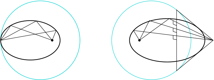
Figure 37: Optical properties of elliptic parabolas and semi-hyperbolas.

A statement dual to Theorem 6.11 says that every segment tangent to the conic and having endpoints on a pair of focal lines is bisected by the point of tangency. Similar to the Euclidean and the spherical case, there is a generalization of Theorem 6.11 and of its dual, see Theorem 4.5. All of these are proved in [23] in a direct way, but the arguments are quite intricate.

Reflective properties of some hyperbolic conics were described in [19] within the Poincare model of the hyperbolic plane.

References

- [1] A. V. Akopyan and A. A. Zaslavsky. Geometry of conics, volume 26 of Mathematical World. American Mathematical Society, Providence, RI, 2007. Translated from the 2007 Russian original by Alex Martsinkovsky.
- [2] M. Berger. Geometry. II. Universitext. Springer-Verlag, Berlin, 1987. Translated from the French by M. Cole and S. Levy.
- [3] W. Blaschke. Eine Verallgemeinerung der Theorie der konfokalen . Math. Z., 27:653–668, 1928.
- [4] M. Chasles. Résumé d’une théorie des coniques sphériques homofocales et des surfaces du second ordre homofocales. Journal de Mathématiques Pures et Appliquées, pages 425–454, 1860.
- [5] M. Chasles and C. Graves. Two geometrical memoirs on the general properties of cones of the second degree, and on the spherical conics. Dublin : For Grant and Bolton, 1841.
- [6] F. Dingeldey. Encyklopädie der mathematischen Wissenschaften mit Einschluss ihrer Anwendungen. Volume 3, T.2, H.1: Kegelschnitte und Kegelschnittsysteme. Leipzig: B. G. Teubner. S. 1–160, 1903.
- [7] F. Dingeldey and E. Fabry. Encyclopédie des sciences mathématiques pures et appliquées. Édition française. Tome III. Vol. 3: Geometrie algébrique plane. Fascicule 1: Les coniques, par F. Dingeldey et E. Fabry. Paris: Gauthier-Villars. S. 1–160, 1911.
- [8] T. E. Faulkner. Projective geometry. Dover Publications, Mineola, NY, reprint of the 2nd edition, 1960 edition, 2006.
- [9] F. Fillastre and A. Seppi. Spherical, hyperbolic and other projective geometries: convexity, duality, transitions. https://arxiv.org/abs/1611.01065. 47 pages.
- [10] K. Fladt. Die allgemeine Kegelschnittsgleichung in der ebenen hyperbolischen Geometrie. J. Reine Angew. Math., 197:121–139, 1957.
- [11] K. Fladt. Die allgemeine Kegelschnittsgleichung in der ebenen hyperbolischen Geometrie. II. J. Reine Angew. Math., 199:203–207, 1958.
- [12] D. Fuchs and S. Tabachnikov. Mathematical omnibus. American Mathematical Society, Providence, RI, 2007. Thirty lectures on classic mathematics.
- [13] G. Glaeser, H. Stachel, and B. Odehnal. The universe of conics. From the ancient Greeks to 21st century developments. Springer Spektrum, Berlin, 2016.
- [14] C. Graves. On certain general properties of cones of the second degree. Proceedings of the Royal Irish Academy (1836-1869), 2:54–57, 1840.
- [15] J. Ivory. On the attraction of homogeneous ellipsoids. Phil. Trans. Royal Soc. London, 99:345–372, 1809.
- [16] I. Izmestiev and S. Tabachnikov. Ivory’s theorem revisited. https://arxiv.org/abs/1610.01384. 51 pages.
- [17] F. Klein. Vorlesungen über nicht-euklidische Geometrie. 3. Aufl. Für den Druck neu bearbeitet von W. Rosemann. Berlin: J. Springer. (Die Grundlehren der mathematischen Wissenschaften in Einzeldarstellung mit besonderer Berücksichtigung der Anwendungsberichte Bd. 26). XII, 326 S. (1928)., 1928.
- [18] L. F. Magnus. Géométrie des surfaces courbes. théorèmes sur l’hyperboloïde à une nappe et sur la surface conique du second ordre. Annales de Gergonne, 16:33–39, 1825.
- [19] R. Perline. Non-Euclidean flashlights. Amer. Math. Monthly, 103(5):377–385, 1996.
- [20] J. G. Ratcliffe. Foundations of hyperbolic manifolds. 2nd ed. New York, NY: Springer, 2nd ed. edition, 2006.
- [21] P. a. Samuel. Projective geometry. Undergraduate Texts in Mathematics. Springer-Verlag, New York, 1988. Translated from the French by Silvio Levy, Readings in Mathematics.
- [22] H. Stachel and J. Wallner. Ivory’s theorem in hyperbolic spaces. Sibirsk. Mat. Zh., 45(4):946–959, 2004.
- [23] W. E. Story. On Non-Euclidian properties of conics. Am. J. Math., 5:358–382, 1883.
- [24] G. S. Sykes and B. Peirce. Spherical conics. Proceedings of the American Academy of Arts and Sciences, 13:375–395, 1877.
- [25] A. Thimm. Integrabilität beim geodätischen Fluß. In Beiträge zur Differentialgeometrie, Heft 2, volume 103 of Bonner Math. Schriften, pages vii+98. Univ. Bonn, Bonn, 1978.
- [26] W. P. Thurston. Three-dimensional geometry and topology. Vol. 1. Ed. by Silvio Levy. Princeton, NJ: Princeton University Press, 1997.
- [27] I. Todhunter. A history of the mathematical theories of attraction and the figure of the earth. From the time of Newton to that of Laplace. In 2 volumes. Reprint of the 1873 original. Cambridge: Cambridge University Press, reprint of the 1873 original edition, 2015.