Non-Markovian dynamics of reaction coordinate in polymer folding

Abstract

We develop a theoretical description of the critical zipping dynamics of a self-folding polymer. We use tension propagation theory and the formalism of the generalized Langevin equation applied to a polymer that contains two complementary parts which can bind to each other. At the critical temperature, the (un)zipping is unbiased and the two strands open and close as a zipper. The number of broken base pairs $n(t)$ displays a subdiffusive motion characterized by a variance growing as $\langle\Delta n^{2}(t)\rangle\sim t^{\alpha}$ with $\alpha<1$ at long times. Our theory provides an estimate of both the asymptotic anomalous exponent $\alpha$ and of the subleading correction term, which are both in excellent agreement with numerical simulations. The results indicate that the tension propagation theory captures the relevant features of the dynamics and shed some new insights on related polymer problems characterized by anomalous dynamical behavior.

I Introduction

Conformational dynamics of biopolymers, such as DNA, RNA and proteins, is a complex process involving a large number of degrees of freedom. Like any other many-body problem, the concept of the reaction coordinate (RC) is often invoked in its coarse grained description. One may be tempted to assume Markovian dynamics for the RC such that the problem is amenable to standard stochastic analysis van Kampen (1995). However, the validity of such a simple approach requires that the RC is the slowest variable and that its characteristic time scale is well separated from all other time scales in the problem. This condition is not easily met in many situations, giving rise to non-Markovian effects and anomalous dynamics.

Anomalous diffusion is an ubiquitous phenomenon observed in a large number of experimental systems or in computer simulations Mandelbrot and Ness (1968); Bouchaud and Georges (1990); Amblard et al. (1996); Krug et al. (1997); Metzler and Klafter (2000); Panja et al. (2009); Amitai et al. (2010); Lizana et al. (2010); Akimoto et al. (2011); Metzler et al. (2014). Characteristic of these systems is a mean squared displacement (MSD) of particle positions (or more generally of some RC) which scales asymptotically in time as $\langle\Delta{\vec{x}}^{2}(t)\rangle\sim t^{\alpha}$ with $\alpha\neq 1$, i.e. deviating from the Brownian motion predictions. The evidence of anomalous dynamics is mostly, both in experiments and simulations, of observational/empirical nature. Due to the complexity of the systems studied it is hard to predict the value of $\alpha$ from theoretical inputs.

In this paper, we investigate the anomalous diffusion of the RC in a simple system with folding dynamics: the (un)zipping in hairpin forming polymers Manghi and Destainville (2016). In this process the polymer contains two complementary parts which can bind to each other and fluctuates between an open (unzipped) and a closed (zipped) conformation. We focus here on the dynamics at the transition temperature where zipped and unzipped state have the same equilibrium free energy. The natural RC for the system is the number of broken base pairs $n(t)$. The time series of $n(t)$ exhibits back and forth fluctuations reminiscent to Brownian motion. Simulations of the mean-square displacement (MSD) reveals the motion is sub-diffusive $\langle\Delta n^{2}(t)\rangle\sim t^{\alpha}$ with $\alpha<1$ Walter et al. (2012).

Here, we clarify the non-Markovian nature of this process using an analysis of the collective dynamics of the polymer, based on the tension propagation along the polymer backbone. A perturbation propagates along the backbone due to the tension transmitted along the chain, generating long range temporal correlations. The theory enables us to provide an analytical estimate of $\alpha$ including the sub-leading term. Our predictions are in very good agreement with the results of computer simulations, which demonstrates the validity of our approach and sheds new insight on related polymer problems characterized by anomalous diffusion.

The theory is based on the Generalized Langevin Equation (GLE) formalism, which is briefly reviewed in Sec. II. The key point is the calculation of the memory kernel entering in the GLE and characterizing the non-Markovian aspects of the dynamics. This calculation is done in Sec. III and allows to estimate both the leading exponent $\alpha$ and the subleading term. In Sec. IV we show that the analytical predictions are in excellent agreement with numerical simulations of the (un)zipping process. Finally, in Sec. V, we present our conclusions and we point out the relation of our results to the problems of tagged monomer motion and polymer translocation.

II Generalized Langevin Equation

Consider a step displacement applied to an appropriate RC ${\vec{z}}(t)$. Let us monitor the subsequent average force ${\vec{f}}(t)$ to keep the given displacement. This protocol can be analyzed by the force balance equation

$$\int_{t_{0}}^{t}d\tau\ \gamma(t-\tau){\vec{v}}(\tau)={\vec{f}}(t)$$ (1)

where ${\vec{v}}(t)=d{\vec{z}}(t)/dt$ and $\gamma(t)$ is the memory kernel (in Markovian systems $\gamma(t)\sim\delta(t)$). In Eq. (1) we may set the lower bound of the time integral as $t_{0}\rightarrow-\infty$ by assuming the system is already in the equilibrium state before the operation is made. In the case of a step displacement ${\vec{u}}$ imposed at $t=0$, i.e., ${\vec{z}}(t+0)={\vec{z}}(t-0)+{\vec{u}}$, we have ${\vec{v}}(t)={\vec{u}}\delta(t)$, the above equation is reduced to

$$u\gamma(t)=f(t)$$ (2)

where we have switched to a scalar notation by noting ${\vec{u}}\parallel{\vec{f}}$ in isotropic system.

To connect the average stress relaxation with the anomalous fluctuating dynamics, we need to look at each realization of the stochastic processes by adding the thermal noise term ${\vec{\xi}}(t)$ to the right-hand side of Eq. (1). The noise has zero mean $\langle\xi_{\text{i}}(t)\rangle=0$, and it is related to the memory kernel via the fluctuation-dissipation theorem (FDT) $\langle\xi_{\text{i}}(t)\xi_{\text{i}}(\tau)\rangle=k_{B}T\gamma(|t-\tau|)\delta_{\text{i}j}$. The equivalent expression of the Generalized Langevin Equation (GLE) is

$${\vec{v}}(t)=\int_{t_{0}}^{t}d\tau\ \mu(t-\tau){\vec{f}}(\tau)+{\vec{\eta}}(t)$$ (3)

where $\mu(t)$ is the mobility kernel with the FDT $\langle\eta_{\text{i}}(t)\eta_{\text{j}}(\tau)\rangle=k_{B}T\mu(|t-\tau|)\delta_{\text{i}j}$ Saito and Sakaue (2015); Panja (2010); Vandebroek and Vanderzande (2017); Sakaue (2016). In the next section a power-law decaying memory function $\gamma(t)\sim t^{-\alpha}$ in the case of polymer pulling is derived from polymer tension propagation arguments. From this one derives $\mu(t)\sim-t^{\alpha-2}$ (for details see Appendix A). In the unbiased case ${\vec{f}}(t)=0$, the MSD can be derived after integration of the velocity correlation function $\langle{\vec{v}}(t)\cdot{\vec{v}}(s)\rangle=\langle{\vec{\eta}}(t)\cdot{\vec{\eta}}(s)\rangle$ twice with respect to time, yielding $\langle\Delta{\vec{z}}(t)^{2}\rangle\sim t^{\alpha}$, i.e., the stress relaxation exponent characterizing the decay of the memory kernel $\gamma(t)$ is equal to the MSD exponent.

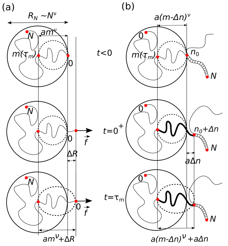
Figure 1: Illustration of the differences in tension propagation between a polymer pulled by one end (a) and a zipping polymer (b). In both cases to calculate the memory kernel one starts from an equilibrated conformation and introduces a perturbation. (a) Pulling occurs at time $t=0$. At time $t=\tau_{m}$ the tension front has reached the monomer $m$. Here the deformation $\Delta R$ is fixed by the initial pulling. (b) In zipping peeling of $\Delta n$ monomers occurs at a time $t=0$. At a time $t=\tau_{m}$ the perturbed part of the chain involves $m(t)$ monomers counting from the new fork point (thick line in the figure). The deformation $\Delta R_{m}$ of the polymer is equal to the difference between the actual size of this perturbed part and its equilibrium size (Eq. 7).

III Memory kernel for zipping dynamics

Before dealing with the more complex case of zipping polymers, it is useful to recall some known results Sakaue et al. (2012); Saito and Sakaue (2015) for a simpler case of polymer pulling (see Fig. 1(a)). Let us suppose that one end of an equilibrated polymer is displaced by $\Delta x$ at $t=0$ and that the position of that monomer is kept fixed. This operation produces a stretching of the end part of the chain. Through tension propagation the polymer relaxes to a new equilibrium state shifted with respect to the original position. The longest relaxation time is $\tau_{N}\simeq\tau_{0}N^{z\nu}$, where $\tau_{0}$ is a monomer time scale, $\nu\simeq 0.588$ is the Flory exponent and the $z=2+1/\nu$ is the dynamical exponent (we consider here the free draining case, if hydrodynamic interactions are taken into account $z=3$). At a time $t<\tau_{N}$ only $m(t)$ monomer close to the displaced end are stretched, while the remaining $N-m(t)$ at the opposite end do not yet feel the displacement operation. The longest relaxation time for a fragment containing $m$ monomers is $\tau_{m}\simeq\tau_{0}m^{\nu z}$, from which one finds

$$m(t) \simeq \left(\frac{t}{\tau_{0}}\right)^{\frac{1}{\nu z}}$$ (4)

which gives how $m$ grows in time. To keep the end monomer at a fixed position one needs to apply a force $f(t)$ which can be estimated using polymer entropic elasticity. An equilibrated polymer stretched by $\Delta x$ exerts a force at its two ends which is equal to:

$$f \simeq \frac{k_{B}T}{\langle R^{2}\rangle}\Delta x$$ (5)

where $\langle R^{2}\rangle$ indicates the average of the squared end-to-end distance. Applying the previous relation to the stretched $m(t)$ monomers, for which $\langle R^{2}\rangle\simeq a^{2}m^{2\nu}$ and using Eq. (4) we obtain

$$\gamma(t)=\frac{f(t)}{\Delta x} \simeq \frac{k_{B}T}{a^{2}}\left(\frac{t}{\tau_{0}}\right)^{-2/z}$$ (6)

where we used Eq. (2) for a step displacement equal to $\Delta x$. Equation (6) gives the memory kernel associated to the step displacement of a polymer end. According to the discussion of the previous section the decay exponent of $\gamma(t)$ is equal to the MSD exponent. Hence we obtain $\alpha=2/z$. For an ideal Rouse chain for which $z=4$ ($\nu=1/2$), one obtains a tagged monomer diffusion with MSD scaling as $\Delta\vec{x}^{\,2}(t)\sim t^{1/2}$, which is in agreement with the exact solution from Rouse dynamics Doi and Edwards (1988). More generally the tension propagation dynamics leads to a subdiffusive behavior with $\alpha=2\nu/(1+2\nu)<1$, which turns into ordinary diffusion at times $t>\tau_{R}$.

We turn now to the case of zipping dynamics. Let us assume that the polymer is in equilibrium with $n_{0}$ bonds from the tail being in unzipped state, while the remaining $N-n_{0}$ bonds are zipped, i.e., the monomer’s label at the fork point is $n(t)=n_{0}$ ($t<0$). Consider now an instantaneous break of $\Delta n(={\mathcal{O}}(1))$ zipped pairs at the fork point creating $\Delta n$ additional unzipped monomer pairs. This operation produces (i) the change of the reaction coordinate $n(t)=n_{0}\rightarrow n_{0}+\Delta n$ and (ii) the displacement of the position of the fork in real space ${\vec{r}}(n_{0},0)\rightarrow{\vec{r}}(n_{0}+\Delta n,0)$, where ${\vec{r}}(n,t)$ is the position of the monomer $n$ at time $t$ (Fig. 1(b)). As in the pulling problem the entire chain cannot respond to the break of $\Delta n$ bonds all at once. At time $t$ smaller than the longest relaxation time of the polymer only a finite section, i.e., $m(t)$ bonds given close to the fork point respond to the perturbation.

The deformation of such a responding part of the chain can be evaluated as (Fig. 1(b))

$$\Delta R_{m}(t) \simeq a\Delta n+a\{m(t)-\Delta n\}^{\nu}-am(t)^{\nu}$$ (7)

$$\simeq a[\Delta n-\nu\Delta nm(t)^{\nu-1}]$$

where we have taken $m(t)\gg\Delta n$ and expanded to lowest order in $\Delta n$. The previous equation can be understood as follows. There are $m(t)$ monomers in the part of the unzipped arm which is under tension (thick line in Fig. 1(b)). The equilibrium radius of this part would be $am(t)^{\nu}$. However at time $t$ the actual size is $a\Delta n+a\{m(t)-\Delta n\}^{\nu}$ because the average position of the monomer at the tension front is not yet affected by the peeling at this time scale. The total size is the sum of the unperturbed size of $m(t)-\Delta n$ monomers and of the peeled part which is $a\Delta n$. The deformation $\Delta R_{m}(t)$ is then obtained by subtracting the actual radius of the $m(t)$ monomers and the equilibrium value, which leads to Eq. (7).

The growth of $m(t)$ in time is governed by the tension propagation dynamics of Eq. (4). The force necessary to hold the fork point to the new position $n_{0}+\Delta n$ can be estimated again from entropic elasticity (Eq. (5)) as

$$f(t) \simeq \frac{k_{B}T}{\langle R^{2}(t)\rangle}\Delta R_{m}(t)$$ (8)

$$\simeq \frac{k_{B}T}{a}\Delta n\left[\left(\frac{t}{\tau_{0}}\right)^{-2/z}-\nu\left(\frac{t}{\tau_{0}}\right)^{-\frac{1+\nu}{\nu z}}\right]$$

Dividing by $a\Delta n$ we obtain the memory kernel with a leading $t$ behavior as in Eq. (6), but now the analysis unveils the presence of a sub-leading term. The calculation of the MSD which follows from Eq. (8) is given in the Appendix A, where the full calculation of $\gamma(t)$ is presented including the subleading term. The final result for the RC dynamics is

$$\langle\Delta n^{2}(t)\rangle\sim t^{2/(\nu z)}\left(1+Ct^{-(1-\nu)/(\nu z)}\right)$$ (9)

with $C$ a positive constant.

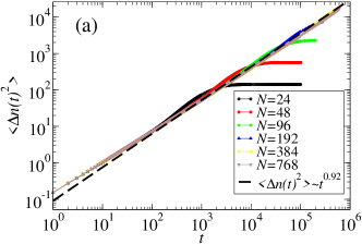
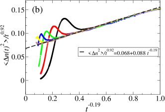
Figure 2: (a) The mean-square displacement $<\Delta n(t)^{2}>$ of the reaction coordinate (fork location along the chain) is plotted versus time for different sizes. The symbols are obtained for simulations with different sizes (from Walter et al. (2012)). The dashed line is the theoretical prediction with an exponent 0.92. The deviation of the MSD from the leading term at short time is explained by the subleading term in Eq.(9). (b) Correction to scaling $\Delta n(t)^{2}/t^{0.92}$ plotted versus $t^{-0.19}$. According to Eq.(9), the resulting curve should fit linearly. Remarkably, even the numerical value of the slope of the corrections are in good agreement with theory. For both the leading and first order correction to scaling, the numerics are in very good agreement with theoretical predictions.

IV Numerical Results

The model used in the simulations is discussed in details in Ref. Walter et al. (2012) and was also employed in previous studies of renaturation dynamics Ferrantini et al. (2010). We consider two strands with $N$ monomers which are joined to a common monomer, labeled with $i=N$, while we use an index $i=1\ldots N$ to label the monomers on the two strands. Only monomers with the same index $i$ on the two strands can bind with binding energy $\varepsilon$. The dynamics consists of lattice corner-flips or end-flips local moves which are randomly generated by a Monte Carlo algorithm. This algorithm was shown to reproduce the Rouse model dynamics in previous studies Ferrantini and Carlon (2011) and represents an interesting and efficient alternative to the more commonly used Langevin dynamics for polymers in the continuum.

A Monte Carlo move not respecting mutual or self-avoidance between the two strands is rejected. A move binding two monomers on the opposite strands is always accepted, while the opposite move of unbinding is accepted with a probability $\exp(-\beta\varepsilon)<1$, where $\beta=1/k_{B}T$ is the inverse temperature. The algorithm hence satisfies detailed balance. The temperature is tuned to the critical value $\beta=\beta_{c}$, which is very accurately known as it relies on previous high precision data about polymers on an fcc lattices Ishinabe (1989). In addition in the model bubbles are not allowed to form so the dynamics is strictly sequential as in a zipper.

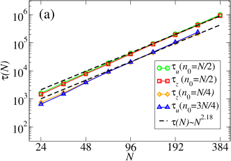
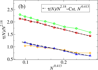
Figure 3: (a) The zipping and unzipping time $\tau_{z}$ and $\tau_{u}$, respectively, are plotted versus the polymer length for different initial conditions ($n_{0}=N/4,$ $N/2$ and $3N/4$). Symbols are results from simulations, and Eq.(10). The analytical estimate of the exponent $2.18$ is in good agreement with the numerics for large sizes. (b) $\tau/N^{2.18}$ is plotted versus the first order correction to scaling $t^{-0.413}$. The resulting curve is expected to be a straight line with a negative slope. Both leading term and first order correction are in good agreement with the numerics, independent from the initial value of $n_{0}$.

A simulation run is initialized by setting the fork point to $n(t=0)=N/2$, so that monomers $0\leq i\leq N/2$ are unbound and $i>N/2$ are bound. The initial configuration is equilibrated by sufficiently long Monte Carlo runs while keeping the fork point fixed (see Appendix B). After equilibration, the constraint is released and the actual simulation is started. The fork point performs a stochastic back and forth motion along the polymer backbone until one of the two ends is reached and the simulation is stopped. We monitor in particular the MSD $\langle\Delta n^{2}(t)\rangle$ and the average duration time of the process $\tau$.

The analysis of Ref. Walter et al. (2012) showed that the dynamics is well-described by a fractional brownian motion (fBm) characterized by a Hurst exponent $H=0.44(1)$ (recall that in fBM the Hurst exponent is linked to the MSD exponent by the relation $\alpha=2H=0.88(2)$ and that the fBm is described by a GLE). The analytical prediction of Eq. (9) is $\alpha=2/(\nu z)=0.92$, which is somewhat higher that the numerical value of Ref. Walter et al. (2012). Figure 2(a) shows a plot of the MSD for lattice polymers of lengths up to $N=768$ and averaged over $\sim 5\cdot 10^{5}$ realizations. The dashed line in Fig. 2(a) is the analytical prediction. The data converge to this prediction for sufficiently long times, with some deviations close to the saturation level (obviously the MSD cannot grow beyond the squared half total length of the strands). At short times there is a visible deviation from the analytical prediction.

In order to test the validity of Eq. (9) we plot in Fig. 2(b) the quantity $\langle\Delta n^{2}(t)\rangle t^{-0.92}$ vs. $t^{-(1-\nu)/(\nu z)}=t^{-0.19}$. The MSD plotted in these rescaled unit is expected to show a linear behavior, which is indeed observed in Fig. 2(b). Also it is important to note that the theory predicts a positive coefficient $C>0$ in Eq. (9), as discussed in Appendix A, and this is indeed consistent with the numerics. Moreover, a fit of the correction gives $\langle n(t)^{2}\rangle/t^{0.92}=0.068(1+C\,t^{-0.19})$ where the prefactor $C=1.294$ is in good agreement with the theoretical prediction $1.726$ given by Eq.(29). Hence we can conclude that the numerical data are in excellent agreement with the tension propagation theory predictions.

Additional support to the theory is obtained from the analysis of the average time $\tau$ to fully zip or unzip as a function of the polymer length $N$, see Fig.3. The system is prepared in different initial conditions. For $n_{0}=N/2$, we sample both the unzipping time $\tau_{u}$ and the zipping time $\tau_{z}$ depending which end $N$ or 0 is reached first, respectively. We also sample the zipping time for $n_{0}=N/4$, and the unzipping time for $n_{0}=3N/4$. This time is expected to be an increasing function of the strands length $N$. From Eq.(9) one obtains the asymptotic scaling $\tau\sim N^{\nu z}$. This result can be extended to the next order correction from the analysis of Eq. (9)

$$\tau\sim N^{\nu z}\left(1-DN^{-(1-\nu)}+\ldots\right)$$ (10)

with $D>0$. To confirm it, we first present a log-log plot of $\tau$ vs. $N$ in Fig. 3(a), which shows some deviations from the asymptotic behavior $\tau\sim N^{\nu z}$. We then show a plot of $\tau N^{-\nu z}$ vs. $N^{-(1-\nu)}$ in Fig. 3(b). The rescaled data follow a straight line with a negative slope in very good agreement with the prediction of Eq. (10). We do not observe any change in the dynamical scaling for different initial conditions as it has been observed in the related system of protein search on DNA Lange et al. (2015).

V Conclusion

The anomalous dynamics in polymers originates from growth of the cooperatively moving domain, i.e., tension propagation along the chain: a perturbation on a given position propagates along the polymer backbone creating a viscoelastic memory effect for the motion of individual monomers. A theoretical framework of tension propagation has been mostly developed in the past years for the nonequilibrium dynamics of polymers ,i.e. the analysis of driven polymer translocation Sakaue (2007, 2010); Ikonen et al. (2012) and the polymer stretching process Sakaue et al. (2012); Saito and Sakaue (2015); Rowghanian and Grosberg (2012); Vandebroek and Vanderzande (2014, 2017). In near-equilibrium (or unbiased) situations, the essential physics is also given by the growing length scale of the cooperative motion as the source of anomalous dynamics, for which the scaling form of the tension propagation is determined by an equilibrium argument, see Eq.4. In the unbiased translocation dynamics it is a monomer exchange across the pore that generates a long range decay of the memory kernel Panja et al. (2007); Panja (2010); Sakaue (2016), while in the tagged monomer motion the same effect is due to the spatial displacement by pulling Saito and Sakaue (2015); Panja (2010); Sakaue (2013).

The (un)zipping dynamics analyzed in this paper can be understood as a hybrid of the above two processes. It is the monomer exchange $\Delta n$ (cf. Fig. 1) between zipped and unzipped sections which creates a long range temporal memory leading to a power-law decaying memory kernel as in Eq. (8). Inspecting the elementary process, we see that the first term in the RHS of Eq. (7) reflects the process entailing the spatial displacement ${\vec{r}}(n_{0},0)\rightarrow{\vec{r}}(n_{0}+\Delta n,0)$, while the second term concerns the change in $\Delta n$ without spatial displacement. The latter is reminiscent to the translocation process entailing the monomer exchange across the pore, while the spatial position of the RC is fixed at the pore site.

The present formalism enabled us to extract the anomalous diffusion characteristics of the RC including the subleading behavior

$$\langle\Delta n^{2}(t)\rangle\sim t^{\alpha}\left(1+Ct^{-\alpha_{1}}+\ldots\right)$$ (11)

with analytical expressions for $\alpha$ and $\alpha_{1}$ which are found to match very well the numerical simulation data. Since the dominant source of the tension generation comes from the spatial displacement of the RC, a process equivalent to pulling operation (the first term in the RHS of Eq. (7)), the asymptotic anomalous diffusion exponent $\alpha=2/(\nu z)$ is controlled by that of the tagged monomer diffusion, see Eq. (8), while the subleading exponent $\alpha-\alpha_{1}=(1+\nu)/(\nu z)$ coincides with that expected for the unbiased polymer translocation (see Eq. (9) in Ref. Sakaue (2016)). Note, however, that the translocation problem is complex because of a series of factors (post-propagation behavior, interaction with the pore), and simulations, at least in the unbiased case, are still controversial Chuang et al. (2001); de Haan and Slater (2012); Palyulin et al. (2014); Sakaue (2016).

From a broader perspective, we repeat once more the caution on the RC based coarse grained description. The validity of the assumption leading to the Markovian dynamics is generally dependent on the time scale at hand (say, observation), but as we have shown here, there would exist for the dynamics of long polymers a broad time window, in which collective dynamics among degrees of freedom with varying time scale manifests. Indeed, the Markovian description is valid only on the time scale coarser than the longest relaxation time $\tau_{N}\simeq\tau_{0}N^{\nu z}$ of the molecule. Therefore, the slow dynamics is a generic feature in high molecular weight macromolecules, and this implies that on the time scale $(t<\tau_{N})$ relevant to the conformational dynamics, only the partial section of a chain can be equilibirated. Our present theory utilizes equilibrium properties of such an equilibriated section, whose size evolves in time along with the tension propagation. This allows us to clarify the stress relaxation and the anomalous dynamics of RC due to the viscoelastic response. The resulting non-Markovian dynamics should be of pronounced importance in the context of biopolymer functions. Although more work is necessary to fully unveil the consequences, our analytical argument for the MSD is regarded a first step toward such an ambitious goal.

Away from the critical point, at low temperatures, the hairpin folding process exhibits out-of-equilibrium characteristics Frederickx et al. (2014) which resembles scaling behavior observed in DNA hairpin experiments Neupane et al. (2012). That case is reminiscent of polymer translocation driven by external bias  Sakaue (2007, 2010); Lehtola et al. (2009); Bhattacharya and Binder (2010); Ikonen et al. (2012); Sakaue (2016). Here again, a key physics lies in the tension propagation, the dynamics of which bears distinctive features not seen in the unbiased regime discussed in this work.

*

Appendix A The correction to scaling behavior

We give here the full derivation of the calculation of the MSD including the subleading corrections. The calculation consists of two steps. Firstly we determine the mobility kernel $\mu(t)$ and from it, using the FDT, we obtain the MSD.

A.1 Mobility Kernel

Taking the Laplace transforms of Eqs. (1) and (3) one obtains the following relation:

$$\hat{\mu}(s)=\frac{1}{\hat{\gamma}(s)}$$ (12)

(generalizing the relation between mobility and friction). In the previous equation $\hat{\gamma}(s)$ and $\hat{\mu}(s)$ are the Laplace transforms of $\gamma(t)$ and $\mu(t)$, respectively. In what follows we calculate the Laplace transform of the memory kernel $\hat{\gamma}(s)$ and then obtain $\hat{\mu}(s)$ from Eq. (12). Finally we use the inverse Laplace transform to obtain $\mu(t)$. This can be readily done for a pure power law function $\gamma(t)=t^{-\alpha}$: its Laplace transform is $\hat{\gamma}(s)=\Gamma(1-\alpha)s^{\alpha-1}$, where $\Gamma(z)$ is the Euler gamma function. Therefore, neglecting the prefactor, $\hat{\mu}(s)\sim s^{1-\alpha}$ which leads to $\mu(t)\sim t^{\alpha-2}$. This is the result mentioned at the end of Section II.

Let us start now from the memory kernel which includes a subleading correction at long times:

$$\gamma(t)\simeq\frac{k_{B}T}{a^{2}}t^{-2/z}\left[1-\nu t^{-\frac{\nu+1}{\nu z}+\frac{2}{z}}\right]$$ (13)

where the time is made dimensionless with the unit $\tau_{0}$. Its Laplace transform is:

$$\hat{\gamma}(s)=\frac{k_{B}T}{a^{2}}\left[\Gamma\left(1-\frac{2}{z}\right)s^{2/z-1}-\nu\Gamma\left(1-\frac{\nu+1}{\nu z}\right)s^{\frac{\nu+1}{\nu z}-1}\right]=\frac{k_{B}T}{Aa^{2}}s^{2/z-1}\left[1-Bs^{\frac{\nu+1}{\nu z}-2/z}\right]$$ (14)

where we have introduced

$$B\equiv\nu\frac{\Gamma(1-\frac{\nu+1}{\nu z})}{\Gamma(1-2/z)}>0$$ (15)

and

$$A^{-1}\equiv\Gamma(1-2/z)>0$$ (16)

From (12) and (14) we get

$$\hat{\mu}(s)=\frac{a^{2}}{k_{B}T}As^{1-2/z}\left[1-Bs^{\frac{\nu+1}{\nu z}-2/z}\right]^{-1}$$ (17)

The inverse Laplace transform can be calculated using the Mittag-Leffler function Haubold et al. (2011). However, in order to avoid possible convergence issues we will only calculate $\mu(t)$ in the long time limit, which corresponds to the small $s$ approximation of (17). In that limit we get

$$\hat{\mu}(s)=\frac{a^{2}}{k_{B}T}A\left[s^{-\kappa}+Bs^{-\epsilon-\kappa}+\ldots\right]$$ (18)

where $\epsilon=2/z-(\nu+1)/(\nu z)<0$ and $\kappa=2/z-1<0$. The inverse Laplace transform of (18) is given by

$$\mu(t)=\frac{a^{2}}{k_{B}T}A\left[\frac{t^{\kappa-1}}{\Gamma(\kappa)}+B\frac{t^{\epsilon+\kappa-1}}{\Gamma(\epsilon+\kappa)}\right]$$ (19)

A.2 Mean squared displacement of the reaction coordinate

In absence of forces Eq. (3) becomes

$$\vec{v}(t)=\vec{\eta}(t)$$ (20)

where

$$\langle\eta_{\text{i}}(t)\eta_{\text{j}}(s)\rangle=k_{B}T\mu(|t-s|)\delta_{\text{ij}}$$ (21)

From (20) we get for the mean squared displacement (MSD) $\Delta\vec{x}^{\,2}(t)=\langle(\vec{x}(t)-\vec{x}(0))^{2}\rangle$

$$\Delta\vec{x}^{\,2}(t)=3\int_{0}^{t}\int_{0}^{t}\langle\eta(t_{1})\eta(t_{2})\rangle dt_{1}dt_{2}$$ (22)

Therefore using (21) and (19) we get

$$\Delta\vec{x}^{\,2}(t)=3a^{2}A\int_{0}^{t}\int_{0}^{t}\left[\frac{|t_{1}-t_{2}|^{\kappa-1}}{\Gamma(\kappa)}+B\frac{|t_{1}-t_{2}|^{\epsilon+\kappa-1}}{\Gamma(\epsilon+\kappa)}\right]dt_{1}dt_{2}$$ (23)

Integrals of the type

$$I=\int_{0}^{t}\int_{0}^{t}|t_{1}-t_{2}|^{\sigma}dt_{1}dt_{2}$$ (24)

are easily performed. First, from the symmetry between $t_{1}$ and $t_{2}$ we get

$$I=2\int_{0}^{t}(\int_{0}^{t_{1}}(t_{1}-t_{2})^{\sigma}dt_{2})dt_{1}$$ (25)

and then switching to $y=t_{2}/t_{1}$

$$I=2\int_{0}^{t}t_{1}^{\sigma+1}dt_{1}\int_{0}^{1}(1-y)^{\sigma}dy=\frac{2t^{2+\sigma}}{(2+\sigma)(1+\sigma)}$$ (26)

provided $\sigma>-1$. Otherwise we get a divergence at the origin. However, physically we can always introduce a small cutoff and take the initial time to be some small time $t_{\epsilon}$. This will add a constant to the result (26).

Inserting (26) into (23) we get

$$\Delta\vec{x}^{\,2}(t)=6a^{2}A\left[\frac{t^{\kappa+1}}{\kappa(\kappa+1)\Gamma(\kappa)}+B\frac{t^{1+\kappa+\epsilon}}{\Gamma(\epsilon+\kappa)(\kappa+1+\epsilon)(\kappa+\epsilon)}+\ldots\right]$$

Using the relation $z\Gamma(z)=\Gamma(z+1)$,

$$\Delta\vec{x}^{\,2}(t)=6a^{2}A\left[\frac{t^{1+\kappa}}{\Gamma(\kappa+2)}+B\frac{t^{\epsilon+\kappa+1}}{\Gamma(\kappa+\epsilon+2)}+\ldots\right]$$ (27)

We next go from motion in physical space to motion in monomer space throught the relation $\Delta\vec{x}^{\,2}(t)\sim[\Delta n^{2}(t)]^{\nu}$. Inserting in (27) gives our final result from which one can read off the leading correction to the asymptotic scaling

$$\Delta n^{2}(t)\sim t^{(1+\kappa)/\nu}\left[1+\frac{B\Gamma(\kappa+2)}{\nu\Gamma(\kappa+\epsilon+2)}t^{\epsilon}+\ldots\right]$$ (28)

Inserting $\nu=.588$ then gives

$$\langle\Delta n^{2}(t)\rangle\sim t^{.92}\left[1+C\,t^{-0.19}+\ldots\right]$$ (29)

where the prefactor $C$ in front of the correction is positive, whose value is calculated as $C\approx 1.695B\approx 1.726$ for the present case ($z=1+2\nu$ with $\nu=0.588$).

Appendix B Numerical simulations

The numerical model used in this article was also used in studies of renaturation dynamics Ferrantini et al. (2010) and zipping dynamics Ferrantini and Carlon (2011); Walter et al. (2012). The system is composed by two polymers defined on a face-centered-cubic lattice. The monomers on both strands are labeled with an index $i=$0, 1,…,$N$ where $0$ is the label of the free ends and $N$ the label of the opposite ends, see Fig.1(b). The two strands are self- and mutually avoiding, with the exception of monomers with the same index $i$, which are referred to as complementary monomers. Two complementary monomers can thus overlap on the same lattice site and bind to each other. In the starting configuration of Fig.2, the two strands are bound for $N/2\leq i\leq N$ and unbound for $i<N/2$. In Fig.3, we checked the scaling of the (un)zipping time with two other initial conditions with strands bound for $N/4\leq i\leq N$ and $3N/4\leq i\leq N$. This initial configuration is relaxed to equilibrium by means of pivot moves Madras and Sokal (1988) consisting in rotating a whole branch of polymer at once. These pivot moves leave the number of bonds unchanged and are applied to both double and single stranded parts of the polymer. Given the length of polymer considered ($N\leq 768$), this equilibration is negligible compared to the sampling time needed to probe the dynamics of the reaction coordinate with a local algorithm. The simulation is started after equilibration, where the polymers undergo Rouse dynamics which consists of local corner-flip or end-flip moves that do not violate self- and mutual avoidance. The overlap between complementary monomers, which thus form a bound pair, is always accepted as a move. The opposite move of unbinding two bound complementary monomers is accepted with probability $\omega^{-1}=\exp(-\epsilon/k_{B}T)$, in agreement with detailed balance condition. Here the energy units are expressed in unit of the thermal energy $k_{B}T$, where $k_{B}$ is the Boltzmann constant and $T$ the temperature. An elementary move consists in selecting a random monomer on one of the two strands. A unit of time is defined as $N$ such random attempts of corner flip, i.e., a sweep of the polymer. If the selected monomer is unbound a local flip move is attempted. If the selected monomer is a bound monomer there are two possibilities. Either a local flip of the chosen monomer is attempted, and if accepted, this move results in the bond breakage; or a flip move of both bound monomers is generated, which does not break the bond between them. In the model discussed here we do not allow any bubble formation neither for zipping nor unzipping, by imposing the constraint that monomer $i-1$ can bind to its complement only if monomer $i$ is already bound. Analogously monomer $i+1$ can unbind only if monomers $i$ are already unbound. This is the model Y which was referred to in Ref.Ferrantini and Carlon (2011).

References

- van Kampen (1995) N. van Kampen, Stochastic processes in Physics and Chemistry (Elsevier, 1995).
- Mandelbrot and Ness (1968) B. B. Mandelbrot and J. W. V. Ness, SIAM Review 10, 422 (1968).
- Bouchaud and Georges (1990) J.-P. Bouchaud and A. Georges, Physics Reports 195, 127 (1990).
- Amblard et al. (1996) F. Amblard, A. C. Maggs, B. Yurke, A. N. Pargellis, and S. Leibler, Phys. Rev. Lett. 77, 4470 (1996).
- Krug et al. (1997) J. Krug, H. Kallabis, S. Majumdar, S. Cornell, A. Bray, and C. Sire, Phys. Rev. E 56, 2702 (1997).
- Metzler and Klafter (2000) R. Metzler and J. Klafter, Phys. Rep. 339, 1 (2000).
- Panja et al. (2009) D. Panja, G. T. Barkema, and A. B. Kolomeisky, J. Phys.: Condens. Matter 21, 242101 (2009).
- Amitai et al. (2010) A. Amitai, Y. Kantor, and M. Kardar, Phys. Rev. E 81, 011107 (2010).
- Lizana et al. (2010) L. Lizana, T. Ambjörnsson, A. Taloni, E. Barkai, and M. A. Lomholt, Phys. Rev. E 81, 051118 (2010).
- Akimoto et al. (2011) T. Akimoto, E. Yamamoto, K. Yasuoka, Y. Hirano, and M. Yasui, Phys. Rev. Lett. 107, 178103 (2011).
- Metzler et al. (2014) R. Metzler, J.-H. Jeon, A. G. Cherstvy, and E. Barkai, Phys. Chem. Chem. Phys. 16, 24128 (2014).
- Manghi and Destainville (2016) M. Manghi and N. Destainville, Physics Reports 631, 1 (2016).
- Walter et al. (2012) J.-C. Walter, A. Ferrantini, E. Carlon, and C. Vanderzande, Phys. Rev. E 85, 031120 (2012).
- Saito and Sakaue (2015) T. Saito and T. Sakaue, Phys. Rev. E 92, 012601 (2015).
- Panja (2010) D. Panja, J. Stat. Mech.: Theory and Exp. 2010, P06011 (2010).
- Vandebroek and Vanderzande (2017) H. Vandebroek and C. Vanderzande, J. Stat. Phys. 167, 14 (2017).
- Sakaue (2016) T. Sakaue, Polymers 8, 424 (2016).
- Sakaue et al. (2012) T. Sakaue, T. Saito, and H. Wada, Phys. Rev. E 86, 011804 (2012).
- Doi and Edwards (1988) M. Doi and S. F. Edwards, The Theory of Polymer Dynamics, Vol. 73 (Oxford University Press, 1988).
- Ferrantini et al. (2010) A. Ferrantini, M. Baiesi, and E. Carlon, J. Stat. Mech.: Theory and Exp. 2010, P03017 (2010).
- Ferrantini and Carlon (2011) A. Ferrantini and E. Carlon, J. Stat. Mech.: Theory and Exp. 2011, P02020 (2011).
- Ishinabe (1989) T. Ishinabe, Phys. Rev. B 39, 9486 (1989).
- Lange et al. (2015) M. Lange, M. Kochugaeva, and A. B. Kolomeisky, The Journal of chemical physics 143, 09B605_1 (2015).
- Sakaue (2007) T. Sakaue, Phys. Rev. E 76, 021803 (2007).
- Sakaue (2010) T. Sakaue, Phys. Rev. E 81, 041808 (2010).
- Ikonen et al. (2012) T. Ikonen, T. Ala-Nissila, A. Bhattacharya, and W. Sung, J. Chem. Phys. 137, 085101 (2012).
- Rowghanian and Grosberg (2012) P. Rowghanian and A. Y. Grosberg, Phys. Rev. E 86, 011803 (2012).
- Vandebroek and Vanderzande (2014) H. Vandebroek and C. Vanderzande, J. Chem. Phys. 141, 114910 (2014).
- Panja et al. (2007) D. Panja, G. T. Barkema, and R. C. Ball, J. Phys.: Condens. Matter 19, 432202 (2007).
- Sakaue (2013) T. Sakaue, Phys. Rev. E 87, 040601 (2013).
- Chuang et al. (2001) J. Chuang, Y. Kantor, and M. Kardar, Phys. Rev. E 65, 011802 (2001).
- de Haan and Slater (2012) H. W. de Haan and G. W. Slater, J. Chem. Phys. 136, 154903 (2012).
- Palyulin et al. (2014) V. V. Palyulin, T. Ala-Nissila, and R. Metzler, Soft matter 10, 9016 (2014).
- Frederickx et al. (2014) R. Frederickx, T. In’t Veld, and E. Carlon, Phys. Rev. Lett. 112, 198102 (2014).
- Neupane et al. (2012) K. Neupane, D. B. Ritchie, H. Yu, D. A. N. Foster, F. Wang, and M. T. Woodside, Phys. Rev. Lett. 109, 068102 (2012).
- Lehtola et al. (2009) V. V. Lehtola, R. P. Linna, and K. Kaski, EPL (Europhysics Letters) 85, 58006 (2009).
- Bhattacharya and Binder (2010) A. Bhattacharya and K. Binder, Phys. Rev. E 81, 041804 (2010).
- Haubold et al. (2011) H. J. Haubold, A. M. Mathai, and R. K. Saxena, J. Appl. Math. 2011, 298628 (2011).
- Madras and Sokal (1988) N. Madras and A. D. Sokal, J. Stat. Phys. 50, 109 (1988).