Number-theoretic aspects of 1D localization: ”popcorn function” with Lifshitz tails and its continuous approximation by the Dedekind eta

Abstract

We discuss the number-theoretic properties of distributions appearing in physical systems when an observable is a quotient of two independent exponentially weighted integers. The spectral density of ensemble of linear polymer chains distributed with the law $\sim f^{L}$ ($0<f<1$), where $L$ is the chain length, serves as a particular example. At $f\to 1$, the spectral density can be expressed through the discontinuous at all rational points, Thomae (”popcorn”) function. We suggest a continuous approximation of the popcorn function, based on the Dedekind $\eta$-function near the real axis. Moreover, we provide simple arguments, based on the ”Euclid orchard” construction, that demonstrate the presence of Lifshitz tails, typical for the 1D Anderson localization, at the spectral edges. We emphasize that the ultrametric structure of the spectral density is ultimately connected with number-theoretic relations on asymptotic modular functions. We also pay attention to connection of the Dedekind $\eta$-function near the real axis to invariant measures of some continued fractions studied by Borwein and Borwein in 1993.

I Introduction

The so-called ”popcorn function” popcorn , $g(x)$, known also as the Thomae function, has also many other names: the raindrop function, the countable cloud function, the modified Dirichlet function, the ruler function, etc. It is one of the simplest number-theoretic functions possessing nontrivial fractal structure (another famous example is the everywhere continuous but never differentiable Weierstrass function). The popcorn function is defined on the open interval $x\in(0,1)$ according to the following rule:

$$g(x)=\begin{cases}\frac{1}{q}&\mbox{if $x=\frac{p}{q}$, and $(p,q)$ are coprime}\vskip 6.0pt plus 2.0pt minus 2.0pt\\ 0&\mbox{if $x$ is irrational}\end{cases}$$ (1)

The popcorn function $g$ is discontinuous at every rational point because irrationals come infinitely close to any rational number, while $g$ vanishes at all irrationals. At the same time, $g$ is continuous at irrationals.

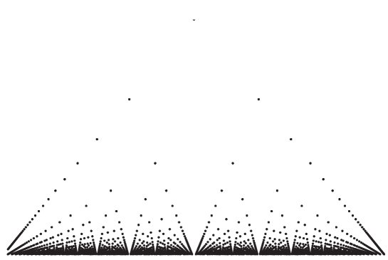
Figure 1: Popcorn (Thomae) function.

In order to demonstrate this fact accurately, consider some irrational number, $t$, at which $g(t)=0$, and take some $0<\varepsilon<1$. Without the loss of generality $\varepsilon$ is assumed to be rational, otherwise one may replace $\varepsilon$ with any smaller rational $\varepsilon^{\prime}=\frac{k}{m}<\varepsilon$ such that $\mathrm{gcd}(k,m)=1$. Thus, there is a finite set of the rational numbers $\Omega_{\varepsilon}=\{q=\frac{i}{j},1<j\leq m,1\leq i<j\}$, whose popcorn-values are not smaller than $g(\varepsilon)$. Now assign $\delta(\varepsilon)=inf\{|q-t|,q\in\Omega_{\varepsilon}\}$ that defines the vicinity of $t$, in which the values of $g$ are smaller than $\varepsilon$:

$$|t-y|<\delta(\varepsilon)\rightarrow|g(t)-g(y)|=|g(y)|<\varepsilon$$ (2)

These inequalities prove the continuity of of the popcorn function $g(x)$ at irrational values of $x$.

To our point of view, the popcorn function has not yet received decent attention among researchers, though its emergence in various physical problems seems impressive, as we demonstrate below. Apparently, the main difficulty deals with the discontinuity of $g(x)$ at every rational point, which often results in a problematic theoretical treatment and interpretation of results for the underlying physical system. Thus, a natural, physically justified ”continuous approximation” to the popcorn function is very demanded.

Here we provide such an approximation, showing the generality of the ”popcorn-like” distributions for a class of one-dimensional disordered systems. From the mathematical point of view, we demonstrate that the popcorn function can be constructed on the basis of the modular Dedekind function, $\eta(x+iy)$, when the imaginary part, $y$, of the modular parameter $z=x+iy$ tends to 0.

One of the most beautiful incarnations of the popcorn function arises in a so-called ”Euclid orchard” representation. Consider an orchard of trees of unit hights located at every point $(an,am)$ of the two-dimensional square lattice, where $n$ and $m$ are nonnegative integers defining the lattice, and $a$ is the lattice spacing, $a=1/\sqrt{2}$. Suppose we stay on the line $n=1-m$ between the points $A(0,a)$ and $B(a,0)$, and observe the orchard grown in the first quadrant along the rays emitted from the origin $(0,0)$ – see the Fig. 2.

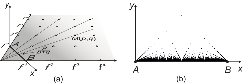
Figure 2: (a) Construction of the Euclid Orchard; (b) Thomae function.

Along these rays we see only the first open tree with coprime coordinates, $M(ap,aq)$, while all other trees are shadowed. Introduce the auxiliary coordinate basis $(x,y)$ with the axis $x$ along the segment $AB$ and $y$ normal to the orchard’s plane (as shown in the Fig. 2a). We set the origin of the $x$ axis at the point $A$, then the point $B$ has the coordinate $x=a$. It is a nice school geometric problem to establish that: (i) having the focus located at the origin, the tree at the point $M(ap,aq)$ is spotted at the place $x=\frac{p}{p+q}$, (ii) the visible height of this tree is $\frac{1}{p+q}$. In other words, the ”visibility diagram” of such a lattice orchard is exactly the popcorn function.

The popcorn correspondence $\frac{p}{q}\to\frac{1}{q}$ arises in the Euclid orchard problem as a purely geometrical result. However, the same function has appeared as a probability distribution in a plethora of biophysical and fundamental problems, such as the distribution of quotients of reads in DNA sequencing experiment dna , quantum $1/f$ noise and Frenel-Landau shift planat , interactions of non-relativistic ideal anyons with rational statistics parameter in the magnetic gauge approach lundholm , or frequency of specific subgraphs counting in the protein-protein network of a Drosophilla drosophilla . Though the extent of similarity with the original popcorn function could vary, and experimental profiles may drastically depend on peculiarities of each particular physical system, a general probabilistic scheme resulting in the popcorn-type manifestation of number-theoretic behavior in nature, definitely survives.

Suppose two random integers, $\phi$ and $\psi$, are taken independently from a discrete probability distribution, $Q_{n}=f^{n}$, where $f=1-\varepsilon>0$ is a ”damping factor”. If $\mathrm{gcd}(p,q)=1$, then the combination $\nu=\frac{\phi}{\phi+\psi}$ has the popcorn-like distribution $P(\nu)$ in the asymptotic limit $\varepsilon\ll 1$:

$$P\left(\nu=\frac{p}{p+q}\right)=\sum_{n=1}^{\infty}f^{n(p+q)}=\frac{(1-\varepsilon)^{p+q}}{1-(1-\varepsilon)^{p+q}}\approx\frac{1}{\varepsilon(p+q)}$$ (3)

The formal scheme above can be understood on the basis of the generalized Euclid orchard construction, if one considers a $(1+1)$-dimensional directed walker on the lattice (see Fig. 2a), who starts from the lattice origin and makes $\phi$ steps along one axis, followed by $\psi$ steps along the other axis. At every step the walker can die with the probability $\varepsilon=1-f$. Then, having an ensemble of such walkers, one arrives at the ”orchard of walkers”, i.e. for some point $\nu$ on the $x$ axis, a fraction of survived walkers, $P(\nu)$, is given exactly by the popcorn function.

In order to have a relevant physical picture, consider a toy model of diblock-copolymer polymerization. Without sticking to any specific polymerization mechanism, consider an ensemble of diblock-copolymers $AB$, polymerized independently from both ends in a cloud of monomers of relevant kind (we assume, only $A-A$ and $B-B$ links to be formed). Termination of polymerization is provided by specific ”radicals” of very small concentration, $\varepsilon$: when a radical is attached to the end (irrespectively, $A$ or $B$), it terminates the polymerization at this extremity forever. Given the environment of infinite capacity, one assigns the probability $f=1-\varepsilon$ to a monomer attachment at every elementary act of the polymerization. If $N_{A}$ and $N_{B}$ are molecular weights of the blocks $A$ and $B$, then the composition probability distribution in our ensemble, $P\left(\varphi=\frac{N_{A}}{N_{A}+N_{B}}\right)$, in the limit of small $\varepsilon\ll 1$ is ”ultrametric” (see avetisov for the definition of the ultrametricity) and is given by the popcorn function:

$$P\left(\varphi=\frac{p}{p+q}\right)\approx\frac{1}{\varepsilon(p+q)}\stackrel{{\scriptstyle def}}{{=}}\frac{1}{\varepsilon}g(\varphi)$$ (4)

In the polymerization process described above we have assumed identical independent probabilities for the monomers of sorts (”colors”) $A$ and $B$ to be attached at both chain ends. Since no preference is implied, one may look at this process as at a homopolymer (”colorless”) growth, taking place at two extremities. For this process we are interested in statistical characteristics of the resulting ensemble of the homopolymer chains. What would play the role of ”composition” in this case, or in other words, how should one understand the fraction of monomers attached at one end? As we show below, the answer is rather intriguing: the respective analogue of the probability distribution is the spectral density of the ensemble of linear chains with the probability $Q_{L}$ for the molecular mass distribution, where $L$ is the length of a chain in the ensemble.

II Spectral statistics of exponentially weighted ensemble of linear graphs

II.1 Spectral density and the popcorn function

The former exercises are deeply related to the spectral statistics of ensembles of linear polymers. In a practical setting, consider an ensemble of noninteracting linear chains with exponential distribution in their lengths. We claim the emergence of the fractal popcorn-like structure in the spectral density of corresponding adjacency matrices describing the connectivity of elementary units (monomers) in linear chains.

The ensemble of exponentially weighted homogeneous chains, is described by the bi-diagonal symmetric $N\times N$ adjacent matrix $B=\{b_{ij}\}$:

$$B=\left(\begin{array}[]{ccccc}0&x_{1}&0&0&\cdots\\ x_{1}&0&x_{2}&0&\\ 0&x_{2}&0&x_{3}&\\ 0&0&x_{3}&0&\\ \vdots&&&&\ddots\end{array}\right)$$ (5)

where the distribution of each $b_{i,i+1}=b_{i+1,i}=x_{i}$ ($i=1,...,N$) is Bernoullian:

$$x_{i}=\left\{\begin{array}[]{ll}1&\mbox{with probability $x$}\vskip 6.0pt plus 2.0pt minus 2.0pt\\ 0&\mbox{with probability $\varepsilon=1-f$}\end{array}\right.$$ (6)

We are interested in the spectral density, $\rho_{\varepsilon}(\lambda)$, of the ensemble of matrices $B$ in the limit $N\to\infty$. Note that at any $x_{k}=0$, the matrix $B$ splits into independent blocks. Every $n\times n$ block is a symmetric $n\times n$ bi-diagonal matrix $A_{n}$ with all $x_{k}=1$, $k=1,...,n$, which corresponds to a chain of length $n$. The spectrum of the matrix $A_{n}$ is

$$\lambda_{k,n}=2\cos\frac{\pi k}{n+1};\qquad(k=1,...,n)$$ (7)

All the eigenvalues $\lambda_{k,n}$ for $k=1,...,n-1$ appear with the probability $Q_{n}=f^{n}$ in the spectrum of the matrix (5). In the asymptotic limit $\varepsilon\ll 1$, one may deduce an equivalence between the composition distribution in the polymerization problem, discussed in the previous section, and the spectral density of the linear chain ensemble. Namely, the probability of a composition $\varphi=\frac{p}{p+q}$ in the ensemble of the diblock-copolymers can be precisely mapped onto the peak intensity (the degeneracy) of the eigenvalue $\lambda=\lambda_{p,p+q-1}=2\cos\frac{\pi p}{p+q}$ in the spectrum of the matrix $B$. In other words, the integer number $k$ in the mode $\lambda_{k,n}$ matches the number of $A$-monomers, $N_{A}=kz$, while the number of $B$-monomers matches $N_{B}=(n+1-k)z$, where $z\in N$, in the respective diblock-copolymer.

The spectral statistics survives if one replaces the ensemble of Bernoullian two-diagonal adjacency matrices $B$ defined by (5)–(6) by the ensemble of random Laplacian matrices. Recall that the Laplacian matrix, $L=\{a_{ij}\}$, can be constructed from adjacency matrix, $B=\{b_{ij}\}$, as follows: $a_{ij}=-b_{ij}$ for $i\neq j$, and $a_{ii}=\sum_{j=1}^{N}b_{ij}$. A search for eigenvalues of the Laplacian matrix $L$ for linear chain, is equivalent to determination its relaxation spectrum. Thus, the density of the relaxation spectrum of the ensemble of noninteracting linear chains with the exponential distribution in lengths, has the signature of the popcorn function.

To derive $\rho_{\varepsilon}(\lambda)$ for arbitrary values of $\varepsilon$, let us write down the spectral density of the ensemble of $N\times N$ random matrices $B$ with the bimodal distribution of the elements as a resolvent:

$$\rho_{\varepsilon}(\lambda)=\lim_{N\to\infty}\Big{<}\sum_{k=1}^{n}\delta(\lambda-\lambda_{kn})\Big{>}_{Q_{n}}=\lim_{N\to\infty\atop y\to+0}y\;\textrm{Im}\,\,\Big{<}G_{n}(\lambda-iy)\Big{>}_{Q_{n}}=\lim_{N\to\infty\atop y\to+0}y\sum_{n=1}^{N}Q_{n}\;\textrm{Im}\,\,G_{n}(\lambda-iy)$$ (8)

where $\left<...\right>_{Q_{n}}$ means averaging over the distribution $Q_{n}=(1-\varepsilon)^{n}$, and the following regularization of the Kronecker $\delta$-function is used:

$$\delta(\xi)=\lim_{y\to+0}\textrm{Im}\,\frac{y}{\xi-iy}$$ (9)

The function $G_{n}$ is associated with each particular gapless matrix $B$ of $n$ sequential ”1” on the sub-diagonals,

$$G_{n}(\lambda-iy)=\sum_{k=1}^{n}\frac{1}{\lambda-\lambda_{k,n}-iy}$$ (10)

Collecting (7), (8) and (10), we find an explicit expression for the density of eigenvalues:

$$\rho_{\varepsilon}(\lambda)=\lim_{N\to\infty\atop y\to+0}y\sum_{n=1}^{N}(1-\varepsilon)^{n}\sum_{k=1}^{n}\frac{y}{\left(\lambda-2\cos\frac{\pi k}{n+1}\right)^{2}+y^{2}}$$ (11)

The behavior of the inner sum in the spectral density in the asymptotic limit $y\to 0$ is easy to understand: it is $\frac{1}{y}$ at $\lambda=2\cos{\frac{\pi k}{n+1}}$ and zero otherwise. Thus, one can already infer a qualitative similarity with the popcorn function. It turns out, that the correspondence is quantitative for $\varepsilon=1-f\ll 1$. Driven by the purpose to show it, we calculate the values of $\rho_{\varepsilon}(\lambda)$ at the peaks, i.e. at rational points $\lambda=2\cos{\frac{\pi p}{p+q}}$ with $\mathrm{gcd}(p,q)=1$ and end up with the similar geometrical progression, as for the case of diblock-copolymers problem (3):

$$\rho_{\varepsilon}\left(\lambda=2\cos{\frac{\pi p}{p+q}}\right)=\sum_{s=1}^{\infty}(1-\varepsilon)^{(p+q)s-1}=\frac{(1-\varepsilon)^{p+q-1}}{1-(1-\varepsilon)^{p+q}}\Bigg{|}_{\varepsilon\to 0}\approx\frac{1}{\varepsilon(p+q)}\stackrel{{\scriptstyle def}}{{=}}g\left(\frac{1}{\pi}\arccos{\frac{\lambda}{2}}\right)$$ (12)

The typical sample plot $\rho_{\varepsilon}(\lambda)$ for $f=0.7$ computed numerically via (11) with $\varepsilon=2\times 10^{-3}$ is shown in the Fig. 3 for $N=10^{3}$.

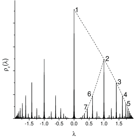
Figure 3: The spectral density $\rho_{\varepsilon}(\lambda)$ for the ensemble of bi-diagonal matrices of size $N=10^{3}$ at $f=0.7$. The regularization parameter $\varepsilon$ is taken $\varepsilon=2\times 10^{-3}$.

II.2 Enveloping curves and tails of the eigenvalues density

Below we pay attention to some number-theoretic properties of the spectral density of the argument $-\lambda$, since in this case the correspondence with the composition ratio is precise. One can compute the enveloping curves for any monotonic sequence of peaks depicted in Fig. 3, where we show two series of sequential peaks: $S_{1}=\{$1–2–3–4–5–…$\}$ and $S_{2}=\{$2–6–7–…$\}$. Any monotonic sequence of peaks corresponds to the set of eigenvalues $\lambda_{k,n}$ constructed on the basis of a Farey sequence farey . For example, as shown below, the peaks in the series $S_{1}$ are located at:

$$\lambda_{k}=-\lambda_{k,k}=-2\cos\frac{\pi k}{k+1},\qquad(k=1,2,...)$$

while the peaks in the series $S_{2}$ are located at:

$$\lambda_{k^{\prime}}=-\lambda_{k^{\prime},2k^{\prime}-2}=-2\cos\frac{\pi k^{\prime}}{2k^{\prime}-1},\qquad(k^{\prime}=2,3,...)$$

Positions of peaks obey the following rule: let $\{\lambda_{k-1},\,\lambda_{k},\,\lambda_{k+1}\}$ be three consecutive monotonically ordered peaks (e.g., peaks 2–3–4 in Fig. 3), and let

$$\lambda_{k-1}=-2\cos\frac{\pi p_{k-1}}{q_{k-1}},\quad\lambda_{k+1}=-2\cos\frac{\pi p_{k+1}}{q_{k+1}}$$

where $p_{k}$ and $q_{k}$ ($k=1,...,N$) are coprimes. The position of the intermediate peak, $\lambda_{k}$, is defined as

$$\lambda_{k}=-2\cos\frac{\pi p_{k}}{q_{k}};\qquad\frac{p_{k}}{q_{k}}=\frac{p_{k-1}}{q_{k-1}}\oplus\frac{p_{k+1}}{q_{k+1}}\equiv\frac{p_{k-1}+p_{k+1}}{q_{k-1}+q_{k+1}}$$ (13)

The sequences of coprime fractions constructed via the $\oplus$ addition are known as Farey sequences. A simple geometric model behind the Farey sequence, known as Ford circles ford ; coxeter , is shown in Fig. 4a. In brief, the construction goes as follows. Take the segment $[0,1]$ and draw two circles $O_{1}$ and $O_{2}$ both of radius $r=\frac{1}{2}$, which touch each other, and the segment at the points 0 and 1. Now inscribe a new circle $O_{3}$ touching $O_{1}$, $O_{2}$ and $[0,1]$. Where is the position of the new circle along the segment? The generic recursive algorithm constitutes the Farey sequence construction. Note that the same Farey sequence can be sequentially generated by fractional-linear transformations (reflections with respect to the arcs) of the fundamental domain of the modular group $SL(2,Z)$ – the triangle lying in the upper halfplane $\textrm{Im}\,z>0$ of the complex plane $z$ (see Fig. 4b).

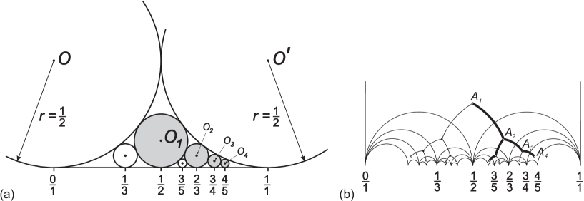
Figure 4: Ford circles as illustration of the Farey sequence construction: (a) Each circle touches two neighbors (right and left) and the segment. The position of newly generated circle is determined via the $\oplus$ addition: $\frac{p_{k-1}}{q_{k-1}}\oplus\frac{p_{k+1}}{q_{k+1}}=\frac{p_{k-1}+p_{k+1}}{q_{k-1}+q_{k+1}}$; (b) The same Farey sequence generated by sequential fractional-linear transformations of the fundamental domain of the modular group $SL(2,Z)$.

Consider the main peaks series, $S_{1}=\{$1–2–3–4–5–…$\}$. The explicit expression for their positions reads as:

$$\lambda_{k}=-2\cos\frac{\pi k}{k+1};\qquad k=1,2,...$$ (14)

One can straightforwardly investigate the asymptotic behavior of the popcorn function in the limit $k\to\infty$. From (12) one has for arbitrary $f<1$ the set of parametric equations:

$$\left\{\begin{array}[]{l}\displaystyle\rho_{\varepsilon}(\lambda_{k})=\frac{f^{k}}{1-f^{k+1}}\Big{|}_{k\gg 1}\approx f^{k}\\ \displaystyle\lambda_{k}=-2\cos\frac{\pi k}{k+1}\Big{|}_{k\gg 1}\approx 2-\frac{\pi^{2}}{k^{2}}\end{array}\right.$$ (15)

From the second equation of (15), we get $k\approx\frac{\pi}{\sqrt{2-\lambda}}$. Substituting this expression into the first one of (15), we end up with the following asymptotic behavior of the spectral density near the spectral edge $\lambda\to 2^{-}$:

$$\rho_{\varepsilon}(\lambda)\approx\exp\left(\frac{\pi\ln f}{\sqrt{2-\lambda}}\right)\qquad(0<f<1)$$ (16)

The behavior (15) is the signature of the Lifshitz tail typical for the 1D Anderson localization:

$$\rho_{\varepsilon}(E)\approx e^{-CE^{-D/2}};$$ (17)

where $E=2-\lambda$ and $D=1$.

III From popkorn to Dedekind $\eta$-function

III.1 Some facts about Dedekind $\eta$-function and related series

The popcorn function has discontinuous maxima at rational points and continuous valleys at irrationals. We show in this section, that the popcorn function can be regularized on the basis of the everywhere continuous Dedekind function $\eta(x+iy)$ in the asymptotic limit $y\to 0$.

The famous Dedekind $\eta$-function is defined as follows:

$$\eta(z)=e^{\pi iz/12}\prod_{n=0}^{\infty}(1-e^{2\pi inz})$$ (18)

The argument $z=x+iy$ is called the modular parameter and $\eta(z)$ is defined for $\textrm{Im}\,z>0$ only. The Dedekind $\eta$-function is invariant with respect to the action of the modular group $SL(2,\mathbb{Z})$:

$$\begin{array}[]{l}\eta(z+1)=e^{\pi iz/12}\;\eta(z)\vskip 6.0pt plus 2.0pt minus 2.0pt\\ \eta\left(-\frac{1}{z}\right)=\sqrt{-i}\;\eta(z)\end{array}$$ (19)

And, in general,

$$\eta\left(\frac{az+b}{cz+d}\right)=\omega(a,b,c,d)\;\sqrt{cz+d}\;\eta(z)$$ (20)

where $ad-bc=1$ and $\omega(a,b,c,d)$ is some root of 24th degree of unity dedekind .

It is convenient to introduce the following ”normalized” function

$$h(z)=|\eta(z)|(\textrm{Im}\,z)^{1/4}$$ (21)

The analytic structure of $h(z)$ has been discussed in avetisov in the context of the ultrametric landscape construction. In particular, the function $h(z)$ satisfies the duality relation, which follows from (19)–(20):

$$h\left(\left\{\frac{m}{k}\right\}+iy\right)=h\left(\left\{\frac{n}{k}\right\}+\frac{i}{k^{2}y}\right)$$ (22)

where $mn-kr=1,\;\{k,m,n,r\}\in\mathbb{Z},\;(y>0)$ and $\left\{\frac{m}{k}\right\},\left\{\frac{s}{k}\right\}$ denote fractional parts of corresponding quotients. In Appendix we use Eq.(22) to compute the values of $h(x+iy)$ at rational points $x$ near the real axis, i.e. at $y\to 0$.

The real analytic Eisenstein series $E(z,s)$ is defined in the upper half-plane, $H=\{z:\textrm{Im}\,(z)>0\}$ for $\textrm{Re}\,(s)>1$ as follows:

$$E(z,s)=\frac{1}{2}\sum_{\{m,n\}\in\mathbb{Z}^{2}\backslash\{0,0\}}\frac{y^{s}}{|mz+n|^{2s}};\qquad z=x+iy$$ (23)

This function can be analytically continued to all $s$-plane with one simple pole at $s=1$. Notably it shares the same invariance properties on $z$ as the Dedekind $\eta$-function. Moreover, $E(s,z)$, as function of $z$, is the $SL(2,\mathbb{Z})$–automorphic solution of the hyperbolic Laplace equation:

$$-y^{2}\left(\frac{\partial^{2}}{\partial x^{2}}+\frac{\partial^{2}}{\partial y^{2}}\right)E(z,s)=s(1-s)\;E(z,s)$$

The Eisenstein series is closely related to the Epstein $\zeta$-function, $\zeta(s,Q)$, namely:

$$\zeta(s,Q)=\sum_{\{m,n\}\in\mathbb{Z}^{2}\backslash\{0,0\}}\frac{1}{Q(m,n)^{s}}=\frac{2}{d^{s/2}}E(z,s),$$ (24)

where $Q(m,n)=am^{2}+2bmn+cn^{2}$ is a positive definite quadratic form, $d=ac-b^{2}>0$, and $\displaystyle z=\frac{-b+i\sqrt{d}}{a}$. Eventually, the logarithm of the Dedekind $\eta$-function is known to enter in the Laurent expansion of the Epstein $\zeta$-function. Its residue at $s=1$ has been calculated by Dirichlet and is known as the first Kronecker limit formula epstein ; siegel ; motohashi . Explicitly, it reads at $s\to 1$:

$$\zeta(s,Q)=\frac{\pi}{\sqrt{d}}\frac{1}{s-1}\\ +\frac{2\pi}{\sqrt{d}}\left(\gamma+\ln\sqrt{\frac{a}{4d}}-2\ln|\eta(z)|\right)+O(s-1)$$ (25)

Equation (25) establishes the important connection between the Dedekind $\eta$-function and the respective series, that we substantially exploit below.

III.2 Relation between the popcorn and Dedekind $\eta$ functions

Consider an arbitrary quadratic form $Q^{\prime}(m,n)$ with unit determinant. Since $d=1$, it can be written in new parameters $\{a,b,c\}\to\{x=\frac{b}{c},\varepsilon=\frac{1}{c}\}$ as follows:

$$Q^{\prime}(m,n)=\frac{1}{\varepsilon}(xm-n)^{2}+\varepsilon m^{2}$$ (26)

Applying the first Kronecker limit formula to the Epstein function with (26) and $s=1+\tau$, where $\tau\ll 1$, but finite one gets:

$$\zeta(s,Q^{\prime})=\frac{\pi}{s-1}+2\pi\left(\gamma+\ln\sqrt{\frac{1}{4\varepsilon}}-2\ln|\eta(x+i\varepsilon)|\right)+O(s-1)$$ (27)

On the other hand, one can make use of the $\varepsilon$-continuation of the Kronecker $\delta$-function, (9), and assess $\zeta(1+\tau,Q^{\prime})$ for small $\tau\ll 1$ as follows:

$$\zeta(1+\tau,Q^{\prime})\approx\frac{1}{\varepsilon}\sum_{\{m,n\}\in\mathbb{Z}^{2}\backslash\{0,0\}}\frac{\varepsilon^{2}}{\left(xm-n\right)^{2}+\varepsilon^{2}m^{2}}=\frac{2}{\varepsilon}\lim_{N\to\infty}\sum_{m=1}^{N}\sum_{n=1}^{N}\frac{1}{m^{2}}\delta\left(x-\frac{n}{m}\right)\equiv\theta(x);\qquad x\in(0,1)$$ (28)

where the factor 2 reflects the presence of two quadrants on the $\mathbb{Z}^{2}$-lattice that contribute jointly to the sum at every rational points, while $\theta$ assigns 0 to all irrationals. At rational points $\theta\left(\frac{p}{q}\right)$ can be calculated straightforwardly:

$$\theta\left(\frac{p}{q}\right)=\frac{2}{\varepsilon}\sum_{m|q}^{\infty}\frac{1}{m^{2}}=\frac{\pi^{2}}{3\varepsilon q^{2}}$$ (29)

Comparing (29) with the definition of the popcorn function, $g$, one ends up with the following relation at the peaks:

$$g\left(\frac{p}{q}\right)=\sqrt{\frac{3\varepsilon}{\pi^{2}}\theta\left(\frac{p}{q}\right)}$$ (30)

Eventually, collecting (27) and (30), we may write down the regularization of the popcorn function by the Dedekind $\eta(x+i\varepsilon)|_{\varepsilon\to 0}$ in the interval $0<x<1$:

$$g(x)\approx\sqrt{-\frac{12\varepsilon}{\pi}\ln|\eta(x+i\varepsilon)|-o\left(\varepsilon\ln\varepsilon\right)}\Bigg{|}_{\varepsilon\to 0}$$ (31)

or

$$-\ln|\eta(x+i\varepsilon)|_{\varepsilon\to 0}=\frac{\pi}{12\varepsilon}g^{2}(x)+O(\ln\varepsilon)$$ (32)

Note, that the asymptotic behavior of the Dedekind $\eta$-function can be independently derived through the duality relation, avetisov . However, such approach leaves in the dark the underlying structural equivalence of the popcorn and $\eta$ functions and their series representation on the lattice $\mathbb{Z}^{2}$. In the Fig. 5 we show two discrete plots of the left and the right-hand sides of (32).

Thus, the spectral density of ensemble of linear chains, (12), in the regime $\varepsilon\ll 1$ is expressed through the Dedekind $\eta$-function as follows:

$$\rho_{\varepsilon}(\lambda)\approx\sqrt{-\frac{12\varepsilon}{\pi}\ln\Bigg{|}\eta\left(\frac{1}{\pi}\arccos{\frac{\lambda}{2}}+i\varepsilon\right)\Bigg{|}}$$ (33)

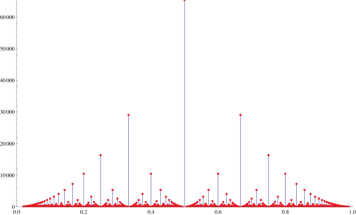
Figure 5: Plots of everywhere continuous $f_{1}(x)=-\ln|\eta(x+i\varepsilon)|$ (blue) and discrete $f_{2}(x)=\frac{\pi}{12\varepsilon}g^{2}(x)$ (red) for $\varepsilon=10^{-6}$ at rational points in $0<x<1$.

III.3 Continued Fractions and Invariant Measure

The behavior of the spectral density of our model is very similar to the one encountered in the study of harmonic chains with binary distribution of random masses. This problem, which goes back to F. Dyson dyson , has been investigated by C. Domb et al. in domb and then thoroughly discussed by T. Nieuwenhuizen and M. Luck in huisen . Namely, consider a harmonic chain of masses, which can take two values, $m$ and $M>m$:

$$\left\{\begin{array}[]{cl}m&\mbox{with the probability $1-f$}\vskip 6.0pt plus 2.0pt minus 2.0pt\\ M&\mbox{with the probability $f$}\end{array}\right.$$ (34)

In the limit $M\to\infty$ the system breaks into ”uniform harmonic islands”, each consisting of $n$ light masses (in what follows we take $m=1$ for simplicity) surrounded by two infinitely heavy masses. The probability of such an island is $(1-f)^{2}f^{n}$. There is a straightforward mapping of this system to the exponentially weighted ensemble of linear graphs discussed in the previous section.

Many results concerning the spectral statistics of ensemble of sequence of random composition of light and heavy masses were discussed in the works domb ; huisen . In particular, in huisen the integrated density of states, ${\cal N}(\lambda)$ has been written in the following form:

$${\cal N}(\lambda)=\int_{-\infty}^{\lambda}\rho(\lambda^{\prime})d\lambda^{\prime}=1-\frac{1-f}{f^{2}}\sum_{n=1}^{\infty}f^{\rm Int\left(\frac{n\pi}{\vartheta}\right)}$$ (35)

where the relation between $\lambda$ and $\vartheta$ is the following:

$$\cos\vartheta=\frac{\sqrt{\lambda+1}}{2}\qquad\left(0<\vartheta<\frac{\pi}{2}\right)$$ (36)

Note that (36) implies the asymmetry in the spectrum, $-1<\lambda<3$, that is related with presence of additional ”1” on the main diagonal of the adjacent matrix $B^{\prime}$, obtained from the matrix $B$ defined in (5). Both matrices are deeply related to the spectrum of resonance frequencies for the ensemble of linear chains with the distribution $Q_{n}$. Approximating the Laplacian by $O(h^{2})$-difference operator and rewriting the matrix eigenvalues problem as a boundary problem for a grid eigenfunction $y_{k}(i)$, corresponding to $\lambda_{k,n}$, one has:

$$\frac{y_{k}(i-1)-2y_{k}(i)+y_{k}(i+1)}{h^{2}}+w^{2}_{k,n}y_{k}(i)=0;\qquad 2\leq i\leq n-1$$ (37)

Since the frequencies $w^{2}_{k,n}$ are independent of the choice of the specific matrix ($B$ or $B^{\prime}$), being the characteristics of the ensemble, one may write down the relation between the eigenvalues $\lambda_{k,n}$ and $\lambda^{\prime}_{k,n}$:

$$\lambda_{k,n}=w^{2}_{k,n}+2;\qquad\lambda^{\prime}_{k,n}=w^{2}_{k,n}+3$$

Thus, the spectra of $B$ and $B^{\prime}$ are linked by the shift $\lambda^{\prime}_{k}=\lambda_{k}+1$ and spectrum of $B^{\prime}$ is asymmetric.

For $\lambda\to-1$ one gets ${\cal N}(\lambda)\to f/(1+f)$ which corresponds to the contribution of the states $\lambda=-1$ at the bottom of the spectrum. At the upper edge of the spectrum (for $\lambda\to 3^{-}$) one gets ${\cal N}(\lambda)\to 1$ which means that all states are counted. Equation (35) shows that the behavior near $\lambda=3$ (corresponding to $\vartheta=0$) is dominated by the first term ($n=1$) of the series. One has:

$${\cal N}(\lambda)\simeq 1-\frac{1-f}{f^{2}}\exp\left(\frac{2\pi\ln f}{\sqrt{3-\lambda}}\right)$$ (38)

The expression (38) signals the appearance of the Lifshitz singularity in the density of states. A more precise analysis shows that the tail (38) is modulated by a periodic function huisen .

Equation (35) displays many interesting features. In particular, the function ${\cal N}(\lambda)$ occurs in the mathematical literature as a generating function of the continued fraction expansion of $\displaystyle\frac{\pi}{\vartheta}$. Let us briefly sketch this connection following borwein . Consider the continued fraction expansion:

$$\frac{\pi}{\vartheta}=\frac{1}{\displaystyle c_{0}+\frac{1}{\displaystyle c_{1}+\frac{1}{\displaystyle c_{2}+\ldots}}}$$ (39)

where all $c_{n}$ are natural integers. Truncating this expansion at some level $n$, one gets a coprime quotient, $\frac{p_{n}}{q_{n}}$ which converges to $\frac{\pi}{\vartheta}$ when $n\to\infty$. A theorem of Borwein and Borwein borwein states that the generating function, $G(z)$ of the integer part of $\frac{\pi}{\vartheta}$

$$G(z)=\sum_{n=1}^{\infty}z^{\rm Int\left(\frac{n\pi}{\vartheta}\right)}$$

is given by the continued fraction expansion

$$G(z)=\frac{z}{1-z}\frac{1}{\displaystyle A_{0}+\frac{1}{\displaystyle A_{1}+\frac{1}{\displaystyle A_{2}+\ldots}}}$$

where

$$A_{n}(z)=\frac{z^{-q_{n}}-z^{-q_{n-2}}}{z^{-q_{n-1}}-1}$$

and $q_{n}$ is the denominator of the fraction $\frac{p_{n}}{q_{n}}$ approximating the value $\displaystyle\frac{\pi}{\vartheta}$. In order to connect $G(z)$ with the integrated density, (35), it is sufficient to set $z=f$ and express ${\cal N}(\lambda)$ in terms of $G(z)$. Then, from the equivalence discussed at the beginning of this section, the derivative of $N(\lambda)$ yields the popcorn function.

The connection between the popcorn function to the invariant measure has been discussed in different context in the work nechaev-comtet .

IV Conclusion

We have discussed the number-theoretic properties of distributions appearing in physical systems when an observable is a quotient of two independent exponentially weighted integers. The spectral density of ensemble of linear polymer chains distributed with the law $f^{L}$ ($0<f<1$), where $L$ is the chain length, serves as a particular example. In the sparse regime, namely at $f\to 1$, the spectral density can be expressed through the discontinuous and non-differentiable at all rational points, Thomae (”popcorn”) function. We suggest a continuous approximation of the popcorn function, based on the Dedekind $\eta$-function near the real axis.

Analysis of the spectrum at the edges reveals the Lifshitz tails, typical for the 1D Anderson localization. The non-trivial feature, related to the asymptotic behavior of the shape of the spectral density of the adjacency matrix, is as follows. The main, enveloping, sequence of peaks $1-2-3-4-5...$ in the Fig. 3 has the asymptotic behavior $\rho(\lambda)\sim q^{\pi/\sqrt{2-\lambda}}$ (at $\lambda\to 2^{-}$) typical for the 1D Anderson localization, however any internal subsequence of peaks, like $2-6-7-...$, has the behavior $\rho^{\prime}(\lambda)\sim q^{\pi/|\lambda-\lambda_{cr}|}$ (at $\lambda\to\lambda_{cr}$) which is reminiscent of the Anderson localization in 2D.

We would like to emphasize that the ultrametric structure of some collective observables, like the spectral density of ensemble of sparse random Schrödinger-like operators, is ultimately connected to number-theoretic properties of modular functions, like the Dedekind $\eta$-function, and demonstrate the hidden $SL(2,Z)$ modular symmetry. We also pay attention to the connection of the Dedekind $\eta$-function near the real axis to the invariant measures of some continued fractions studied by Borwein and Borwein in 1993 borwein .

The notion of ultrametricity deals with the concept of hierarchical organization of energy landscapes mez ; fra . A complex system is assumed to have a large number of metastable states corresponding to local minima in the potential energy landscape. With respect to the transition rates, the minima are suggested to be clustered in hierarchically nested basins, i.e. larger basins consist of smaller basins, each of these consists of even smaller ones, etc. The basins of local energy minima are separated by a hierarchically arranged set of barriers: large basins are separated by high barriers, and smaller basins within each larger one are separated by lower barriers. Ultrametric geometry fixes taxonomic (i.e. hierarchical) tree-like relationships between elements and, speaking figuratively, is closer to Lobachevsky geometry, rather to the Euclidean one.

Appendix A Asymptotics of $\eta(x+iy)$ at rational $x$ and $y\to 0$

Here we shall obtain the asymptotics of $\eta(z)$ at $y\to 0^{+}$. Take into account the relation of the Dedekind $\eta$ with Jacobi elliptic functions:

$$\vartheta_{1}^{\prime}(0,e^{\pi iz})=\eta^{3}(z)$$ (40)

where

$$\vartheta_{1}^{\prime}(0,e^{\pi iz})\equiv\frac{d\vartheta_{1}(u,e^{\pi iz})}{du}\bigg{|}_{u=0}=e^{\pi iz/4}\sum_{j=0}^{\infty}(-1)^{j}(2j+1)e^{i\pi j(j+1)z}$$ (41)

Rewrite (22) in terms of $\eta$-functions:

$$\left|\eta\left(\left\{\frac{m}{k}\right\}+iy\right)\right|=\frac{1}{\sqrt{ky}}\left|\eta\left(\left\{\frac{n}{k}\right\}+\frac{i}{k^{2}y}\right)\right|$$ (42)

Applying (40)–(41) to (42), we get:

$$\left|\eta\left(\left\{\frac{m}{k}\right\}+iy\right)\right|=\frac{1}{\sqrt{ky}}\left|e^{\frac{\pi}{4}i\left(\left\{\frac{n}{k}\right\}+\frac{i}{k^{2}y}\right)}\sum_{j=0}^{\infty}(-1)^{j}(2j+1)e^{i\pi j(j+1)\left(\left\{\frac{n}{k}\right\}+\frac{i}{k^{2}y}\right)}\right|^{1/3}$$ (43)

Equation (43) enables us to extract the leading asymptotics of $\left|\eta\left(\left\{\frac{m}{k}\right\}+iy\right)\right|$ in the $y\to 0^{+}$ limit. Note that every term in the series in (43) for any $n\geq 1$ and for small $y$ (i.e. for $y\ll k^{-2}$) converges exponentially fast, we have

$$\left|\eta\left(\left\{\frac{m}{k}\right\}+iy\right)\right|_{y\to 0^{+}}\to\frac{1}{\sqrt{ky}}e^{-\frac{\pi}{12k^{2}y}};$$ (44)

Thus, we have finally:

$$\sqrt{-\ln\left|\eta\left(\left\{\frac{m}{k}\right\}+iy\right)\right|}\Bigg{|}_{y\to 0^{+}}\to\frac{1}{k}\sqrt{\frac{\pi}{12y}}$$ (45)

In (45) we have dropped out the subleading terms at $y\to 0^{+}$, which are of order of $O(\ln y)$.

References

- (1) Beanland, K., Roberts, J. W., Stevenson, C., Modifications of Thomae’s function and differentiability. American Mathematical Monthly, 116 531 (2009).
- (2) Trifonov, V., Pasqualucci, L., Dalla-Favera, R., Rabadan, R., Fractal-like distributions over the rational numbers in high-throughput biological and clinical data, Scientific reports, 1 191 (2011).
- (3) Planat, M., Eckert, C., On the frequency and amplitude spectrum and the fluctuations at the output of a communication receiver, IEEE transactions on ultrasonics, ferroelectrics, and frequency control, 47 1173 (2000)
- (4) Lundholm, D. (2016). Many-anyon trial states, ArXiv:1608.05067.
- (5) Middendorf, M., Ziv, E., Wiggins, C. H., Inferring network mechanisms: the Drosophila melanogaster protein interaction network, PNAS, 102 3192 (2005).
- (6) Avetisov, V., Krapivsky, P. L., Nechaev, S. (2015). Native ultrametricity of sparse random ensembles, Journal of Physics A: Mathematical and Theoretical, 49 035101 (2015).
- (7) Hardy, G. H., Wright, E. M., An introduction to the theory of numbers, Oxford University Press, 1979.
- (8) Ford, L. R. (1938). Fractions, Am. Math. Monthly, 45 586 (1938).
- (9) Coxeter, H. S. M., The problem of Apollonius, Am. Math. Monthly, 75, 5 (1968).
- (10) Chandrassekharan, K., Elliptic Functions, Berlin: Springer, 1985.
- (11) Epstein, P., Zur Theorie allgemeiner Zetafunctionen. Mathematische Annalen, 56 615 (1903).
- (12) Siegel, C. L., Lectures on advanced analytic number theory, Tata Inst. of Fund. Res., Bombay, 1961.
- (13) Motohashi, Y.,A new proof of the limit formula of Kronecker, Proceedings of the Japan Academy, 44, 614 (1968).
- (14) Dyson, F. J., The dynamics of a disordered linear chain, Physical Review, 92 1331 (1953)
- (15) Domb, C., Maradudin, A. A., Montroll, E. W., Weiss, G. H., Vibration Frequency Spectra of Disordered Lattices. I. Moments of the Spectra for Disordered Linear Chains, Physical Review, 115 18 (1959).
- (16) Nieuwenhuizen, T. M., Luck, J. M., Singular behavior of the density of states and the Lyapunov coefficient in binary random harmonic chains, J. Stat. Phys., 41, 745 (1985).
- (17) Borwein, J. M., Borwein, P. B., On the generating function of the integer part:, Journal of Number Theory, 43, 293 (1993).
- (18) Comtet, A., Nechaev, S., Random operator approach for word enumeration in braid groups, Journal of Physics A: Mathematical and General, 31, 5609 (1998).
- (19) Mezard, M., Parisi, G., Virasoro, M., Spin glass theory and beyond: An Introduction to the Replica Method and Its Applications (Vol. 9), WSPC, 1987.
- (20) Frauenfelder, H. (1987), The connection between low-temperature kinetics and life. In Protein Structure (pp. 245-261). Springer: New York, 1987.