Smooth Interpolation of Key Frames in a Riemannian Shell Space

Abstract

Splines and subdivision curves are flexible tools in the design and manipulation of curves in Euclidean space. In this paper we study generalizations of interpolating splines and subdivision schemes to the Riemannian manifold of shell surfaces in which the associated metric measures both bending and membrane distortion. The shells under consideration are assumed to be represented by Loop subdivision surfaces. This enables the animation of shells via the smooth interpolation of a given set of key frame control meshes. Using a variational time discretization of geodesics efficient numerical implementations can be derived. These are based on a discrete geodesic interpolation, discrete geometric logarithm, discrete exponential map, and discrete parallel transport. With these building blocks at hand discrete Riemannian cardinal splines and three different types of discrete, interpolatory subdivision schemes are defined. Numerical results for two different subdivision shell models underline the potential of this approach in key frame animation.

Keywords cardinal splines, interpolatory subdivision, Riemannian calculus, shape space, exponential map, logarithm, variational discretization

MSC(2010) 68U07, 65D05, 65D17, 49M25

1 Introduction

In this paper we investigate classical interpolation and approximation tools for curves in the context of Riemannian manifolds and specifically a shape manifold of subdivision shell surfaces. To this end we pick up the time-discrete geodesic calculus developed by Rumpf and Wirth in [53] and applied to shell space by Heeren et al. in [34, 32], and ask for effective and efficient generalizations of the de Casteljau algorithm for Bézier curves, cardinal splines, and several interpolatory subdivision schemes.

Recently, Riemannian calculus on shape spaces and in particular on the space of surfaces has attracted a lot of attention. Kilian et al. [41] studied geodesics in the space of triangular surfaces to interpolate between two given poses. The underlying metric is derived from the in-plane membrane distortion. Since this pioneering paper a variety of other Riemannian metrics on the space of surfaces have been investigated [44, 42, 43, 5, 37, 4, 7, 2]. In [34, 32] a metric was proposed that takes the full elastic responses including bending distortion into account. We pick up this metric and the associated variational discretization, which are briefly revisited below. Also based on this metric, Brandt et al. [6] proposed an accelerated scheme for the computation of geodesic paths in shell space. To this end they applied dimension reduction with respect to the surface models. Winkler et al. [63] and Fröhlich and Botsch [26] considered a representation of triangular meshes via a vector of edge lengths and dihedral angles and applied a back projection onto the space of triangular surfaces. This approach has been used by Heeren et al in [33] to simplify the computation of Riemannian splines in the space of images. For the smooth interpolation of given key frames and independent from the Riemannian concept, spacetime constraints were used by Witkin and Kass [64] to compute optimal trajectories. Smooth interpolating paths in high dimensional shape spaces have been investigated via a spacetime constraint approach as generalizations of traditional cubic B-splines by Kass and Anderson named wiggly splines [39]. These splines lack the theoretical foundation of an underlying Riemannian shape manifold. Another alternative approach is the animation approach by Schulz et al. [54, 55], which combines the wiggly spline method, suitable vibration modes and a new warping scheme. A discrete Riemannian approach for the smoothing of curves in a shape space of triangular meshes has been proposed by Brandt et al. [6]. They apply a gradient descent scheme for a discrete path energy on shell space picking up the the concept of the discrete path energy introduced in [34].

In Euclidean space cubic splines minimize the total squared second derivative. Analogously, Riemannian cubic splines were introduced by Noakes et al. [46] in a variational setting on Riemannian manifolds as smooth curves that are stationary paths of the integrated squared covariant derivative of the velocity. Subsequently, Camarinha et al. [8] proved a local optimality condition of this functional at a critical point and Giambo and Giannoni [27] established a global existence results. A typical application of this kind of higher-order interpolation is for instance path planning as it occurs naturally in aerospace and manufacturing industries. The associated Euler-Lagrange equation is a fourth-order differential equation, first derived in Noakes et al. [46] and then in Crouch and Silva Leite [16] in the context of dynamic interpolation. Crouch and Silva Leite also considered the interpolation problem for multiple points on a manifold. More recently, Trouvé and Vialard [58] developed a spline interpolation method on Riemannian manifolds and applied it to time-indexed sequences of 2D or 3D shapes where they focused on the finite dimensional case of landmarks. They introduced a control variable $u$ on the Hamiltonian equations of the geodesics. Hinkle et al. [35] introduced a family of higher order Riemannian polynomials to perform polynomial regression on Riemannian manifolds. They apply their approach to low dimensional embedded manifolds (e.g. the $d$-dimensional sphere), to the Lie group $SO(3)$ as well as shape spaces of 2D image data represented by landmark positions. In [33] a variational discretization of splines on shell space was presented. Thereby, discrete splines are defined as minimizers of the time discrete spline energy coupled with a set of variational constraints. Compared to the approach considered here, this method leads to a globally coupled system of all shells along a discrete curve in shell space, which is computationally challenging.

Different from these methods based on the intrinsic formulation using the covariant derivative on curves, extrinsic variational formulations have been studied, which minimize curve energies in ambient space where the restriction of the curve to the manifold is realized as a constraint. Wallner [59] showed existence of minimizers in this setup for finite dimensional manifolds, and Pottmann and Hofer [50] proved that these minimizers are $C^{2}$. In [36] they already provided a method for the computation of splines on parametric surfaces, level sets, triangle meshes and point set surfaces. Algorithmically, they alternately compute minimizers of the objective functional in the tangent plane and project back to the manifold. Our approach can not be formulated extrinsically, because the metric on shell space does not arise from an ambient Euclidean metric.

The concept of Bézier curves can easily be transferred to Riemannian manifolds and in particular to shape spaces. To this end the de Casteljau algorithm with linear interpolation has to be replaced by geodesic interpolation [49, 28, 1], compare also Effland et al. [23] for a corresponding tool on the shape space of images and Brandt et al. [6] for this method on the space of triangular shell surfaces using the variational time discretization [34]. Below we will discuss the de Casteljau algorithm on the space of subdivision surfaces to prepare the discussion of Hermite interpolation and cardinal splines.

In addition to variational formulations there are various approaches for interpolatory subdivision schemes on manifolds. These methods exploit the fact that subdivision schemes for curves in linear spaces are mostly based on repeated local averages. Dyn [21] proposed a Riemannian extension, where affine averaging is replaced by geodesic averaging. Wallner and Dyn [62] showed that the Riemannian extension of cubic subdivision yields $C^{1}$ curves. Their analysis is based on a comparison of subdivision schemes in Euclidean space—where $C^{1}$ smoothness results are obtained by studying the convergence of the symbol associated with the linear subdivision rule—and the corresponding scheme on a Riemannian manifold. Under a suitable proximity condition $C^{1}$ smoothness can be established. In [60] this technique is generalized to show higher smoothness and specifically for Lie groups $C^{2}$ smoothness of Riemannian subdivision schemes. More general proximity conditions which imply higher smoothness of the Riemannian counterpart of an linear subdivision scheme are analysed by Grohs in [31]. Dyn et al. show in [22] that the approximation order of nonlinear univariate schemes derived as perturbations of linear schemes is directly linked to the smoothness of the nonlinear scheme. In [20] Duchamp et al. studied higher order smoothness of manifold valued subdivision curves using a retraction map in the construction of the subdivision scheme. This retraction map is required to be a third-order approximation of the exponential map. Recently, Wallner [61] proved convergence of the linear four-point scheme and other univariate interpolatory schemes in Riemannian manifolds. To this end he studies Riemannian edge length contractivity of the schemes on a manifold combined with a multiresolutional analysis. In our case, concerning the consistency, there is not only the transfer of linear subdivision schemes to curved spaces. But there is also a second source of proximity errors, which is the approximation of the local squared Riemannian distance by a functional which is cheaper to compute. At the moment the convergence of the schemes considered here for fixed time step size is open. We refer to Section 6 for some comments in this direction.

We consider here Loop’s subdivision also for the representation of our shell surfaces. They are subdivision limit surfaces for given control meshes. Subdivision schemes for the modeling of geometries are widespread in geometry processing and computer graphics. For a comprehensive introduction to subdivision methods in general we refer the reader to [47] and [9]. Among the most popular subdivision schemes are the Catmull-Clark [10] and Doo-Sabin [19] schemes on quadrilateral meshes, and Loop’s scheme on triangular meshes [45]. The Loop subdivision basis functions have been extensively studied, in particular regarding their smoothness [51], curvature integrability [52], (local) linear independence [48, 65], approximation power [3], and robust evaluation around extraordinary vertices [56]. With respect to the use of subdivision methods in animation see [17, 57]. Nowadays, subdivision finite elements are also extensively used in engineering [14, 12, 15, 13, 30, 29].

Our contribution

In this paper we use recent progress on the theory of splines on Riemannian manifolds and take into account the Riemannian model of the space of shells proposed by Heeren et al. [34]. We show that various Euclidean concepts of interpolating curves can easily be transferred to the Riemannian shell space. To this end we slightly generalize the discrete geodesic calculus developed in [34] and [32] which allows for an elegant and robust implementation of a versatile toolbox for key frame interpolation. In detail our contributions are

• the generalization of discrete geodesics and the discrete exponential map introduced in [34] and [32] to points in time which are not multiples of a given time step size as an essential ingredient for the construction of smooth interpolating curves,

• a discrete Riemannian Catmull-Rom interpolation based on discrete Bézier curves and discrete parallel transport,

• different discrete Riemannian interpolatory subdivision schemes,

• and the conforming implementation of the geodesic calculus on the space of shells represented by subdivision surfaces including the new interpolation curves.

The organization of the paper is as follows. In Section 2 we recall some basic facts of Riemannian calculus and discuss the variational time discretization and the set up in the case of the space of shells represented by Loop subdivision surfaces. Section 3 is devoted to the review of discrete Bézier curves in shell space, whereas in Section 4 we derive discrete cardinal splines. Then in Section 5 different discrete interpolatory subdivision schemes are presented. Finally, in Section 6 we draw conclusions.

2 Variational time discretization of geodesic calculus in shell space

In this section we review the variational time discretization of geodesic calculus developed in [53] by Rumpf and Wirth and applied to a space of discrete shells by Heeren et al. in [34, 32]. This calculus includes in particular the notions of discrete geodesics, discrete logarithm, discrete exponential map, and discrete parallel transport. For results on existence and uniqueness of the associated geometric operators and the convergence to their continuous counterparts on finite dimensional Riemannian manifolds and certain infinite dimensional Hilbert manifolds we refer to [53].

Geodesic calculus on Riemannian manifolds

Let us denote by $(\mathcal{S},\,g)$ a smooth, complete Riemannian manifold with metric $g$. In our context $\mathcal{S}$ is a space of discrete shells and more specifically the space of shells represented by Loop subdivision surfaces. For a smooth path $(s(t))_{t\in[0,1]}$, the path length is defined by

$$\mathcal{L}[(s(t))_{t\in[0,1]}]=\int_{0}^{1}\sqrt{g_{s(t)}(\dot{s}(t),\dot{s}(t))}\,dt,$$ (1)

where $\dot{s}(t)\in T_{s(t)}\mathcal{S}$ denotes the velocity at time $t$. Given two shells $s_{A},s_{B}\in\mathcal{S}$, the minimizing path $(s(t))_{t\in[0,1]}$ of (1) is called shortest geodesic and the minimal path length defines the Riemannian distance $\mathrm{dist}(s_{A},s_{B})$ between $s_{A}$ and $s_{B}$. Geodesic paths also minimize the path energy

$$\mathcal{E}[(s(t))_{t\in[0,1]}]=\int_{0}^{1}g_{s(t)}(\dot{s}(t),\dot{s}(t))\,dt,$$ (2)

if in addition the speed $\sqrt{g_{s(t)}(\dot{s}(t),\dot{s}(t))}$ is constant. For small Riemannian distances shortest geodesics are unique. Then the geodesic averaging for $0\leq t\leq 1$ is given by

$$\mathcal{Av}(s_{A},s_{B},t)=s(t)$$ (3)

where $s(t)$ is assumed to be the shortest geodesic connecting $s_{A}$ and $s_{B}$. The exponential map is defined by

$$\exp_{s_{A}}(v)=s(1)\,,$$

where $t\mapsto s(t)$ is the solution of the Euler-Lagrange equation $\nabla_{\dot{s}(t)}\dot{s}(t)=0$ associated with the path energy for given $s(0)=s_{A}$ and $\dot{s}(0)=v\in T_{s_{A}}\mathcal{S}$. Here $\nabla_{\dot{s}(t)}$ denotes the covariant derivative along the geodesic. For sufficiently small $r$ the exponential map $\exp_{s_{A}}$ is a bijection from $B_{r}(0)\to\exp_{s_{A}}(B_{r}(0))$. For $s_{B}\in\exp_{s_{A}}(B_{r}(0))$ the inverse of $\exp_{s_{A}}$ defines the logarithm map

$$\log_{s_{A}}(s_{B})=v,$$

where $v$ is the initial velocity $\dot{s}(0)$ of the unique shortest geodesic connecting $s_{A}$ with $s_{B}$. Finally, the parallel transport of a given vector $w$ along a path $(s(t))_{t\in[0,1]}$ (not necessarily geodesic) is defined as

$${\mathrm{P}}_{(s(t))_{t\in[0,1]}}(w)=w(1)\,,$$

where $t\to w(t)$ solves $\nabla_{\dot{s}(t)}w(t)=0$ with initial data $w(0)=w$. For a detailed discussion we refer to [18].

Subdivision shell space

For the manifold $\mathcal{S}$ of discrete shells investigated in this paper an element of this space is a Loop subdivision surface described by a triangular control mesh $s$. Thus for fixed topology of the control mesh and a point to point correspondence of control meshes in $\mathcal{S}$ a discrete shell can be identified with a vector in $\mathbb{R}^{3M}$, where $M$ is the number of vertices of the control mesh. Physically, a subdivision surface with control mesh $s$ can be considered as the mid-surface of a thin, curved three-dimensional volumetric object whose thickness $\delta$ is relatively small compared to the area of the mid-surface. The associated metric reflects viscous dissipation in this thin surface layer when undergoing a deformation. To derive the metric we apply Rayleigh’s paradigm (cf. [34]), i.e. we start with a model for the elastic deformation of the thin layer and replace then strain by strain rates for a second order approximation of the energy.

To this end, we consider at first an elastic deformation $\phi$ of the homogeneous, isotropic material layer and approximate the energy by an elastic energy associated to the deformation of the midsurface split into a membrane and bending contribution; i.e. we define

$$Q_{{\mbox{{\tiny mem}}}}[\phi] =B^{{\mbox{{\tiny mem}}}}_{\phi}-B^{{\mbox{{\tiny mem}}}}_{{\mathds{1}}}\quad\text{and}\quad Q_{{\mbox{{\tiny bend}}}}[\phi]=B^{{\mbox{{\tiny bend}}}}_{\phi}-B^{{\mbox{{\tiny bend}}}}_{{\mathds{1}}}$$

with the symmetric operators $B^{{\mbox{{\tiny mem}}}}$ and $B^{{\mbox{{\tiny bend}}}}$ given by

$$\operatorname{{I}}_{s}(B^{{\mbox{{\tiny mem}}}}_{\phi}v,w) =\operatorname{{I}}_{\phi(s)}({\,\mathrm{d}}\phi(v),{\,\mathrm{d}}\phi(w))\,,$$

$$\operatorname{{I}}_{s}(B^{{\mbox{{\tiny bend}}}}_{\phi}v,w) =\operatorname{{II}}_{\phi(s)}({\,\mathrm{d}}\phi(v),{\,\mathrm{d}}\phi(w))\,.$$

Here, $\operatorname{{I}}_{s}$, $\operatorname{{II}}_{s}$ denote the first and second fundamental form with tangent vectors $v$ and $w$. In fact, $B^{{\mbox{{\tiny mem}}}}_{\phi}$ is the geometric (tangential) Cauchy-Green strain tensor for the deformation $\phi$ on the surface $s$ and $Q_{{\mbox{{\tiny bend}}}}[\phi]$ is the relative shape operator quantifying properly the difference in curvature between the deformed and the undeformed configuration. The total elastic deformation energy is then given by

$$\mathcal{W}_{s}^{D}[\phi]=\delta\int_{s}W_{{\mbox{{\tiny mem}}}}(Q_{{\mbox{{\tiny mem}}}}[\phi])\,{\,\mathrm{d}}x+\delta^{3}\int_{s}W_{{\mbox{{\tiny bend}}}}(Q_{{\mbox{{\tiny bend}}}}[\phi])\,{\,\mathrm{d}}x\ ,$$ (4)

where the non-negative energy densities $W_{{\mbox{{\tiny mem}}}}$ and $W_{{\mbox{{\tiny bend}}}}$ act on the symmetric linear rank two operators $Q_{{\mbox{{\tiny mem}}}}$ and $Q_{{\mbox{{\tiny bend}}}}$, respectively. For $W_{{\mbox{{\tiny mem}}}}$ and $W_{{\mbox{{\tiny bend}}}}$ we require that (i) $W(0)=0$, (ii) $DW=0$ at the zero matrix, and (iii) $D^{2}W$ is positive definite at the zero matrix. These requirements ensure that for a shell in a stress free configuration the deformation identity ${\mathds{1}}$ is a minimizer of $\mathcal{W}$ and thus (i) $\mathcal{W}_{s}^{D}[{\mathds{1}}]=0$ and (ii) $d\mathcal{W}_{s}^{D}[{\mathds{1}}]=0$. Additionally, we assume (iii) that the energy is strictly convex (modulo rigid body motions) in a neighborhood of a minimizer. These conditions capture most thin elastic materials [11]. Under these assumptions the application of Rayleigh’s paradigm indeed leads to a Riemannian metric as pointed out by Heeren et al. [32]. They showed the following result :
For $v$ a tangent vector field to a shell $s$ in the space of smooth shells $\mathcal{S}$, $\operatorname{{Hess}}(\mathcal{W}_{s}^{D})(v,v)=0$ if and only if $v$ induces an infinitesimal rigid motion. Consequently, $g_{s}(v,w)=\frac{1}{2}\operatorname{{Hess}}(\mathcal{W}_{s}^{D})(v,w)$ is indeed a Riemannian metric on the space of smooth shells modulo infinitesimal rigid body motions.
For the proof we refer to [32]. In the application, we consider the membrane energy density as suggested in [34]:

$$W_{{\mbox{{\tiny mem}}}}(Q) =\frac{\mu}{2}\mathrm{tr}Q+\frac{\lambda}{4}\det Q-\frac{2\mu+\lambda}{4}\log\det Q-\mu-\frac{\lambda}{4}.$$ (5)

Here, $\lambda$ and $\mu$ are the Lamé constants of linearized elasticity and $\mathrm{tr}$ and $\det$ denote the trace and the determinant, respectively, where $\det Q$ describes area distortion, while $\mathrm{tr}Q$ measures length distortion. The function $W_{{\mbox{{\tiny mem}}}}[Q]$ is rigid body motion invariant and the identity as deformation is the minimizer. Furthermore, the Hessian of the resulting path energy coincides with the quadratic form of linearized elasticity. The $\log\det Q$ term penalizes material compression. For the bending energy density we select the squared Frobenius norm of the embedded relative Weingarten map

$$W_{\mbox{{\tiny bend}}}(Q)=\mathrm{tr}(Q^{T}Q)\,.$$ (6)

Time-discrete geodesic calculus

To derive a variational discretization of the geodesic calculus we consider an approximation of the squared Riemannian distance $\mathrm{dist}^{2}$ by a smooth functional $\mathcal{W}:\mathcal{S}\times\mathcal{S}\to\mathbb{R}$, where we assume $s,\tilde{s}\in\mathcal{S}$:

$$\mathrm{dist}^{2}(s,\tilde{s})=\mathcal{W}[s,\tilde{s}]+\mathrm{dist}^{3}(s,\tilde{s}).$$ (7)

For a detailed discussion of this approximation we refer to [34]. For $g_{s}=\frac{1}{2}\mathcal{W}_{,22}[s,s]$ this assumption on $\mathcal{W}$ holds by Taylor expansion. In the case of the subdivision shell space introduced above, $\mathcal{W}[s,\tilde{s}]:=\mathcal{W}_{s}^{D}[\tilde{s}-s]$ fulfills the assumption with $\tilde{s}-s$ representing the deformation of $s$ to $\tilde{s}$ as a vector-valued subdivision function on $s$. Using the Cauchy-Schwarz inequality one obtains that $\mathcal{E}[(s(t))_{t\in[0,1]}]\geq\sum_{k=1}^{K}\mathrm{dist}(s(\frac{k-1}{K}),s(\frac{k}{K}))^{2}$, where equality holds only if $(s(t))_{t\in[0,1]}$ is already a shortest geodesic. This motivates the definition of the discrete path energy

$$\mathbf{E}[(s_{0},\ldots,s_{K})]=K\sum_{k=1}^{K}\mathcal{W}[s_{k-1},s_{k}]$$ (8)

of a discrete path $(s_{0},\ldots,s_{K})$. For given input shells $s_{A}$ and $s_{B}$ in $\mathcal{S}$ we call the discrete path $(s_{0},\ldots,s_{K})$ a discrete shortest geodesic, if $(s_{0}=s_{A},\ldots,s_{K}=s_{B})$ is a minimizer of the discrete path energy (8). The corresponding system of Euler–Lagrange equations is given by

$$\mathcal{W}_{,2}[s_{k-1},s_{k}]+\mathcal{W}_{,1}[s_{k},s_{k+1}]=0$$ (9)

for $k=1,\ldots,K-1$, where $\mathcal{W}_{,i}$ denotes the variation with respect to the $i$th argument. Then the discrete geodesic averaging for $0\leq k\leq K$ is defined by

$$\mathbf{Av}^{K}(s_{A},s_{B},k/K)=s_{k}$$ (10)

if $(s_{0},\ldots,s_{k},\ldots,s_{K})$ is the shortest discrete geodesic connecting $s_{0}=s_{A}$, $s_{K}=s_{B}$. Given a continuous geodesic $(s(t))_{t\in[0,1]}$ with $s(0)=s_{A}$ and $s(1)=s_{B}$ and a discrete geodesic $(s_{0},\ldots,s_{K})$ with $s_{0}=s_{A}$ and $s_{K}=s_{B}$, we may view $s_{1}-s_{0}$ as the discrete counterpart to $\tau\dot{s}(0)$ for $\tau=\frac{1}{K}$. Motivated by the fact that $\frac{1}{K}\;\log_{s_{A}}(s_{B})=\frac{1}{K}\dot{s}(0)$ we hence give the following definition of a discrete logarithm. Suppose we have a unique discrete geodesic $(s_{0}=s_{A},\ldots,s_{K}=s_{B})$, then we define the discrete logarithm by

$${\mathbf{Log}}^{K}_{s_{A}}(s_{B})=K(s_{1}-s_{0})\,.$$

As in the continuous case, the discrete logarithm can be considered as the linear representation of the nonlinear variation $s_{B}$ to $s_{A}$.

Next, we ask for fixed $s_{0}=s_{A}$ and $s_{1}=s_{A}+\tfrac{\xi}{K}$ for a solution $s_{2}$ of the Euler-Lagrange equation (9) for $K=2$: $0=\mathcal{W}_{,2}[s_{0},s_{1}]+\mathcal{W}_{,1}[s_{1},s_{2}]\,.$ One can show (cf. [53]) that for $s_{1}-s_{0}$ sufficiently small a unique solution $s_{2}$ exists and thus $(s_{0},s_{1},s_{2})$ is a discrete geodesic. Iterating this procedure, we compute for given $s_{k-1}$ and $s_{k}$ a solution $s_{k+1}$ of the equation (9) and obtain a variational scheme for the shooting of a discrete geodesics $(s_{0},\ldots,s_{k},\ldots)$. Thereby, $s_{k}$ is a discrete counter part of $\exp_{s_{A}}\left(\tfrac{k}{K}\xi\right)$ with $\tau=\tfrac{1}{K}$ being the time step size of the scheme. Hence, we introduce the discrete exponential map

$$\mathbf{Exp}^{K}_{s_{A}}(\tfrac{k}{K},\xi)=s_{k}\,.$$

Let us emphasize that we use here a slightly different notation as to [53] with a more natural scaling of arguments and results of the discrete logarithm and the discrete exponential map. Finally, let us recall the definition of a discrete counterpart of the parallel transport. Schild’s ladder ([24, 40]) is a well-known first-order approximation of parallel transport along curves on Riemannian manifolds. It is based on the construction of a sequence of geodesic parallelograms (see Figure 1). Given a path $(s(t))_{t\in[0,1]}$ and a short tangent vector $w=w_{0}\in T_{s(0)}\mathcal{S}$ the approximation of the parallel transported vector at time $k\tau$ via a geodesic parallelogram can be expressed by the iterative scheme

$$s_{k-1}^{p} =\exp_{s((k-1)\tau)}(w_{k-1}),\quad s_{k}^{c}=\exp_{s_{k-1}^{p}}(\tfrac{1}{2}\log_{s_{k-1}^{p}}(s(k\tau)))$$

$$s_{k}^{p} =\exp_{s((k-1)\tau)}(2\log_{s((k-1)\tau)}(s_{k}^{c})),\text{ and }w_{k}=\log_{s(k\tau)}(s_{k}^{p})$$

for $k=1,\ldots,K$ and $w_{K}$ as an approximation of the parallel transport $P_{(s(t))_{t\in[0,1]}}(w)$ (cf. Fig. 1). Now, we replace the continuous operators $\exp$ and $\log$ by their discrete counterparts and obtain the following iteration for a given discrete curve $(s_{0},\ldots,s_{K})$ (with $s_{k}-s_{k-1}$ sufficiently small for $k=1,\ldots,K$) and a displacement $\eta=\eta_{0}$:

$$s_{k-1}^{p} =s_{k-1}+\tfrac{1}{K}\,\eta_{k-1}$$

$$s_{k}^{c} =s_{k-1}^{p}+\tfrac{1}{2}{\mathbf{Log}}^{2}_{s_{k-1}^{p}}(s_{k})$$

$$s_{k}^{p} ={\mathbf{Exp}}^{2}_{s_{k-1}}(1,s_{k}^{c}-s_{k-1})$$

$$\eta_{k} =K(s_{k}^{p}-s_{k}),$$

for $k=1,\ldots,K$ and define the discrete parallel transport of $\eta$ along $(s_{0},\ldots,s_{K})$ as (cf. Fig. 1 with marked objects for the case $k=K$)

$${\mathbf{P}}_{(s_{0},\ldots,s_{K})}^{K}(\eta_{0})=\eta_{K}.$$

The scaling by $\tfrac{1}{K}$ in the first line and the rescaling by $K$ in the last line is necessary to ensure consistency with the continuous parallel transport for $K\to\infty$ and for $O(\eta_{o})=1$ as discussed in [53]. In contrast to the continuous setting, where $w_{k}\in T_{s_{k}}\mathcal{S}$ are tangent vectors, in the discrete setting $\eta_{k}=s_{k}^{p}-s_{k}$ are displacements and ${\mathbf{P}}^{K}_{s_{k+1},s_{k}}(\eta_{k})=\eta_{k+1}$ maps a displacement $\eta_{k}$ or the shell $s_{k}$ to a displacement $\eta_{k+1}$ of the shell $s_{k+1}$. The well-definedness of all these operators and their first order convergence with respect to the time step size $\tau=\tfrac{1}{K}$ is proved in [53] under assumptions fulfilled in the space of subdivision shell surfaces.

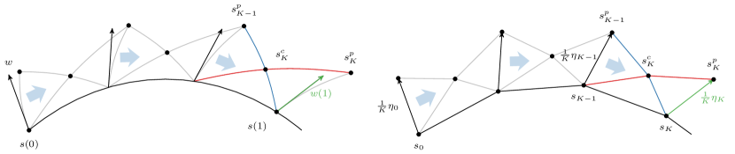
Figure 1: A sketch of the discretization of parallel transport via Schild’s ladder in the continuous context (left) and the discrete context (right).

More general discrete interpolation and extrapolation

In order to define subdivision curves we would like to compute discrete geodesic averaging not only at discrete time steps $\tfrac{k}{K}$ for $k=0,\dots,K$ but also for any arbitrary time $t\in[0,1]$ with $t$ not being a multiple of $\tfrac{1}{K}$. Therefore, we generalize the discrete interpolation operator in (10) as follows. We first compute a discrete geodesic of length $K+1$ as explained above. Then in a second step we use a weighted, discrete geodesic interpolation between the two shells $s_{\lfloor tK\rfloor}$ and $s_{\lfloor tK\rfloor+1}$ for which $t\in(\tfrac{\lfloor tK\rfloor}{K},\tfrac{\lfloor tK\rfloor+1}{K})$ and $\lfloor y\rfloor$ denotes the largest integer smaller than or equal to $y\in\mathbb{R}$ and $s_{k}=\mathbf{Av}^{K}\left(s_{A},s_{B},\tfrac{k}{K}\right)$. Thereby the weighted, discrete geodesic interpolation is given as

$$\mathbf{Av}^{K}(s_{A},s_{B},t)=\operatorname*{argmin}_{s\in\mathcal{S}}(1-t(K))\mathcal{W}[s_{\lfloor tK\rfloor},s]+t(K)\mathcal{W}[s,s_{\lfloor tK\rfloor+1}],$$ (11)

where $t(K)=tK-\lfloor tK\rfloor$ (cf. Fig. 2); e.g. for $t=\frac{2k+1}{2K}$ and $t(K)=\frac{1}{2}$ we retrieve the equal weighting from the definition of a $3$ shell discrete geodesic.

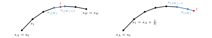
Figure 2: Sketch for the definition of the generalized interpolation operator (left) and the generalized exponential map (right).

In a similar manner we define a generalized exponential map for $t$ not being a multiple of the time step size $\tau=\tfrac{1}{K}$ for given $K$. To this end, we define ${\mathbf{Exp}}^{K}(t,\xi)$ such that $s_{k}:={\mathbf{Exp}}^{K}(k/K,\xi)$ for $k=\lfloor tK\rfloor$ is the weighted discrete geodesic average of $s_{k-1}={\mathbf{Exp}}^{K}((k-1)/K,\xi)$ and the unknown shell ${\mathbf{Exp}}^{K}(t,\xi)$ with weights $\tfrac{t(K)}{1+t(K)}$ and $\tfrac{1}{1+t(K)}$, i.e.

$$s_{k}=\operatorname*{argmin}_{\tilde{s}}\left(\frac{t(K)}{1+t(K)}\mathcal{W}[s_{k-1},\tilde{s}]+\frac{1}{1+t(K)}\mathcal{W}[\tilde{s},s]\right)$$

with unknown shell $s={\mathbf{Exp}}^{K}(t,\xi)$. This can be expressed in terms of the Euler-Lagrange equation

$$0=\frac{t(K)}{1+t(K)}\mathcal{W}_{,2}[s_{k-1},s_{k}]+\frac{1}{1+t(K)}\mathcal{W}_{,1}[s_{k},s]\,.$$

The solution is unique for sufficiently small $\xi$ (cf. Fig. 2). Obviously, for $t(K)=0$ we obtain ${\mathbf{Exp}}^{K}(t,\xi)=s_{k}$ and for $t(K)=1$ and thus $t=\tfrac{k+1}{K}$ the exponential map coincides with the previous definition of ${\mathbf{Exp}}^{K}(\tfrac{k+1}{K},\xi)$.

Implementation

For the discretization of shells in $\mathcal{S}$ we implemented a subdivision element method in C++ based on Loop’s subdivision functions. This scheme ensures $H^{2}$ regularity ($C^{2}$ apart from irregular vertices) of the limit function. Thus it allows for the energy densities used in the variational approximation of the path energy a conforming discretization in particular of the relative shape operator (cf. [11]). The crucial step in the implementation of subdivision methods is the choice of the numerical quadrature. Here, we use the mid-edge quadrature considered in [38] which displays a good compromise between efficiency and robustness. Additionally, this quadrature rule in conjunction with lookup tables allows for the simulation with input meshes containing more than one extraordinary vertex per patch. We refer to [38] for implementational details.

Figure 3: Control mesh and subdivision limit surface for the cactus (left) and the hand shape (right).

For the computations presented in the subsequent sections we used a cactus and a hand model (cf. Fig. 3 for an instance of the control meshes and the subdivision surfaces). The underlying meshes are closed and consist of 263 vertices for the cactus model and 305 vertices for the hand model.

The numerical computation of discrete geodesic, discrete logarithm, discrete exponential map and discrete parallel transport uses the elastic deformation energy defined in (4) with membrane and bending energy density given as in (5) and (6). In all computations the material parameters are chosen as follows: $\lambda=\mu=1.0$ and $\delta=0.01$. The nonlinear minimization of the discrete path energy (8) for the computation of discrete geodesics and geodesic extrapolation is performed by solving the corresponding set of Euler-Lagrange equations via Newton’s method with stepsize control. The iteration is stopped if the squared $\ell^{2}$-norm of the Newton step decreases below $\epsilon=10^{-4}$. Note that the performance of Newton’s method strongly depends on the initialization. While this does not pose a problem for the geodesic extrapolation where the unknown shell $s_{k}$ can be simply initialized with $s_{k-1}$ the issue is more delicate for geodesic interpolation. For the computation of discrete geodesics between to given shells $s_{0}$ and $s_{K}$ we therefore iteratively minimized the functionals

$$s\mapsto(K-k)\mathcal{W}[s_{0},s]+k\mathcal{W}[s,s_{K}]$$

for $k=1,\dots,K-1$ to get $s_{k}$, starting the $k$th interation with the inialization $s=s_{k-1}$. This approach yields a good initialization $(s_{0},\dots,s_{K})$ for the final Newton iteration such that in most cases Newton’s method is in the contraction region of quadratic convergence.

Using this numerical setup the computation times needed in the simulations for this paper range from a couple of minutes for the computation of simple quadratic Bézier curves to several hours for subdivision curves of levels higher than four.

3 Bézier curves in shell space

Now, we consider Bézier curves in the space of subdivision shell surfaces and derive a discrete counterpart of Riemannian Bézier curves using the discretization from [34] and following [6] adapted to the space of subdivision shell surfaces. Consider a set of control shells $(s_{0}^{0},\ldots,s_{n}^{0})$ with $s_{j}^{0}\in\mathcal{S}$ for $j=0,\ldots,n$ and the mapping

$${\mathcal{B}}:\underbrace{\mathcal{S}\times\ldots\times\mathcal{S}}_{n+1}\times[0,1]\to\mathcal{S}$$

which is recursively defined via the de Casteljau algorithm

$${\mathcal{B}}(s_{i},\ldots,s_{j},t)=\mathcal{Av}({\mathcal{B}}(s_{i},\ldots,s_{j-1},t),{\mathcal{B}}(s_{i+1},\ldots,s_{j},t),t)$$

for $i,j\in\{0,\ldots,n\}$ with $i<j$ and ${\mathcal{B}}(s,t)=s$. In other words for $(s_{0}^{0},\ldots,s_{n}^{0})$ and fixed $t\in[0,1]$ we compute for $j=1,\ldots,n$ and $i=j,\ldots,n$ the shells

$$s_{i}^{j} =\mathcal{Av}(s_{i-1}^{j-1},s_{i}^{j-1},t)$$

and after $n$ steps we obtain the shell ${\mathcal{B}}(s_{0}^{0},\ldots,s_{n}^{0},t)=s_{n}^{n}$. The resulting curve $({\mathcal{B}}(s_{0}^{0},\ldots,s_{n}^{0},t))_{t\in[0,1]}$ is denoted a Bézier curve in shell space of degree $n$. Compared to the Euclidean case the shells $s_{i}^{j}$ do not lie on a straight line but on a geodesic $(\mathcal{Av}(s_{i-1}^{j-1},s_{i}^{j-1},t))_{t\in[0,1]}$ connecting $s_{i-1}^{j-1}$ with $s_{i}^{j-1}$.

Now, we transfer the concept of Riemannian Bézier curves to our time-discrete setup. Again, we consider a set of control shells $(s_{0}^{0},\ldots,s_{n}^{0})$ with $s_{j}^{0}\in\mathcal{S}$ for $j=0,\ldots,n$ and some $K\in\mathbb{N}$. Then we define a mapping

$${\mathbf{B}^{K}}:\underbrace{\mathcal{S}\times\ldots\times\mathcal{S}}_{n+1}\times\{0,\tfrac{1}{K},\ldots,\tfrac{K}{K}\}\to\mathcal{S}$$

recursively via the following discrete de Casteljau algorithm

$${\mathbf{B}^{K}}(s_{i},\ldots,s_{j},\tfrac{k}{K})=\mathbf{Av}^{K}({\mathbf{B}^{K}}(s_{i},\ldots,s_{j-1},\tfrac{k}{K}),{\mathbf{B}^{K}}(s_{i+1},\ldots,s_{j},\tfrac{k}{K}),\tfrac{k}{K})$$

for $i,j\in\{0,\ldots,n\}$ with $i<j$, $k\in\{0,\ldots,K\}$, and ${\mathbf{B}^{K}}(s,\tfrac{k}{K})=s$ . For the evaluation of a Bézier curve of degree $n$ with input shells $(s_{0}^{0},\ldots,s_{n}^{0})$, and for $K\in\mathbb{N}$ the discrete de Casteljau algorithm for $k\in\{0,\ldots,K\}$ reads as follows

  for $j=1$ to $n$ do

     for $i=j$ to $n$ do

        $s^{j}_{i}=\mathbf{Av}^{K}(s^{j-1}_{i-1},s^{j-1}_{i},\tfrac{k}{K})$

     end for

  end for

  ${\mathbf{B}^{K}}(s_{0}^{0},\ldots,s_{n}^{0},\tfrac{k}{K})=s_{n}^{n}$.

In analogy to the continuous Bézier curve we call the resulting discrete path

$$({\mathbf{B}^{K}}(s_{0},\ldots,s_{n},\tfrac{k}{K}))_{k\in\{0,\ldots,K\}}$$

a discrete Bézier curve in shell space of degree $n$ (see Figures 4,5, and 6). Let us remark that the evaluation of the Bézier curve for general times $t\in[0,1]$, which are not multiples of $\tfrac{1}{K}$ is straightforward using the the generalized interpolation.

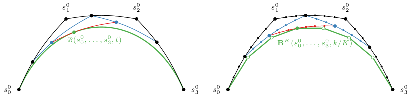
Figure 4: Sketch of the continuous (left) and discrete (right) Riemannian de Casteljau algorithm defining a continuous and a discrete cubic Bézier curve, respectively (the algorithm proceeds as follows: ).

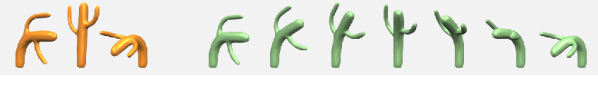
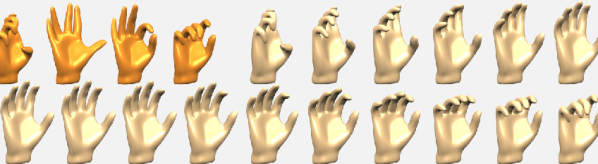
Figure 5: Two discrete Bézier curves for the cactus ($K=6$, green) and the hand model ($K=15$, beige). The control shells are shown in orange on the left.

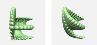
Figure 6: Comparison between a piecewise geodesic paths (left) and a quadratic Bézier curve (right).

4 Time-discrete cardinal splines in shell space

In what follows we will use the relation between cubic Bézier curves and cubic Hermite curves [25] to define discrete cardinal splines in this space. To this end, we first recall that a cubic Hermite curve $t\mapsto{\mathcal{H}}(s_{A},v_{A},v_{B},s_{B},t)$ with endpoints $s_{A}$ and $s_{B}$ and with initial and final velocity $v_{A}\in T_{s_{A}}\mathcal{S}$ and $v_{B}\in T_{s_{B}}\mathcal{S}$, respectively, coincides with the Bézier curve $t\mapsto{\mathcal{B}}(s_{0},s_{1},s_{2},s_{3},t)$, where

$$s_{0} =s_{A}\,,\quad s_{1}=\exp_{s_{A}}(\tfrac{1}{3}v_{A})\,,\quad s_{2}=\exp_{s_{B}}(-\tfrac{1}{3}v_{B})\,,\quad s_{3}=s_{B}\,.$$

From this we immediately derive the discrete counterpart and define the discrete cubic Hermite curve

$$({\mathbf{H}^{K}}(s_{A},\xi_{A},\xi_{B},s_{B},\tfrac{k}{K}))_{k\in\{0,\ldots,K\}}$$

for given shells $s_{A},s_{B}\in\mathcal{S}$, displacements $\xi_{A}$, $\xi_{B}$ as approximations of the tangent vectors $v_{A}$ and $v_{B}$, respectively, and $K>1$ by

$${\mathbf{H}^{K}}(s_{A},\xi_{A},\xi_{B},s_{B},\tfrac{k}{K})={\mathbf{B}^{K}}(s_{0},s_{1},s_{2},s_{3},\tfrac{k}{K})\quad\text{where}$$

$$s_{0}=s_{A}\,,\quad s_{1}={\mathbf{Exp}}^{K}_{s_{A}}(\frac{1}{3},\xi_{A})\,,\quad s_{2}={\mathbf{Exp}}^{K}_{s_{B}}(\frac{1}{3},-\xi_{B})\,,\quad s_{3}=s_{B}.$$

Let us remark that for $k$ being a multiple of $3$ the term ${\mathbf{Exp}}^{K}_{s_{A}}(\frac{1}{3},\xi_{A})$ requires $\tfrac{K}{3}$ steps of the iterative scheme for the discrete exponential map. Now, we are in the position to discuss continuous cardinal splines on the Riemannian manifold $\mathcal{S}$ of shells and to derive a proper discrete cardinal spline. Cardinal splines interpolate the given sequence of control shells. In between each consecutive pair of control points the cardinal spline coincides with a cubic Hermite curve with the same pair of end shells. The velocities at the end shells of such a Hermite curve are computed via parallel transport of the initial velocity of the geodesic pointing from the previous to the next shell. An exception is only the velocity at the first and the last shell. The latter mechanism ensures differentiability of the resulting spline curve. In detail, for a sequence of shells $(s_{0},\ldots,s_{m})$ with $s_{j}\in\mathcal{S}$ for $j=0,\ldots,m$, $m\geq 2$ and $\kappa\in[0,3]$ consider the mapping

$${\mathcal{CS}}_{\kappa}:\underbrace{\mathcal{S}\times\ldots\times\mathcal{S}}_{m+1}\times[0,m]\to\mathcal{S}$$

which is defined piecewise for $t\in[l,l+1]$ where $l=0,\ldots,m-1$ by

$${\mathcal{CS}}_{\kappa}(s_{0},\ldots,s_{m},t)={\mathcal{B}}(d_{3l},d_{3l+1},d_{3l+2},d_{3l+3},t-l)\,.$$

To ensure the interpolation condition we have to set

$$d_{3j} =s_{j},\qquad j=0,\ldots,m\,.$$

On the left and on the right we prescribe boundary conditions via

$$d_{1} =\mathcal{Av}(s_{0},s_{1},{}^{\kappa}\!/_{3}),$$

$$d_{3m-1} =\mathcal{Av}(s_{m-1},s_{m},1-{}^{\kappa}\!/_{3})=\mathcal{Av}(s_{m},s_{m-1},{}^{\kappa}\!/_{3})\,.$$

In explicit, this ensures that $\frac{\mathrm{d}}{\mathrm{d}t}{\mathcal{CS}}_{\kappa}(s_{0},\ldots,s_{m},t)$ is parallel to $\log_{d_{0}}(d_{1})$ for $t=0$ and to $\log_{d_{3m}}(d_{3m-1})$ for $t=m$ . Finally, we prescribe for each $j\in 1,\ldots,m-1$ the control points $d_{3j-1}$ and $d_{3j+1}$ . To this end, we first compute the initial velocity $w_{j}$ of the geodesic from $d_{3(j-1)}$ and $d_{3(j+1)}$ and scale it with ${}^{\kappa}\!/_{3}$, where $\kappa$ is the tension factor, which controls the inflection behaviour of the cardinal spline:

$$w_{j} =\tfrac{\kappa}{3}\log_{s_{j-1}}(s_{j+1})\,.$$

Then we transport this velocity along the geodesic from $s_{j-1}$ to $s_{j}$ and use the exponential map in the positive and negative direction of the transported velocity field to define the remaining control points:

$$w_{j}^{p} ={\mathrm{P}}_{(\mathcal{Av}(s_{j-1},s_{j},t))_{t\in[0,1]}}(w_{j}),$$

$$d_{3j-1} =\exp_{s_{j}}(-w_{j}^{p}),$$

$$d_{3j+1} =\exp_{s_{j}}(w_{j}^{p})\,.$$

For the computation of the shells $d_{3j-1}$ and $d_{3j+1}$ we refer to the sketch in Figure 7. The resulting curve

$$({\mathcal{CS}}_{\kappa}(s_{0},\ldots,s_{m},t))_{t\in[0,m]}$$

defines the cubic cardinal spline in shell space with tension parameter $\kappa\in[0,3]$ .

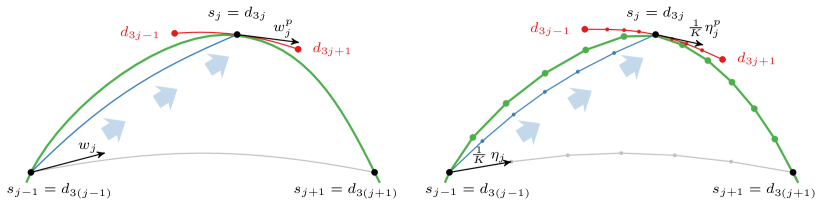
Figure 7: Sketch of the construction of the control shells $d_{3j-1}$ and $d_{3j+1}$ for the cardinal spline in the continuous (left) and discrete (right) setting (the algorithm proceeds as follows: ).

This construction can be transferred to the discrete context to define the corresponding discrete cardinal spline. Again we take into account a sequence of control shells $(s_{0},\ldots,s_{m})$ with $s_{j}\in\mathcal{S}$ for $j=0,\ldots,m$, $m\geq 2$ and $K\geq 2$ and define the mapping

$${\mathbf{CS}^{K}_{\kappa}}:\underbrace{\mathcal{S}\times\ldots\times\mathcal{S}}_{m+1}\times\{0,\tfrac{1}{K},\ldots,m\cdot\tfrac{K}{K}\}\to\mathcal{S}$$

which is given piecewise for $k\in[l\cdot K,\ldots,(l+1)\cdot K]$ as $l=0,\ldots,m-1$ by

$${\mathbf{CS}^{K}_{\kappa}}(s_{0},\ldots,s_{m},\tfrac{k}{K})={\mathbf{B}^{K}}(d_{3l},d_{3l+1},d_{3l+2},d_{3l+3},\tfrac{k}{K}-l)\,,$$

where the interpolation control points are copied as before, i.e.

$$d_{3j} =s_{j},\qquad j=0,\ldots,m\,.$$

The discrete counterparts of the boundary conditions are

$$d_{1} ={\mathbf{Exp}}^{K}_{s_{0}}\left({}^{\kappa}\!/_{3},{\mathbf{Log}}^{K}_{s_{0}}(s_{1})\right),$$

$$d_{3m-1} ={\mathbf{Exp}}^{K}_{s_{m}}\left({}^{\kappa}\!/_{3},{\mathbf{Log}}^{K}_{s_{m}}(s_{m-1})\right)\,.$$

The control points $d_{3j-1}$ and $d_{3j+1}$ for $j\in 1,\ldots,m-1$ are determined as follows:

$$\eta_{j} ={\mathbf{Log}}^{K}_{s_{j-1}}(s_{j+1})\,,$$

$$\eta_{j}^{p} ={\mathbf{P}}^{K}_{(\mathbf{Av}^{K}(s_{j-1},s_{j},\tfrac{k}{K}))_{k=\{0,\ldots,K\}}}\left(\eta_{j}\right)\,,$$

$$d_{3j-1} ={\mathbf{Exp}}^{K}_{s_{j}}\left(\tfrac{\kappa}{3},-\eta_{j}^{p}\right)\,,$$

$$d_{3j+1} ={\mathbf{Exp}}^{K}_{s_{j}}\left(\tfrac{\kappa}{3},\eta_{j}^{p}\right)\,.$$

(see also Figure 7). We call the resulting curve $({\mathbf{CS}^{K}_{\kappa}}(s_{0},\ldots,s_{m},\tfrac{k}{K}))_{k\in\{0,\ldots,m\cdot K\}}$ the discrete cubic cardinal spline in shell space with tension $\kappa\in[0,3]$. Let us emphasize that this is equivalent to the construction with discrete cubic Hermite splines where a segment consists of the shells $s_{j}$ and $s_{j+1}$ and displacements $\eta_{j-1}^{p}$ and $-\eta_{j}^{p}$. Examples are given in Figure 8.

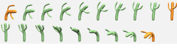
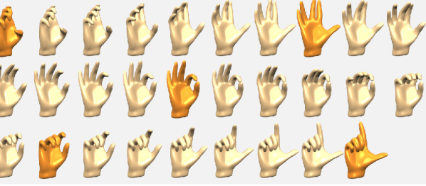
Figure 8: Two discrete cardinal spline curves for the cactus (green, $K=9$) and the hand model (beige, $K=7$). The interpolated key frames are shown in orange.

5 Interpolatory subdivision curves in shell space

In this section we transfer the concept of unitary subdivision to shell space in order to compute smooth interpolation curves for a given set of key frame shells. In Euclidean space a subdivision curve is defined as the limit of increasingly fine control polygons subject to a small set of subdivision rules. Replacing straight lines by geodesic paths, this construction can be transferred to the Riemannian setting. For this purpose we make use of the extension of the geodesic averaging operator and the exponential map in Section 2. Furthermore, for the ease of presentation we generalize the averaging $\mathcal{Av}$ to an interpolation $\mathcal{I}$, which is also defined for $t\not\in[0,1]$. In explicit, $\mathcal{I}$ is given as follows:

$$\mathcal{I}(s_{A},s_{B},t) =\mathcal{Av}(s_{A},s_{B},t) \qquad\quad\mbox{ for }0\leq t\leq 1\,,$$

$$\mathcal{I}(s_{A},s_{B},t) =\exp_{s_{A}}(t\log_{s_{A}}(s_{B})) \qquad\quad\mbox{ for }t<0\,,$$

$$\mathcal{I}(s_{A},s_{B},t) =\exp_{s_{B}}(-(t-1)\log_{s_{B}}(s_{A})) \qquad\quad\mbox{ for }t>1\,.$$

The same notational generalization can be performed for the discrete averaging:

$$\mathbf{I}^{K}(s_{A},s_{B},t) =\mathbf{Av}^{K}(s_{A},s_{B},t) \quad\mbox{ for }0\leq t\leq 1\,,$$

$$\mathbf{I}^{K}(s_{A},s_{B},t) ={\mathbf{Exp}}^{K}_{s_{A}}(-t,-{\mathbf{Log}}^{K}_{s_{A}}(s_{B})) \quad\mbox{ for }t<0\,,$$

$$\mathbf{I}^{K}(s_{A},s_{B},t) ={\mathbf{Exp}}^{K}_{s_{B}}((t-1),-{\mathbf{Log}}^{K}_{s_{B}}(s_{A})) \quad\mbox{ for }t>1\,.$$

In the following we state the subdivision rules for the interpolatory binary four- and six-point schemes as well as the interpolatory ternary four-point scheme. Let us emphasize that these rules depends on a proper combination of (discrete) geodesic interpolation and extrapolation via the (discrete) exponential map, both encoded in the generalized interpolation operators $\mathcal{I}$ and $\mathbf{I}^{K}$.

To this end, let us consider a set of initial shells $s_{0}^{0},\dots,s_{n}^{0}\in\mathcal{S}$ with $n\geq 2$. The Riemannian interpolatory binary four-point scheme defines the corresponding control shells $s_{k}^{\ell}$ of level $\ell>0$ iteratively by

$$s_{2k}^{\ell} =s_{k}^{\ell-1},\quad s_{2k+1}^{\ell}=\mathcal{I}(d_{2k}^{\ell-1},d_{2k+1}^{\ell-1},\tfrac{1}{2}),$$

for $k=0,\dots,2^{\ell}n$ with

$$d_{2k}^{\ell-1} =\mathcal{I}(s_{k-1}^{\ell-1},s_{k}^{\ell-1},\tfrac{9}{8}),\quad d_{2k+1}^{\ell-1}=\mathcal{I}(s_{k+2}^{\ell-1},s_{k+1}^{\ell-1},\tfrac{9}{8})$$

(cf. the sketch in Fig. 9). Similarly the Riemannian interpolatory binary six-point scheme is given by

$$s_{2k}^{\ell} =s_{k}^{\ell-1},\quad s_{2k+1}^{\ell}=\mathcal{I}(d_{4k+2}^{\ell-1},d_{4k+3}^{\ell-1},\tfrac{1}{2}),$$

for $k=0,\dots,2^{\ell}n$, where

$$d_{4k}^{\ell-1} =\mathcal{I}(s_{k-2}^{\ell-1},s_{k-1}^{\ell-1},\tfrac{25}{22}),\quad d_{4k+1}^{\ell-1} =\mathcal{I}(s_{k+3}^{\ell-1},s_{k+2}^{\ell-1},\tfrac{25}{22}),$$

$$d_{4k+2}^{\ell-1} =\mathcal{I}(d_{4k}^{\ell-1},s_{k}^{\ell-1},\tfrac{75}{64}),\quad d_{4k+3}^{\ell-1} =\mathcal{I}(d_{4k+1}^{\ell-1}s_{k+1}^{\ell-1},\tfrac{75}{64}).$$

Finally the interpolatory ternary four-point scheme consists of the rules

$$s_{3k}^{\ell} =s_{k}^{\ell-1},\quad s_{3k+1}^{\ell}=\mathcal{I}(d_{4k}^{\ell-1},d_{4k+1}^{\ell-1},\tfrac{10}{33}),\quad s_{3k+2}^{\ell}=\mathcal{I}(d_{4k+2}^{\ell-1},d_{4k+3}^{\ell-1},\tfrac{10}{33}),$$

with $k=0,\dots,3^{\ell}n$, and

$$d_{4k}^{\ell-1} =\mathcal{I}(s_{k-1}^{\ell-1},s_{k}^{\ell-1},\tfrac{76}{69}),\quad d_{4k+1}^{\ell-1} =\mathcal{I}(s_{k+1}^{\ell-1},s_{k+2}^{\ell-1},-\tfrac{2}{15}),$$

$$d_{4k+2}^{\ell-1} =\mathcal{I}(s_{k+2}^{\ell-1},s_{k+1}^{\ell-1},\tfrac{76}{69}),\quad d_{4k+3}^{\ell-1} =\mathcal{I}(s_{k}^{\ell-1},s_{k-1}^{\ell-1},-\tfrac{2}{15}).$$

In order to transfer these subdivision rules into the time-discrete setup we replace the time-continuous (generalized) interpolation operator by its time-discrete counterpart. For $K\geq 2$ and for the set of keyframe shells $s_{0}^{0},\dots,s_{n}^{0}\in\mathcal{S}$ (our control shells) with $n\geq 2$ we obtain the interpolatory, discrete Riemannian binary four-point scheme with shells $s_{k}^{\ell}$ on level $\ell>0$ iteratively defined by

$$s_{2k}^{\ell} =s_{k}^{\ell-1},\quad s_{2k+1}^{\ell}=\mathbf{I}^{K}(d_{2k}^{\ell-1},d_{2k+1}^{\ell-1},\tfrac{1}{2}),$$

for $k=0,\dots,2^{\ell}n$ with

$$d_{2k}^{\ell-1} =\mathbf{I}^{K}(s_{k-1}^{\ell-1},s_{k}^{\ell-1},\tfrac{9}{8}),\quad d_{2k+1}^{\ell-1}=\mathbf{I}^{K}(s_{k+2}^{\ell-1},s_{k+1}^{\ell-1},\tfrac{9}{8})$$

(cf. the sketch in Fig. 9). The discrete binary six-point scheme reads as follows

$$s_{2k}^{\ell} =s_{k}^{\ell-1},\quad s_{2k+1}^{\ell}=\mathbf{I}^{K}(d_{4k+2}^{\ell-1},d_{4k+3}^{\ell-1},\tfrac{1}{2}),$$

for $k=0,\dots,2^{\ell}n$, where

$$d_{4k}^{\ell-1} =\mathbf{I}^{K}(s_{k-2}^{\ell-1},s_{k-1}^{\ell-1},\tfrac{25}{22}),\quad d_{4k+1}^{\ell-1} =\mathbf{I}^{K}(s_{k+3}^{\ell-1},s_{k+2}^{\ell-1},\tfrac{25}{22}),$$

$$d_{4k+2}^{\ell-1} =\mathbf{I}^{K}(d_{4k}^{\ell-1},s_{k}^{\ell-1},\tfrac{75}{64}),\quad d_{4k+3}^{\ell-1} =\mathbf{I}^{K}(d_{4k+1}^{\ell-1}s_{k+1}^{\ell-1},\tfrac{75}{64}).$$

For the discrete ternary four-point scheme we get

$$s_{3k}^{\ell} =s_{k}^{\ell-1},\quad s_{3k+1}^{\ell}=\mathbf{I}^{K}(d_{4k}^{\ell-1},d_{4k+1}^{\ell-1},\tfrac{10}{33}),\quad s_{3k+2}^{\ell}=\mathbf{I}^{K}(d_{4k+2}^{\ell-1},d_{4k+3}^{\ell-1},\tfrac{10}{33}),$$

with $k=0,\dots,3^{\ell}n$, and

$$d_{4k}^{\ell-1} =\mathbf{I}^{K}(s_{k-1}^{\ell-1},s_{k}^{\ell-1},\tfrac{76}{69}),\quad d_{4k+1}^{\ell-1} =\mathbf{I}^{K}(s_{k+1}^{\ell-1},s_{k+2}^{\ell-1},-\tfrac{2}{15}),$$

$$d_{4k+2}^{\ell-1} =\mathbf{I}^{K}(s_{k+2}^{\ell-1},s_{k+1}^{\ell-1},\tfrac{76}{69}),\quad d_{4k+3}^{\ell-1} =\mathbf{I}^{K}(s_{k}^{\ell-1},s_{k-1}^{\ell-1},-\tfrac{2}{15}).$$

Examples for the different subdivision schemes in shell space are given in Figures 10 and 12 and a comparison is shown in Figure 11.

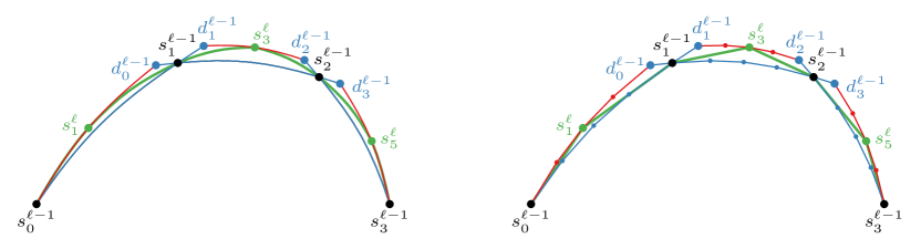
Figure 9: Sketch of the construction for the interpolatory binary four-point scheme in the continuous case (left) and the discrete case (right) (the algorithm proceeds as follows: ).

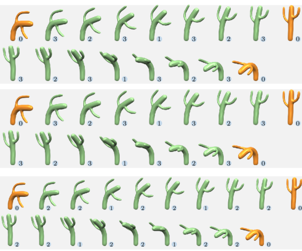
Figure 10: Different discrete subdivision curves interpolate three different poses of the cactus shell (orange): discrete binary four-point scheme (top), discrete binary six-point scheme (middle), discrete ternary four-point scheme. The numbers indicate the level of refinement.

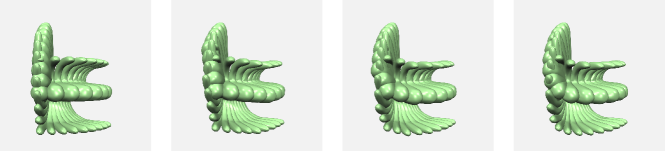
Figure 11: Comparison for binary 4-point rule for level $l=0,\,1,\,2,\,3$ .

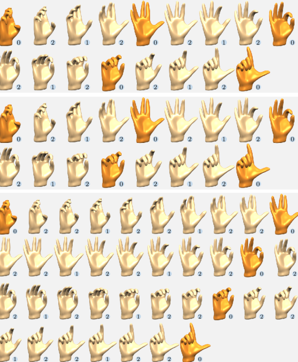
Figure 12: As above in Fig. 10 different discrete subdivision curves now interpolate five different poses of the hand model (orange): discrete binary four-point scheme (top), discrete binary six-point scheme (middle), discrete ternary four-point scheme. Again the numbers indicate the level of refinement.

6 Discussion

We have generalized the notion of different interpolating curves, namely cardinal splines, and three different types of interpolatory subdivision schemes for curves to the Riemannian manifold of shells. This methodology turns into a computationally efficient toolbox via the implementation of a variational time discretization of geodesic interpolation, extrapolation via a discrete geometric exponential map, discrete geometric logarithm, and discrete parallel transport. Due to the physical foundation of the underlying Riemannian metric on the space of shells the application to subdivision shell surfaces led to physically intuitive interpolation curves in shell space.

The use of subdivision surfaces to represent shells allows a conforming discretization of the path energy and does not require any discrete geometry version of the relative shape operator. In particular, approximating a given smooth surface with subdivision surfaces generated by an increasing number of control points we can expect convergence of the relative shape operator. Concerning the numerical implementation Newton’s method is used in particular to solve the geodesic interpolation problem, which requires the minimization of a nonlinear energy over $K-1$ coupled control meshes of the subdivision shells. Here the hierarchical approach incorporated in the subdivision method is particularly well-suited. It ensures that Newton’s method is in most cases (especially on finer levels of the subdivision scheme) in the contraction region of quadratic convergence.

We remark that the construction of the interpolating curves presented in this paper is entirely based on the solution of problems that are local in time. However, the corresponding functionals subject to minimization are non-convex such that the Newton solver may terminate in local minima which could possibly lead to discontinuities and non-uniqueness of the resulting interpolation curves. In the application this problem can be prevented by a good initialization of the Newton iteration (like the iterative initialization presented in Section 2) and a suitable choice of the step size $\tau=1/K$. We never encountered the described problem in any of our computations.

Compared to the Riemannian spline approach by Heeren et al. [33] we have to solve solely local problems in time, whereas in [33] a fully coupled global optimization problem with a large set of nonlinear constraints has to be solved. Furthermore, we do not require the simplification via the $L\Theta A$ approach for more complex shell models, which requires a back projection onto the manifold of shell surfaces. On the other hand our approach follows the paradigms of constructive approximation and lacks an energy minimizing interpretation.

Furthermore, the convergence behaviour of the sequence of subdivision curves to a smooth limit surfaces is open in particular for fixed time step size $\tau=\tfrac{1}{K}$. The proximity condition approach by Wallner and Dyn  [62] might be a good starting points to study smoothness properties. In our case two types of perturbations have to be considered: the perturbation due to the curviness of the manifold and the perturbation caused by our variational approximation of geodesics. Recently, Wallner [61] proved convergence of the linear four-point scheme and other univariate interpolatory schemes in Riemannian manifolds. To this end he studied Riemannian edge length contractivity of the schemes on a manifold combined with a multiresolutional analysis. Indeed, to apply these results certain consistency results of the path length of geodesic edges and the corresponding discrete path length are already known (cf. [53]).

References

- [1] Absil, P.-A., Gousenbourger, P.-Y., Striewski, P., and Wirth, B. Differentiable piecewise-Bézier surfaces on Riemannian manifolds. SIAM Journal on Imaging Sciences (2016). accepted.
- [2] Adams, B., Ovsjanikov, M., Wand, M., Seidel, H.-P., and Guibas, L. J. Meshless modeling of deformable shapes and their motion. Proceedings of the 2008 ACM SIGGRAPH/Eurographics Symposium on Computer Animation (2008).
- [3] Arden, G. Approximation Properties of Subdivision Surfaces. PhD thesis, University of Washington, 2001.
- [4] Bauer, M., and Bruveris, M. A new Riemannian setting for surface registration. In Proc. of MICCAI Workshop on Mathematical Foundations of Computational Anatomy (2011), pp. 182–194. arXiv:1106.0620.
- [5] Bauer, M., Harms, P., and Michor, P. W. Sobolev metrics on shape space of surfaces. J. Geom. Mech. 3, 4 (2011), 389–438.
- [6] Brandt, C., von Tycowicz, C., and Hildebrandt, K. Geometric flows of curves in shape space for processing motion of deformable objects. Comput. Graph. Forum 35, 2 (2016), 295–305.
- [7] Bronstein, A. M., Bronstein, M. M., and Kimmel, R. Topology-invariant similarity of nonrigid shapes. Inter. J. Comput. Vision 81, 3 (2009), 281–301.
- [8] Camarinha, M., Silva Leite, F., and Crouch, P. On the geometry of Riemannian cubic polynomials. Diff. Geom. Appl. 15 (2001), 107–135.
- [9] Cashman, T. J. Beyond Catmull-Clark? A survey of advances in subdivision surface methods. Computer Graphics Forum 31, 1 (2012), 42–61.
- [10] Catmull, E., and Clark, J. Recursively generated B-spline surfaces on arbitrary topological meshes. Computer Aided Design 10 (1978), 350–355.
- [11] Ciarlet, P. G. Mathematical elasticity. Vol. III, vol. 29 of Studies in Mathematics and its Applications. North-Holland Publishing Co., Amsterdam, 2000. Theory of shells.
- [12] Cirak, F., and Long, Q. Subdivision shells with exact boundary control and non–manifold geometry. Internat. J. Numer. Methods Engrg. 88, 9 (2011), 897–923.
- [13] Cirak, F., and Ortiz, M. Fully C1–conforming subdivision elements for finite deformation thin–shell analysis. Internat. J. Numer. Methods Engrg. 51(7) (2001), 813–833.
- [14] Cirak, F., Ortiz, M., and Schröder, P. Subdivision surfaces: a new paradigm for thin-shell finite–element analysis. Internat. J. Numer. Methods Engrg. 47, 12 (2000), 2039–72.
- [15] Cirak, F., Scott, M. J., Antonsson, E. K., Ortiz, M., and Schröder, P. Integrated modeling, finite–element analysis and engineering design for thin–shell structures using subdivision. Comput.-Aided Des. 34, 2 (2002), 137–148.
- [16] Crouch, P., and Silva Leite, F. The dynamic interpolation problem: On Riemannian manifold, Lie groups and symmetric spaces. J. Dynam. Control Systems 1, 2 (1995), 177–202.
- [17] DeRose, T., Kass, M., and Truong, T. Subdivision Surfaces in Character Animation. In Proceedings of the 25th Annual Conference on Computer Graphics and Interactive Techniques (1998), SIGGRAPH ’98, pp. 85–94.
- [18] do Carmo, M. P. Riemannian geometry. Birkhäuser Boston Inc., 1992. Translated from the second Portuguese edition.
- [19] Doo, D., and Sabin, M. Behaviour of recursive division surfaces near extraordinary points. Computer-Aided Design 10(6) (1978), 356–360.
- [20] Duchamp, T., Xie, G., and Yu, T. Single basepoint subdivision schemes for manifold-valued data: time-symmetry without space-symmetry. Found. Comput. Math. 13, 5 (2013), 693–728.
- [21] Dyn, N. Interpolatory subdivision schemes. In Tutorials on Multiresolution in Geometric Modelling, A. Iske, E. Quak, and M. S. Floater, Eds. Springer, Berlin, 2002, pp. 25–50.
- [22] Dyn, N., Grohs, P., and Wallner, J. Approximation order of interpolatory nonlinear subdivision schemes. J. Comput. Appl. Math. 233, 7 (2010), 1697–1703.
- [23] Effland, A., Rumpf, M., Simon, S., Stahn, K., and Wirth, B. Bézier curves in the space of images. In Proc. of International Conference on Scale Space and Variational Methods in Computer Vision, vol. 9087 of Lecture Notes in Computer Science. Springer, Cham, 2015, pp. 372–384.
- [24] Ehlers, J., Pirani, F. A. E., and Schild, A. The geometry of free fall and light propagation. In General relativity (papers in honour of J. L. Synge). Clarendon Press, Oxford, 1972, pp. 63–84.
- [25] Farin, G. Curves and Surfaces for CAGD: A Practical Guide, 5th ed. Morgan Kaufmann Publishers Inc., San Francisco, CA, USA, 2002.
- [26] Fröhlich, S., and Botsch, M. Example-driven deformations based on discrete shells. Comput. Graph. Forum 30, 8 (2011), 2246–2257.
- [27] Giambo, R., and Giannoni, F. An analytical theory for Riemmanian cubic polynomials. IMA Journal of Mathematical Control and Information 19 (2002), 445–460.
- [28] Gousenbourger, P.-Y., Samir, C., and Absil, P. Piecewise-bezier c1 interpolation on riemannian manifolds with application to 2d shape morphing. In Pattern Recognition (ICPR), 2014 22nd International Conference on (2014), pp. 4086–4091.
- [29] Green, S., and Turkiyyah, G. Second Order Accurate Constraint Formulation for Subdivision Finite Element Simulation of Thin Shells. International Journal For Numerical Methods In Engineering 61, 3 (2004), 380–405.
- [30] Green, S., Turkiyyah, G., and Storti, D. Subdivision–Based Multilevel Methods for Large Scale Engineering Simulation of Thin Shells. In Proceedings of ACM Solid Modeling (2002).
- [31] Grohs, P. A general proximity analysis of nonlinear subdivision schemes. SIAM J. Math. Anal. 42, 2 (2010), 729–750.
- [32] Heeren, B., Rumpf, M., Schröder, P., Wardetzky, M., and Wirth, B. Exploring the geometry of the space of shells. Comput. Graph. Forum 33, 5 (2014), 247–256.
- [33] Heeren, B., Rumpf, M., Schröder, P., Wardetzky, M., and Wirth, B. Splines in the space of shells. Comput. Graph. Forum 35, 5 (2016), 111–120.
- [34] Heeren, B., Rumpf, M., Wardetzky, M., and Wirth, B. Time-discrete geodesics in the space of shells. Comput. Graph. Forum 31, 5 (2012), 1755–1764.
- [35] Hinkle, J., Muralidharan, P., Fletcher, P. T., and Joshi, S. Polynomial regression on Riemannian manifolds. In Proc. of European Conference on Computer Vision (2012), vol. 7574 of Lecture Notes in Computer Science, pp. 1–14.
- [36] Hofer, M., and Pottmann, H. Energy-minimizing splines in manifolds. ACM Trans. Graph. 23, 3 (2004), 284–293.
- [37] Jin, M., Zeng, W., Luo, F., and Gu, X. Computing teichmüller shape space. IEEE Transactions on Visualization and Computer Graphics 15, 3 (2009), 504–517.
- [38] Jüttler, B., Mantzaflaris, A., Perl, R., and Rumpf, M. On numerical integration in isogeometric subdivision methods for PDEs on surfaces. Computer Methods in Applied Mechanics and Engineering 302 (2016), 131–146.
- [39] Kass, M., and Anderson, J. Animating oscillatory motion with overlap: Wiggly splines. ACM Trans. Graph. 27, 3 (2008), 28:1–28:8.
- [40] Kheyfets, A., Miller, W. A., and Newton, G. A. Schild’s ladder parallel transport procedure for an arbitrary connection. Internat. J. Theoret. Phys. 39, 12 (2000), 2891–2898.
- [41] Kilian, M., Mitra, N. J., and Pottmann, H. Geometric modeling in shape space. ACM Trans. Graph. 26 (2007), 1–8.
- [42] Kurtek, S., Klassen, E., Ding, Z., and Srivastava, A. A novel Riemannian framework for shape analysis of 3D objects. In Proc. of IEEE Conference on Computer Vision and Pattern Recognition (2010), pp. 1625–1632.
- [43] Kurtek, S., Klassen, E., Gore, J. C., Ding, Z., and Srivastava, A. Elastic geodesic paths in shape space of parametrized surfaces. IEEE Trans. Pattern Anal. Mach. Intell. 34, 9 (2012), 1717–1730.
- [44] Liu, X., Shi, Y., Dinov, I., and Mio, W. A computational model of multidimensional shape. Int. J. Comput. Vis. 89, 1 (2010), 69–83.
- [45] Loop, C. Smooth spline surfaces over irregular meshes. In SIGGRAPH ’94: Proceedings of the 21st annual conference on Computer graphics and interactive techniques (1994), ACM Press, pp. 303–310.
- [46] Noakes, L., Heinzinger, G., and Paden, B. Cubic splines on curved spaces. IMA J. Math. Control Inform. 6, 4 (1989), 465–473.
- [47] Peters, J., and Reif, U. Subdivision Surfaces. Springer Series in Geometry and Computing, 2008.
- [48] Peters, J., and Wu, X. On the local linear independence of generalized subdivision functions. SIAM Journal on Numerical Analysis (SINUM) 44, 6 (2006), 2389–2407.
- [49] Popiel, T., and Noakes, L. Bézier curves and interpolation in Riemannian manifolds. J. Approx. Theory 148, 2 (2007), 111–127.
- [50] Pottmann, H., and Hofer, M. A variational approach to spline curves on surface. Comput. Aided Geom. Design 22, 7 (2005), 693–709.
- [51] Reif, U. A unified approach to subdivision algorithms near extraordinary vertices. Comput. Aided Geom. Design 12, 2 (1995), 153–174.
- [52] Reif, U., and Schröder, P. Curvature integrability of subdivision surfaces. Adv. Comput. Math. 14, 2 (2001), 157–174.
- [53] Rumpf, M., and Wirth, B. Variational time discretization of geodesic calculus. IMA J. Numer. Anal. 35, 3 (2015), 1011–1046.
- [54] Schulz, C., von Tycowicz, C., Seidel, H.-P., and Hildebrandt, K. Animating deformable objects using sparse spacetime constraints. ACM Trans. Graph. 33, 4 (July 2014), 109:1–109:10.
- [55] Schulz, C., von Tycowicz, C., Seidel, H.-P., and Hildebrandt, K. Animating articulated characters using wiggly splines. In Proceedings of the ACM SIGGRAPH / Eurographics Symposium on Computer Animation (2015), pp. 101–109.
- [56] Stam, J. Evaluation of Loop subdivision surfaces. SIGGRAPH 99 Course Notes, 1999.
- [57] Thomaszewski, B., Wacker, M., and Straßer, W. A consistent bending model for cloth simulation with corotational subdivision finite elements. In Proc. of ACM SIGGRAPH/Eurographics Symposium on Computer Animation (2006), pp. 107–116.
- [58] Trouvé, A., and Vialard, F.-X. Shape splines and stochastic shape evolutions : A second order point of view. Quart. Appl. Math. 70, 2 (2012), 219–251.
- [59] Wallner, J. Existence of set-interpolating and energy-minimizing curves. Comput. Aided Geom. Design 21, 9 (2004), 883–892.
- [60] Wallner, J. Smoothness analysis of subdivision schemes by proximity. Constr. Approx. 24, 3 (2006), 289–318.
- [61] Wallner, J. On convergent interpolatory subdivision schemes in Riemannian geometry. Constr. Approx. 40, 3 (2014), 473–486.
- [62] Wallner, J., and Dyn, N. Convergence and analysis of subdivision schemes on manifolds by proximity. Comput. Aided Geom. Design 22, 7 (2005), 593–622.
- [63] Winkler, T., Drieseberg, J., Alexa, M., and Hormann, K. Multi-scale geometry interpolation. Comput. Graph. Forum 29, 2 (2010), 309 – 318. Proceedings of Eurographics.
- [64] Witkin, A., and Kass, M. Spacetime constraints. Computer Graphics 22, 4 (1988), 159–168.
- [65] Zore, U., Jüttler, B., and Kosinka, J. On the Linear Independence of (Truncated) Hierarchical Subdivision Splines. Tech. rep., NFN G+S: Technical Report No. 17, 2014.