Two-orbital model for CeB₆

Abstract

We describe a two-orbital tight-binding model with bases belonging to the $\Gamma_{8}$ quartet. It captures several characteristics of the Fermiology unravelled by the recent angle-resolved photoemission spectroscopic (ARPES) measurements on cerium hexaboride CeB₆ samples cleaved along different high-symmetry crystallographic directions, which includes the ellipsoid-like Fermi surfaces (FSs) with major axes directed along $\Gamma$-X. We calculate various multipolar susceptibilities within the model and identify the susceptibility that shows the strongest divergence in the presence of standard onsite Coulomb interactions and discuss it’s possible implication and relevance with regard to the signature of strong ferromagnetic correlations existent in various phases as shown by the recent experiments.

I Introduction

Strongly correlated $f$-electron systems exhibit a wide range of ordering phenomena including various magnetic orderings as well as superconductivity.mydosh ; thalmeir1 However, they are notorious for possessing complex ordered phases or so called ’hidden order’, which are sometimes not easily accessible experimentally because of the ordering of multipoles of higher rank such as electric quadrupolar, magnetic octupole etc. than the rank one magnetic dipole.kuramoto ; santini This marked difference from the correlated $d$-electron system is a result of otherwise a strong spin-orbit coupling existent in these systems. Recent predictions of samarium hexaboride (SmB₆) to be a topological Kondo insulator has led to an intense interest and activities in these materials.takimoto2

CeB₆ with a simple cubic crystal structure is one of the most extensively studied $f$-electron system both theoretically as well as experimentally. Apart from the pronounced Kondo lattice properties, it undergoes two different types of ordering transition as a function of temperature despite it’s simple crystal structure.kasuya1 First, there is a transition to the AFQ phase with ordering wavevector ${\bf Q}_{1}=(\pi,\pi,\pi)$ at $T_{{\bf Q}}\approx 3.2K$, which has long remained hidden to the standard experimental probes such as neutron diffraction.effantin ; goodrich ; matsumura ; shiina ; thalmeier Then, another transition to the AFM phase with double ${\bf Q}_{2}$ commensurate structure with ${\bf Q}_{2}=(\pi/2,\pi/2,0)$ takes place at $T_{N}\approx 2.3K$.zaharko

Significant progress has been made recently through the experiments in understanding the nature of above mentioned phases of CeB₆. Magnetic spin resonance, for instance, has been observed in the AFQ phasedemishev1 ; demishev2 with it’s origin attributed to the ferromagnetic correlationskrellner ; schlottmann as in the Yb compounds, e.g., YbRh,krellner YbIr₂Si₂,sichelschmidt and one Ce compound CeRuPO.bruning On the other hand, according to a recent inelastic neutron-scattering (INS) experiment, AFM phase is rather a coexistence phase consisting of AFQ ordering as well.friemel In another INS measurements, low-enengy ferromagnetic fluctuations have been reported to be more intense than the mode corresponding to the magnetic ordering wavevector ${\bf Q}_{2}$ in the AFM phase, which stays though with reduced intensity even in the pure AFQ phase.jang Overall picture emerging from these experiments and hotspot observed near $\Gamma$ by ARPES imply the existence of strong ferromagnetic fluctuations in various phases of CeB₆.

So far most of the theoretical studies have focused on the localized aspects of 4-$f$ electron while neglecting the itinerant character when investigating multipole orderings.shiina ; thalmeier ; okhawa However, this may appear surprising because the estimates of density of states (DOS) for CeB₆ at the Fermi level from low-temperature specific heat measurement as well as from the effective mass measurement from de Haas-van Alphen (dHvA) gives a significantly larger value when compared to the paramagnetic metal such as LaB₆ provided that the FSs are considered same in both the compounds.harrison In the temperature regime $T>T_{Q}$, it exhibits a typical dense Kondo behavior dominated by Fermi liquid with a Kondo temperature of the order of $T_{N}$ and $T_{Q}$.nakamura Moreover, a low energy dispersionless collective mode at ${\bf Q}_{1}$ has been observed in the INS experiments, which is well within the single particle charge gap present in the coexistence phase.friemel The existence of such spin excitons have been reported in several superconductorseremin as well as heavy-ferimion compoundsakbari previously, and explanation for the origin of such modes has been provided in terms of correlated partilce-hole excitation a characteristics of the itinerant systems.

Recent advancement based on a full 3D tomographic sampling of the electronic structure by the APRES has unraveled the FSs in the high-symmetry planes of cubic CeB₆.koitzsch ; neupane FSs are found to be the cross sections of the ellipsoids, which exclude the $\Gamma$ point and are bisected by (100) plane at $k_{z}=\pi$. The largest semi-principle axes of the ellipsoid coincides with $\Gamma$-X. Based on the FS characteristics, it has been suggested that multipole order may arise due to the nesting as the shifting of one ellipsoid by nesting vector ($\pi,\pi,\pi$) into the void formed in between other three can result in a significant overlap. Interestingly, the features of FS bear several similarities to those of LaB₆, which has also been suggested by earlier estimates based mainly on the dHvA experimentsonuki ; harrison as well as by several band-structure calculations.kasuya ; suvasini ; auluck

Despite various experimental works on the FSs of CeB₆, no theoretical studies of ordering phenomena have been carried out within the models based on the realistic electronic structure, and therefore the nature of instability or fluctuations that will arise in that case is of strong current interest. To address this important issue, we propose to discuss a two-orbital tight-binding model with energy levels belonging to the $\Gamma_{8}$ quartet. The model reproduces the experimentally measured FSs well along the high-symmetry planes namely (100), (110) etc, which are part of the ellipsoid like three-dimensional FSs with the squarish cross sections. With this realistic electronic structure, we examine the nature of of instability or fluctuations in the Hubbard-like model with standard onsite Coulomb interaction terms considered usually in a multiorbital system such as iron-based superconductors. This is accomplished by studying behavior of the susceptibilities corresponding to the various multipolar moments.

II Model Hamiltonian

Single particle state in the presence of strong spin-orbit coupling is defined by using total angular momentum ${{\bf j}}=\textit{{\bf l}}+\textit{{\bf s}}$, which yields low-lying sextet and high-lying octet for $j=5/2$ and $7/2$, respectively in the case of $f$-electron with ${l}=3$. Therefore, with the number of electrons $n$ being 1, it is the low lying sextet, which is relevant in the case of Ce³⁺ ions. These ions are in the octahedral environment with corners being occupied by the six B ions. Therefore, the sextet is further split into $\Gamma_{8}$ quartet which forms the ground state of CeB₆ and a high lying $\Gamma_{7}$ doublet separated by $\sim 500K$. $\Gamma_{8}$ quartet involves two Kramers doublet and each doublet can be treated as spin-$\frac{1}{2}$ system.hotta

Using $\Gamma_{8}$ quartet, kinetic part of our starting Hamiltonian is

$$\mathcal{H}_{0}=\sum_{{\bf i},{\bf j}}\sum_{\mu,\nu}\sum_{\sigma,{\sigma}^{\prime}}t_{{\bf i};{\bf j}}^{\mu\sigma;\nu{\sigma}^{\prime}}(f_{{\bf i}\mu\sigma}^{\dagger}f_{{\bf j}\nu{\sigma}^{\prime}}+\text{H.c.}),$$ (1)

where $t_{{\bf i};{\bf j}}^{\mu\sigma;\nu{\sigma}^{\prime}}$ are the hopping elements from orbital $\mu$ with psuedospin $\sigma$ at site ${\bf i}$ to orbital $\nu$ with psuedospin $\sigma^{\prime}$ at site ${\bf j}$. The operator $f_{{\bf i}\mu\sigma}^{\dagger}$ ($f_{{\bf i}\mu\sigma}$) creates (destroys) a $f$ electron in the $\mu$ orbital of site ${\bf i}$ with psuedo spin $\sigma$. These are given explicitly in terms of the $z$-components of the total angular momentum $j=5/2$ as follows,

$$f_{i1\uparrow} = \sqrt{\frac{5}{6}}c_{i-\frac{5}{2}}+\sqrt{\frac{1}{6}}c_{i\frac{3}{2}}$$

$$f_{i1\downarrow} = \sqrt{\frac{5}{6}}c_{i\frac{5}{2}}+\sqrt{\frac{1}{6}}c_{i-\frac{3}{2}}$$

$$f_{i2\uparrow} = c_{i-\frac{1}{2}},\,\,\,f_{i2\downarrow}=c_{i\frac{1}{2}}.$$ (2)

As can be seen in Fig. 1, $\Gamma_{8}$ orbitals are similar in structure to the $d$-orbitals $d_{x^{2}-y^{2}}$ and $d_{3z^{2}-r^{2}}$.

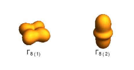
Figure 1: $\Gamma_{8(1)}$ and $\Gamma_{8(2)}$ orbitals with a similar structure as $d$-orbitals $d_{x^{2}-y^{2}}$ and $d_{3z^{2}-r^{2}}$, respectively.

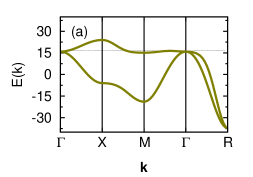
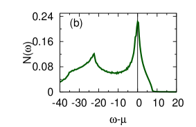
Figure 2: (a) Electron dispersions along high-symmetry direction $\Gamma$-X-M-$\Gamma$-R and (b) DOS, which is peaked near the Fermi level.

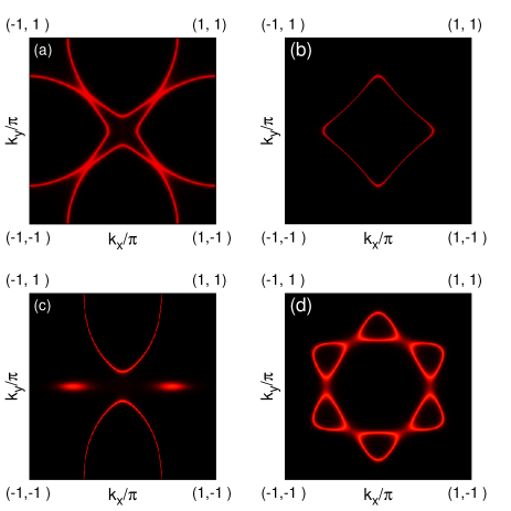
Figure 3: Electron dispersions along high-symmetry plane (a) (100), (b) at $\pi$ along (100), (c) (110) and (d) (111) obtained for the chemical potential $\mu$ = 16.4.

Kinetic energy after the Fourier transform can be expressed in terms of $\Gamma$ matrices defined as $\hat{\Gamma}^{0,1,2,3,4,5}=(\hat{\tau}_{0}\hat{\sigma}_{0},\hat{\tau}_{z}\hat{\sigma}_{0},\hat{\tau}_{x}\hat{\sigma}_{0},\hat{\tau}_{y}\hat{\sigma}_{x},\hat{\tau}_{y}\hat{\sigma}_{y},\hat{\tau}_{y}\hat{\sigma}_{z})$, where ${\sigma}_{i}$s and ${\tau}_{i}$s are Pauli’s matrices corresponding to the spin and orbital degrees of freedom, respectively. So that

$$\sum_{{\bf k}}\Psi^{\dagger}_{{\bf k}}H_{k}\Psi_{{\bf k}}=\sum_{{\bf k}}\sum_{i=0,1,..,5}\Psi^{\dagger}_{{\bf k}}d^{i}({\bf k})\Gamma^{i}\Psi_{{\bf k}}.$$ (3)

Here, $\Psi^{\dagger}_{{\bf k}}=(f^{\dagger}_{{\bf k}1\uparrow},f^{\dagger}_{{\bf k}2\uparrow},f^{\dagger}_{{\bf k}1\downarrow},f^{\dagger}_{{\bf k}2\downarrow})$ is the electron field with $d^{i}({\bf k})$s

$$d^{0}({\bf k}) = -\mu+8t\phi_{0}({\bf k})+\frac{28}{3}t^{\prime}\phi^{\prime}_{0}({\bf k})+\frac{128}{9}t^{\prime\prime}\phi^{\prime\prime}_{0}({\bf k})$$

$$d^{1}({\bf k}) = 4t\phi_{1}({\bf k})-\frac{2}{3}t^{\prime}\phi^{\prime}_{1}({\bf k})$$

$$d^{2}({\bf k}) = -4\sqrt{3}t\phi_{2}({\bf k})+\frac{2}{\sqrt{3}}t^{\prime}\phi^{\prime}_{2}({\bf k})$$

$$d^{3}({\bf k}) = \frac{16}{\sqrt{3}}t^{\prime}\phi^{\prime}_{3}({\bf k})+\frac{128}{9\sqrt{3}}t^{\prime\prime}\phi^{\prime\prime}_{3}({\bf k})$$

$$d^{4}({\bf k}) = \frac{16}{\sqrt{3}}t^{\prime}\phi^{\prime}_{4}({\bf k})+\frac{128}{9\sqrt{3}}t^{\prime\prime}\phi^{\prime\prime}_{4}({\bf k})$$

$$d^{5}({\bf k}) = \frac{16}{\sqrt{3}}t^{\prime}\phi^{\prime}_{5}({\bf k})+\frac{128}{9\sqrt{3}}t^{\prime\prime}\phi^{\prime\prime}_{5}({\bf k}).$$ (4)

$t^{\prime}$ and $t^{\prime\prime}$ are the second and third next-nearest neighbor hoping parameters. Various $\phi({\bf k})$s are expressed in terms of cosines and sines of the components of momentum in the Brillouin zone as

$$\phi_{0} = \cos k_{x}+\cos k_{y}+\cos k_{z}$$

$$\phi^{\prime}_{0} = \cos k_{y}\cos k_{z}+\cos k_{z}\cos k_{x}+\cos k_{x}\cos k_{y}$$

$$\phi_{1} = \cos k_{x}+\cos k_{y}-2\cos k_{z}$$

$$\phi^{\prime}_{1} = \cos k_{y}\cos k_{z}+\cos k_{z}\cos k_{x}-2\cos k_{x}\cos k_{y}$$

$$\phi_{2} = \cos k_{x}-\cos k_{y}$$

$$\phi^{\prime}_{2} = \cos k_{y}\cos k_{z}-\cos k_{z}\cos k_{x}$$

$$\phi^{\prime}_{3} = \sin k_{y}\sin k_{z}$$

$$\phi^{\prime}_{4} = \sin k_{z}\sin k_{x}$$

$$\phi^{\prime}_{5} = \sin k_{x}\sin k_{y}$$

$$\phi^{\prime\prime}_{0} = \cos k_{x}\cos k_{y}\cos k_{z}$$

$$\phi^{\prime\prime}_{3} = \cos k_{x}\sin k_{y}\sin k_{z}$$

$$\phi^{\prime\prime}_{4} = \sin k_{x}\cos k_{y}\sin k_{z}$$

$$\phi^{\prime\prime}_{5} = \sin k_{x}\sin k_{y}\cos k_{z}.$$ (5)

In the absence of the second and third nearest-neighbor hopping, the kinetic part of the Hamiltonian reduces to that of manganitesdagotto with the only difference of a constant multiplication factor. In the following, the unit of energy is set to be $t$. Calculated electron dispersions for $t^{\prime}=-0.38$ and $t^{{\prime}{\prime}}=0.18$, which consists of doubly degenerate eigenvalues, are shown in Fig. 3(a) along the high symmetry directions. A large hole pocket near X and the extrema exhibited by two bands near $\Gamma$ just below the Fermi level are broadly in agreement with 4$f$ dominated part in the band-structure calculations. The density of states (DOS) show two peaks with larger one being in the vicinity of the Fermi level (Fig. 3(b)). It is not unexpected particularly because of the flatness of the two bands near $\Gamma$ contributing mostly to the DOS at the Fermi level. Interestingly, a hot spot near $\Gamma$ has been observed also in the ARPES measurements, which points towards the possibility of strong ferromagnetic fluctuations.neupane Here, the chemical potential is chosen to be 16.4 to obtain a better agreement with the ARPES FSs.

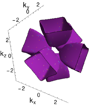
Figure 4: Fermi surfaces in the Brillouin zone for the chemical potential $\mu$ = 16.4.

Fig. 3 shows FSs cut along different high-symmetry planes. It has an ellipse-like structure with major axis aligned along $\Gamma$-X for the (100) plane while touching each other along $\Gamma$-M direction. On the other hand, the parallel plane at (0, 0, $\pi$) consists of a single squarish pocket around that point. In the absence of four-fold rotation symmetry for the (110) plane, two large ellipse-like FSs surfaces are present with the major axes along $\Gamma$-Y direction while small pockets exist along $\Gamma$-X direction. The six-fold rotation symmetry is reflected by the six pockets along (111) plane. All of them are obtained from the FSs shown in the whole Brillouin zone as in the Fig. 3. It consists of an ellipsoid-like FSs with largest semi-principal axes coinciding with $\Gamma$-X, however, with a squarish cross section. An overall good agreement exists with the several recent ARPES measurements.koitzsch ; neupane ARPES estimates are believed to more reliable when compared with the earlier estimates from dHvA experiments carried out in the presence of magnetic field as the latter has the potential to affect the hot spots.

III Multipolar susceptibilities

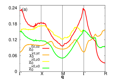
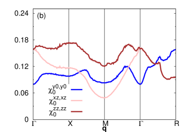
Figure 5: (a) Magnetic and quadrupolar static susceptibilities along high-symmetry direction $\Gamma$-X-M-$\Gamma$-R. (b) Octapolar static susceptibilities.

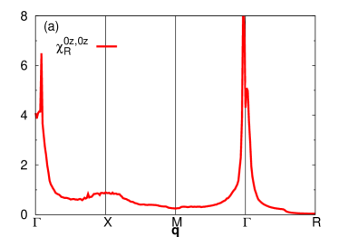
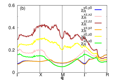
Figure 6: Multipolar static susceptibilities calculated at the RPA-level for $U=15$ and $J=0.16U$. (a) Spin susceptibility diverges near (0, 0, 0). (b) For the same set of interaction parameters quadrupolar and octapolar susceptibilities are divergenceless.

Sixteen multipolar moments can be defined for the $\Gamma_{8}$ state including one charge, three dipole, five quadrupole and seven octapole, which are rank-0, rank-1, rank-2 and rank-3 tensors, respectively. The dipole belongs to the $\Gamma^{-}_{4}$ irreducible representation, where $-$ sign denote the breaking of time reversal symmetry. It’s components are given by the outer product of Pauli’s matrices $\hat{\tau_{0}}\hat{\sigma_{i}}$s. The quadrupole moments belonging to $\Gamma^{+}_{3}$ are $\hat{\tau_{x}}\hat{\sigma_{0}}$ and $\hat{\tau_{z}}\hat{\sigma_{0}}$ while those belonging to $\Gamma^{+}_{5}$ irreducible representations are expressed as $\hat{\tau_{i}}\hat{\sigma_{y}}$s. The octapular moments with $\Gamma^{-}_{2}$ representation is $\hat{\tau_{y}}\hat{\sigma_{0}}$, whereas the $z$-component of those belonging to $\Gamma^{-}_{4}$ and $\Gamma^{-}_{5}$ are $2\hat{\tau_{z}}\hat{\sigma_{z}}$ and $2\hat{\tau_{x}}\hat{\sigma_{z}}$, respectively.

In order to examine the multipolar ordering instabilities, we calculate susceptibilities while considering only the $z$-component whenever component along three coordinate axes are present as that will be sufficient because of the cubic symmetry. Multipolar susceptibilities are defined astakimoto1

$${\chi}^{pq,rs}({\bf q},i\omega_{n})=\frac{1}{\beta}\int^{\beta}_{0}{d\tau e^{i\omega_{n}\tau}\langle T_{\tau}[{\cal O}^{pq}_{{\bf q}}(\tau){\cal O}^{rs}_{-{\bf q}}(0)]\rangle},$$ (6)

where

$${\cal O}^{pq}_{{\bf q}}=\sum_{\bf k}\sum_{\sigma\sigma^{\prime}}\sum_{\mu\mu^{\prime}}f^{\dagger}_{\mu\sigma}({\bf k}+{\bf q})\tau^{p}_{\mu\mu^{\prime}}\sigma^{q}_{\sigma\sigma^{\prime}}f_{\mu^{\prime}\sigma^{\prime}}({\bf k}).$$ (7)

They can be expressed in terms of

$$\chi^{\sigma_{1}\sigma_{2};\sigma_{4}\sigma_{3}}_{\mu_{1}\mu_{2};\mu_{4}\mu_{3}}({\bf q},i\omega_{n}) = \frac{1}{\beta}\int^{\beta}_{0}d\tau\sum_{{\bf k},{\bf k}^{\prime}}\langle T_{\tau}f^{\dagger}_{{\bf k}+{\bf q}\mu_{1}\sigma_{1}}(\tau)f_{{\bf k}\mu_{2}\sigma_{2}}(\tau)$$ (8)

$$\times f^{\dagger}_{{\bf k}^{\prime}-{\bf q}^{\prime}\mu_{3}\sigma_{3}}(0)f_{{\bf k}^{\prime}\mu_{4}\sigma_{4}}(0)\rangle$$

which form a 16$\times$16 matrix. Thus, the dipole or spin susceptibility is given by

$${\chi}^{0z,0z}({\bf q},i\omega_{n})=\sum_{\sigma\sigma^{\prime}}\sum_{\mu\mu^{\prime}}\sigma\sigma^{\prime}\chi^{\sigma\sigma;\sigma^{\prime}\sigma^{\prime}}_{\mu\mu;\mu^{\prime}\mu^{\prime}}({\bf q},i\omega_{n}),$$ (9)

where $\sigma$ and $\mu$ in front of $\chi$ takes +1 or -1 corresponding to the two spin or orbital degrees of freedom. Various quadrupolar and octapolar susceptibilities are given as

$${\chi}^{x0,x0}({\bf q},i\omega_{n}) = \sum_{\sigma}\sum_{\mu\mu^{\prime}}\chi^{\sigma\sigma;\sigma\sigma}_{\mu\bar{\mu};\mu^{\prime}\bar{\mu}^{\prime}}({\bf q},i\omega_{n})$$

$${\chi}^{z0,z0}({\bf q},i\omega_{n}) = \sum_{\sigma}\sum_{\mu\mu^{\prime}}\mu\mu^{\prime}\chi^{\sigma\sigma;\sigma\sigma}_{\mu\mu;\mu^{\prime}\mu^{\prime}}({\bf q},i\omega_{n})$$

$${\chi}^{yz,yz}({\bf q},i\omega_{n}) = -i^{2}\sum_{\sigma\sigma^{\prime}}\sum_{\mu\mu^{\prime}}\sigma\sigma^{\prime}\mu\mu^{\prime}\chi^{\sigma\sigma;\sigma^{\prime}\sigma^{\prime}}_{\mu\bar{\mu};\mu^{\prime}\bar{\mu}^{\prime}}({\bf q},i\omega_{n})$$

and

$${\chi}^{y0,y0}({\bf q},i\omega_{n}) = -i^{2}\sum_{\sigma}\sum_{\mu\mu^{\prime}}\mu\mu^{\prime}\chi^{\sigma\sigma;\sigma\sigma}_{\mu\bar{\mu};\mu^{\prime}\bar{\mu}^{\prime}}({\bf q},i\omega_{n})$$

$${\chi}^{xz,xz}({\bf q},i\omega_{n}) = \sum_{\sigma\sigma^{\prime}}\sum_{\mu\mu^{\prime}}\sigma\sigma^{\prime}\chi^{\sigma\sigma;\sigma^{\prime}\sigma^{\prime}}_{\mu\bar{\mu};\mu^{\prime}\bar{\mu}^{\prime}}({\bf q},i\omega_{n})$$

$${\chi}^{zz,zz}({\bf q},i\omega_{n}) = \sum_{\sigma\sigma^{\prime}}\sum_{\mu\mu^{\prime}}\sigma\sigma^{\prime}\mu\mu^{\prime}\chi^{\sigma\sigma;\sigma^{\prime}\sigma^{\prime}}_{\mu\mu;\mu^{\prime}{\mu}^{\prime}}({\bf q},i\omega_{n}),$$ (11)

respectively.

Fig. 5 shows different static multipolar susceptibilities with well-defined peaks for some while broad hump like structure for the other. Particularly, the spin susceptibility $\bar{\chi}^{0z,0z}$ is, among all, sharply peaked, however, at $\approx$ ${\bf Q}_{3}$ = (0, 0, 0). Quadrupolar susceptibility $\bar{\chi}^{yz,yz}$ corresponding to the AFQ order observed in experiments, on the other hand, does shows a peak near ${\bf Q}_{1}$. Other quadrupolar susceptibility $\bar{\chi}^{x0,x0}$ is peaked near $\approx$ ${\bf Q}_{3}$ while $\bar{\chi}^{z0,z0}$ has a broad hump like structure near ($\pi,0,0$) and a peak slightly away from ($\pi/2,\pi/2,\pi/2$). We further note that $\bar{\chi}^{x0,x0}=\bar{\chi}^{xz,xz}$, $\bar{\chi}^{y0,y0}=\bar{\chi}^{yz,yz}$ and $\bar{\chi}^{z0,z0}=\bar{\chi}^{zz,zz}$ as shown in Fig. 5(b)

IV Multipolar susceptibilities in the presence of interaction

In order to investigate the role of electron-electron correlation, we consider the standard onsite Coulomb interaction terms given as

$$\mathcal{H}_{int} = U\sum_{{\bf i},\mu}n_{{\bf i}\mu\uparrow}n_{{\bf i}\mu\downarrow}+(U^{\prime}-\frac{J}{2})\sum_{{\bf i},\mu<\nu}n_{{\bf i}\mu}n_{{\bf i}\nu}$$

$$- 2J\sum_{{\bf i},\mu<\nu}{\bf{S_{{\bf i}\mu}}}\cdot{\bf{S_{{\bf i}\nu}}}+J\sum_{{\bf i},\mu<\nu,\sigma}f_{{\bf i}\mu\sigma}^{\dagger}f_{{\bf i}\mu\bar{\sigma}}^{\dagger}f_{{\bf i}\nu\bar{\sigma}}f_{{\bf i}\nu\sigma},$$

(12)

in a manner similar to the various correlated multiorbital systems. First term represents the intraorbital Coulomb interaction for each orbital. Second and third term represent the density-density interaction and Hund’s coupling between the two orbitals. Fourth term represents the pair-hopping energy whereas the condition $U^{\prime}$ = $U$ - $2J$ is essential for the rotational invariance.

Multipolar susceptibilities in the presence of interaction can be obtained from Dyson’s equation yielding

$$\hat{\chi}_{R}({\bf q},i\omega)=(\hat{{\bf 1}}-\hat{U}\hat{{\chi}}({\bf q},i\omega))^{-1}\hat{{\chi}}({\bf q},i\omega).$$ (13)

Here, $\hat{{\bf 1}}$ is a $16\times 16$ identity matrix, whereas the interaction matrix is given byscherer

$${U}^{\sigma_{1}\sigma_{2};\sigma_{3}\sigma_{4}}_{\mu_{1}\mu_{2};\mu_{3}\mu_{4}}$$

$$=\left\{\begin{array}[]{@{\,} l @{\,} c}-U&(\mu_{1}=\mu_{2}=\mu_{3}=\mu_{4},\sigma_{1}=\sigma_{2}\neq\sigma_{3}=\sigma_{4})\\ -U^{\prime}&(\mu_{1}=\mu_{2}\neq\mu_{3}=\mu_{4},\sigma_{1}=\sigma_{2}\neq\sigma_{3}=\sigma_{4})\\ -J&(\mu_{1}=\mu_{4}\neq\mu_{2}=\mu_{3},\sigma_{1}=\sigma_{2}\neq\sigma_{3}=\sigma_{4})\\ -J^{\prime}&(\mu_{1}=\mu_{3}\neq\mu_{2}=\mu_{4},\sigma_{1}=\sigma_{2}\neq\sigma_{3}=\sigma_{4})\\ -(U-J^{\prime})&(\mu_{1}=\mu_{2}\neq\mu_{3}=\mu_{4},\sigma_{1}=\sigma_{2}=\sigma_{3}=\sigma_{4})\\ (U-J^{\prime})&(\mu_{1}=\mu_{4}\neq\mu_{2}=\mu_{3},\sigma_{1}=\sigma_{2}=\sigma_{3}=\sigma_{4})\\ U&(\mu_{1}=\mu_{2}=\mu_{3}=\mu_{4},\sigma_{1}=\sigma_{4}\neq\sigma_{2}=\sigma_{3})\\ U^{\prime}&(\mu_{1}=\mu_{4}\neq\mu_{2}=\mu_{3},\sigma_{1}=\sigma_{4}\neq\sigma_{2}=\sigma_{3})\\ J&(\mu_{1}=\mu_{2}\neq\mu_{3}=\mu_{4},\sigma_{1}=\sigma_{4}\neq\sigma_{2}=\sigma_{3})\\ J^{\prime}&(\mu_{1}=\mu_{3}\neq\mu_{2}=\mu_{4},\sigma_{1}=\sigma_{4}\neq\sigma_{2}=\sigma_{3})\\ 0&(\mathrm{otherwise})\end{array}\right..$$ (25)

Fig. 6 show the multipolar static susceptibilities at the RPA-level. As expected, the RPA spin susceptibility requires the smallest critical interaction strength $U=15$ ($U$/$W$ $<1/3$) with $J=0.16U$ to show the divergence. Interestingly, it diverges near ${\bf Q}_{3}$ instead of at the AFM ordering wave vector ${\bf Q}_{2}$, which is not surprising because there exists a large DOS near $\Gamma$ that leads also to the peak near ${\bf Q}_{3}$ in bare spin suspceptibility. Thus, AFQ instability corresponding to the $\Gamma^{+}_{5}$ representation is absent in the model despite the bare quadurpole susceptibility being peaked near ${\bf Q}_{1}$. However, we believe that the strong low-energy ferromagnetic fluctuations in the paramagnetic phase may have important implications for the persistent ferromagnetic correlations in various ordered phases as observed by various experiments.demishev2 ; jang

V Conclusions and discussions

In conclusions, we have described a tight-binding model with the bases as $\Gamma_{8}$, which captures the salient features of the Fermi surfaces along the high-symmetry planes as observed in the ARPES measurements. A large density of state is obtained near the Fermi level due to the flatness of the bands close to $\Gamma$, which bears a remarkable similarity to the hot-spot observed in another ARPES experiments. Multipolar susceptibilities calculated with the standard onsite Coulomb interactions as in other multiorbital systems show that it is the spin susceptibility that exhibits strongest diverging behavior. Moreover, it does so in the low-momentum region implying an underlying ferromagnetic instability.

It is clear that nature of the instability obtained with the realistic electronic structure is different from the actual order in CeB₆. However, it is important to note that some of the recent experiments have provided the evidence of strong ferromagnetic correlations in the ordered phases. For instance, there exists magnetic spin resonance in the AFQ phase, which has been attributed to the FM correlations. Further, the most intense spin-wave excitation modes have been observed at zero-momentum instead of the AFM ordering wavevector by the INS measurements in the coexistence phase, which continues to be present even in the AFQ phase. A similar INS measurement in the paramagnetic phase is highly desirable to probe the existence of ferromagnetic correlations in the paramagnetic phase. So far only an indirect indication in the form of hot-spot observed by ARPES near $\Gamma$ is available. In order to understand above mentioned features, we believe that the strong low-energy ferromagnetic fluctuations obtained within the two-orbital model with the realistic electronic structure may be an important step. To explain AFQ and other multipole order, it would perhaps be necessary to include the local-exchange terms involving AFQ and multipolar moments. Such a proposal should be the subject matter of future investigation in order to describe various complex ordering phenomena as well as associated unusual features within a single model.

We acknowledge the use of HPC clusters at HRI.

References

- (1) J. A. Mydosh and P. M. Oppeneer, Colloquium: hidden order, superconductivity, and magnetism-the unsolved case of URu2Si2, Rev. Mod. Phys. 83, 1301 (2011).
- (2) P. Thalmeier, T. Takimoto, J. Chang, and I. Eremin, J. Phys. Soc. Jpn. 77, 43 (2008).
- (3) Y. Kuramoto, H. Kusunose, and A. Kiss, J. Phys. Soc. Jpn. 78, 072001 (2009).
- (4) P. Santini, Rev. Mod. Phys. 81, 807 (2009).
- (5) T. Takimoto, J. Phys. Soc. Jpn. 80 123710 (2011).
- (6) T. Kasuya, K. Takegahara, Y. Aoki, T. Suzuki, S. Kunii, M. Sera, N. Sato, T. Fujita., T. Goto., A. Tamaki, and T. Komatsubara, in: Proc. Intern, Conf. on Valence Instabili- ties, eds. P. Wachter and H. Boppart, 359 (North-Holland. Amsterdam, 1982).
- (7) J. M. Effantin, J. Rossat-Mignod, P. Burlet, H. Bartholin, S. Kunni and T. Kasuya, J. Magn. Magn. Mater. 4748 145–148 (1985).
- (8) R. G. Goodrich, D. P. Young, D. Hall, L. Balicas, Z. Fisk, N. Harrison, J. Betts, A. Migliori, F. M. Woodward, and J. W. Lynn, Phys. Rev. B 69, 054415 (2004).
- (9) T. Matsumura, T. Yonemura, K. Kunimori, M. Sera, F. Iga, T. Nagao, and J.-I Igarashi, Phys. Rev. B 85, 174417 (2012).
- (10) R. Shiina, H. Shiba, P. Thalmeier, A. Takahashi, and O. Sakai, J. Phys. Soc. Jpn. 72, 1216 (2003).
- (11) P. Thalmeier, R. Shiina, H. Shiba, A. Takahashi, and O. Sakai, J. Phys. Soc. Jpn. 72, 3219 (2003).
- (12) O. Zaharko, P. Fischer, A. Schenck, S. Kunii, P.-J. Brown, F. Tasset, and T. Hansen, Phys. Rev. B 68, 214401 (2003).
- (13) S. V. Demisheva, A. V. Semenoa, A. V. Bogacha, Yu. B. Padernob, N. Yu. Shitsevalovab, N. E. Sluchankoa, J. Magn. Magn. Mater. 300, e534-e537 (2006).
- (14) S. V. Demishev, A. V. Semeno, A. V. Bogach, N. A. Samarin, T. V. Ishchenko, V. B. Filipov, N. Yu. Shitsevalova, and N. E. Sluchanko, Phys. Rev. B 80, 245106 (2009).
- (15) C. Krellner, T. Förster, H. Jeevan, C. Geibel, and J. Sichelschmidt, Phys. Rev. Lett. 100, 066401 2008.
- (16) P. Schlottmann, Phys. Rev. B 86, 075135 (2012).
- (17) J. Sichelschmidt, J. Wykhoff, H.-A. Krug von Nidda, I. I. Fazlishanov, Z. Hossain, C. Krellner, C. Geibel, and F. Steglich, J. Phys.: Condens. Matter 19, 016211 (2007).
- (18) E. M. Bruning, C. Krellner, M. Baenitz, A. Jesche, F. Steglich, and C. Geibel, Phys. Rev. Lett. 101, 117206 (2008).
- (19) G. Friemel, Y. Li, A. V. Dukhnenko, N. Y. Shitsevalova, N. E. Sluchanko, A. Ivanov, V. B. Filipov, B. Keimer, and D.S. Inosov, Nat. Comm. 3, 830 (2012).
- (20) H. Jang, G. Friemel, J. Ollivier, A. V. Dukhnenko, N. Yu. Shitsevalova, V. B. Filipov, B. Keimer, and D. S. Inosov, Nat. Mat. 13, 682 (2014).
- (21) F. J. Okhawa, J. Phys. Soc. Jpn. 54, 3909 (1985).
- (22) N. Harrison, P. Meson, P.-A. Probst, and M. Springford, J . Phys.: Condens. Matter 5 7435 (1993).
- (23) S. Nakamura, T. Goto, and S. Kunii, J. Phys. Soc. Jpn. 64, 3941 (1995).
- (24) I. Eremin, G. Zwicknagl, P. Thalmeier, and P. Fulde, Phys. Rev. Lett. 101, 187001 (2008).
- (25) A. Akbari and P. Thalmeier, Phys. Rev. Lett. 108, 146403 (2012).
- (26) A. Koitzsch, N. Heming, M. Knupfer, B. Bchner, P. Y. Portnichenko, A. V. Dukhnenko, N. Y. Shitsevalova, V. B. Filipov, L. L. Lev, V. N. Strocov, J. Ollivier, and D. S. Inosov, Nat. Comm. 7 10876 (2016).
- (27) M. Neupane, N. Alidoust, I. Belopolski, G. Bian, S.-Y. Xu, Dae-Jeong Kim, P. P. Shibayev, D. S. Sanchez, H. Zheng, T.-R. Chang, H.-T. Jeng, P. S. Riseborough, H. Lin, A. Bansil, T. Durakiewicz, Z. Fisk, and M. Z. Hasan, Phys. Rev. B 92, 104420 (2015).
- (28) Y. Ōnuki, T. Komatsubara, P. H. P. Reinders, and M. Springford, J. Phys. Soc. Jpn. 58, 3698 (1989).
- (29) T. Kasuya and H. Harima, J. Phys. Soc. Jpn. 65, 3698 (1996).
- (30) M. B. Suvasini, G. Y. Guo, W. M. Temmerman, G. A. Gehring, and M. Biasini, J. Phys.: Condens. Matter 8 7105-7125 (1996).
- (31) N. Singh, S. M. Saini, T. Nautiyal and S. Auluck, J. Phys.: Condens. Matter 19 (2007) 346226.
- (32) T. Hotta and K. Ueda, Phys. Rev. B 67, 104518 (2003).
- (33) E. Dagotto, T. Hotta, and A. Moreoa, Phys. Rep. 344 1 (2001).
- (34) T. Takimoto, T. Hotta, T. Maehira, and K. Ueda, J. Phys.: Condens. Matter 14 (2002) L369-L375.
- (35) D. D. Scherer, I. Eremin, and B. M. Andersen, Phys. Rev. B 94, 180405 (2016).