Guided Deep List: Automating the Generation of Epidemiological Line Lists from Open Sources

Abstract

Real-time monitoring and responses to emerging public health threats rely on the availability of timely surveillance data. During the early stages of an epidemic, the ready availability of line lists with detailed tabular information about laboratory-confirmed cases can assist epidemiologists in making reliable inferences and forecasts. Such inferences are crucial to understand the epidemiology of a specific disease early enough to stop or control the outbreak. However, construction of such line lists requires considerable human supervision and therefore, difficult to generate in real-time. In this paper, we motivate Guided Deep List, the first tool for building automated line lists (in near real-time) from open source reports of emerging disease outbreaks. Specifically, we focus on deriving epidemiological characteristics of an emerging disease and the affected population from reports of illness. Guided Deep List uses distributed vector representations (ala word2vec) to discover a set of indicators for each line list feature. This discovery of indicators is followed by the use of dependency parsing based techniques for final extraction in tabular form. We evaluate the performance of Guided Deep List against a human annotated line list provided by HealthMap corresponding to MERS outbreaks in Saudi Arabia. We demonstrate that Guided Deep List extracts line list features with increased accuracy compared to a baseline method. We further show how these automatically extracted line list features can be used for making epidemiological inferences, such as inferring demographics and symptoms-to-hospitalization period of affected individuals.

1 Introduction

An epidemiological line list [1, 2] is a listing of individuals suffering from a disease that describes both their demographic details as well as the timing of clinically and epidemiologically significant events during the course of disease. These are typically used during outbreak investigations of emerging diseases to identify key features, such as incubation period, symptoms, associated risk factors, and outcomes. The ultimate goal is to understand the disease well enough to stop or control the outbreak. Ready availability of line lists can also be useful in contact tracing as well as risk identification of spread such as the spread of Middle Eastern Respiratory Syndrome (MERS) in Saudi Arabia or Ebola in West Africa.

Formats of line lists are generally dependent on the kind of disease being investigated. However, some interesting features that are common for most formats include demographic information about cases. Demographic information can include age, gender, and location of infection. Depending on the disease being investigated, one can consider other addendums to this list, such as disease onset features (onset date, hospitalization date and outcome date) and clinical features (comorbidities, secondary contact, animal contact).

Traditionally, line lists have been curated manually and have rarely been available to epidemiologists in near-real time. Our primary objective is to automatically generate line lists of emerging diseases from open source reports such as WHO bulletins [3] and make such lists readily available to epidemiologists. Previous work [1, 2] has shown the utility in creating such lists through labor intensive human curation. We now seek to automate much of this effort. To the best of our knowledge, our work is the first to automate the creation of line lists.

Figure 1: Tabular extraction of line list by Guided Deep List given a textual block of a WHO MERS bulletin. Each row in the extracted table depicts an infected case (or, patient) and columns represent the epidemiological features corresponding to each case. Information for each case in the table is then used to make epidemiological inferences, such as inferring demographic distribution of cases

The availability of massive textual public health data coincides with recent developments in text modeling, including distributed vector representations such as word2vec [4, 5] and doc2vec [6]. These neural network based language models when trained over a representative corpus convert words to dense low-dimensional vector representations, most popularly known as word embeddings. These word embeddings have been widely used with considerable accuracy to capture linguistic patterns and regularities, such as vec(Paris) - vec(France) $\approx$ vec(Madrid) - vec(Spain) [7, 8]. A second development relevant for line list generation pertains to semantic dependency parsing, which has emerged as an effective tool for information extraction, e.g., in an open information extraction context [9], Negation Detection [10, 11, 12], relation extraction [13, 14] and event detection [15]. Given an input sentence, dependency parsing is typically used to extract its semantic tree representations where words are linked by directed edges called dependencies.

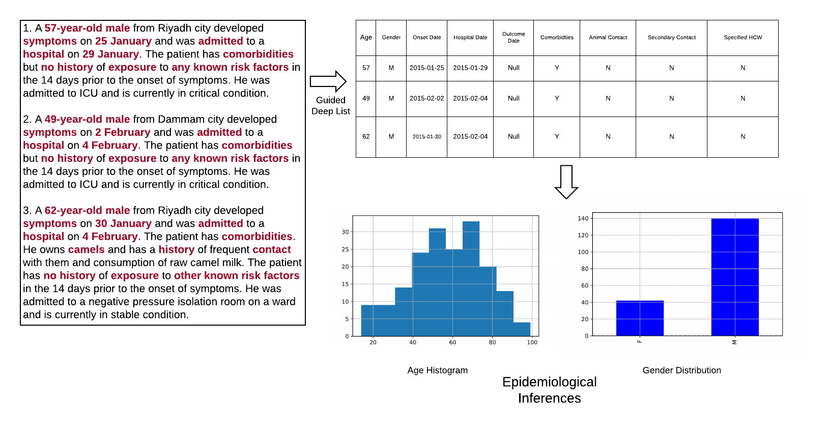
Building upon these techniques, we formulate Guided Deep List, a novel framework for automatic extraction of line list from WHO bulletins [3]. Guided Deep List is guided in the sense that the user provides a seed indicator (or, keyword) for each line list feature to guide the extraction process. Guided Deep List uses neural word embeddings to expand the seed indicator and generate a set of indicators for each line list feature. The set of indicators is subsequently provided as input to dependency parsing based shortest distance and negation detection approaches for extracting line list features. As can be seen in Figure 1, Guided Deep List takes a WHO bulletin as input and outputs epidemiological line list in tabular format where each row represents a line list case and each column depicts the features corresponding to each case. The extracted line list provides valuable information to model the epidemic and understand the segments of population who would be affected.

Our main contributions are as follows.
$\>\bullet$ Automated: Guided Deep List is fully automatic, requiring no human intervention.
$\>\bullet$ Novelty: To the best of our knowledge, there has been no prior systematic efforts at tabulating such information automatically from publicly available health bulletins.
$\>\bullet$ Real-time: Guided Deep List can be deployed for extracting line list in a (near) real-time setting.
$\>\bullet$ Evaluation: We present a detailed and prospective analysis of Guided Deep List by evaluating the automatically inferred line list against a human curated line list for MERS outbreaks in Saudi Arabia. We also compare Guided Deep List against a baseline method.
$\>\bullet$ Epidemiological inferences: Finally, we also demonstrate some of the utilities of real-time automated line listing, such as inferring the demographic distribution and symptoms-to-hospitalization period.

2 Problem Overview

In this manuscript, we intend to focus on Middle Eastern Respiratory Syndrome (MERS) outbreaks in Saudi Arabia [2] (2012-ongoing) as our case study. MERS was a relatively less understood disease when these outbreaks began. Therefore, MERS was poised as an emerging outbreak leading to good bulletin coverage about the infectious cases individually. This makes these disease outbreaks ideally suited to our goals. MERS is infectious as well and animal contact has been posited as one of the transmission mechanisms of the disease. For each line list case, we seek to extract automatically three types of epidemiological features as follows. (a) Demographics: Age and Gender, (b) Disease onset: onset date, hospitalization date and outcome date and (c) Clinical features: animal contact, secondary contact, comorbidities and specified healthcare worker (abbreviated as HCW).

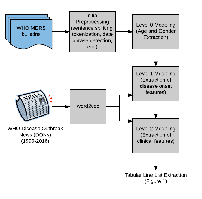
In Figure 2, we show all the internal components comprising the framework of Guided Deep List. Guided Deep List takes multiple WHO MERS bulletins as input. The textual content of each bulletin is pre-processed by sentence splitting, tokenization, lemmatization, POS tagging, and date phrase detection using spaCy [16] and BASIS Technologies’ Rosette Language Processing (RLP) tools [17]. The pre-processing step is followed by three levels of modeling as follows. (a) Level 0 Modeling for extracting demographic information of cases, such as age and gender. In this level, we also identify the key sentences related to each line list case, (b) level 1 Modeling for extracting disease onset information and (c) level 2 Modeling for extracting clinical features. This is the final level of modeling in Guided Deep List framework. Features extracted at this level are associated with two labels: Y or N. Therefore, modeling at this level combines neural word embeddings with dependency parsing-based negation detection approaches to classify the clinical features into Y or N. In the subsequent section, we will discuss each internal component of Guided Deep List in detail.

Figure 2: Block diagram depicting all components of the Guided Deep List framework. Given multiple WHO MERS bulletins as input, these components function in the depicted order to extract line lists in tabular form)

3 Guided Deep List

Given multiple WHO MERS bulletins as input, Guided Deep List proceeds through three levels of modeling for extracting line list features. We describe each level in turn.

3.1 Level O Modeling

In level 0 modeling, we extract the age and gender for each line list case. These two features are mentioned in a reasonably structured way and therefore, can be extracted using a combination of regular expressions as shown in Algorithm 1. One of the primary challenges in extracting line list cases is the fact that a single WHO MERS bulletin can contain information about multiple cases. Therefore, there is a need to distinguish between cases mentioned in the bulletin. In level 0 modeling, we make use of the age and gender extraction to also identify sentences associated with each case. Since age and gender are the fundamental information to be recorded for a line list case, we postulate that the sentence mentioning the age and gender will be the starting sentence describing a line list case (see the textual block in Figure 1). Therefore, the number of cases mentioned in the bulletin will be equivalent to the number of sentences mentioning age and gender information. We further postulate that information related to the other features (disease onset or critical) will be present either in the starting sentence or the sentences subsequent to the starting one not mentioning any age and gender related information ((see the textual block in Figure 1)). For more details on level 0 modeling, please see Algorithm 1. In Algorithm 1, $\mathcal{N}$ represents the number of line list cases mentioned in the bulletin and $\mathcal{SC}_{n}$ represents the set of sentences mentioning the $n^{th}$ case.

Input : set of sentences in the input WHO MERS bulletin

Output : Age and Gender for each line list case, index of the starting sentence for each case

1 n = 0;

2 $\mathcal{SC}_{n}$ = Null;

3 $\mathcal{R}_{1}$ = \s+(?P<age>\d{1,2})(.{0,20})(\s+|-)(?P<gender>woman|man|male|female|boy|girl|housewife);

4

5$\mathcal{R}_{2}$ = \s+(?P<age>\d{1,2})\s*years?(\s|-)old;

6

7$\mathcal{R}_{3}$ = \s*(?P<gender>woman|man|male|female|boy|girl|housewife|he|she);

8 for each sentence in the bulletin do

9       is-starting $\rightarrow$ 0;

10       if $\mathcal{R}_{1}$.match(sentence) then

11             Age = int($\mathcal{R}_{1}$.groupdict()[’age’]);

12             Gender = $\mathcal{R}_{1}$.groupdict()[’gender’];

13             is-starting $\rightarrow$ 1;

14            

15      else

16             if $\mathcal{R}_{2}$.match(sentence) then

17                   Age = int($\mathcal{R}_{3}$.groupdict()[’age’]);

18                  

19            else

20                   Age = Null;

21                  

22            if $\mathcal{R}_{3}$.match(sentence) then

23                   Gender = int($\mathcal{R}_{3}$.groupdict()[’gender’]);

24                  

25            else

26                   Gender = Null;

27                  

28            if Age $\neq$ Null $\&\&$ Gender $\neq$ Null then

29                   is-starting $\rightarrow$ 1;

30                  

31            

32      if is-starting then

33             n += 1;

34             $\mathcal{SC}_{n}$ = index of the sentence;

35            

36      

$\mathcal{N}$ = n;

Algorithm 1 Level 0 modeling

3.2 WHO Template Learning

Before presenting the details of level 1 modeling and level 2 modeling, we will briefly discuss the WHO template learning process which provides word embeddings as input to both these levels of modeling (see Figure 2). In the template learning process, our main objective is to identify words which tend to share similar contexts or appear in the contexts of each other specific to the WHO bulletins (contexts of a word refer to the words surrounding it in a specified window size). For instance, consider the sentences $\mathcal{S}_{1}=$The patient had no contact with animals and $\mathcal{S}_{2}=$The patient was supposed to have no contact with camels. The terms animals and camels appear in similar contexts in both $\mathcal{S}_{1}$ and $\mathcal{S}_{2}$. Both the terms animals and camels are indicative of information pertaining to patient’s exposure to animals or animal products.

Similarly, consider the sentences $\mathcal{S}_{3}=$The patient had an onset of symptoms on 23rd January 2016 and $\mathcal{S}_{4}=$The patient developed symptoms on 23rd January 2016. The terms onset and symptoms are indicators for the onset date feature and both of them appear in similar contexts or contexts of each other in $\mathcal{S}_{3}$ and $\mathcal{S}_{4}$.

For the template learning process, neural network inspired word2vec models are ideally suited to our goals because these models work on the hypothesis that words sharing similar contexts or tending to appear in the contexts of each other have similar embeddings. In recent years, word2vec models based on the skip-gram architectures [4, 5] have emerged as the most popular word embedding models for information extraction tasks [18, 19, 20]. We used two variants of skip-gram models: (a) the skip-gram model trained using the negative sampling technique (SGNS [5]) and (b) the skip-gram model trained using hierarchical sampling (SGHS [5]) to generate embeddings for each term in the WHO vocabulary $\mathcal{W}$. $\mathcal{W}$ refers to the list of all unique terms extracted from the entire corpus of WHO Disease Outbreak News (DONs) corresponding to all diseases downloaded from http://www.who.int/csr/don/archive/disease/en/. The embeddings for each term in $\mathcal{W}$ were provided as input to level 1 modeling and level 2 modeling as shown in Figure 2.

3.3 Level 1 Modeling

The level 1 modeling is responsible for extracting the disease onset features, such as symptom onset date, hospitalization date and outcome date for each linelist case, say the $n^{th}$ case. For extracting a given disease onset feature, the level 1 modeling takes three inputs: (a) seed indicator for the feature, (b) the word embeddings generated using SGNS or SGHS for each term in the WHO vocabulary $\mathcal{W}$ and (c) $\mathcal{SC}_{n}$ representing the set of sentences describing the $n^{th}$ case for which we are extracting the feature.

Growth of seed indicator

In the first phase of level 1 modeling, we discover the top-$K$ similar (or, closest) indicators in the embedding space to the seed indicator for each feature. The similarity metric used is the standard cosine similarity metric. Therefore, we expand the seed indicator to create a set of $K+1$ indicators for each feature. In Table 1 we show the indicators discovered by SGNS for each disease onset feature given the seed indicators as input.

Table 1: Seed indicator and the discovered indicators using word embeddings generated by SGNS

Features	Seed indicator	Discovered indicators
Onset date	onset	symptoms, symptom, prior, days, dates
Hospitalization date	hospitalized	admitted, screened, hospitalised, passed, discharged
Outcome date	died	recovered, passed, became, ill, hospitalized

Shortest Dependency Distance

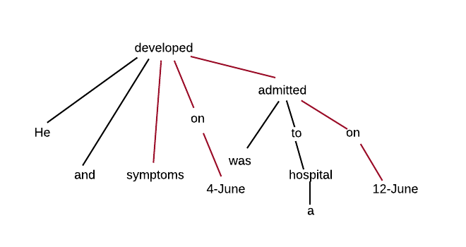
In the second phase, we use these $K+1$ indicators to extract the disease onset features. For each indicator $\mathcal{I}_{t}\forall t\in 1,2,\ldots,K+1$, we identify the sentences mentioning $\mathcal{I}_{t}$ by iterating over each sentence in $\mathcal{SC}_{n}$. Then, for each sentence mentioning $\mathcal{I}_{t}$, we discover the shortest path along the undirected dependency graph between $\mathcal{I}_{t}$ and the date phrases mentioned in the sentence. Subsequently, we calculate the length of the shortest path as the number of edges encountered while traversing along the shortest path. The length of the shortest path is referred to as the dependency distance. E.g., consider the sentence $\mathcal{S}_{5}=$ He developed symptoms on 4-June and was admitted to a hospital on 12-June. The sentence $\mathcal{S}_{5}$ containes the date phrases 4-June and 12-June. $\mathcal{S}_{5}$ also contains the indicator symptoms for onset date and admitted for hospitalization date (see Tables 1). In Figure 3, we show the undirected dependency graph for $\mathcal{S}_{5}$. We observe that the dependency distance from symptoms to 4-June is 3 (symptoms $\rightarrow$ developed $\rightarrow$ on $\rightarrow$ 4-June) and 12-June is 4 (symptoms $\rightarrow$ developed $\rightarrow$ admitted $\rightarrow$ on $\rightarrow$ 12-June). Similarly, the dependency distance from admitted to 4-June is 3 (admitted $\rightarrow$ developed $\rightarrow$ on $\rightarrow$ 4-June) and 12-June is 2 (admitted $\rightarrow$ on $\rightarrow$ 4-June). Therefore, for each indicator we extract a set of date phrases and the dependency distance corresponding to each date phrase. The output value of the indicator is set to be the date phrase located at the shortest dependency distance. E.g., in $\mathcal{S}_{5}$, the output values of symptoms and admitted will be 4-June and 12-June respectively. The final output for each disease feature is obtained by performing majority voting on the outputs of the indicators. For more algorithmic details, please see Algorithm 2.

Figure 3: Undirected dependency graph corresponding to $\mathcal{S}_{5}$. The red-colored edges depict those edges included in the shortest paths between the date phrases (4-June, 12-June) and the indicators (symptoms, admitted)

Input : seed indicator, word embeddings for each term in $\mathcal{W}$, $\mathcal{SC}_{n}$

Output : date phrase

1 Growth of seed indicator using word embeddings to generate $K+1$ indicators represented as $\mathcal{I}_{t}\forall t\in 1,2,\ldots,K+1$;

2 for each $\mathcal{I}_{t}$ do

3       dependency-dist = dict(); empty dictionary

4       for each sentence in $\mathcal{SC}_{n}$ do

5             check the mention of $\mathcal{I}_{t}$;

6             if $\mathcal{I}_{t}$ found then

7                   Identify the date phrases mentioned in the sentence;

8                   if at least one date phrase is found then

9                         construct the undirected dependency graph for the sentence (see Figure 3);

10                         for each date phrase in the sentence do

11                               dependency-dist[date phrase] = dependency distance (see section 3.3);

12                              

13                        

14                  else

15                         continue;

16                        

17                  

18            else

19                   continue;

20                  

21            

22      Output of $\mathcal{I}_{t}=$ date phrase in dependency-dist having the shortest dependency distance;

23      

24final output = majority voting on the outputs of each $\mathcal{I}_{t}$;

Algorithm 2 Level 1 modeling

3.4 Level 2 Modeling

The level 2 modeling is responsible for extracting the clinical features for each line list case. Extraction of clinical features is a binary classification problem where we have to classify each feature into two classes - Y or N. The first phase of level 2 modeling is similar to level 1 modeling. Seed indicator for each clinical feature is provided as input to the level 2 modeling and we extract the $K+1$ indicators for each such feature by discovering the top-$K$ most similar indicators to the seed indicator (in terms of cosine similarities) using the word embeddings generated during the WHO template learning process.

Dependency based negation detection

In the second phase, we make use of the $K+1$ indicators extracted in the first phase and a static lexicon of negation cues [21], such as no, not, without, unable, never, etc. to detect negation for a clinical feature. If no negation is detected, we classify the feature as Y, otherwise N. For each indicator $\mathcal{I}_{t}\forall t\in 1,2,\ldots,K+1$, we identify the first sentence (referred to as $\mathcal{S}_{\mathcal{I}_{t}}$) mentioning $\mathcal{I}_{t}$ by iterating over the sentences in $\mathcal{SC}_{n}$. Once $\mathcal{S}_{\mathcal{I}_{t}}$ is identified, we perform two types of negation detection on the directed dependency graph $\mathcal{D}_{\mathcal{I}_{t}}$ constructed for $\mathcal{S}_{\mathcal{I}_{t}}$.
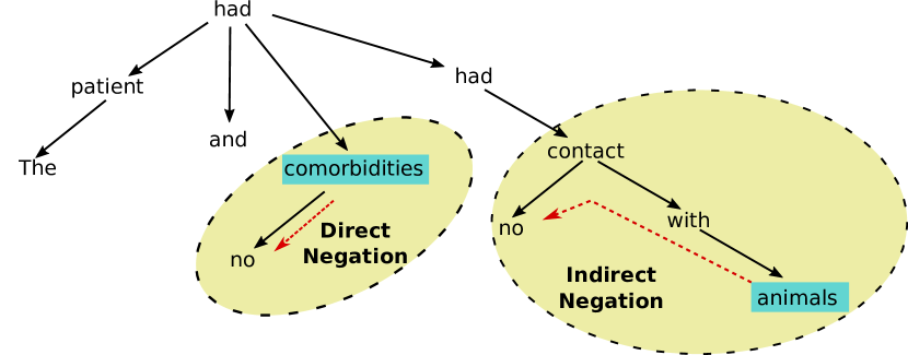
Direct Negation Detection: In this negation detection, we search for a negation cue among the neighbors of $\mathcal{I}_{t}$ in $\mathcal{D}_{\mathcal{I}_{t}}$. If a negation cue is found, then the output of $\mathcal{I}_{t}$ is classified as N.
Indirect Negation Detection. Absence of a negation cue in the neighborhood of $\mathcal{I}_{t}$ drives us to perform indirect negation detection. In this detection, we locate those terms in $\mathcal{D}_{\mathcal{I}_{t}}$ for which $\mathcal{D}_{\mathcal{I}_{t}}$ has a directed path from each of these terms as source to $\mathcal{I}_{t}$ as target. We refer to these terms as the predecessors of $\mathcal{I}_{t}$ in $\mathcal{D}_{\mathcal{I}_{t}}$. Then, we search for negation cues in the neighborhood of each predecessor. If we find a negation cue around a predecessor, we assume that the indicator $\mathcal{I}_{t}$ is also affected by this negation and we classify the output of $\mathcal{I}_{t}$ as N. For example, consider the sentence $\mathcal{S}_{6}=$The patient had no comorbidities and had no contact with animals. and the directed dependency graph corresponding to $\mathcal{S}_{6}$ is shown in Figure 4. Sentence $\mathcal{S}_{6}$ contains the seed indicators comorbidities for comorbidities and animals for animal contact. In Figure 4, we observe direct negation detection for comorbidities as the negation cue no is located in the neighborhood of the indicator comorbidities. However, for animal contact, we observe indirect negation detection as the negation cue no is situated in the neighborhood of the term contact which is one of the predecessors of the indicator animals.

Figure 4: Directed dependency graph corresponding to $\mathcal{S}_{6}$ showing direct and indirect negation detection

Therefore, for a clinical feature we have $K+1$ indicators and the classification output Y or N from each indicator. The final output for a feature is obtained via majority voting on the outputs of the indicators.

Input : seed indicator, word embeddings for each term in $\mathcal{W}$, negation cues, $\mathcal{SC}_{n}$

Output : Y or N

1 Growth of seed indicator using word embeddings to generate $K+1$ indicators represented as $\mathcal{I}_{t}\forall t\in 1,2,\ldots,K+1$;

2 for each $\mathcal{I}_{t}$ do

3       Iterate over each sentence in $\mathcal{SC}_{n}$ and identify the first sentence $\mathcal{S}_{{I}_{t}}$ mentioning ${I}_{t}$;

4       Construct the directed dependency graph $\mathcal{D}_{{I}_{t}}$ (see Figure 4) for $\mathcal{S}_{{I}_{t}}$;

5       $N_{{I}_{t}}=$ set of terms connected to $\mathcal{I}_{t}$ in $\mathcal{D}_{{I}_{t}}$, i.e. neighbors of $\mathcal{I}_{t}$;

6       $P_{{I}_{t}}=$ predecessors of $\mathcal{I}_{t}$ in $\mathcal{D}_{{I}_{t}}$;

7       Isnegation $\leftarrow 0$;

8       if $N_{{I}_{t}}$ has a negation cue then

9             output of $\mathcal{I}_{t}$= N;

10             Isnegation $\leftarrow 1$;

11             break;

12      else

13             Iterate over each term in $P_{{I}_{t}}$ and seach for a negation cue in the neighborhood;

14             if negation cue found in neighborhood of a predecessor then

15                   output of $\mathcal{I}_{t}$= N;

16                   Isnegation $\leftarrow 1$;

17                   break;

18                  

19            

20      if $\neg$Isnegation then

21             output of $\mathcal{I}_{t}$= Y;

22            

23      

24final output = majority voting on the outputs of each $\mathcal{I}_{t}$;

Algorithm 3 Level 2 modeling

4 Experimental Evaluation

In this section, we first provide a brief description of our experimental setup, including the models for automatic extraction of line lists, human annotated line lists, accuracy metric and parameter settings.

4.1 WHO corpus

The WHO corpus used in the template learning process (see Figure 2) was downloaded from http://www.who.int/csr/don/archive/disease/en/. The corpus contains outbreak news articles related to a wide range of diseases reported during the time period 1996 to 2016. The textual content of each article was pre-processed by sentence splitting, tokenization and lemmatization using spaCy [16]. After pre-processing, the WHO corpus was found to contain 35,485 sentences resulting in a vocabulary $\mathcal{W}$ of 4447 words.

4.2 Models

We evaluated the following automated line listing models.

$\>\bullet$ Guided Deep List (SGNS): Variant of Guided Deep List with SGNS used as the word2vec model in the WHO template learning process.
$\>\bullet$ Guided Deep List (SGHS): Variant of Guided Deep List with SGHS used as the word2vec model in the WHO template learning process.
Guidedlist: Baseline model which does not use any word embedding model (absence of WHO template learning) to expand the seed indicator in order to generate $K+1$ indicators for each feature. Therefore, Guidedlist uses only a single indicator (seed indicator) to extract line list features.

4.3 Human annotated line list

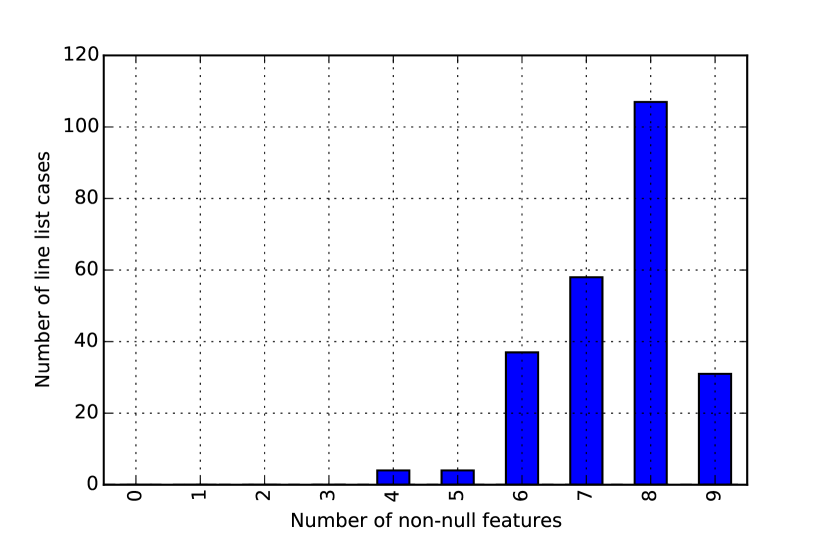
We evaluated the line list extracted by the automated line listing models against a human annotated line list for MERS outbreaks in Saudi Arabia. To create the human annotated list, patient and outcome data for confirmed MERS cases were collected from the MERS Disease Outbreak News (DONs) reports of WHO [3] and curated into a machine-readable tabular line list. In the human annotated list, total number of confirmed cases were 241 curated from 64 WHO bulletins reported during the period October 2012 to February 2015. Some of these 241 cases have missing (null) features (see Figure 1). In Figure 5, we show the distribution of non-null features in the human annotated list. We observe that majority of human annotated cases have at least 6 (out of 9) non-null features with the peak of the distribution at 8.

Figure 5: Distribution of non-null features in the human annotated line list

4.4 Accuracy metric

Matching automated line list to human annotated list.

For evaluation, the problem is: we are given a set of automated line list cases and a set of human annotated cases for a single WHO MERS bulletin. Our strategy is to costruct a bipartite graph [17] where (i) an edge exists if the automated case and the human annotated case is extracted from the same WHO bulletin and (ii) the weight on the edge denotes the quality score (QS). Quality score (QS) is defined as the number of correctly extracted features in the automated case divided by the number of non-null features in the human annotated case. We then construct a maximum weighted bipartite matching [17]. Such matchings are conducted for each WHO bulletin to extract a set of matches where each match represents a pair (automated case, human annotated case) and is also associated with a QS. Once the matches are found for all the WHO bulletins, we computed the average QS by averaging the QS values across the matches.

Once the average QS and QS for each match are computed, we also computed the accuracy for each line list feature. For the demographic and disease onset features, we computed the accuracy classification score using scikit-learn [22] by comparing the automated features against the human annotated features across the matches. The clinical features are associated with two classes - Y and N (see Figure 1). For each class, we computed the F1-score using scikit-learn [22] where F1-score can be interpreted as a harmonic mean of the precision and recall. F1-score reaches its best value at 1 and worst score at 0. Along with the F1-score for each class, we also report the average F1-score across the two classes.

4.5 Parameter settings

Each variant of Guided Deep List inherits the parameters of the word embedding models as shown in Table 5. Apart from the word embedding parameters, Guided Deep List also inherits the parameter $K$ which refers to the $K+1$ indicators for disease onset or clinical features (see Section 3). In Table 5, we provide the list of all parameters, the explored values for each parameter and the applicable models corresponding to each parameter. We selected the optimal parameter configuration for each model based on the maximum average QS value as well as maximum average of the individual feature accuracies across the matches.

5 Results

In this section we try to ascertain the efficacy and applicability of Guided Deep List by investigating some of the pertinent questions related to the problem of automated line listing.

Multiple indicators vs single indicator - which is the better method for automated line listing?

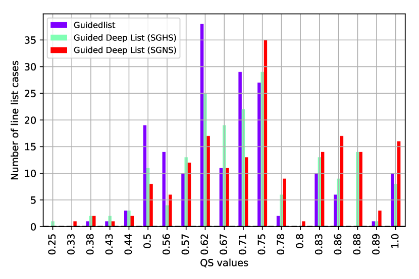
As mentioned in section 4, Guided Deep List (SGNS) and Guided Deep List (SGHS) uses multiple indicators discovered by word2vec, whereas the baseline Guidedlist uses only the seed indicator to infer line list features. We executed our automated line listing models taking as input the same set of 64 WHO MERS bulletins from which 241 human annotated line list cases were extracted. In Table 2, we observe that the number of automated line list cases (198) and the matches (182) after maximum bipartite matching is same for all the models. This is due to the reason that level 0 modeling (age and gender extraction) is the common modeling component in all the models and the number of extracted line list cases depends on the age and gender extraction (see section 3). In Table 2, we also compared the average QS achieved by each model. We observe that Guided Deep List (SGNS) is the best performing model achieving an average QS of 0.74 over Guided Deep List (SGHS) (0.71) and Guidedlist (0.67). To further validate the results in Table 2, we also show the QS distribution for each model in Figure 6 where x-axis represents the QS values and the y-axis represents the number of automated line list cases having a particular QS value. For Guidedlist, the peak of QS distribution is at 0.62. However, for Guided Deep List (SGNS) and Guided Deep List (SGHS), the peak of the distribution is at 0.75. We further observe that Guided Deep List (SGNS) extracts higher number of line list cases with a perfect QS of 1 in comparison to Guidedlist.

We also compared the models on the basis of individual accuracies of the line list features across the matches in Tables 3 and 4. In Table 3, all the models achieve similar performance for the demographic features since level 0 modeling is similar for all the models (see section 3). However, for the disease onset features, both Guided Deep List (SGNS) and Guided Deep List (SGHS) outperform the baseline achieving an average accuracy of $0.45$ and $0.43$ in comparison to Guidedlist ($0.12$) respectively. Guided Deep List (SGNS) is the best performing model for onset date. However, for hospitalization date and outcome date, Guided Deep List (SGHS) is the better performing model than Guided Deep List (SGNS). In Table 4, for the clinical features, we observe that Guided Deep List (SGNS) performs better than Guided Deep List (SGHS) and Guidedlist for comorbidities and specified HCW on the basis of average F1-score. Specifically, for specified HCW, Guided Deep List (SGNS) outperforms Guided Deep List (SGHS) and Guidedlist for the minority class Y. For animal contact, Guided Deep List (SGHS) emerges out to be the best performing model in terms of average F1-score, specifically outperforming the competing models for the minority class Y. Guidedlist only performs better for secondary contact, even though the performance for the minority class Y is almost similar to Guided Deep List (SGHS) and Guided Deep List (SGNS). Overall, we can conclude from Table 4 that Guided Deep List employing multiple indicators discovered via SGNS or SGHS shows superior performance than Guidedlist in majority of the scenarios, specifically for the minority class of each clinical feature. To further validate the results in Table 4, the confusion matrix for each model and each clinical feature can be found in https://github.com/sauravcsvt/KDD_linelisting.

Table 2: Average Quality Score (QS) achieved by each automated line listing model for MERS line list in Saudi Arabia. As can be seen, Guided Deep List (SGNS) shows best performance achieving an average QS of 0.73

Models	Human lists	Auto lists	Matches	Average QS
Guidedlist (baseline)	241	198	182	0.67
Guided Deep List (SGHS)	241	198	182	0.71
Guided Deep List (SGNS)	241	198	182	0.74

Figure 6: Distribution of QS values for each automated line listing model corresponding to MERS line list in Saudi Arabia. X-axis represents QS values and Y-axis represents the number of automated line list cases having a particular QS value

Table 3: Comparing the automated line listing models based on the accuracy score for the demographics and disease onset features. For the disease onset features, Guided Deep List (SGNS) emerges out to be the best performing model. However, for the demographic features, all the models achieve almost similar performance

Feature type	Features	Guidedlist (baseline)	Guided Deep List (SGHS)	Guided Deep List (SGNS)
Demographics	Age	0.87	0.91	0.87
	Gender	0.99	0.98	0.97
	Average	0.93	0.95	0.92
Disease onset	Onset date	0.01	0.01	0.37
	Hospitalization date	0.11	0.63	0.62
	Outcome date	0.48	0.66	0.36
	Average	0.20	0.43	0.45

Table 4: Comparing the performance of the automated line listing models for extracting clinical features corresponding to MERS line list in Saudi Arabia. We report the F1-score for class Y, class N and average F1-score across the two classes. For animal contact, Guided Deep List (SGHS) emerges out to be the best performing model. For comorbidities and specified HCW, Guided Deep List (SGNS) shows best performance. However, for secondary contact, Guidedlist achieve superior performance in comparison to Guided Deep List

Clinical Feature (Y:N)	Class	Guidedlist (baseline)	Guided Deep List (SGHS)	Guided Deep List (SGNS)
Animal contact (1:3)	Y	0.33	0.68	0.37
	N	0.87	0.91	0.88
	Average	0.60	0.79	0.63
Secondary contact (1:3)	Y	0.57	0.52	0.56
	N	0.86	0.70	0.72
	Average	0.71	0.61	0.64
Comorbidities (2:1)	Y	0.52	0.52	0.81
	N	0.56	0.54	0.61
	Average	0.54	0.53	0.71
Specified HCW (1:6)	Y	0.26	0.35	0.44
	N	0.95	0.93	0.90
	Average	0.61	0.64	0.67

What are beneficial parameter settings for automated line listing?

To identify which parameter settings are beneficial for automated line listing, we looked at the best parameter configuration (see Table 5) of Guided Deep List (SGNS) and Guided Deep List (SGHS) which achieved the accuracy values in Tables 2, 3 and 4. In Table 5, we explored the standard settings of each word2vec parameter (dimensionality of word embeddings, window size, negative samples and training iterations) in accordance with previous research [18]. Regarding dimensionality of word embeddings, Guided Deep List (SGHS) prefers $600$ dimensions, whereas Guided Deep List (SGNS) prefers $300$ dimensions. For the window size, both the models seem to benefit from smaller-sized (5) context windows. The number of negative samples is applicable only for Guided Deep List (SGNS) where it seems to prefer a single negative sample. Finally, for the training iterations, both the models benefit from more than 1 training iteration. This is expected as the WHO corpus used in the template learning process (see section 4) is a smaller-sized corpus with a vocabulary of only $\mathcal{W}=4447$ words. In such scenarios, word2vec models (SGNS or SGHS) generate improved embeddings with higher number of training iterations. Finally, both the models are also associated with the parameter $K$ which refers to the number of indicators $K+1$ used for extracting the disease onset and clinical features. As expected, the models prefer at least 5 indicators, along with the seed indicator to be used for automated line listing. Using higher number of indicators increases the chance of discovering an informative indicator for a line list feature.

Table 5: Parameter settings in Guided Deep List (SGNS) and Guided Deep List (SGHS) for which both the models achieve optimal performance in terms of average QS and individual feature accuracies corresponding to MERS line list in Saudi Arabia. Non-applicable combinations are marked by NA

Models	Dimensionality (300:600)	Window size (5:10:15)	Negative samples (1:5:15)	Training Iterations (1:2:5)	Indicators ($K$ = 3:5:7)
Guided Deep List (SGHS)	600	5	NA	5	7
Guided Deep List (SGNS)	300	5	1	2	5

Which indicator keywords discovered using word2vec contribute to the improved performance of Guided Deep List?

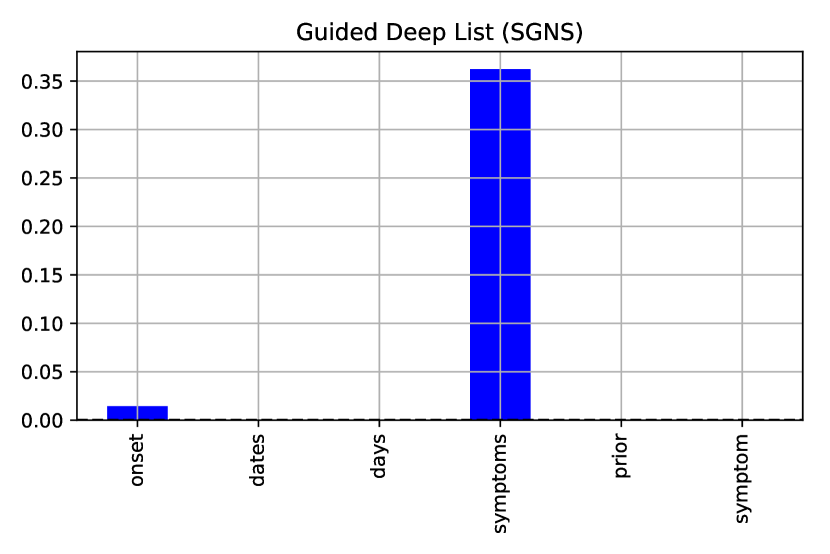
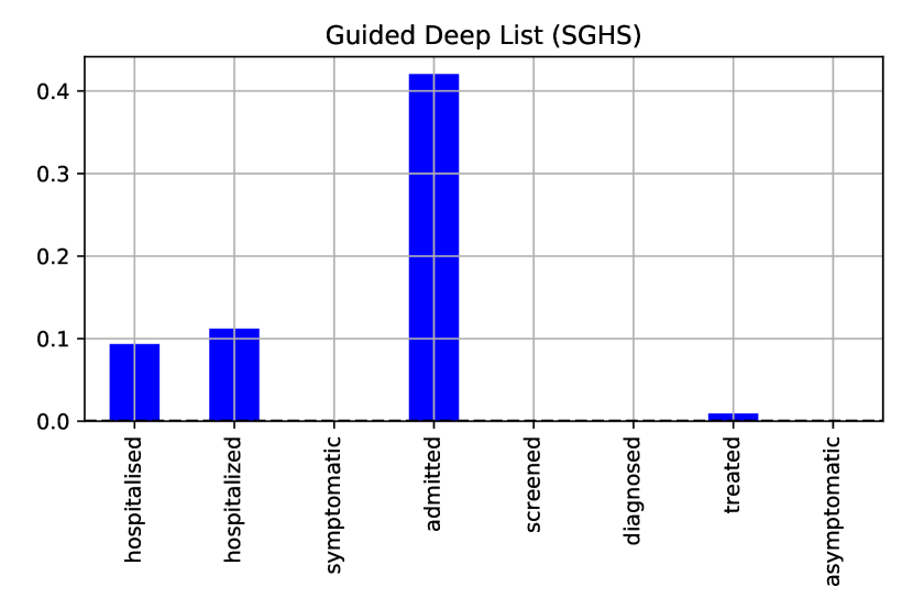
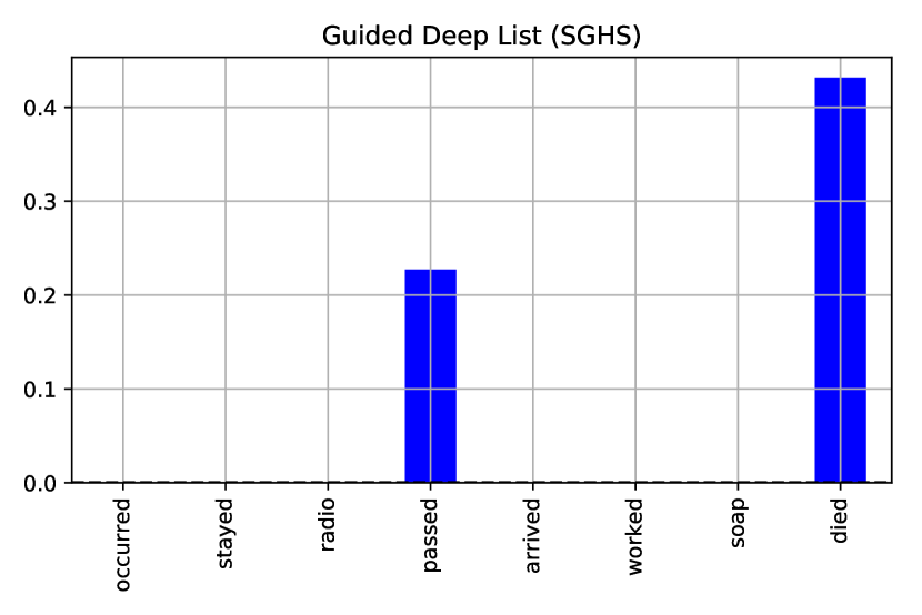
Next, we investigate the informative indicators discovered using word2vec which contribute to the improved performance of Guided Deep List (SGNS) or Guided Deep List (SGHS) in Tables 3 and 4. In Figure 7, we show the accuracies (or, average F1-score) of individual indicators (including the seed indicator) corresponding to the best performing model for a particular line list feature. Regarding onset date (see Figure 7(a)), Guided Deep List (SGNS) is the best performing model and the seed indicator provided as input is onset. We observe that symptoms is the most informative indicator achieving an accuracy of 0.36 similar to the overall accuracy (see Table 3). Rest of the indicators (including the seed indicator) achieve negligible accuracies and therefore, do not contribute to the overall performance of Guided Deep List (SGNS). Similary, for hospitalization date with the seed keyword hospitalization provided as input, admitted emerges out to be most informative indicator followed by the seed indicator, hospitalised and treated (see Figure 7(b)). Finally, for the outcome date, died (seed indicator) and passed are the two most informative indicators as observed in Figure 7(c).

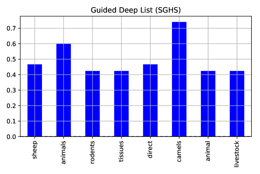
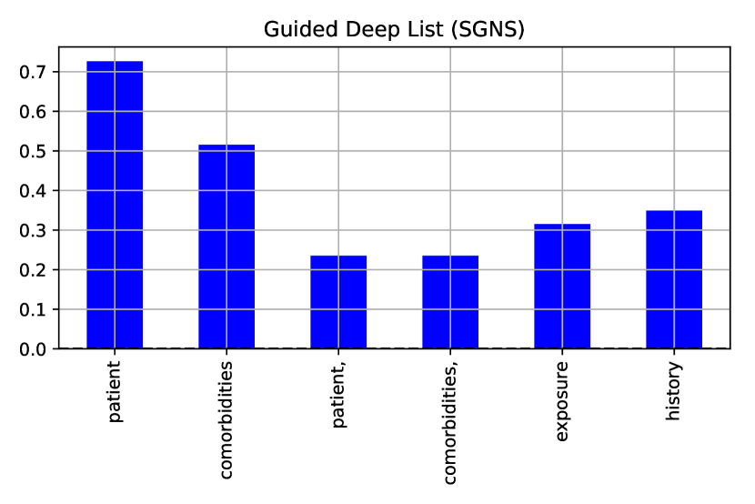
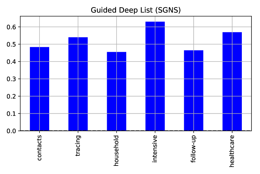
Regarding the clinical features, we show the average F1-score of individual indicators. For animal contact, the seed indicator provided as input is animals. We observe in Figure 7(d) that the most informative indicator for animal contact is camels followed by indicators such as animals (seed), sheep and direct. This shows that contact with camels is the major transmission mechanism for MERS disease. The informative indicators found for comorbidities are patient, comorbidities and history. Finally, regarding specified HCW, the informative indicators discovered are healthcare (seed), tracing and intensive.

(a) Onset date

(b) Hospital date

(c) Outcome date

(d) Animal contact

(e) Comorbidities

(f) Specified HCW

Figure 7: Accuracy of individual indicators (including the seed indicator) discovered via word2vec methods in Guided Deep List (SGNS) or Guided Deep List (SGHS) for each line list feature. For clinical features, we show the average F1-score. This figure depicts the informative indicators (indicators showing higher accuracies or F1-scores) which contribute to the improved performance of Guided Deep List (SGNS) or Guided Deep List (SGHS) for a particular feature. E.g. for animal contact, the most informative indicator contributing to the superior performance of Guided Deep List (SGHS) is camels followed by animals (seed), sheep and direct

Does indirect negation detection play an useful role in extracting clinical features?

In level 2 modeling for extracting clinical features, both direct and indirect negation detection are used. For more details, please see section 3. To identify if indirect negation detection contributes positively, we compared the performance of Guided Deep List with and without indirect negation detection for each clinical feature in Table 6 by reporting the F1-score for each class as well as average F1-score. We observe that indirect negation detection has a positive effect on the performance for animal contact and secondary contact. However, for comorbidities and specified HCW, indirect negation detection plays an insignificant role.

Table 6: Comparing the performance of Guided Deep List on extraction of clinical features with or without indirect negation for MERS line list in Saudi Arabia. It can be seen that indirect negation improves the performance of Guided Deep List for animal contact and secondary contact.

Clinical Feature	Class	Direct Negation	Direct + Indirect Negation
Animal contact	Y	0.56	0.63
	N	0.80	0.90
	Average	0.68	0.77
Secondary contact	Y	0.55	0.54
	N	0.65	0.72
	Average	0.60	0.63
Comorbidities	Y	0.86	0.82
	N	0.64	0.62
	Average	0.75	0.72
Specified HCW	Y	0.44	0.44
	N	0.90	0.90
	Average	0.67	0.67

What insights can epidemiologists gain about the MERS disease from automatically extracted line lists?

Finally, we show some of the utilities of automated line lists by inferring different epidemiological insights from the line list extracted by Guided Deep List.
Demographic distribution. In Figure 1, we show the age and gender distribution of the affected individuals in the extracted line list. We observe that males are more prone to getting infected by MERS rather than females. This is expected as males have a higher probability of getting contacted with infected animals (animal contact) or with each other (secondary contact). Also individuals aged between 40 and 70 are more prone to getting infected as evident from the age distribution.
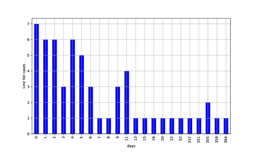
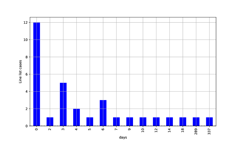
Analysis of disease onset features. We analyzed the symptoms-to-hospitalization period by analyzing the difference (in days) between onset date and hospitalization date in the extracted line list as shown in Figure 8(a). We observe that most of the affected individuals with onset of symptoms got admitted to the hospital either on the same day or within 5 days. This depicts a prompt responsiveness of the concerned health authorities in Saudi Arabia in terms of admitting the individuals showing symptoms of MERS. In Figure 8(b), we also show a distribution of the hospitalization-to-outcome period (in days). Interestingly, we see that the distribution has a peak at 0 which indicates that most of the infected individuals admitted to the hospital died on the same day indicating high fatality rate of MERS case.

(a) Symptoms-to-hospitalization period distribution

(b) Hospitalization-to-outcome period distribution

Figure 8: Analysis of disease onset features in the extracted line list

Supplementary Information

Codes and data for this manuscript are available at https://github.com/sauravcsvt/KDD_linelisting.

References

- [1] Lau, E. H. et al. Accuracy of epidemiological inferences based on publicly available information: retrospective comparative analysis of line lists of human cases infected with influenza a (h7n9) in china. BMC medicine 12, 88 (2014).
- [2] Majumder, M. S., Rivers, C., Lofgren, E. & Fisman, D. Estimation of mers-coronavirus reproductive number and case fatality rate for the spring 2014 saudi arabia outbreak: insights from publicly available data. PLOS Currents Outbreaks (2014).
- [3] WHO. Coronavirus infections: Disease outbreak news (2016). URL http://www.who.int/csr/don/archive/disease/coronavirus_infections/en/.
- [4] Mikolov, T., Chen, K., Corrado, G. & Dean, J. Efficient estimation of word representations in vector space. CoRR abs/1301.3781 (2013). URL http://arxiv.org/abs/1301.3781.
- [5] Mikolov, T., Sutskever, I., Chen, K., Corrado, G. S. & Dean, J. Distributed representations of words and phrases and their compositionality. In 26th Annual Conference on Neural Information Processing Systems, 3111–3119 (2013).
- [6] Le, Q. V. & Mikolov, T. Distributed representations of sentences and documents. In ICML, vol. 14, 1188–1196 (2014).
- [7] Mikolov, T., Yih, W. & Zweig, G. Linguistic regularities in continuous space word representations. In Human Language Technologies: Conference of the NAACL, 746–751 (2013). URL http://aclweb.org/anthology/N/N13/N13-1090.pdf.
- [8] Levy, O. & Goldberg, Y. Linguistic regularities in sparse and explicit word representations. In Proceedings of the Eighteenth Conference on CoNLL, 171–180 (2014). URL http://aclweb.org/anthology/W/W14/W14-1618.pdf.
- [9] Wu, F. & Weld, D. S. Open information extraction using wikipedia. In Proceedings of the 48th Annual Meeting of the Association for Computational Linguistics, 118–127 (Association for Computational Linguistics, 2010).
- [10] Ou, Y. & Patrick, J. Automatic negation detection in narrative pathology reports. Artificial intelligence in medicine 64, 41–50 (2015).
- [11] Sohn, S., Wu, S. & Chute, C. G. Dependency parser-based negation detection in clinical narratives. AMIA Summits on Translational Science proceedings AMIA Summit on Translational Science 2012, 1–8 (2012).
- [12] Ballesteros, M. et al. Ucm-2: a rule-based approach to infer the scope of negation via dependency parsing. In Proceedings of the First Joint Conference on Lexical and Computational Semantics-Volume 1: Proceedings of the main conference and the shared task, and Volume 2: Proceedings of the Sixth International Workshop on Semantic Evaluation, 288–293 (Association for Computational Linguistics, 2012).
- [13] Bunescu, R. C. & Mooney, R. J. A shortest path dependency kernel for relation extraction. In Proceedings of the conference on human language technology and empirical methods in natural language processing, 724–731 (Association for Computational Linguistics, 2005).
- [14] Levy, O. & Goldberg, Y. Dependency-based word embeddings. In ACL (2), 302–308 (2014).
- [15] Muthiah, S. et al. Planned protest modeling in news and social media. In AAAI, 3920–3927 (2015).
- [16] Honnibal, M. & Johnson, M. An improved non-monotonic transition system for dependency parsing. In Proceedings of the 2015 Conference on Empirical Methods in Natural Language Processing, 1373–1378 (Association for Computational Linguistics, Lisbon, Portugal, 2015). URL https://aclweb.org/anthology/D/D15/D15-1162.
- [17] Ramakrishnan, N. et al. ‘Beating the news’ with EMBERS: Forecasting civil unrest using open source indicators. In Proceedings of the 20th ACM SIGKDD International Conference on Knowledge Discovery and Data Mining, 1799–1808 (ACM, 2014).
- [18] Levy, O., Goldberg, Y. & Dagan, I. Improving distributional similarity with lessons learned from word embeddings. TACL 3, 211–225 (2015). URL https://tacl2013.cs.columbia.edu/ojs/index.php/tacl/article/view/570.
- [19] Levy, O. & Goldberg, Y. Dependency-based word embeddings. In Proceedings of the 52nd Annual Meeting of the ACL, 302–308 (2014). URL http://aclweb.org/anthology/P/P14/P14-2050.pdf.
- [20] Ghosh, S., Chakraborty, P., Cohn, E., Brownstein, J. S. & Ramakrishnan, N. Characterizing diseases from unstructured text: A vocabulary driven word2vec approach. In Proceedings of the 25th ACM International on Conference on Information and Knowledge Management, 1129–1138 (ACM, 2016).
- [21] Diaz, A., Ballesteros, M., Carrillo-de Albornoz, J. & Plaza, L. Ucm at trec-2012: Does negation influence the retrieval of medical reports? Tech. Rep., DTIC Document (2012).
- [22] Pedregosa, F. et al. Scikit-learn: Machine learning in Python. Journal of Machine Learning Research 12, 2825–2830 (2011).