Two- and Three-Dimensional Probes of Parity in Primordial Gravity Waves

Abstract

We show that three-dimensional information is critical to discerning the effects of parity violation in the primordial gravity-wave background. If present, helical gravity waves induce parity-violating correlations in the cosmic microwave background (CMB) between parity-odd polarization $B$-modes and parity-even temperature anisotropies ($T$) or polarization $E$-modes. Unfortunately, $EB$ correlations are much weaker than would be naively expected, which we show is due to an approximate symmetry resulting from the two-dimensional nature of the CMB. The detectability of parity-violating correlations is exacerbated by the fact that the handedness of individual modes cannot be discerned in the two-dimensional CMB, leading to a noise contribution from scalar matter perturbations. In contrast, the tidal imprints of primordial gravity waves fossilized into the large-scale structure of the Universe are a three-dimensional probe of parity violation. Using such fossils the handedness of gravity waves may be determined on a mode-by-mode basis, permitting future surveys to probe helicity at the percent level if the amplitude of primordial gravity waves is near current observational upper limits.

Nature is parity violating: the electroweak $W$ bosons couple only to left-handed particles and right-handed antiparticles, violating both parity ($P$) and charge conjugation ($C$) maximally. Thus, weak nuclear processes produce only left-handed neutrinos and right-handed antineutrinos. In this context, it is natural to ask whether gravitational processes violate parity, in particular, whether such violations may be present in the cosmological gravity-wave background. If detected, the stochastic background of long wavelength gravity waves would provide a uniquely powerful probe of the very early Universe. A variety of sources of gravitational parity violation have been considered, from fundamental quantum gravity effects to rolling inflationary axions (Lue et al., 1999; Contaldi et al., 2008; Takahashi and Soda, 2009; Sorbo, 2011). Each of these could have have left an imprint on the net helicity of the gravity wave background, namely the preferred excitation of one circular polarization over the other.

An additional reason to be interested in a helical primordial gravity-wave background is that it would have brought nonperturbative standard model processes into play, potentially explaining the cosmological matter–antimatter asymmetry Alexander et al. (2006). Because of the chiral nature of neutrinos, lepton number conservation is violated in the standard model by a gravitational anomaly: $\partial_{\mu}J^{\mu}_{L}=(3/32\pi^{2})\varepsilon^{\alpha\beta\gamma\sigma}R_{\alpha\beta}^{\quad\rho\sigma}R_{\rho\sigma\gamma\sigma}$, where $J^{\mu}_{L}$ is the lepton current and $R_{\alpha\beta\rho\sigma}$ is the Riemann curvature tensor Alvarez-Gaume and Witten (1984). Any process that generates a parity-violating ensemble of gravity waves will necessarily give the anomaly a nonzero expectation value, driving a lepton asymmetry number that would, at high temperature, be converted into a baryon asymmetry by electroweak “sphaleron” processes.

The net helicity of the gravity-wave background is thus of fundamental interest and importance. In this Letter, we consider its detectability, and the role played by the dimensionality of potential probes. Gravitational waves induce both CMB temperature and polarization anisotropies Seljak and Zaldarriaga (1997); Kamionkowski et al. (1997). While temperature and $E$-mode polarization patterns are also induced by scalar perturbations, at linear order $B$-mode polarization is only produced by gravity waves. Cross-correlations between the parity-odd $B$-mode polarization and either the parity-even $E$-mode polarization or temperature perturbations are parity violating. These correlations vanish if the gravity wave background has no net helicity, as is the case in standard inflationary scenerios.

Saito et al. (2007) calculated the resulting $EB$ and $TB$ correlations for a primordial gravity-wave background with net helicity. They found that even in the maximally helical case—with all gravity waves having the same circular polarization—$EB$ correlations are highly suppressed, with cross-correlation coefficients of order $\sim 10^{-2}$. The $TB$ correlations are larger, with correlation coefficients closer to unity, but these are difficult to detect against the large background of noise arising from the scalar matter perturbations. Detecting helicity in the CMB is thus very difficult: even for a cosmic-variance limited measurement of the CMB polarization, parity violation is never detectable at $>3\sigma$ if the amplitude of primordial gravity waves—parameterized by the tensor-to-scalar ratio $r$—is less than $0.02$ (Gluscevic and Kamionkowski, 2010). Even at the current upper limit of $r<0.07$ (BICEP2 Collaboration et al., 2016), only fractional helicity power above $\Delta\chi=50\%$ could be detected. Indeed a recent search for such correlations concluded that there is little hope for their detection in current or upcoming CMB surveys (Gerbino et al., 2016).

After introducing some formalism for gravity wave helicity, we show that the suppression of the $EB$ correlations is a direct result of the two-dimensional nature of the CMB. We then consider whether helicity can be detected using the three-dimensional tidal imprints of gravity waves fossilized into the large-scale structure, as introduced by Masui and Pen (2010). We show that the limitations of the CMB are removed in three dimensions, in principle permitting future surveys to detect even weak helicity.

Helical gravity waves.—Gravity waves (which we will also refer to as tensor modes) are encoded in the transverse, traceless part of the linearized metric perturbations $h_{ab}(\bm{\mathrm{x}})$, which has two degrees of freedom. In Fourier space, $h_{ab}(\bm{\mathrm{K}})=\int d^{3}\bm{\mathrm{x}}e^{-i\bm{\mathrm{K}}\cdot\bm{\mathrm{x}}}h_{ab}(\bm{\mathrm{x}})$, these two degrees of freedom can be described by the circular polarization amplitudes $h_{R}$ and $h_{L}$ as

$$h_{ab}(\bm{\mathrm{K}}) =h_{R}(\bm{\mathrm{K}})e^{R}_{ab}(\bm{\hat{\mathrm{K}}})+h_{L}(\bm{\mathrm{K}})e^{L}_{ab}(\bm{\hat{\mathrm{K}}})$$

$$e^{R}_{ab}(\bm{\hat{\mathrm{K}}}) \equiv\frac{1}{\sqrt{2}}\left[e^{+}_{ab}(\bm{\hat{\mathrm{K}}})+ie^{\times}_{ab}(\bm{\hat{\mathrm{K}}})\right]$$

$$e^{L}_{ab}(\bm{\hat{\mathrm{K}}}) \equiv\frac{1}{\sqrt{2}}\left[e^{+}_{ab}(\bm{\hat{\mathrm{K}}})-ie^{\times}_{ab}(\bm{\hat{\mathrm{K}}})\right],$$ (1)

where $e^{+}_{ab}(\bm{\hat{\mathrm{K}}})\equiv\hat{e}^{\theta_{K}}_{a}\hat{e}^{\theta_{K}}_{b}-\hat{e}^{\phi_{K}}_{a}\hat{e}^{\phi_{K}}_{b}$ and $e^{\times}_{ab}(\bm{\hat{\mathrm{K}}})\equiv\hat{e}^{\theta_{K}}_{a}\hat{e}^{\phi_{K}}_{b}+\hat{e}^{\phi_{K}}_{a}\hat{e}^{\theta_{K}}_{b}$, and $\bm{\hat{\mathrm{e}}}^{\theta_{K}}$ and $\bm{\hat{\mathrm{e}}}^{\phi_{K}}$ are the spherical polar unit vectors relative to $\bm{\mathrm{K}}$. This definition is consistent with the International Astronomical Union’s definition of circular polarization for electromagnetic radiation, where a right-hand circular wave’s instantaneous spatial configuration forms a left-handed screw (Hamaker and Bregman, 1996).

Translational invariance of the statistical ensemble dictates that the only nonzero correlators have zero net momentum: for this reason only $h_{ab}(\bm{\mathrm{K}})$ and $h_{ab}(-\bm{\mathrm{K}})=h_{ab}(\bm{\mathrm{K}})^{*}$ can be correlated in a statistically homogeneous ensemble. The left- and right-handed circular modes have opposite helicity, meaning that they transform as $e^{\pm 2i\alpha}$ under rotations by $\alpha$ about $\bm{\mathrm{K}}$. It follows that the only rotational invariant (helicity zero) combinations of $h_{ab}(\bm{\mathrm{K}})$ and $h_{ab}(-\bm{\mathrm{K}})$ are $LL$ or $RR$ (in obvious notation). These correlators are perfectly consistent with homogeneity and isotropy, although they individually violate parity. Any $RL$ correlation is prohibited by the combination of statistical homogeneity and isotropy.

The surviving correlations can be written in terms of power spectra:

$$\langle h_{ab}(\bm{\mathrm{K}})h_{cd}(\bm{\mathrm{K}}^{\prime})\rangle=(2\pi)^{3}\delta^{3}(\bm{\mathrm{K}}+\bm{\mathrm{K}}^{\prime})$$

$$\phantom{=}\times\left[e^{R}_{ab}(\bm{\hat{\mathrm{K}}})e^{R}_{cd}(-\bm{\hat{\mathrm{K}}})P_{R}(K)+e^{L}_{ab}(\bm{\hat{\mathrm{K}}})e^{L}_{cd}(-\bm{\hat{\mathrm{K}}})P_{L}(K)\right],$$ (2)

where $\delta^{3}(\bm{\mathrm{K}})$ is the three-dimensional Dirac delta function. This can be rewritten

$$\langle h_{ab}(\bm{\mathrm{K}})h_{cd}(\bm{\mathrm{K}}^{\prime})\rangle=(2\pi)^{3}\delta^{3}(\bm{\mathrm{K}}+\bm{\mathrm{K}}^{\prime})\frac{P_{h}(K)}{4}$$

$$\phantom{=}\times\left\{\left[e^{R}_{ab}(\bm{\hat{\mathrm{K}}})e^{R}_{cd}(-\bm{\hat{\mathrm{K}}})+e^{L}_{ab}(\bm{\hat{\mathrm{K}}})e^{L}_{cd}(-\bm{\hat{\mathrm{K}}})\right]\right.$$

$$\phantom{=}\left.+\Delta\chi(K)\left[e^{R}_{ab}(\bm{\hat{\mathrm{K}}})e^{R}_{cd}(-\bm{\hat{\mathrm{K}}})-e^{L}_{ab}(\bm{\hat{\mathrm{K}}})e^{L}_{cd}(-\bm{\hat{\mathrm{K}}})\right]\right\},$$ (3)

where we have defined the tensor power spectrum $P_{h}\equiv 2(P_{R}+P_{L})$ and the fractional helicity spectrum $\Delta\chi\equiv 2(P_{R}-P_{L})/P_{h}$, with $|\Delta\chi|=1$ corresponding to maximal helicity. The factor of $2$ is present by convention (Komatsu et al., 2009).

The tensor expressions in square brackets lie in the plane perpendicular to $\bm{\mathrm{K}}$ and are rotationally invariant within this plane, as required by statistical isotropy. It is always possible to rewrite a rotationally invariant tensor in terms of the two-dimensional Kronecker delta, $\delta_{ab}-\hat{K}_{a}\hat{K}_{b}$ and the two-dimensional Levi-Civita symbol, $\hat{K}^{c}\varepsilon_{cab}$. Inserting the definitions of the polarization tensors, the above expression can be reduced to

$$\langle h_{ab}(\bm{\mathrm{K}})h_{cd}(\bm{\mathrm{K}}^{\prime})\rangle =(2\pi)^{3}\delta^{3}(\bm{\mathrm{K}}+\bm{\mathrm{K}}^{\prime})\frac{P_{h}(K)}{4}\left[w_{abcd}(\bm{\hat{\mathrm{K}}})+\Delta\chi(K)v_{abcd}(\bm{\hat{\mathrm{K}}})\right]$$

$$w_{abcd}(\bm{\hat{\mathrm{K}}}) \equiv(\delta_{ad}-\hat{K}_{a}\hat{K}_{d})(\delta_{bc}-\hat{K}_{b}\hat{K}_{c})+(\delta_{ac}-\hat{K}_{a}\hat{K}_{c})(\delta_{bd}-\hat{K}_{b}\hat{K}_{d})-(\delta_{ab}-\hat{K}_{a}\hat{K}_{b})(\delta_{cd}-\hat{K}_{c}\hat{K}_{d})$$

$$v_{abcd}(\bm{\hat{\mathrm{K}}}) \equiv-i\left[(\delta_{ac}-\hat{K}_{a}\hat{K}_{c})\hat{K}_{e}\varepsilon^{e}_{\phantom{a}bd}+\hat{K}_{f}\varepsilon^{f}_{\phantom{a}ac}(\delta_{bd}-\hat{K}_{b}\hat{K}_{d})\right].$$ (4)

The two power spectra $P_{h}(K)$ and $\Delta\chi(K)$ can be isolated through contractions of these two point functions (Waelkens et al., 2009):

$$\langle h^{ab}(\bm{\mathrm{K}})h_{ab}(\bm{\mathrm{K}}^{\prime})\rangle=(2\pi)^{3}\delta^{3}(\bm{\mathrm{K}}+\bm{\mathrm{K}}^{\prime})P_{h}(K)$$

$$\langle h^{ab}(\bm{\mathrm{K}})(-i\hat{K}^{d}\varepsilon_{da}^{\phantom{a}\phantom{a}c})h_{cb}(\bm{\mathrm{K}}^{\prime})\rangle$$

$$\qquad\qquad=(2\pi)^{3}\delta^{3}(\bm{\mathrm{K}}+\bm{\mathrm{K}}^{\prime})\Delta\chi(K)P_{h}(K).$$ (5)

Here $-i\hat{K}^{c}\varepsilon_{ca}^{\phantom{a}\phantom{a}b}$ acts as the gravity wave helicity operator, noting that (Saito et al., 2007)

$$-i\hat{K}^{c}\varepsilon_{ca}^{\phantom{a}\phantom{a}d}e^{R}_{db}=e^{R}_{ab},\qquad-i\hat{K}^{c}\varepsilon_{ca}^{\phantom{a}\phantom{a}d}e^{L}_{db}=-e^{L}_{ab}.$$ (6)

Figure 1 shows a visualization of a Gaussian random gravity-wave field with and without helicity. The qualitative difference between a helical and nonhelical field when observed in three dimensions is obvious, while on any planar slice perpendicular to $\bm{\hat{\mathrm{K}}}$ the fields are statistically indistinguishable. For nonperpendicular slicings the fields are distinguishable since the slicing will cut through phase fronts, but become indistinguishable once all orientations of $\bm{\hat{\mathrm{K}}}$ are superimposed. This is in essence why detecting helicity with a two dimensional probe is difficult, as we now show explicitly for the CMB.

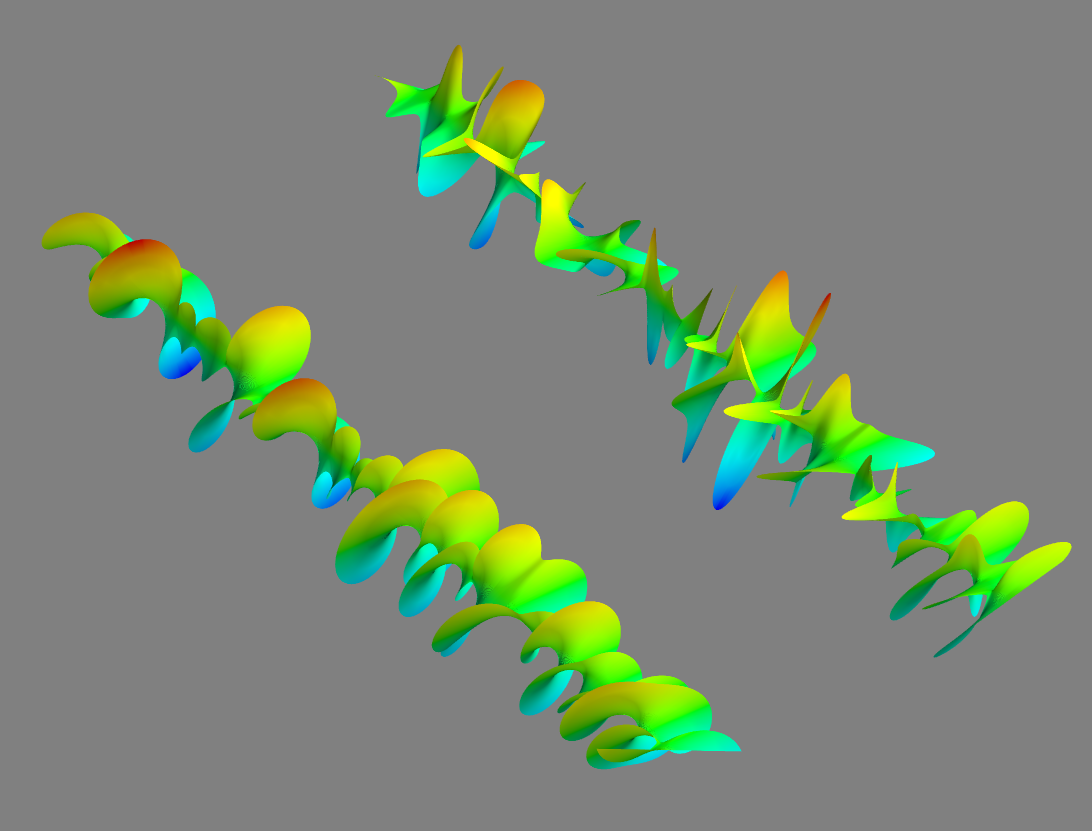
Figure 1: Visualization of gravity-wave helicity. Shown is the instantaneous strain for two pseudo-1D tensor fields with strain in the $x-y$ plane and wave numbers aligned with the $z$ axis. The width and orientation of the ribbons correspond to magnitude and orientation of the strain. The two fields are generated from the same realization of random numbers but the lower field has all power in the right-hand circular polarization ($\Delta\chi=1$), whereas the power in the upper field is distributed equally between left- and right-hand circular polarizations ($\Delta\chi=0$). The realization is drawn from a band-limited white power spectrum.

Cosmic microwave background.—If primordial gravity waves had net helicity, one might naively expect the $EB$ angular power spectrum to be $C_{\ell}^{EB}\sim\Delta\chi(C_{\ell}^{BB}C_{\ell}^{(T),EE})^{1/2}$, where the superscript $(T)$ indicates that only the contribution from tensor perturbations is included. Indeed $C_{\ell}^{TB}\sim\Delta\chi(C_{\ell}^{BB}C_{\ell}^{(T),TT})^{1/2}$ roughly holds. Instead Saito et al. (2007) showed that $C_{\ell}^{EB}$ is two orders of magnitude smaller than this expectation, making these correlations undetectable. The $TB$ correlations are hard to detect since the temperature anisotropies get a large contribution from scalar matter perturbations (especially above $\ell\sim 50$) and the error on the correlations is $\Delta C_{\ell}^{TB}\propto(C_{\ell}^{TT}C_{\ell}^{BB})^{1/2}$, i.e. including the contribution from scalar perturbations. That scalar perturbations induce noise in this correlation is itself a consequence of the loss of geometric information in the 2D projection.

We now show that the suppression of $C_{\ell}^{EB}$ is due to the two-dimensional nature of the CMB. CMB polarization is generated by the gravity-wave strain projected onto the two-dimensional surface of last scattering (Hu and White, 1997). This strain generates a local quadrupole moment in the photon distribution seen by electrons at last scatter, which perturbs the observed CMB radiation through Thompson scattering. The strain in the line-of-sight direction has no effect on the polarization, since the cross-section for colinear and antilinear scattering vanishes. Like polarization, the projected strain is a two-dimensional, rank-2 tensor, which can be decomposed into a convergence, $E$-mode shear and $B$-mode shear. These induce temperature anisotropies, $E$-mode polarization, and $B$-mode polarization respectively.

In the absence of parity symmetry, the approximate reflective symmetry about the surface of last scattering forces the $EB$ correlations to nearly vanish. For an approximately flat-sky patch of the CMB, an observer on the other side of the last scattering surface would see an identical projected strain (and thus CMB polarization) as we would, except reflected. The reflection causes a sign flip to only the observed $B$-modes and thus that observer would measure the opposite $EB$ correlations as we do. Since that observer lives in the same Universe that we do, they expect the same power spectra and thus the $EB$ power spectrum must vanish for a flat sky. This is true independent of the source of the polarization-generating photon quadrupole, and applies for helical tensor and vector modes.

To show this formally, we derive the $EB$ power spectrum within the flat-sky approximation. The detailed derivation is given in the Supplementary Material and here we present an abbreviated version. We write the contribution to the projected strain from a single mode with wave vector $\bm{\mathrm{K}}$ as

$$\mathcal{H}^{\perp}_{ab}(\bm{\hat{\mathrm{n}}},\bm{\mathrm{K}},\chi) \equiv\left[\delta^{\perp}_{ac}\delta^{\perp}_{bd}-\frac{1}{2}\delta^{\perp}_{ab}\delta^{\perp}_{cd}\right]e^{i\chi\bm{\hat{\mathrm{n}}}\cdot\bm{\mathrm{K}}}h^{cd}(\bm{\mathrm{K}}).$$ (7)

Here $\delta^{\perp}_{ab}\equiv\delta_{ab}-\hat{n}_{a}\hat{n}_{b}$ and $\chi$ is the comoving radial distance. The expression in square brackets serves to project the strain into the plane perpendicular to the line of sight (since the line-of-sight component does not induce polarization), and removes the trace to isolate the quadrupole. The polarization induced by this strain is (Kamionkowski and Kovetz, 2016)

$$\mathcal{P}_{ab}(\bm{\hat{\mathrm{n}}}) =2\int_{0}^{\chi_{i}}d\chi\int\frac{d^{3}\bm{\mathrm{K}}}{(2\pi)^{3}}S^{(T)}_{P}(K,\chi)\mathcal{H}^{\perp}_{ab}(\bm{\hat{\mathrm{n}}},\chi,\bm{\mathrm{K}}).$$ (8)

Here, $S^{(T)}_{P}(K,\chi)$ is the polarization source function for tensors, whose definition is given in Seljak and Zaldarriaga (1996). It includes all the Boltzmann physics of how gravity waves induce CMB polarization. Note that it includes the transfer function of the gravity waves and $h_{ab}$ is understood to represent the primordial value. Crucially, $S^{(T)}_{P}$ depends only on the magnitude of the wave vector, $K$, and on our time coordinate $\chi$, i.e. on the evolution of the tensor mode and photons. The geometrical dependence of the polarization (dependence on $\bm{\hat{\mathrm{n}}}$ and $\bm{\hat{\mathrm{K}}}$) is encoded in $\mathcal{H}^{\perp}_{ab}$.

On a flat patch of sky centred on the $\bm{\hat{\mathrm{n}}}=\bm{\hat{\mathrm{z}}}$ direction, Equation 8 can be Fourier transformed to be a function of $\bm{\mathrm{\ell}}$, the variable Fourier conjugate to $\bm{\hat{\mathrm{n}}}$. The Fourier transform picks out only modes with $\delta^{\perp}_{ab}K^{b}=\ell_{a}/\chi$ as contributing to each $\bm{\mathrm{\ell}}$, and we define $\bm{\mathrm{K}}_{\ell}\equiv\bm{\mathrm{\ell}}/\bar{\chi}+\bm{\hat{\mathrm{z}}}K_{\parallel}$. In this space the $E$- and $B$-mode polarization tensors have simple forms:

$$e^{\perp E}_{ab}(\bm{\hat{\mathrm{\ell}}}) =\sqrt{2}\left(\hat{\ell}_{a}\hat{\ell}_{b}-\frac{1}{2}\delta^{\perp}_{ab}\right)$$

$$e^{\perp B}_{ab}(\bm{\hat{\mathrm{\ell}}}) =\frac{\sqrt{2}}{2}\left(\hat{\ell}_{a}\hat{e}^{\phi_{\ell}}_{b}+\hat{e}^{\phi_{\ell}}_{a}\hat{\ell}_{b}\right),$$ (9)

Decomposing $\mathcal{P}_{ab}(\bm{\mathrm{\ell}})$ into $E$ and $B$ modes as $\mathcal{P}_{ab}=e^{\perp E}_{ab}a_{E}+e^{\perp B}_{ab}a_{B}$, and noting that the projections of the gravity-wave polarization tensors onto the $E$- and $B$-mode polarization tensors can be written solely in terms of $\mu_{K_{\ell}}\equiv K_{\parallel}/K_{\ell}$, we find

$$C^{EB}(\ell) =\int_{0}^{\chi_{i}}\frac{d\chi d\chi^{\prime}}{\bar{\chi}^{2}}\int_{-\infty}^{\infty}\frac{dK_{\parallel}}{2\pi}S^{(T)}_{P}(K,\chi)S^{(T)}_{P}(K,\chi^{\prime})$$

$$~{}~{}~{}\times\sin{[(\chi-\chi^{\prime})K_{\parallel}]}(1+\mu_{K_{\ell}}^{2})\mu_{K_{\ell}}\Delta\chi(K_{\ell})P_{h}(K_{\ell}).$$ (10)

It is seen that for thin last scatter—that is if the source function $S^{(T)}_{P}$ approximates a delta function at recombination, $\chi=\chi_{*}$, which was assumed in our earlier argument—then the sine factor is zero and the correlations vanish. However, even if this is not the case (i.e if the effects of reionization are included), the integrand is antisymmetric under exchange of $\chi$ and $\chi^{\prime}$, while the integration limits are symmetric, and the correlations still vanish.

To compute $C^{TB}(\ell)$, one replaces the factor of $1+\mu_{K_{\ell}}^{2}$ with $-1+\mu_{K_{\ell}}^{2}$ in Equation Two- and Three-Dimensional Probes of Parity in Primordial Gravity Waves. One also replaces one factor of $S^{(T)}_{P}$ with $S^{(T)}_{T}$, which has an extra contribution proportional to the time derivative of the tensor transfer function $\mathcal{T}(K,\chi)$. This is because gravity wave strain induces temperature anisotropies both through Thompson scattering and through direct redshifting of CMB photons. This breaks the $\chi$, $\chi^{\prime}$ antisymmetry yielding nonvanishing correlations between $B$-modes induced by Thompson scattering and temperature modes induced by direct redshifting.

We note that this derivation applies equally well for vector modes, replacing $S^{(T)}_{P}$ and $S^{(T)}_{T}$ with the appropriate source functions: $S^{(V)}_{P}$ and $S^{(V)}_{T}$. In this case we expect the $TB$ correlations to be highly suppressed by the sine factor for mechanisms where the generation of anisotropies is confined to the last-scattering surface.

That the $EB$ correlations vanish in flat sky would seem to conflict with the full-sky calculation that finds not only nonvanishing $EB$ correlations (at the $0.01\times\Delta\chi$ level) but no $1/\ell$ suppression of $EB$ compared to $BB$ and $EE$ from tensors. We find that this is a direct result of sky curvature. In the Supplementary Material we convert the full-sky $EB$ power spectrum directly to the flat-sky expression above. This conversion includes the regular flat-sky transformation

$$\frac{2}{\pi}\int_{0}^{\infty}K^{2}dKF(K,\chi,\chi^{\prime})j_{\ell}(K\chi)j_{\ell}(K\chi^{\prime})$$

$$\qquad\qquad\rightarrow\int_{-\infty}^{\infty}\frac{dK_{\parallel}}{2\pi}F(K_{\ell},\chi,\chi^{\prime})e^{iK_{\parallel}(\chi-\chi^{\prime})},$$

where $F$ may include differential operators with respect to $\chi$ and $\chi^{\prime}$. This conversion makes approximations that are invalid before the first few oscillations of the Bessel functions, at $K\chi\sim\ell+1/2$—the contribution to the integral from the nonplanar nature of the sky. While this part of the integral is normally sub-dominant, the induced error is unsuppressed by $1/\ell$. For the $EB$ correlations, the rest of the integral vanishes, leaving sky sphericity to dominate the total signal. That the first few oscillations of the Bessel functions dominate is consistent with the findings of Saito et al. (2007) who directly plotted the integration kernels.

Large-scale structure.—In the work of Masui and Pen (2010) an effect was identified whereby large-scale tensor perturbations tidally imprint local anisotropy in the smaller-scale distribution of matter. This imprint persists indefinitely, even after the tensor mode itself has decayed by redshifting, and thus constitutes a fossilized map of the primordial tensor field. A more complete treatment of the fossil effect was performed by Dai et al. (2013) and Schmidt et al. (2014) who identified extra contributions and fully treated the dynamics. That effects of this kind could be used to search for parity violation was first suggested by Jeong and Kamionkowski (2012), who dealt with more general second order couplings between matter and extra fields rather than specifically the tidal interaction from gravity waves. Here we calculate the sensitivity of large-scale structure surveys to gravity-wave helicity through tidal fossils.

The effect of large-scale tensor perturbations on the statistics of the smaller-scale matter field is given by

$$\langle\delta(\bm{\mathrm{k}})\delta({\bm{\mathrm{k}}}^{\prime})\rangle\big{|}_{h_{ab}}=P(\bm{\mathrm{k}})\bigg{\{}(2\pi)^{3}\delta^{3}(\bm{\mathrm{k}}+{\bm{\mathrm{k}}}^{\prime})$$

$$\quad+h^{ab}(\bm{\mathrm{k}}+{\bm{\mathrm{k}}}^{\prime})\hat{k}_{a}\hat{k}_{b}^{\prime}\left[\frac{1}{2}\frac{d\ln P}{d\ln k}-2S(|\bm{\mathrm{k}}+{\bm{\mathrm{k}}}^{\prime}|)\right]\bigg{\}}.$$ (11)

Here, $\langle\rangle|_{h_{ab}}$ represents an ensemble average over realizations of the matter field while holding the tensor perturbations $h_{ab}$ constant. The equation is valid in the squeezed limit—where $K=|\bm{\mathrm{k}}+\bm{\mathrm{k}}^{\prime}|\ll k$. Throughout it is to be understood that the tensor field, $h^{ab}$, is the primordial value, whereas the matter field, $\delta(\bm{\mathrm{k}}^{s})$, is evaluated at the epoch being observed. The function $S(K)$ describes the growth of the tidal interaction and is cosmology dependent (Schmidt et al., 2014). It is of order unity and for the most relevant scales (modes entering the horizon during matter domination) it is roughly equal to $0.4$. Tensor modes are tidally imprinted on the large-scale structure as the gravity waves decay, and as such the above expression is valid for $K>aH$, as larger scales have not yet begun to evolve. In addition, nonlinear evolution will isotropise the density perturbations on small scales, making this expression valid only for $k$ in the linear regime.

To extract the information from this effect, a quadratic estimator on the matter field is used to form a noisy map of the tensor field, $\widehat{h_{ab}(\bm{\mathrm{k}})}$. Jeong and Kamionkowski (2012) described this procedure in detail, which we adapt in the Supplementary Material and outline here. The optimal estimator is

$$\widehat{h_{ab}(\bm{\mathrm{K}})}=\frac{N_{h}(K)}{4} \sum_{\bm{\mathrm{k}}}\frac{w_{abcd}(\bm{\hat{\mathrm{K}}})\hat{k}^{c}\hat{k}^{d}f(k,K)}{2VP^{\rm tot}(k)P^{\rm tot}(|\bm{\mathrm{K}}-\bm{\mathrm{k}}|)}$$

$$\times\delta(\bm{\mathrm{k}})\delta(\bm{\mathrm{K}}-\bm{\mathrm{k}}),$$ (12)

with

$$f(k,K)\equiv P(k)\left[-\frac{1}{2}\frac{d\ln P}{d\ln k}+2S(K)\right].$$ (13)

The tensor noise power spectrum is

$$N_{h}(K)=\left\{\frac{1}{8}\sum_{\bm{\mathrm{k}}}\frac{[1-(\hat{K}^{a}\hat{k}_{a})^{2}]^{2}f(k,K)^{2}}{2VP^{\rm tot}(k)P^{\rm tot}(|\bm{\mathrm{K}}-\bm{\mathrm{k}}|)}\right\}^{-1}.$$ (14)

In the above equations, $P^{\rm tot}(k)$ is the power spectrum of the matter field including any noise, and we have ignored the difference between $\bm{\hat{\mathrm{k}}}$ and $\widehat{\bm{\mathrm{k}}-\bm{\mathrm{K}}}$ since we are working in the squeezed limit. It is seen that in three dimensions, estimates can be made for the tensor field on a mode-by-mode basis that include all the geometrical tensor structure of $h_{ab}$. Thus, we expect estimates of helicity to be limited only by the noise on the gravity waves themselves, not by contamination from fields with different tensor structure. This also prevents contamination of the tensor signal with other sources of shear, such as density–density tides (Pen et al., 2012; Zhu et al., 2016) and weak gravitational lensing (Pen, 2004; Cooray, 2004).

Estimators for the tensor power spectrum $\widehat{P_{h}(\bm{\mathrm{K}})}$ and helicity power spectrum $\widehat{\Delta\chi(\bm{\mathrm{K}})P_{h}(\bm{\mathrm{K}})}$ can be formed using the contractions of $\widehat{h_{ab}(\bm{\mathrm{k}})}$ from Equation 5. The uncertainties on these power spectrum estimators can be obtained by Wick expanding the four-point functions, yielding

$$\operatorname{Cov}(\widehat{P_{h}(\bm{\mathrm{K}})},\widehat{P_{h}(\bm{\mathrm{K}}^{\prime})})=\operatorname{Cov}(\widehat{\Delta\chi(\bm{\mathrm{K}})P_{h}(\bm{\mathrm{K}})},\widehat{\Delta\chi(\bm{\mathrm{K}}^{\prime})P_{h}(\bm{\mathrm{K}}^{\prime})})$$

$$\qquad\qquad=\frac{1}{2}\left[\delta_{\bm{\mathrm{K}},-\bm{\mathrm{K}}^{\prime}}+\delta_{\bm{\mathrm{K}},\bm{\mathrm{K}}^{\prime}}\right]\left[P_{h}(K)+N_{h}(K)\right]^{2},$$

$$\operatorname{Cov}(\widehat{P_{h}(\bm{\mathrm{K}})},\widehat{\Delta\chi(\bm{\mathrm{K}}^{\prime})P_{h}(\bm{\mathrm{K}}^{\prime})})=0.$$ (15)

If $\Delta\chi$ is scale independent, the above equations show that the uncertainties on $P_{h}$ and $\Delta\chi P_{h}$ are equal and uncorrelated. If $|\Delta\chi|$ takes its maximal value of unity then detecting helicity has the same difficulty as detecting the tensor modes in the first place. If $|\Delta\chi|$ is small then its uncertainty is the reciprocal signal-to-noise ratio of the tensor power.

We adopt the standard inflationary form for the tensor power spectrum $P_{h}(K)=2\pi^{2}rA_{s}/K^{3}$, where the tensor-to-scalar ratio $r$ is the only free parameter. We further assume that the factor $(-1/2)({d\ln P}/{d\ln k})+2S$ is constant for large $k$ (which dominates the information) and for $K>aH(z)$ (where Equation 11 is valid) and zero otherwise. The tensor noise power spectrum is then

$$N_{h}\approx\frac{45(2\pi)^{2}}{k_{\rm max}^{3}}\left(-\frac{1}{2}\frac{d\ln P}{d\ln k}+2S\right)^{-2},$$ (16)

and the uncertainties on final parameters are

$$\sigma_{(\Delta\chi r)} =\sigma_{r}$$

$$=\left[\sum_{\bm{\mathrm{K}}}\left(\frac{P_{h}(K)}{r}\right)^{2}\left(\frac{1}{P_{h}(K)+N_{h}}\right)^{2}\right]^{-1/2}$$

$$\approx\frac{N_{h}}{2\pi A_{s}}\left(\frac{6K_{\rm min}^{3}}{V}\right)^{1/2}\left[1+\frac{P_{h}(K_{\rm min})}{N_{h}}\right]^{1/2}.$$ (17)

The last factor in the above expression is a correction for the sample variance of the tensor field, which turns out to be significant even for $r\sim\sigma_{r}$ due to the redness of $P_{h}$.

We now determine what survey parameters $V$ and $k_{\rm max}$ are required to detect helicity at $3\sigma$ significance for various values of $r$ and $|\Delta\chi|$. Setting ${d\ln P}/{d\ln k}\approx-2.75$, $S\approx 0.4$, $A_{s}=2.12\times 10^{-9}$ (Planck Collaboration, 2016), and assuming a $z>10$ survey of dark-ages structure when $aH\approx 1\,h/{\rm Gpc}^{-1}$, we find that if $r$ is at its current upper limit of $r=0.07$ (BICEP2 Collaboration et al., 2016) then a $V=200\,({\rm Gpc}/h)^{3}$ survey measuring scales down to $k_{\rm max}=7.6\,h/{\rm Mpc}$ could detect maximal helicity. If instead $r=10^{-4}$, a survey of the same volume would need to measure scales down to $k_{\rm max}=67\,h/{\rm Mpc}$, although the same survey could detect $|\Delta\chi|=1.1\%$ if $r$ is at the current upper limit. As noted by Masui and Pen (2010) and Jeong and Kamionkowski (2012), such measurements are futuristic but within the limits of what might be achievable through 21 cm surveys of prereionization structure. The cosmic variance limit of observable helicity is primarily set by the smallest scale that contains information. At very high redshift, this is the Jean’s scale, below which the hydrogen gas does not cluster due to pressure support (Loeb and Zaldarriaga, 2004). In the $30<z<120$ range, which contains roughly $1000\,({\rm Gpc}/h)^{3}$ of comoving volume, this scale is $k_{\rm max}\sim 200\,h/{\rm Mpc}$. A survey capturing all this information could detect maximal helicity if $r\sim 10^{-7}$, or $|\Delta\chi|=10^{-4}$ if $r$ is at the current upper limit. We note that such a survey would require a telescope several thousand kilometres in extent which would likely have to be located in space.

Detecting helicity in primordial gravity waves would be a direct indication of parity-violating physics in the very early Universe. Unfortunately, two-dimensional probes such as the CMB anisotropies are largely insensitive to the helicity. The projection to two dimensions has two effects: suppressing the signal due to approximate reflective symmetries, and confusing the tensor-like modes with scalar modes, leading to additional noise contributions. In contrast, three-dimensional probes allow the handedness of gravity waves to be determined on a mode-by-mode basis, alleviating both of these issues. As such, mapping gravity waves using their fossilized tidal imprints in the large-scale structure could permit percent level helicity to be detected.

In the modern Universe, binary systems emit gravity waves with opposite circular polarization above and below orbital plane. If gravity were parity violating one would expect an asymmetric emission of radiation, resulting in the net transfer of momentum to the binary. Such scenarios are constrained by the Laser Interferometer Gravitational-Wave Observatory events (Abbott et al., 2016a, b) as well as pulsar timing (Kramer et al., 2006) which show no deviations from general relativity. Binary systems, however, probe a completely different physical regime than the early Universe, and so constitute a complementary probe of gravitational parity.

Looking forward, direct detection experiments could probe primordial gravity waves on scales ranging from centimetres to light-years. For direct detection, time dependence provides additional dimensionality and thus geometrical information. Already, bounds from pulsar timing arrays are allowing us to constrain some scenarios of black hole formation Pen and Turok (2016); Nakama et al. (2016); however timing arrays are unable to discern helicity for an isotropic background Kato and Soda (2016).

The present work emphasizes that the detailed statistical properties of a stochastic gravity-wave background may in time become a vital source of new information about fundamental physics.

I Supplementary Material

I.1 Parity violating CMB correlations in the flat-sky approximation

Here we present the full derivation of the $EB$ correlations within the flat-sky approximation. We begin by combining Equations 7 and 8 and applying the flat sky approximation. In flat sky, $\bm{\hat{\mathrm{n}}}=\bm{\hat{\mathrm{z}}}+\bm{\mathrm{\theta}}$, and $\delta^{\perp}_{ab}=\delta_{ab}-\hat{z}_{a}\hat{z}_{b}$. Additionally, the flat sky approximation decouples the radial distance to structures, $\chi$, from the distance use to convert angles to transverse distances, $\bar{\chi}$. This yields

$$\mathcal{P}_{ab}(\bm{\mathrm{\theta}}) =2\left[\delta^{\perp}_{ac}\delta^{\perp}_{bd}-\frac{1}{2}\delta^{\perp}_{ab}\delta^{\perp}_{cd}\right]\int_{0}^{\chi_{i}}d\chi\int\frac{d^{3}\bm{\mathrm{K}}}{(2\pi)^{3}}S^{(T)}_{P}(k,\chi)e^{i(\bar{\chi}\bm{\mathrm{\theta}}\cdot\bm{\mathrm{K}}_{\perp}+\chi K_{\parallel})}h^{cd}(\bm{\mathrm{K}}),$$ (18)

which in harmonic space becomes

$$\mathcal{P}_{ab}(\bm{\mathrm{\ell}}) =\int d^{2}\bm{\mathrm{\theta}}e^{-i\bm{\mathrm{\ell}}\cdot\bm{\mathrm{\theta}}}\mathcal{P}_{ab}(\bm{\mathrm{\theta}})$$ (19)

$$=2\left[\delta^{\perp}_{ac}\delta^{\perp}_{bd}-\frac{1}{2}\delta^{\perp}_{ab}\delta^{\perp}_{cd}\right]\int_{0}^{\chi_{i}}d\chi\int_{-\infty}^{\infty}\frac{dK_{\parallel}}{2\pi}S^{(T)}_{P}(k,\chi)e^{i\chi K_{\parallel}}h^{cd}(\bm{\mathrm{K}}_{\ell}).$$ (20)

Here $\bm{\mathrm{K}}_{\ell}\equiv\bm{\mathrm{\ell}}/\bar{\chi}+\bm{\hat{\mathrm{z}}}K_{\parallel}$. In harmonic space we can define E- and B-mode polarization tensors. These are

$$e^{\perp E}_{ab}(\bm{\hat{\mathrm{\ell}}}) =\sqrt{2}\left(\hat{\ell}_{a}\hat{\ell}_{b}-\frac{1}{2}\delta^{\perp}_{ab}\right)$$ (21)

$$e^{\perp B}_{ab}(\bm{\hat{\mathrm{\ell}}}) =\frac{\sqrt{2}}{2}\left(\hat{\ell}_{a}\hat{e}^{\phi_{\ell}}_{b}+\hat{e}^{\phi_{\ell}}_{a}\hat{\ell}_{b}\right),$$ (22)

who obey orthogonality relation

$$e^{\perp\beta}_{ab}(\bm{\hat{\mathrm{\ell}}})e^{\perp\gamma\,ab}(\bm{\hat{\mathrm{\ell}}})=\delta^{\beta\gamma}.$$ (23)

Decomposing $\mathcal{P}_{ab}(\bm{\mathrm{\ell}})$ into E- and B-modes as $\mathcal{P}_{ab}=e^{\perp E}_{ab}a_{E}+e^{\perp B}_{ab}a_{B}$, and noting that $e^{\perp E}_{ab}(\bm{\hat{\mathrm{\ell}}})e^{R\,ab}(\bm{\hat{\mathrm{K}}}_{\ell})=e^{\perp E}_{ab}(\bm{\hat{\mathrm{\ell}}})e^{L\,ab}(\bm{\hat{\mathrm{K}}}_{\ell})=\frac{1}{2}(1+\mu_{K_{\ell}}^{2})$ and $e^{\perp B}_{ab}(\bm{\hat{\mathrm{\ell}}})e^{R\,ab}(\bm{\hat{\mathrm{K}}}_{\ell})=-e^{\perp B}_{ab}(\bm{\hat{\mathrm{\ell}}})e^{L\,ab}(\bm{\hat{\mathrm{K}}}_{\ell})=i\mu_{K_{\ell}}$, we find

$$a_{E}(\bm{\mathrm{\ell}}) =\int_{0}^{\chi_{i}}d\chi\int_{-\infty}^{\infty}\frac{dK_{\parallel}}{2\pi}S^{(T)}_{P}(k,\chi)e^{i\chi K_{\parallel}}(1+\mu_{K_{\ell}}^{2})\left[h_{R}+h_{L}\right](\bm{\mathrm{K}}_{\ell})$$ (24)

$$a_{B}(\bm{\mathrm{\ell}}) =\int_{0}^{\chi_{i}}d\chi\int_{-\infty}^{\infty}\frac{dK_{\parallel}}{2\pi}S^{(T)}_{P}(k,\chi)e^{i\chi K_{\parallel}}i2\mu_{K_{\ell}}\left[h_{R}-h_{L}\right](\bm{\mathrm{K}}_{\ell})$$ (25)

The $EB$ angular power spectrum is then

$$\langle a_{E}(\bm{\mathrm{\ell}})a_{B}(\bm{\mathrm{\ell}}^{\prime})\rangle =(2\pi)^{2}\delta(\bm{\mathrm{\ell}}+\bm{\mathrm{\ell}}^{\prime})C_{EB}(\ell)$$ (26)

$$=i2\int_{0}^{\chi_{i}}d\chi d\chi^{\prime}\int_{-\infty}^{\infty}\frac{dK_{\parallel}}{2\pi}\frac{dK_{\parallel}^{\prime}}{2\pi}S^{(T)}_{P}(k,\chi)S^{(T)}_{P}(k,\chi^{\prime})e^{i\chi K_{\parallel}}e^{i\chi^{\prime}K_{\parallel}^{\prime}}(1+\mu_{K_{\ell}}^{2})\mu_{K_{\ell}}^{\prime}$$

$$~{}~{}~{}\times\left\langle\left[h_{R}+h_{L}\right](\bm{\mathrm{K}}_{\ell})\left[h_{R}-h_{L}\right](\bm{\mathrm{K}}_{\ell})\right\rangle$$ (27)

$$=i\int_{0}^{\chi_{i}}d\chi d\chi^{\prime}\int_{-\infty}^{\infty}\frac{dK_{\parallel}}{2\pi}\frac{dK_{\parallel}^{\prime}}{2\pi}S^{(T)}_{P}(k,\chi)S^{(T)}_{P}(k,\chi^{\prime})e^{i\chi K_{\parallel}}e^{i\chi^{\prime}K_{\parallel}^{\prime}}(1+\mu_{K_{\ell}}^{2})\mu_{K_{\ell}}^{\prime}$$

$$~{}~{}~{}\times(2\pi)^{3}\delta^{3}(\bm{\mathrm{K}}_{\ell}+\bm{\mathrm{K}}_{\ell}^{\prime})\Delta\chi(K_{\ell})P_{h}(K_{\ell})$$ (28)

$$=-i\int_{0}^{\chi_{i}}d\chi d\chi^{\prime}\int_{-\infty}^{\infty}\frac{dK_{\parallel}}{2\pi}S^{(T)}_{P}(k,\chi)S^{(T)}_{P}(k,\chi^{\prime})e^{i(\chi-\chi^{\prime})K_{\parallel}}(1+\mu_{K_{\ell}}^{2})\mu_{K_{\ell}}$$

$$~{}~{}~{}\times\frac{(2\pi)^{2}}{\bar{\chi}^{2}}\delta^{2}(\bm{\mathrm{\ell}}+\bm{\mathrm{\ell}}^{\prime})\Delta\chi(K_{\ell})P_{h}(K_{\ell})$$ (29)

We identify $\bar{\chi}$ as $(\chi+\chi^{\prime})/2$. As expected, this parity violating correlation is sourced by the helicity spectrum $\Delta\chi P_{h}$. With the exception of the exponential factor, the integrand is odd with respect to $K_{\parallel}$ (or equivalently $\mu_{K_{\ell}}$). This pulls out the imaginary part of the exponential factor:

$$C^{EB}(\ell) =\int_{0}^{\chi_{i}}\frac{d\chi d\chi^{\prime}}{\bar{\chi}^{2}}\int_{-\infty}^{\infty}\frac{dK_{\parallel}}{2\pi}S^{(T)}_{P}(k,\chi)S^{(T)}_{P}(k,\chi^{\prime})\sin{[(\chi-\chi^{\prime})K_{\parallel}]}(1+\mu_{K_{\ell}}^{2})\mu_{K_{\ell}}\Delta\chi(K_{\ell})P_{h}(K_{\ell}).$$

This is Equation Two- and Three-Dimensional Probes of Parity in Primordial Gravity Waves.

I.2 Direct conversion of curved-sky CMB to flat-sky

The curved sky expectation of $C^{EB}(\ell)$ is (Saito et al., 2007)

$$C^{EB}(\ell) \approx-\frac{2}{\pi}\int_{0}^{\infty}dKK^{2}\frac{\Delta\chi(K)P_{h}(K)}{2}\int_{0}^{\chi_{i}}d\chi S^{(T)}_{P}(K,\chi)\left[-j_{\ell}(K\chi)+j^{\prime\prime}_{\ell}(K\chi)\right]\int_{0}^{\chi_{i}}d\chi^{\prime}S^{(T)}_{P}(K,\chi^{\prime})2j^{\prime}_{\ell}(K\chi^{\prime}),$$ (30)

noting that the definition of $P_{h}(K)$ in e.g. Zaldarriaga and Seljak (1997) differs from the one used here by a factor of ${(2\pi)^{3}}/{2}$. We have dropped terms that are suppressed by $\sim 1/\ell$.

Inverting the order of integration and rewriting the derivatives,

$$C^{EB}(\ell) \approx-\frac{2}{\pi}\int_{0}^{\chi_{i}}d\chi d\chi^{\prime}\int_{0}^{\infty}dKK^{2}\frac{\Delta\chi(K)P_{h}(K)}{2}S^{(T)}_{P}(K,\chi)S^{(T)}_{P}(K,\chi^{\prime})\left(-1+\frac{1}{K^{2}}\frac{d^{2}}{d\chi^{2}}\right)\left(\frac{2}{K}\frac{d}{d\chi^{\prime}}\right)j_{\ell}(K\chi)j_{\ell}(K\chi^{\prime}),$$ (31)

Following Lewis and Challinor (2007), for $r>\nu+\nu^{1/3}/2$, and $\nu\equiv\ell+1/2$ we have

$$j_{\ell}(r)\approx\frac{\sin\left[\sqrt{r^{2}-\nu^{2}}-\arccos(\nu/r)/\nu+\pi/4\right]}{r(1-\nu^{2}/r^{2})^{1/4}}.$$ (32)

This approximation is only valid after the first $\nu^{1/3}/2\sim{\rm few}$ oscillations of the Bessel function, meaning the contributions of these first few oscillations to the integral are not properly represented in the flat-sky approximation.

In applying the above approximation, we identify the expression $\sqrt{K^{2}\chi^{2}-\nu^{2}}$ to be $\chi\sqrt{K^{2}-\nu^{2}/\bar{\chi}^{2}}=\chi|K_{\parallel}|$. As above, we have used the flat sky approximation to decouple the radial distance to structures, $\chi$, from the distance used to project transverse distances to angles, $\bar{\chi}$. A consequence is that the derivatives with respect to $\chi$ and $\chi^{\prime}$ act only on $\chi-\chi^{\prime}$, not on $\bar{\chi}$.

We use the sine product formula to combine the two approximations to Bessel functions, neglecting the term that oscillates rapidly as a function of $K$. The $\arccos$ phase terms nearly cancel and in any case contribute negligible phase. We end up with

$$j_{\ell}(K\chi)j_{\ell}(K\chi^{\prime}) \approx\frac{\cos\left[K_{\parallel}(\chi-\chi^{\prime})\right]}{2\bar{\chi}^{2}KK_{\parallel}}$$ (33)

Changing variables of integration from $K$ to $K_{\parallel}$, we have

$$C^{EB}(\ell) \approx-\frac{2}{\pi}\int_{0}^{\chi_{i}}d\chi d\chi^{\prime}\int_{\nu/\bar{\chi}}^{\infty}dKK^{2}\frac{\Delta\chi(K)P_{h}(K)}{2}S^{(T)}_{P}(K,\chi)S^{(T)}_{P}(K,\chi^{\prime})\left(-1+\frac{1}{K^{2}}\frac{d^{2}}{d\chi^{2}}\right)\left(\frac{2}{K}\frac{d}{d\chi^{\prime}}\right)\frac{\cos\left[K_{\parallel}(\chi-\chi^{\prime})\right]}{2\bar{\chi}^{2}KK_{\parallel}}$$ (34)

$$\approx-i\int_{0}^{\chi_{i}}\frac{d\chi d\chi^{\prime}}{\bar{\chi}^{2}}\int_{-\infty}^{\infty}\frac{dK_{\parallel}}{2\pi}\Delta\chi(K_{\ell})P_{h}(K_{\ell})S^{(T)}_{P}(K_{\ell},\chi)S^{(T)}_{P}(K_{\ell},\chi^{\prime})\left(1+\mu_{K_{\ell}}^{2}\right)\mu_{K_{\ell}}e^{iK_{\parallel}(\chi-\chi^{\prime})},$$ (35)

which is the same as the flat sky derivation. To calculate the $TB$ correlations, we replace $-j_{\ell}+j^{\prime\prime}_{\ell}$ with $\nu^{2}j_{\ell}/(K\chi)^{2}\approx j_{\ell}+j^{\prime\prime}_{\ell}$ (ultimately yielding $-1+\mu_{K_{\ell}}^{2}$) and one factor of $S^{(T)}_{P}$ with $S^{(T)}_{T}$.

I.3 Fossil Estimators

Jeong and Kamionkowski (2012) showed that the optimal estimator for the individual polarization modes is

$$\widehat{h_{\lambda}(\bm{\mathrm{K}})} =N_{\lambda}(K)\sum_{\bm{\mathrm{k}}}\frac{e^{\lambda*}_{ab}(\bm{\hat{\mathrm{K}}})\hat{k}^{a}\hat{k}^{b}f^{*}(k,K)}{2VP^{\rm tot}(k)P^{\rm tot}(|\bm{\mathrm{K}}-\bm{\mathrm{k}}|)}\delta(\bm{\mathrm{k}})\delta(\bm{\mathrm{K}}-\bm{\mathrm{k}}),$$ (36)

$$N_{\lambda}(K) =\left[\sum_{\bm{\mathrm{k}}}\frac{|e^{\lambda*}_{ab}(\bm{\hat{\mathrm{K}}})\hat{k}^{a}\hat{k}^{b}f^{*}(k,K)|^{2}}{2VP^{\rm tot}(k)P^{\rm tot}(|\bm{\mathrm{K}}-\bm{\mathrm{k}}|)}\right]^{-1}.$$ (37)

Here, $\lambda$ is one of $R$ or $L$ and

$$f(k,K)\equiv P(k)\left[-\frac{1}{2}\frac{d\ln P}{d\ln k}+2S(K)\right].$$ (38)

Note that our $f$ differs from the definition in Jeong and Kamionkowski (2012) by a factor of $1/k^{2}$

We can re-expand this to an estimator for the tensor field:

$$\widehat{h_{ab}(\bm{\mathrm{K}})} =\sum_{\lambda}\widehat{h_{\lambda}(\bm{\mathrm{K}})}e^{\lambda}_{ab}$$ (39)

$$=\sum_{\lambda}e^{\lambda}_{ab}(\bm{\hat{\mathrm{K}}})N_{\lambda}(K)\sum_{\bm{\mathrm{k}}}\frac{e^{\lambda*}_{cd}(\bm{\hat{\mathrm{K}}})\hat{k}^{c}\hat{k}^{d}f^{*}(k,K)}{2VP^{\rm tot}(k)P^{\rm tot}(|\bm{\mathrm{K}}-\bm{\mathrm{k}}|)}\delta(\bm{\mathrm{k}})\delta(\bm{\mathrm{K}}-\bm{\mathrm{k}})$$ (40)

$$=w_{abcd}(\bm{\hat{\mathrm{K}}})N_{\lambda}(K)\sum_{\bm{\mathrm{k}}}\frac{\hat{k}^{c}\hat{k}^{d}f^{*}(k,K)}{2VP^{\rm tot}(k)P^{\rm tot}(|\bm{\mathrm{K}}-\bm{\mathrm{k}}|)}\delta(\bm{\mathrm{k}})\delta(\bm{\mathrm{K}}-\bm{\mathrm{k}}).$$ (41)

Here we have used parity symmetry of the scalar field to set $N_{R}(K)=N_{L}(K)=N_{\lambda}(K)$.

The noise power spectrum can be simplified to

$$\left[N_{h}(K)\right]^{-1} =\left[4N_{\lambda}(K)\right]^{-1}$$ (42)

$$=\frac{1}{4}\sum_{\bm{\mathrm{k}}}\frac{e^{\lambda}_{ab}(\bm{\hat{\mathrm{K}}})e^{\lambda*}_{cd}(\bm{\hat{\mathrm{K}}})\hat{k}^{a}\hat{k}^{b}\hat{k}^{c}\hat{k}^{d}|f^{*}(k,K)|^{2}}{2VP^{\rm tot}(k)P^{\rm tot}(|\bm{\mathrm{K}}-\bm{\mathrm{k}}|)}$$ (43)

$$=\frac{1}{8}\sum_{\bm{\mathrm{k}}}\frac{\left[e^{R}_{ab}(\bm{\hat{\mathrm{K}}})e^{R*}_{cd}(\bm{\hat{\mathrm{K}}})+e^{L}_{ab}(\bm{\hat{\mathrm{K}}})e^{L*}_{cd}(\bm{\hat{\mathrm{K}}})\right]\hat{k}^{a}\hat{k}^{b}\hat{k}^{c}\hat{k}^{d}|f^{*}(k,K)|^{2}}{2VP^{\rm tot}(k)P^{\rm tot}(|\bm{\mathrm{K}}-\bm{\mathrm{k}}|)}$$ (44)

$$=\frac{1}{8}\sum_{\bm{\mathrm{k}}}\frac{w_{abcd}(\bm{\hat{\mathrm{K}}})\hat{k}^{a}\hat{k}^{b}\hat{k}^{c}\hat{k}^{d}|f^{*}(k,K)|^{2}}{2VP^{\rm tot}(k)P^{\rm tot}(|\bm{\mathrm{K}}-\bm{\mathrm{k}}|)}$$ (45)

$$=\frac{1}{8}\sum_{\bm{\mathrm{k}}}\frac{[1-(\hat{K}^{a}\hat{k}_{a})^{2}]^{2}|f^{*}(k,K)|^{2}}{2VP^{\rm tot}(k)P^{\rm tot}(|\bm{\mathrm{K}}-\bm{\mathrm{k}}|)}.$$ (46)

This yields Equations Two- and Three-Dimensional Probes of Parity in Primordial Gravity Waves and 14:

$$\widehat{h_{ab}(\bm{\mathrm{K}})} =w_{abcd}(\bm{\hat{\mathrm{K}}})\frac{N_{h}(K)}{4}\sum_{\bm{\mathrm{k}}}\frac{\hat{k}^{c}\hat{k}^{d}f^{*}(k,K)}{2VP^{\rm tot}(k)P^{\rm tot}(|\bm{\mathrm{K}}-\bm{\mathrm{k}}|)}\delta(\bm{\mathrm{k}})\delta(\bm{\mathrm{K}}-\bm{\mathrm{k}})$$

$$N_{h}(K) =\left\{\frac{1}{8}\sum_{\bm{\mathrm{k}}}\frac{[1-(\hat{K}^{a}\hat{k}_{a})^{2}]^{2}|f^{*}(k,K)|^{2}}{2VP^{\rm tot}(k)P^{\rm tot}(|\bm{\mathrm{K}}-\bm{\mathrm{k}}|)}\right\}^{-1}.$$

To obtain the bias and uncertainty on the power-spectrum estimators, we need the two- and four-point functions of the tensor estimator, which requires the Wick expansion of the four-point function of the scalars:

$$\langle\widehat{h_{ab}(\bm{\mathrm{K}})}\widehat{h_{cd}(\bm{\mathrm{K}}^{\prime})}\rangle|_{h_{ab}=0} =w_{ab}^{\phantom{a}\phantom{a}ef}(\bm{\hat{\mathrm{K}}})w_{cd}^{\phantom{a}\phantom{a}gh}(\bm{\hat{\mathrm{K^{\prime}}}})\frac{N_{h}(K)N_{h}(K^{\prime})}{16}\sum_{\bm{\mathrm{k}}\bm{\mathrm{k}}^{\prime}}\frac{\hat{k}_{e}\hat{k}_{f}f^{*}(k,K)\hat{k}^{\prime}_{g}\hat{k}^{\prime}_{h}f^{*}(k^{\prime},K^{\prime})}{4V^{2}P^{\rm tot}(k)P^{\rm tot}(|\bm{\mathrm{K}}-\bm{\mathrm{k}}|)P^{\rm tot}(k^{\prime})P^{\rm tot}(|\bm{\mathrm{K}}^{\prime}-\bm{\mathrm{k}}^{\prime}|)}$$

$$\qquad\times\left[\langle\delta(\bm{\mathrm{k}})\delta(\bm{\mathrm{K}}^{\prime}-\bm{\mathrm{k}}^{\prime})\rangle\langle\delta(\bm{\mathrm{K}}-\bm{\mathrm{k}})\delta(\bm{\mathrm{k}}^{\prime})\rangle+\langle\delta(\bm{\mathrm{k}})\delta(\bm{\mathrm{k}}^{\prime})\rangle\langle\delta(\bm{\mathrm{K}}-\bm{\mathrm{k}})\delta(\bm{\mathrm{K}}^{\prime}-\bm{\mathrm{k}}^{\prime})\rangle\right]$$ (47)

$$=w_{ab}^{\phantom{a}\phantom{a}ef}(\bm{\hat{\mathrm{K}}})w_{cd}^{\phantom{a}\phantom{a}gh}(\bm{\hat{\mathrm{K^{\prime}}}})\frac{N_{h}(K)N_{h}(K^{\prime})}{16}\sum_{\bm{\mathrm{k}}\bm{\mathrm{k}}^{\prime}}\frac{\hat{k}_{e}\hat{k}_{f}f^{*}(k,K)\hat{k}^{\prime}_{g}\hat{k}^{\prime}_{h}f^{*}(k^{\prime},K^{\prime})}{4V^{2}P^{\rm tot}(k)P^{\rm tot}(|\bm{\mathrm{K}}-\bm{\mathrm{k}}|)P^{\rm tot}(k^{\prime})P^{\rm tot}(|\bm{\mathrm{K}}^{\prime}-\bm{\mathrm{k}}^{\prime}|)}$$

$$\qquad\times V^{2}\left[\delta_{\bm{\mathrm{k}},-(\bm{\mathrm{K}}^{\prime}-\bm{\mathrm{k}}^{\prime})}\delta_{\bm{\mathrm{K}}-\bm{\mathrm{k}},-\bm{\mathrm{k}}^{\prime}}+\delta_{\bm{\mathrm{k}},-\bm{\mathrm{k}}^{\prime}}\delta_{\bm{\mathrm{K}}-\bm{\mathrm{k}},-(\bm{\mathrm{K}}^{\prime}-\bm{\mathrm{k}}^{\prime})}\right]P^{\rm tot}(k)P^{\rm tot}(|\bm{\mathrm{K}}-\bm{\mathrm{k}}|)$$ (48)

$$=V\delta_{\bm{\mathrm{K}},-\bm{\mathrm{K}}^{\prime}}w_{ab}^{\phantom{a}\phantom{a}ef}(\bm{\hat{\mathrm{K}}})w_{cd}^{\phantom{a}\phantom{a}gh}(\bm{\hat{\mathrm{K^{\prime}}}})\frac{N_{h}(K)N_{h}(K^{\prime})}{16}\sum_{\bm{\mathrm{k}}\bm{\mathrm{k}}^{\prime}}\frac{\hat{k}_{e}\hat{k}_{f}f^{*}(k,K)\hat{k}^{\prime}_{g}\hat{k}^{\prime}_{h}f^{*}(k^{\prime},K^{\prime})}{4VP^{\rm tot}(k^{\prime})P^{\rm tot}(|\bm{\mathrm{K}}^{\prime}-\bm{\mathrm{k}}^{\prime}|)}$$

$$\qquad\times\left(\delta_{\bm{\mathrm{K}}-\bm{\mathrm{k}},-\bm{\mathrm{k}}^{\prime}}+\delta_{\bm{\mathrm{k}},-\bm{\mathrm{k}}^{\prime}}\right)$$ (49)

$$=V\delta_{\bm{\mathrm{K}},-\bm{\mathrm{K}}^{\prime}}w_{ab}^{\phantom{a}\phantom{a}ef}(\bm{\hat{\mathrm{K}}})w_{cd}^{\phantom{a}\phantom{a}gh}(\bm{\hat{\mathrm{K^{\prime}}}})\frac{N_{h}(K)N_{h}(K)}{16}\sum_{\bm{\mathrm{k}}}\frac{\hat{k}_{e}\hat{k}_{f}\hat{k}_{g}\hat{k}_{h}f^{*}(k,K)f(k,K)}{2VP^{\rm tot}(k)P^{\rm tot}(|\bm{\mathrm{K}}-\bm{\mathrm{k}}|)}$$ (50)

$$=V\delta_{\bm{\mathrm{K}},-\bm{\mathrm{K}}^{\prime}}w_{abcd}(\bm{\hat{\mathrm{K}}})\frac{N_{h}(K)N_{h}(K)}{32}\sum_{\bm{\mathrm{k}}}\frac{[1-(\hat{K}^{a}\hat{k}_{a})^{2}]^{2}f^{*}(k,K)f(k,K)}{2VP^{\rm tot}(k)P^{\rm tot}(|\bm{\mathrm{K}}-\bm{\mathrm{k}}|)}$$ (51)

$$=V\delta_{\bm{\mathrm{K}},-\bm{\mathrm{K}}^{\prime}}\frac{w_{abcd}(\bm{\hat{\mathrm{K}}})}{4}N_{h}(K).$$ (52)

Here we have used the following identity:

$$\sum_{\bm{\mathrm{k}}}g(k)w_{abef}(\bm{\mathrm{K}})w_{cdgh}(\bm{\mathrm{K}})\hat{k}^{e}\hat{k}^{f}\hat{k}^{g}\hat{k}^{h}=\frac{w_{abcd}}{2}\sum_{\bm{\mathrm{k}}}g(k)[1-(\hat{k}^{e}\hat{K}_{e})^{2}]^{2},$$ (53)

for arbitrary function $g$. This can be shown in the continuum limit where the sum is replaced by an integral.

We thus have

$$\langle\widehat{h_{ab}(\bm{\mathrm{K}})}\widehat{h_{cd}(\bm{\mathrm{K}}^{\prime})}\rangle =\frac{V\delta_{\bm{\mathrm{K}},-\bm{\mathrm{K}}^{\prime}}}{4}\left[w_{abcd}(\bm{\hat{\mathrm{K}}})P_{h}(K)+w_{abcd}(\bm{\hat{\mathrm{K}}})N_{h}(K)+v_{abcd}(\bm{\hat{\mathrm{K}}})\alpha(K)P_{h}(K)\right],$$ (54)

which has contractions

$$\langle\widehat{h^{ab}(\bm{\mathrm{K}})}\widehat{h_{ab}(\bm{\mathrm{K}}^{\prime})}\rangle =V\delta_{\bm{\mathrm{K}},-\bm{\mathrm{K}}^{\prime}}\left[P_{h}(K)+N_{h}(K)\right]$$ (55)

$$\langle\widehat{h^{ab}(\bm{\mathrm{K}})}(-i\hat{K}^{c}\varepsilon_{ca}^{\phantom{a}\phantom{a}d})\widehat{h_{db}(\bm{\mathrm{K}}^{\prime})}\rangle =V\delta_{\bm{\mathrm{K}},-\bm{\mathrm{K}}^{\prime}}\alpha(K)P_{h}(K).$$ (56)

From here it is straightforward to show that the four-point function of the field estimator is

$$\langle\widehat{h_{ab}(\bm{\mathrm{K}})}\widehat{h_{cd}(-\bm{\mathrm{K}})}\widehat{h_{ef}(\bm{\mathrm{K}}^{\prime})}\widehat{h_{gh}(-\bm{\mathrm{K}}^{\prime})}\rangle-\langle\widehat{h_{ab}(\bm{\mathrm{K}})}\widehat{h_{cd}(-\bm{\mathrm{K}})}\rangle\langle\widehat{h_{ef}(\bm{\mathrm{K}}^{\prime})}\widehat{h_{gh}(-\bm{\mathrm{K}}^{\prime})}\rangle$$

$$\qquad=V^{2}\frac{1}{16}\left[\delta_{\bm{\mathrm{K}},-\bm{\mathrm{K}}^{\prime}}w_{abef}(\bm{\mathrm{K}})w_{cdgh}(\bm{\mathrm{K}})+\delta_{\bm{\mathrm{K}},\bm{\mathrm{K}}^{\prime}}w_{abgh}(\bm{\mathrm{K}})w_{cdef}(\bm{\mathrm{K}})\right]\left[P_{h}(K)+N_{h}(K)\right]^{2}.$$ (57)

This has contractions

$$\langle\widehat{h^{ab}(\bm{\mathrm{K}})}\widehat{h_{ab}(-\bm{\mathrm{K}})}\widehat{h^{cd}(\bm{\mathrm{K}}^{\prime})}\widehat{h_{cd}(-\bm{\mathrm{K}}^{\prime})}\rangle-\langle\widehat{h^{ab}(\bm{\mathrm{K}})}\widehat{h_{ab}(-\bm{\mathrm{K}})}\rangle\langle\widehat{h^{cd}(\bm{\mathrm{K}}^{\prime})}\widehat{h_{cd}(-\bm{\mathrm{K}}^{\prime})}\rangle$$

$$\qquad=V^{2}\frac{1}{2}\left[\delta_{\bm{\mathrm{K}},-\bm{\mathrm{K}}^{\prime}}+\delta_{\bm{\mathrm{K}},\bm{\mathrm{K}}^{\prime}}\right]\left[P_{h}(K)+N_{h}(K)\right]^{2}$$ (58)

$$(-i\hat{K}^{c}\varepsilon_{ca}^{\phantom{a}\phantom{a}d})(-i\hat{K}^{\prime g}\varepsilon_{ge}^{\phantom{a}\phantom{a}h})\left[\langle\widehat{h^{ab}(\bm{\mathrm{K}})}\widehat{h_{db}(-\bm{\mathrm{K}})}\widehat{h^{ef}(\bm{\mathrm{K}}^{\prime})}\widehat{h_{hf}(-\bm{\mathrm{K}}^{\prime})}\rangle\right.-\left.\langle\widehat{h^{ab}(\bm{\mathrm{K}})}\widehat{h_{db}(-\bm{\mathrm{K}})}\rangle\langle\widehat{h^{ef}(\bm{\mathrm{K}}^{\prime})}\widehat{h_{hf}(-\bm{\mathrm{K}}^{\prime})}\rangle\right]$$

$$\qquad=V^{2}\frac{1}{2}\left[\delta_{\bm{\mathrm{K}},-\bm{\mathrm{K}}^{\prime}}+\delta_{\bm{\mathrm{K}},\bm{\mathrm{K}}^{\prime}}\right]\left[P_{h}(K)+N_{h}(K)\right]^{2}$$ (59)

$$(-i\hat{K}^{\prime g}\varepsilon_{ge}^{\phantom{a}\phantom{a}h})\left[\langle\widehat{h^{ab}(\bm{\mathrm{K}})}\widehat{h_{ab}(-\bm{\mathrm{K}})}\widehat{h^{ef}(\bm{\mathrm{K}}^{\prime})}\widehat{h_{hf}(-\bm{\mathrm{K}}^{\prime})}\rangle\right.-\left.\langle\widehat{h^{ab}(\bm{\mathrm{K}})}\widehat{h_{ab}(-\bm{\mathrm{K}})}\rangle\langle\widehat{h^{ef}(\bm{\mathrm{K}}^{\prime})}\widehat{h_{hf}(-\bm{\mathrm{K}}^{\prime})}\rangle\right]=0$$ (60)