The Morphology-Density-Relation: Impact on the Satellite Fraction

Abstract

In the past years several authors studied the abundance of satellites around galaxies in order to better estimate, for example, the halo masses of the host galaxies. To investigate this connection, we analyze a sample of galaxies with stellar masses $M_{\mathrm{star}}\geq 10^{10}M_{\odot}$, taken from the hydrodynamical cosmological simulation suit Magneticum. We find that the satellite fraction of centrals is independent of their morphology. With the exception of very massive galaxies at low redshift, our results do not support the assumption that the dark matter haloes of spheroidal galaxies are significantly more massive than those of disc galaxies at fixed stellar mass. We show that the density-morphology-relation, i.e. the correlation between the quiescent fraction of satellites and the environmental density, starts to build up at $z\sim 2$ and is independent of the star formation properties of the central galaxies. We conclude that environmental quenching is more important for satellite galaxies than for centrals. Our simulations also indicate that conformity is already in place at $z=2$, where formation redshift and current star formation rate (SFR) of central and satellite galaxies already clearly correlate. Centrals with low SFRs tend to have formed earlier (at fixed stellar mass) while centrals with high SFR formed later, with a typical formation redshift well in agreement with current observations. However, we confirm the recent observations that the apparent number of satellites of spheroidal galaxies is significantly larger than for disc galaxies. This difference completely originates from the inclusion of companion galaxies, i.e. galaxies that do not sit in the potential minimum of a massive dark matter halo. Thus, due to the density-morphological-relation the number of satellites is not a good tracer for the halo mass, unless samples are restricted to the central galaxies of dark matter haloes only.

1 Introduction

Observationally, dark halo masses for galaxies are difficult to measure. Indirect measurement methods are needed to infer the halo mass from observable quantities, for example from hot X-ray halo gas (e.g. Kravtsov et al., 2014; Gonzalez et al., 2013), weak galaxy-galaxy lensing (e.g. Mandelbaum et al., 2006; Leauthaud et al., 2012), satellite velocities (e.g. Conroy et al., 2007) or the number of satellites (e.g. Wang & White, 2012), although discrepancies exist between the results of the different methods (Dutton et al., 2010).

Several observational studies find that the number of satellite galaxies depends on the morphology of the host galaxy, namely that early-type galaxies (ETGs) have more satellite galaxies than late-type galaxies (LTGs) of the same stellar mass (e.g. Wang & White, 2012; Nierenberg et al., 2012; Ruiz et al., 2015), leading to the conclusion that ETGs live in more massive dark matter haloes than LTGs. Furthermore, López-Sanjuan et al. (2012) find that the ETGs have three times more minor mergers than LTGs, with a basically constant rate since $z=1$, which supports the idea that ETGs have more satellites than LTGs. However, Liu et al. (2011) do not find a different satellite fraction for red and blue Milky-Way mass galaxies from SDSS.

The number of satellite galaxies is also correlated with the stellar mass of the central galaxy (e.g. Bundy et al., 2009; Nierenberg et al., 2012; Wang & White, 2012; Nierenberg et al., 2016), in that more massive galaxies have more satellites. This implies that the dark halo mass and the stellar mass of a host galaxy are also correlated, which has been shown by observations (e.g. Mandelbaum et al., 2006; Conroy et al., 2007; More et al., 2011; Gonzalez et al., 2013; Kravtsov et al., 2014; Velander et al., 2014; Mandelbaum et al., 2016; Wang et al., 2016), with indications for different relations for the different morphological types (e.g. Mandelbaum et al., 2006; More et al., 2011; Velander et al., 2014; Mandelbaum et al., 2016). The former is also supported by theoretical work using semi-analytic modelling (Guo et al., 2013; Mitchell et al., 2015), abundance matching (Moster et al., 2013; Behroozi et al., 2013)), and simulations (e.g. Tonnesen & Cen, 2015). From their simulations, Tonnesen & Cen (2015) also find that the stellar-to-halo-mass ratio is higher in over-dense environments than in under-dense regions. However, observations do not find a dependence of either the stellar-to-halo-mass relation (van Uitert et al., 2016) nor the average halo mass of central galaxies Brouwer et al. (2016) on the environment.

For the environment, Dressler (1980) already found a relation between galaxy number density and morphological type. He showed that the ETGs are the dominant morphological type in galaxy cluster environments, while the field environment is dominated by LTGs. Thus, there must be a mechanism depending on the environment that leads to a change in morphology. Over the years there have been several attempts at explaining this phenomenon: In dense environments, the likelihood for galaxy-galaxy merger is enhanced, especially in the group environment (Mamon, 1992), and it is well known that (dry) merger events can lead to morphological transformations (e.g. White, 1978; Hernquist, 1989; Springel, 2000, among other). However, in galaxy cluster environments the relative velocities of galaxies are so large that the likelihood for a merger between two arbitrary galaxies is decreasing again for all galaxies but the central galaxy. While the merger likelihood in the densest environments decreases again, there are other effects inside these clusters that could lead to morphological transformations, for example ram-pressure stripping (Gunn & Gott, 1972; Abadi et al., 1999) and strangulation (Larson et al., 1980), by removing the gas from the galaxies and preventing them from accreting new gas. These processes are generally summed up as environmental quenching. While there is increasing observational evidence for ongoing stripping processes in cluster environments (Abramson et al., 2011; Vollmer et al., 2012; Boissier et al., 2012), there is also evidence that these mechanisms are only dominant for low mass galaxies and at low redshifts (Peng et al., 2010; Darvish et al., 2016; Huertas-Company et al., 2016; Hirschmann et al., 2016; Erfanianfar et al., 2016). At higher redshifts ($z\geq 1$) and for more massive galaxies, they find that internal quenching mechanisms like mass quenching or feedback quenching from AGN and stellar winds seem to play a more important role in quenching the star formation inside galaxies and thus transform them into quiescent galaxies in addition to the known channels of morphological transformations through merger events.

In this work we investigate the origin of the observed differences in the satellite abundance around LTGs and ETGs of a given mass and study the connection of this difference with the environment, using galaxies from the Magneticum Pathfinder Simulations (Dolag et al., in prep.,Hirschmann et al. (2014); Teklu et al. (2015)). In Sec. 2 we briefly introduce the simulation and our method of selecting and classifying the simulated galaxies. We demonstrate in Sec. 3 that we find a relation between the stellar and dark halo mass similar to the observed one, and discuss possible sampling biases, while the origin of the satellite abundance signal is investigated in 4. We investigate several properties connected to the SFRs of centrals and satellites in Sec. 5, and explain the connection to the morphology density relation. Finally, we discuss and conclude our results in Sec. 6.

2 The Magneticum Simulation

The galaxies for this study were selected from the cosmological hydrodynamical simulation set Magneticum Pathfinder (Dolag et al., in prep.). The simulations were performed with an extended version of the N-body/SPH code GADGET-3 which is an updated version of GADGET-2 (Springel et al., 2001a; Springel, 2005). They include various updates in the formulation of SPH regarding the treatment of the viscosity and the used kernels (see Dolag et al., 2005; Donnert et al., 2013; Beck et al., 2015). Our simulations also include a wide range of complex baryonic physics such as gas cooling and star formation (Springel & Hernquist, 2003), black hole seeding, evolution and AGN feedback (Springel et al., 2005; Fabjan et al., 2010; Hirschmann et al., 2014) as well as stellar evolution and metal enrichment (Tornatore et al., 2004, 2007), allowing each gas particle to form up to four star particles. It also follows the thermal conduction at 1/20th of the classical spitzer value (Spitzer, 1962), following Dolag et al. (2004); Arth et al. (2014). More details can be found in Teklu et al. (2015).

The initial conditions are based on a standard $\Lambda$CDM cosmology with parameters according to the seven-year results of the Wilkinson Microwave Anisotropy Probe (WMAP7) (Komatsu et al., 2011). The Hubble parameter is $h=0.704$ and the density parameters for matter, dark energy and baryons are $\Omega_{M}=0.272$, $\Omega_{\Lambda}=0.728$ and $\Omega_{b}=0.0451$, respectively. We use a normalization of the fluctuation amplitude at 8 Mpc of $\sigma_{8}=0.809$ and also include the effects of Baryonic Acoustic Oscillations.

The Magneticum Pathfinder Simulations have already been successfully used in a wide range of numerical studies, showing good agreement with observational findings for the pressure profiles of the intra cluster medium (Planck Collaboration et al., 2013; McDonald et al., 2014), the predicted Sunyaev Zeldovich signal (Dolag et al., 2015), the properties of the formed AGN population (Hirschmann et al., 2014; Steinborn et al., 2015, 2016), the dynamical properties of massive spheroidal galaxies (Remus et al., 2013, 2016) and the angular momentum properties of galaxies (Teklu et al., 2015).

In this work we mainly use the medium-sized cosmological box Box4 with a volume of (48 Mpc/h)³ at the uhr resolution level, which initially contains a total of $2\cdot 576^{3}$ particles (dark matter and gas) with masses of $m_{\mathrm{DM}}=3.6\cdot 10^{7}M_{\odot}/h$ and $m_{\mathrm{gas}}=7.3\cdot 10^{6}M_{\odot}/h$, having a gravitational softening length of 1.4 kpc/h for dark matter and gas particles and 0.7 kpc/h for star particles. Additionally, we use the new cosmological box Box3 with a larger volume of (128 Mpc/h)³ at the same resolution level, evolved with a slightly updated black hole treatment, as described by Steinborn et al. (2015), reaching a redshift of $z=2$.

For the identification of sub-halos we use a version of SUBFIND (Springel et al., 2001b), which is adapted to treat the baryonic component (Dolag et al., 2009). Halos are identified by SUBFIND (Springel et al., 2001b) based on a standard Friends-of-Friends (Davis et al., 1985). To calculate the virial radius ($R_{\mathrm{vir}}$) of halos, the density contrast based on the top-hat model by Eke et al. (1996) is used. For comparison with some observations, we also use an over-density with respect to 200 times the critical density for calculating global properties when needed.

2.1 Classification of Simulated Galaxies

From our dataset we extract all galaxies with stellar masses higher than $10^{10}M_{\odot}$ from the simulation, regardless if they are the central galaxy or a satellite of a larger halo. This limit was chosen to ensure a sufficient resolution of the stellar content. This leads to a total number of 2112 galaxies at $z=0$, see Table 1. We calculate the stellar specific angular momentum $j$ for all galaxies, including all stars within a radius of $5\cdot R_{1/2}$. We choose $R_{1/2}$ to be the stellar half-mass-radius of all stars bound in the according subhaloe.

For a relatively simple but still efficient classification of the galaxies we utilize the stellar mass vs. stellar angular momentum plane of galaxies. The position of galaxies on this plane was shown from both observation (e.g. Fall, 1983; Romanowsky & Fall, 2012) and simulations (Teklu et al., 2015) to be a good indicator for the galaxy type.

Following Teklu et al. (2015), for each galaxy we calculate the $b$-value

$$b=\mathrm{log}_{10}\left(\frac{j}{\mathrm{kpc}~{}\mathrm{km/s}}\right)-\frac{2}{3}\mathrm{log}_{10}\left(\frac{M}{M_{\odot}}\right),$$ (1)

which is the $y$-intercept of the linear relation $f(x)=ax+b$ in the log-log of the stellar mass vs. stellar angular momentum plane. At $z=0$, galaxies with $b>-4.35$ are classified as disc galaxies, while galaxies with $b<-4.73$ are classified as ellipticals. Everything in between are labeled as intermediates. For higher redshifts, we adopt the theoretically expected scaling derived by Obreschkow et al. (2015), which was shown to be an excellent match for both disc and elliptical galaxies in the simulations at $z=2$ by Teklu et al. (2016).

In Table 1 we list the resulting number of galaxies classified into spheroids, intermediates, and discs at four different redshifts ($z=0$, $z=0.5$, $z=1$ and $z=2$). While clear spheroids are getting less frequent at higher redshift, the fractions of disc and intermediate galaxies increase with higher redshift.

Table 1: The number of all host galaxies with stellar masses higher than $10^{10}M_{\odot}$ at four different redshifts

redshift	$N_{\mathrm{spheroid}}$	$N_{\mathrm{interm.}}$	$N_{\mathrm{disc}}$	$N_{\mathrm{quiescent}}$	$N_{\mathrm{SF}}$
0	656	760	696	1763	349
0.5	549	861	815	1697	528
1	419	934	857	1374	836
2	246	869	605	180	1440

As observations often utilize the specific star formation rate (sSFR) as an indicator for the morphology of galaxies, we also split our sample into quiescent and star forming galaxies. Following the classification by Franx et al. (2008), we define quiescent galaxies to have a sSFR smaller than $0.3/t_{\mathrm{Hubble}}$, where $t_{\mathrm{Hubble}}=1/H(z)$ is the Hubble time, while the rest is classified as star-forming. The resulting number of quiescent and star-forming galaxies for different redshifts is listed in Table 1.

3 The Relation between the Stellar and Halo Mass of Central Galaxies

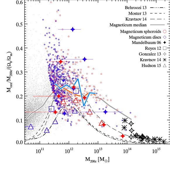
Figure 1: The stellar mass fraction of central galaxies with respect to critical halo mass $M_{200\mathrm{c}}$ normalized by the global, cosmological baryon fraction $\Omega_{b}/\Omega_{m}$, as a function of the halo mass $M_{200\mathrm{c}}$. There is no difference between spheroids (red circles) and discs (blue diamonds).

Over the past years several studies investigated the stellar-to-halo-mass relation (e.g. Mandelbaum et al., 2006; Behroozi et al., 2010; Dutton et al., 2010; Moster et al., 2010; Wake et al., 2011; Munshi et al., 2013; Kravtsov et al., 2014; Brook et al., 2014; Shankar et al., 2014; Rodríguez-Puebla et al., 2015; van Uitert et al., 2016; Tinker et al., 2016). This relation, applicable only for galaxies at the center of the underlying dark matter halo, can give important insight into the galaxy formation process. One interesting question is, for example, if galaxies of identical stellar mass but different morphological type are hosted by dark matter halos of different masses. Another interesting aspect is, that the efficiency with which galaxies are converting their cosmological baryon reservoir into stars, turned out to depend on halo mass, where galaxies residing in dark matter halos of approximately $10^{12}M_{\odot}$ appear to be most efficient.

To investigate this aspect, we show the baryon conversion efficiency as function of halo mass for our central galaxies in Fig. 1, where we show the elliptical galaxies as red circles and the disc galaxies as blue diamonds. Intermediate galaxies and galaxies below our mass cut are shown as gray dots. The gray solid lines mark the median of all galaxies, while the red and blue solid lines show the median of the ellipticals and discs, respectively. For comparison, we over-plot data points from observations by Mandelbaum et al. (2006) (filled stars), Reyes et al. (2012) (squares), Gonzalez et al. (2013) (open stars), Kravtsov et al. (2014) (asterisks) and Hudson et al. (2015) (triangles), where the colours red and blue represent samples of elliptical/early-type galaxies and disc/late-type galaxies, respectively. Our simulated galaxies agree qualitatively with the different observations, which show a wide spread. In both simulations and observations the differences for different galaxy types are only marginal. The differences between our simulations and the observations are most prominent at the low and very high-mass end. They are driven by too inefficient stellar feedback for the low-mass haloes and too inefficient black hole feedback at the high-mass end.

Only at the very high-mass end, X-ray observations allow to infer unambiguously the underlying dark matter potential of individual galaxies (Kravtsov et al., 2014; Gonzalez et al., 2013). In addition, the outer stellar components of these massive galaxies can be measured and their total stellar mass can be inferred, pushing the observations closer to our simulation result. We also plot the curves obtained with abundance matching by Moster et al. (2013) (dashed line), Behroozi et al. (2013) (dash-dotted line), and Kravtsov et al. (2014) (solid line). Especially, the results obtained by Kravtsov et al. (2014) resemble very closely the simulation result.

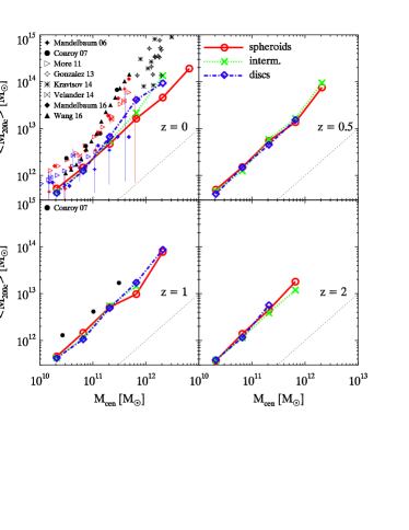
Figure 2: The average critical halo mass $M_{\mathrm{200c}}$ of a halo as a function of the stellar mass of the central galaxy for different redshifts.

A direct comparison between the total mass of the halo and the stellar mass of the central galaxy and its evolution with time is shown in Fig. 2. Red, blue and green lines represent the relation for the ellipticals, discs, and intermediates in the simulation, respectively. At redshift $z=0$ (upper left panel) we add data points from Mandelbaum et al. (2006), Conroy et al. (2007), More et al. (2011), Gonzalez et al. (2013), Kravtsov et al. (2014), Velander et al. (2014), Mandelbaum et al. (2016) and Wang et al. (2016). Black symbols represent those studies that do not distinguish between galaxy types, while red symbols represent elliptical/red/early-type galaxy samples and blue symbols represent spiral/blue/late-type galaxy samples.

At masses below $2\times 10^{11}M_{\odot}$ the simulations overall lie within the large spread covered by the observations. Although the simulations best resemble the results by Mandelbaum et al. (2006, 2016), they generally predict slightly higher stellar mass at given halo masses than most observations. This difference increases with stellar mass. However, at the very high-mass end, where observations can properly include the outermost parts of the galaxies in form of the ICL component (Kravtsov et al., 2014; Gonzalez et al., 2013), the observations lie again closer to our results. Therefore, this systematic upturn seen in the observations could be related to the effect of the contribution of the outer halo to the total stellar mass.

Using observational data from the SDSS Mandelbaum et al. (2006) and More et al. (2011) concluded that the halo mass is independent of the morphology at a fixed stellar mass below $10^{11}$ and $2\cdot 10^{10.5}M_{\odot}$, respectively, while both found that red/elliptical galaxies reside in more massive haloes at higher stellar masses. They argue that this halo mass is likely to reflect the mass of the cluster/group in which more massive ETGs live in. Mandelbaum et al. (2016) find that passive galaxies with stellar masses between $10^{10.3}$ and $10^{11.6}M_{\odot}$ reside in more massive halos than their star-forming counterparts. While our simulations also do not show any differences for the host halo masses at low stellar masses for ellipticals and discs, we cannot support this conclusion that dark matter haloes of spheroids are more massive than those of disc galaxies with comparable stellar masses. In contrast, we even find that disc galaxies with stellar masses above $2\times 10^{11}M_{\odot}$ live in more massive haloes than spheroids of the same stellar mass, however, this could be due to low number statistics, since at high stellar masses there are only few discs in our simulation.

This discrepancy vanishes at higher redshift, where we do not find any differences between the ellipticals and discs, even at large stellar masses. Furthermore, we do not find any evolution of the stellar-to-halo-mass relation with redshift at all, in agreement with observations using satellite kinematics by Conroy et al. (2007), who find that the the stellar to halo mass ratio does not evolve between $z\sim 0$ and $z\sim 1$ for their sample of observed host galaxies below $M_{\mathrm{star}}\approx 1.5\times 10^{11}M_{\odot}$. This is partly in agreement with Hudson et al. (2015) who find no significant redshift evolution for their sample of blue galaxies. However, they observe a time evolution of the relation for their red galaxies.

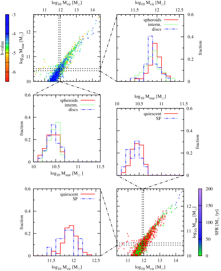
Figure 3: The stellar to halo mass relation for the centrals in Box4 at redshift $z=0$. Top left: the virial mass against the stellar mass of individual centrals, colour-coded by the $b$-value; top right: the fraction of centrals with $M_{\mathrm{star}}\in[2.7\cdot 10^{10},3.3\cdot 10^{10}]$ in bins of $M_{\mathrm{vir}}$, divided into spheroids, intermediates and discs; middle left: the fraction of centrals with $M_{\mathrm{vir}}\in[7.8\cdot 10^{11},9.5\cdot 10^{11}]$ in bins of $M_{\mathrm{star}}$. Bottom right: the virial mass against the stellar mass of individual centrals, colour-coded by the SFR; bottom right: the fraction of centrals with $M_{\mathrm{star}}\in[2.7\cdot 10^{10},3.3\cdot 10^{10}]$ in bins of $M_{\mathrm{vir}}$ divided into quiescent and star-forming; middle right: the fraction of centrals with $M_{\mathrm{vir}}\in[7.8\cdot 10^{11},9.5\cdot 10^{11}]$ in bins of $M_{\mathrm{star}}$.

In Fig. 3 we take a closer look at the stellar-to-halo-mass relation at a fixed stellar and virial mass regarding the different classifications, i.e. the classification according to the kinematical $b$-value and that according to the sSFR, of the central galaxies at $z=0$. The upper left panel shows the relation for individual central galaxies colour-coded by the dynamical classification parameter $b$-value. There is no observable trend with the $b$-value. The upper right panel shows the distribution of the virial masses of the centrals with stellar masses in the small range between $2.7\cdot 10^{10}M_{\odot}$ and $3.3\cdot 10^{10}M_{\odot}$. In agreement with Fig. 2, we find that the spheroidal galaxies peak at higher virial masses than the discs. When looking at the distributions of centrals of virial masses in the range between $7.8\cdot 10^{11}M_{\odot}$ and $9.5\cdot 10^{11}M_{\odot}$ (middle left panel) we do not find a difference in the distribution.

The right bottom panel shows the relation for the galaxies colour-coded by the SFR, where centrals with SFRs $<1M_{\odot}/yr$ are red. As on the upper left panel there is no visible trend between the two quantities and the SFR. In contrast to the result where we have taken the $b$-value (upper right), the same galaxy population in the same small stellar mass bin shows no difference in the distribution in the virial masses of quiescent and star-forming centrals (bottom left). There is also no difference in the distribution of the stellar masses at fixed virial mass (middle right panel), which is in agreement with the results from the $b$-value classification.

This result demonstrates that different classifications can lead to different conclusions regarding the relation between the virial mass and the stellar mass and the morphology. Furthermore, we find a dependence on the mass range: As shown in Fig. 2, at higher mass this trend even reverses. Additionally, we clearly see that a different behaviour occurs if the distribution at fixed stellar mass (where in this case we see a different behaviour) is considered, or the distribution at fixed virial mass (where in this case we do not see a different behaviour) is taken.

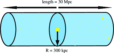
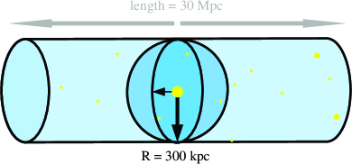
Figure 4: Selecting galaxies in different ways: The upper figure shows illustrates Method 1, where we select satellites within a cylinder of radius $r=300$kpc and a length of 30 Mpc. The lower figure illustrates the second method, where we select all satellites within a sphere of 300kpc.

4 The Abundance of Satellites

In a recent observational study, Ruiz et al. (2015) tried to infer the dark matter halo masses of galaxies based on the abundance of their satellites. They found a systematically decreasing number of satellites around galaxies along the Hubble sequence. As in the observations, we target all galaxies above a given mass threshold in our simulations, regardless of them being centrals or not, and assign all surrounding galaxies within a mass ratio of $M_{\mathrm{sat}}/M_{\mathrm{host}}\in[0.01,1]$ to be their apparent satellite galaxies.

By different ways of counting, as shown in Fig. 4, we can estimate the contribution of projection effects by performing our selection in two different ways: First, we select apparent satellite galaxies within a cylinder of radius $r$ and with a length $l$, as usually done in observations; Second, we select apparent satellite galaxies within a sphere of radius $r$ around a target galaxy.

To obtain a meaningfully statistical number of galaxies we had to choose a mass threshold of $M_{\mathrm{star}}\geq 10^{10}M_{\odot}$, which is lower than the one used by Ruiz et al. (2015). However, in respect to $r$ and $l$ we follow the observations by Wang & White (2012) and Ruiz et al. (2015), namely by choosing a radius $r=300\mathrm{kpc}$ and a length $l=+/-15\mathrm{Mpc}$ along the line of sight, which correspond to the redshift interval of $|\Delta z|<1000\mathrm{kms^{-1}}$.

4.1 Comparison of the Satellite Number with Recent Observations

In the following section we compare the abundance of inferred satellites around the selected sample of galaxies in our simulation with the results from Ruiz et al. (2015). Therefore, we use the first selection method, where the apparent satellites are counted within a cylinder to calculate the number of inferred satellites around massive galaxies.

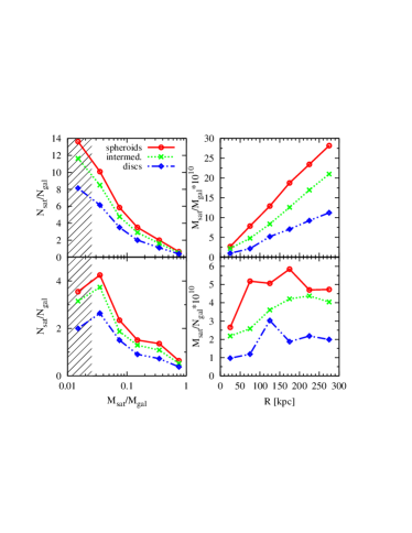
Figure 5: Upper Left: The mass fraction of satellites with respect to the stellar mass of the host galaxies against the cumulative number of satellites per host galaxy in a cylinder of radius $r=300\mathrm{kpc}$ and a length of $30\mathrm{Mpc}$. Lower left: The differential number of satellites per host galaxy. Upper right: The cumulative radial distribution of the satellite mass around host galaxies. Lower right: The differential distribution of the satellite mass along the radius.

In the left panels of Fig. 5 we show the mean number of inferred satellites as function of their stellar mass ratio to the host galaxy at $z=0$. The upper panel shows the (anti-)cumulative fraction, while on the lower panel the differential fraction is shown. The shaded area indicates the completeness of our sample, assuming that galaxies with more than 100 star particles are always numerically resolved. The number of satellites for spheroidal host galaxies is shown in red, while the according numbers for disc host galaxies are shown in blue. In agreement with observations by Ruiz et al. (2015) (see also e.g., Wang et al. (2014)), we find that spheroidal host galaxies have more inferred satellites than disc galaxies.

The radial distribution of the apparent satellite mass around the host at redshift $z=0$ is shown in the right panels of Fig. 5, where the upper one shows the cumulative number, while the lower one shows the differential mass distribution. For all galaxy types the mass in inferred satellites rises towards the outer regions. We find that spheroids are surrounded by $\propto 3$ times the mass in inferred satellites compared to discs and $\propto 1.5$ times compared to intermediates. This tendency agrees qualitatively well with the observations by Ruiz et al. (2015).

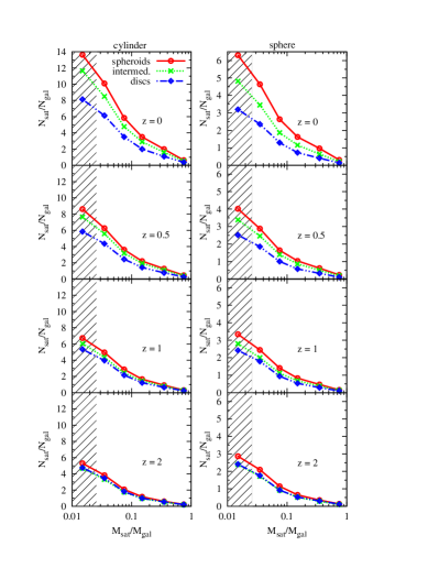
Figure 6: The cumulative number of satellites per host galaxy at different redshifts for all host galaxies. The left column shows the results for a cylinder, while for the right column we collect satellites within a sphere of $r=300\mathrm{kpc}$ (co-moving). The split-up of the distribution is visible for all redshifts, but it becomes smaller with increasing redshift. Be aware: y-axes have different scales!

4.2 Abundance of Satellites for $z>0$

A more reasonable selection (which obviously is not possible in observations) is the second selection method, where the apparent satellites are counted within a sphere around the host galaxy, which is more closely related to the physical satellite population and in principal better allows to study the evolution of the satellite population. As shown in Fig. 6, the different number of inferred satellite galaxies around spheroidal galaxies compared to disc galaxies is already present at higher redshift, independent of the counting method. Interestingly, the relative strength of the signal is even larger when counting apparent satellite galaxies within spheres compared to cylinders, indicating that the immediate environment contributes the most.

The difference of the number of inferred satellites between the spheroids and discs becomes smaller with increasing redshift, due to the decreasing number of inferred satellites around spheroids, while the number of inferred satellites stays constant for disc galaxies. Our results are in agreement with studies by Mármol-Queraltó et al. (2012), Nierenberg et al. (2012) and Nierenberg et al. (2016), who find no significant redshift evolution of the number of apparent satellites for the redshift range between $0.2<z<2$, $0.1<z<0.8$ and $0.1<z<1.5$, respectively. They also mention that the difference in the abundance of inferred satellites between spheroids and disc-like galaxies is more prominent at lower redshift; This likely is an effect of clustering of spheroidal galaxies, which is more important at lower redshifts (see Mármol-Queraltó et al., 2012).

In this context, we want to mention that it is important to keep in mind, in which units the distances are measured, i.e. in physical or co-moving, which becomes more and more important with increasing redshift.

Since it is common to use physical units in observations, we show the result for redshift $z=2$ with physical units in Fig. 18 in the appendix. However, throughout this study we use co-moving units to separate between the expansion of the universe and the real growth of structures.

4.3 Radial Distribution of Satellites

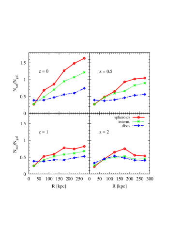
Figure 7: The differential number of satellites per host galaxy depending on the radius of the host galaxies for different redshifts in co-moving units. With increasing redshift the number of satellites decreases, especially for the spheroids.

In Fig. 7 we study how many inferred satellites within a sphere are located in different bins of the radius for four different redshifts. We clearly see that spheroidal galaxies (red circles) have more apparent satellites at all radii than disc galaxies (blue diamonds), except for the inner most region. This is in agreement with studies by Wang et al. (2014) who find similar results for different mass ranges of isolated galaxies from the SDSS. At low redshift (upper left) there is an almost linear distribution of inferred satellites surrounding spheroids, increasing from inside out. While in the inner parts the number of inferred satellites is relatively constant towards higher redshifts, in the outer region the number of inferred satellites decreases with increasing redshift. For intermediates a similar but weaker trend can be seen. In contrast to the spheroids and intermediates, disc galaxies do not have a much ascending slope; the apparent satellites are evenly distributed along the radius and there is no evolution with redshift.

Table 2: The number of central and companion galaxies with stellar masses higher than $10^{10}M_{\odot}$ at four different redshifts

centrals
redshift	$N_{\mathrm{spheroid}}$	$N_{\mathrm{interm.}}$	$N_{\mathrm{disc}}$
0	396	442	481
0.5	344	539	561
1	285	630	629
2	179	663	463
companions
redshift	$N_{\mathrm{spheroid}}$	$N_{\mathrm{interm.}}$	$N_{\mathrm{disc}}$
0	260	318	215
0.5	205	322	254
1	134	304	228
2	67	206	142

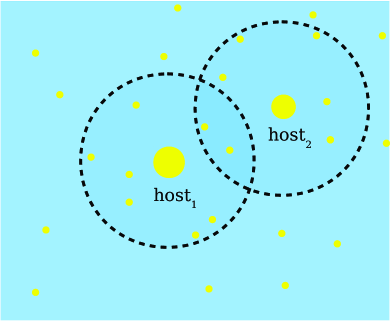
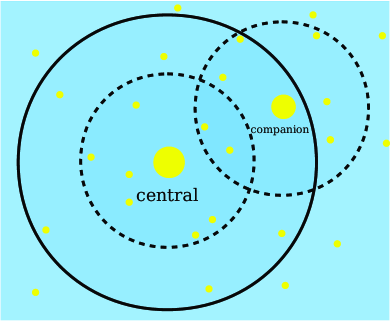
Figure 8: Selecting host galaxies in different ways. The upper figure illustrates the selection of satellites for “all galaxies”: Every galaxy more massive than $10^{10}M_{\mathrm{star}}/M_{\odot}$ is counted as host galaxy. The lower scheme shows the split-up into central and companion galaxies. While host₁ in the upper figure is a central, i.e. the galaxy in the potential minimum of the dark matter halo (black solid circle), host₂ from the upper figure is a companion, i.e. a large satellites within the same dark matter halo.

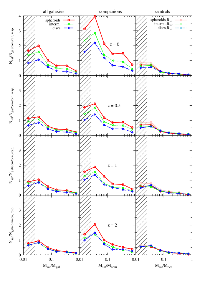
Figure 9: The differential number of satellites per host galaxy at different redshifts (rows) for all host galaxies (left panels), companions (middle panels) and central galaxies (right panels) in co-moving units. The normal colours show satellites within $r=300$kpc, and the pale colours show satellites within $R_{\mathrm{vir}}$. The split-up of the distribution is mainly caused by the companions, since the centrals do not exhibit such a split-up. The split-up in the distribution for the companions is present at all redshifts.

4.4 Comparison of Companions and Centrals

To better understand the origin of the observed signal, we can now split our sample of target galaxies in centrals (which are, as discussed before, at the center of a dark matter halo) and companions, which are by themselves already parts of a larger dark matter halo. Therefore, we count every galaxy from the host galaxy sample as a central galaxy if it resides in the potential minimum of a dark matter halo. All remaining galaxies, which sit within the virial radius of a central galaxy, are considered as companions. This different way of counting compared to what was done before is illustrated in Fig. 8. The resulting numbers of companion and central galaxies classified into spheroids, intermediates and discs at four different redshifts are listed in Table 2.

Fig. 9 shows the number of satellite galaxies inferred for all host galaxies (left column) compared to the number of satellite galaxies for the sample split into centrals (right panel) and companions (middle panel). We see a clear difference in the number of apparent satellites: While there is a clear split-up between spheroidal and disc galaxies for the host and companion samples, there is no such difference visible for the centrals.

Thus, we clearly see that the companions within the sample are responsible for the split-up seen for the sample of all host galaxies. This can be explained by the fact that companions are by definition in dense regions and due to the morphology-density-relation preferentially are spheroidal galaxies. Therefore, we conclude that the observed difference in the apparent number of inferred satellite galaxies around spheroidal and disc galaxies is entirely driven by the morphology-density-relation and not by different underlying halo masses.

This also explains the weakening of the signal with increasing redshift, as shown in the lower panels of Fig. 9 and in Fig. 6. This is caused by the lack of massive companion galaxies at higher redshifts as can clearly be seen from Table 2 and the middle and right panels of Fig. 9. Thus, the split-up of the distributions of companions is visible at all redshifts but less pronounced at higher redshift.

This is also supported by the radial distribution of satellites as previously shown in Fig. 7 (and in Fig. 17, separately for centrals and companions): The spheroidal host galaxies have more satellites than the discs and the number of these satellites increases towards larger radii, again pointing towards the density-morphology-relation as origin of the split up.

4.5 Average Number of Satellites in Dependence of the Virial Mass

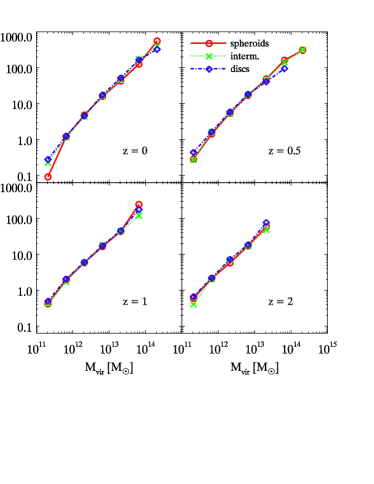
Figure 10: The average number of satellites with stellar masses larger than $10^{8}M_{\odot}$ around centrals, within the virial radius in bins of the virial mass for different redshifts.

In order to see if one can directly infer the halo mass of a central galaxy from the number of the satellites, we show in Fig. 10 the number of satellites averaged for the central galaxies according to their virial mass. Here, we include all satellites with stellar masses higher than $10^{8}M_{\odot}$ that reside within the virial radius of their central galaxy. We find that the number of satellites is directly proportional to the virial mass of the central galaxy, where the central galaxies which reside in halos with higher masses have more satellites than those residing in low-mass halos. There is no difference for galaxies with different morphological types. In addition, we do not find an evolution with redshift.

The independence of the number of satellites of the central’s morphology and the redshift is also shown in Fig. 9, where we included the satellite counts within $R_{\mathrm{vir}}$ in pale colours in the right panels. The change compared to the number of satellites within $r=300\mathrm{kpc}$ is only marginal, since the average virial radius of the central galaxies has about the same size as the considered sphere.

We conclude that counting the satellites of galaxies without distinguishing between central galaxies and companions, i.e. large satellites, just reflects the environment they live in. The number of satellites within the virial radius of centrals, however, remains almost constant with increasing redshift and therefore traces the underlying dark matter halo.

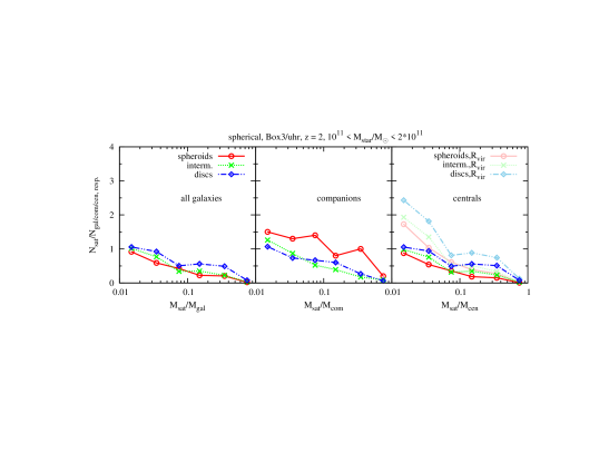
Figure 11: From left to right: same as Fig. 9 but in the larger Box3 with the same resolution at $z=2$. There is no split-up of the distribution for all host galaxies (left panel), since the number of companions is very small in this mass range at $z=2$ and thus the distribution for all galaxies is reflecting that of the centrals (right panel). The distribution of the companions exhibits again the split-up (middle panel).

Table 3: The number of all host galaxies with stellar masses higher between $10^{11}M_{\odot}$ and $2\cdot 10^{11}M_{\odot}$ at $z=2$ in Box3/uhr

galaxy type	$N_{\mathrm{spheroid}}$	$N_{\mathrm{interm.}}$	$N_{\mathrm{disc}}$
all galaxies	156	209	180
companion	10	23	15
central	146	186	165

4.6 Massive Galaxies at High Redshift

In order to test the signal for massive galaxies in more detail by choosing a very narrow mass range of $10^{11}M_{\odot}$ and $2\cdot 10^{11}M_{\odot}$, as done in the observations by Ruiz et al. (2015), we now select galaxies from the larger volume simulation Box3. This large volume simulation was so far only evolved down to a redshift of $z=2$. This simulation has the same resolution as the simulation used before, and we find the same results for the satellite fractions using the full mass range. This volume is actually large enough to obtain several hundreds of galaxies, even within such a narrow mass range, which we can split into companion and central galaxies and classify them as spheroids, intermediates, and discs, as reported in Table 3. Note that the underlying AGN feedback in this new, larger volume simulation has slightly different parameters, which generally leads to a fraction of passive galaxies even closer to the observed one, as shown in Steinborn et al. (2015).

In Fig. 11 we plot the mass fraction of the satellites against the number per host galaxy as in Fig. 9 but for the narrow mass range of $10^{11}M_{\odot}$ and $2\cdot 10^{11}M_{\odot}$, where our simulation resolves the complete mass range of the satellite galaxies. We still see the increased number of satellites for elliptical companions, and no increased number for centrals. As shown before, at this high mass range, the signal for the centrals even slightly reverses. The pale curves again show the satellite number per central within the virial radius. From this we conclude that our key result, namely that the split-up is caused by the companion galaxies, is not biased by a mass selection effect, since we find this split-up in both galaxy samples despite the different mass ranges.

5 Relation between Host and Satellite Properties

Until now we have only considered the number of satellites for centrals of different morphology. However, at high redshift morphology (traced via kinematic properties like the $b$-value) and starforming activity can mean different things, as shown before (see also Teklu et al., 2015). Additionally, the relation between satellites and their centrals seems to be more complex. Therefore, it is important to understand the connection between properties of host and satellite galaxies in more detail. In the following section we will take a closer look at the relations between host and satellite galaxies with respect to their star formation rates, formation redshifts, and dynamical properties.

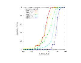
Figure 12: The cumulative fraction of centrals binned according to their SFR in Box3 at $z=2$. The formation redshift of the centrals is colour-coded, where younger centrals are blue and older ones are red. There is a trend that young centrals have a higher SFR than older ones.

5.1 SFR and Formation Redshift of Satellites and Central Galaxies

In Fig. 12 we show, how the current star formation rate is reflected in the formation redshift ($z_{\mathrm{form}}$). To avoid bias from possible mass-dependence effects, we therefore again analyse the centrals from the narrow mass range $[10^{11},2\cdot 10^{11}]M_{\odot}$. Here we show the cumulative fraction of centrals according to their star formation rate at $z=2$, where the colours represent the average redshift, where the stars of a given galaxy were formed. As expected, we clearly find a smooth, continuous tendency for older (red) centrals to have lower star formation rates at current time (e.g. $z=2$), and therefore older centrals are more quenched than younger (blue) centrals.

In the following we want to verify if and how the $b$-value (i.e., the morphology), the star formation rate, and the formation redshift of the central galaxies correlate with the formation redshift and the star formation of their satellite galaxies (within the virial radius).

The left column of Fig. 13 always shows the cumulative fraction of the star formation of the satellite galaxies, while the right column always shows the cumulative fraction of the formation redshift of the satellite galaxies. The different colours in the rows reflect different selection criteria of the underlying central galaxies as follows:

The upper row shows the sample of host galaxies split into the different morphological types (e.g. spheroids, intermediates and discs classified via low, medium and high $b$-values, respectively). For all host morphologies, the majority of satellite galaxies are already quenched and do not show any differences in their formation time. The curves for the star formation rates for satellites of the disc-like and spheroidal centrals are indistinguishable above $0.1M_{\odot}/yr$, and a KS-test gives a probability of $5.36\cdot 10^{-1}$ that the overall distributions (red and blue curve) are the same.

In the middle panels we check how the star formation of the centrals is related to the star formation and the formation redshift of their satellites. The left panel shows that centrals with almost no star formation (red curve) are mainly surrounded by satellites which themselves have no star formation, while star-forming centrals have a larger fraction of satellites with significant star formation. This suggests that the environment provides the star-forming centrals as well as their satellites continuously with gas. Additionally, we see an indication for a weak correlation between the star formation of the centrals and the formation redshift of their satellites (right panel). Here, the KS-test gives a probability of $2.14\cdot 10^{-2}$ that the two distributions of non-star-forming (red curve) and highly star-forming (purple curve) centrals have the same underlying distribution.

In the lower row we colour-code the distributions according to the formation redshift of the centrals. On the left panel we note a slight correlation between the star formation of the satellites and the formation redshift of the centrals: Older central galaxies have a larger fraction of quiescent satellites, younger centrals have a larger fraction of star-forming satellites, except for the bin with the youngest centrals (blue curve) which, however, is based on low number statistics. On the right panel we find a correlation between the formation redshift of the satellites and the formation redshift of their centrals. The older centrals (red curve) have older satellites, while the younger centrals (blue curve) tend to have younger satellites, which is confirmed by the KS-test with a probability of $1.85\cdot 10^{-6}$.

We conclude that the morphology of the central galaxy does not relate to the star formation and the formation redshift of its satellites at $z=2$. Nevertheless, we find a significant correlation between the star formation and the formation redshift of the centrals themselves with the star formation and the formation redshift of their satellites, reflecting the so-called conformity (see e.g. Tinker et al., 2017). The fact that there is neither a correlation between the $b$-value of the central and the star formation and formation redshift of the satellites nor a correlation between the $b$-value and the number of satellites suggests that the environment is the main mechanism that controls the global star formation properties and thus links the formation redshift of both centrals and satellites.

5.2 Evolution of the SFR-$z_{\rm{form}}$ relation

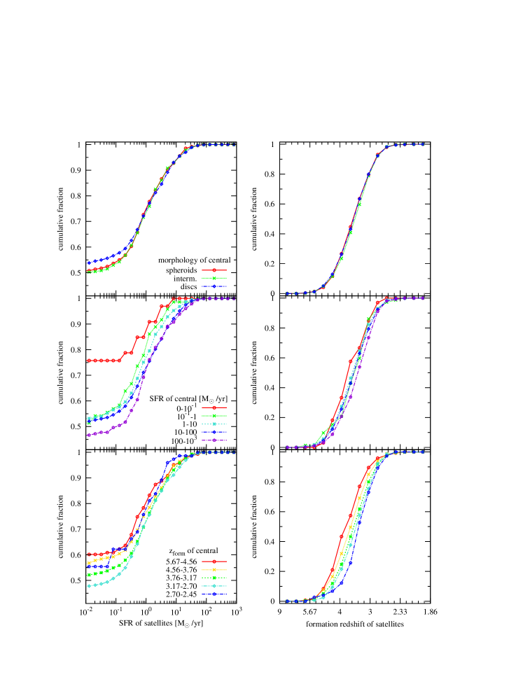
Figure 13: Left: The cumulative fraction of satellites within the virial radii of centrals binned according to their SFR. Right: The cumulative fraction of satellites according to their formation redshift. In the upper row the colour encodes the $b$-value of the centrals of the satellites, the middle row divides the centrals according to the SFR and the lower panels show the satellite population split according to the formation redshift of their central, for galaxies in Box3 at $z=2$.

The evolution of the relation between the star formation rate and the formation redshift of the central galaxies is shown in Fig 14. Here all panels show a scatter plot of the star formation rate as function of formation redshift, coloured by the stellar mass of the central. The left and middle panels present the $z=2$ results for the narrow mass range sample from Box3 (left) and the full sample from the smaller Box4 simulation (middle). The right panel shows the according result from Box4 at $z=0$. The green diamonds are the averaged star formation rate, binned for different formation redshifts. Centrals with star formation rates lower than $0.01M_{\odot}/yr$ are plotted on the lowest displayed value of the $y$-axis.

We find a clear trend of the median star formation rate with the formation redshift at $z=2$, in agreement with our previous finding that old centrals tend to have a lower star formation rate, while young centrals on average have a higher star formation rate. A part of this relation is expected, as more massive galaxies are expected to have higher star formation rates and also form earlier. However, this relation holds even at fixed stellar mass, as shown by the narrow mass range sample (left panel in Fig. 14). This means that galaxies with already quenched star formation usually have formed earlier, in line with previous studies by e.g. Feldmann et al. (2016). At $z=2$ we find a median formation redshift for star-forming galaxies to be 3.36, which is in line with recent observations by Thomas et al. (2016), who evaluate a median formation redshift of $\sim 3.22$ for their galaxy sample observed at $2<z<6.5$ when using a formation redshift based on mean stellar ages similar to ours.

At redshift $z=0$ (right panel), we still find this correlation between the formation redshift $z_{\mathrm{form}}$ and the star formation rate for low-mass galaxies, while high-mass galaxies show no clear trend anymore. These massive galaxies live in very dense environments like galaxy groups and clusters in which star formation can continue, fed by cooling from the halo, even for systems with early formation times. Such massive galaxies at $z=0$ all have formed at early times, typically with a formation redshift between $z=1.5$ and $z=2.5$.

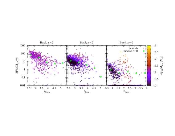
Figure 14: The formation redshift $z_{\mathrm{form}}$ against the current SFR for centrals with stellar masses between $10^{11}$ and $2\cdot 10^{11}M_{\odot}$ in Box3 at $z=2$ (left) and centrals with stellar masses above $10^{10}M_{\odot}$ in Box4 at $z=2$ (middle) and at $z=0$ (right).

Table 4: The number of centrals and companions with $M_{\mathrm{star}}>10^{10}M_{\odot}$ divided into quiescent and star-forming at four different redshifts

	centrals		companions
redshift	$N_{\mathrm{quiescent}}$	$N_{\mathrm{SF}}$	$N_{\mathrm{quiescent}}$	$N_{\mathrm{SF}}$
0	1069	250	694	99
0.5	1064	380	633	148
1	908	636	466	200
2	107	1198	73	242

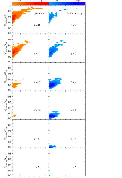
Figure 15: The fraction of quiescent galaxies more massive than $10^{8}M_{\odot}$ within a sphere of radius 5 Mpc (co-moving) around quiescent (left panels) and star-forming (right panels) centrals with stellar masses above $10^{10}M_{\odot}$ in Box4 at different redshifts. There is a clear build-up of the density-morphology-relation starting at around $z=2$; while at high redshift the fraction of quiescent galaxies does not depend on the number of neighbouring galaxies, i.e. the environment, with decreasing redshift the environment becomes more and more important for the quiescent fraction. The distribution looks very similar for quiescent and star-forming galaxies.

5.3 The Relation between the Environment and the Star Formation Rate

To investigate how the environment is affecting the star formation rate of galaxies, we characterize the environment of galaxies by their neighbour counts. Therefore, we count all galaxies with stellar masses above $10^{8}M_{\odot}$ within a sphere of radius $r=5~{}{\rm{Mpc}}$ around our centrals. We define the environmental density as

$$\rho_{\mathrm{env}}=\frac{N_{\mathrm{gal}}(5Mpc)}{4/3\cdot\pi\cdot r^{3}}.$$ (2)

Here, following Treu et al. (2003), the radius was chosen to include all potential cluster members. Accordingly, using the distance to the 10th neighbour results in a similar median value (see Cappellari et al., 2011).

Fig. 15 shows the build-up of the density-morphology-relation (e.g. Dressler, 1980) with cosmic time. The different panels show the dependence of the density-morphology-relation on the star formation properties of the central galaxies: The left panels show the quiescent centrals, while the right panels show the star-forming centrals. Table 4 lists the sample sizes at the different redshifts.

We do not find evidence for a density-morphology-relation at high redshift ($z>2$), for neither of the two galaxy types. Generally, we see a clear evolution with decreasing redshift, and the build-up of the density-morphology-relation starts at around $z=2$. At this redshift the trend appears that centrals that live in over-dense regions have a high fraction of quiescent neighbours, while galaxies in lower density environments have on average a lower fraction of quiescent neighbours. This trend is in good agreement with observations by Darvish et al. (2016), who also find that at higher redshift the fraction of quiescent galaxies does not depend on the environment, while it does at low redshift. Interestingly, it does not make a difference if the central is quiescent or star-forming itself: There are for example quiescent centrals in low-density environments that have a very low fraction of quiescent galaxies around them and vice versa, star-forming centrals in high-density environments with a high fraction of quiescent galaxies.

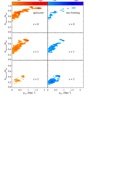
Figure 16: The same as in Fig. 15, but for companions. As seen for the centrals, there is a built-up of the density-morphology-relation, where there is no difference between quiescent and star-forming companions.

Several studies (e.g., Peng et al. (2010), Lee et al. (2015) and Hirschmann et al. (2016)) find that this environmental quenching is important especially for low-mass satellite galaxies. For completeness, we show in Fig. 19 of the Appendix the density-morphology-relation for centrals in physical units.

In Fig. 16 we show the density-morphology-relation for the companion galaxies for redshifts $z=0$ to $z=2$, as there are too few companions at higher redshifts. The shape of the density-morphology-relation for the companion galaxies is the same as for the central galaxies (see Fig. 15). Similarly, it does not make a difference for the fraction of quiescent neighbouring galaxies if the companion galaxy itself is quiescent or star-forming. While the number density of the quiescent central galaxies peaks in the low-density environments, the number density of the quiescent companions is more shifted towards denser environment. In contrast, the distribution of the number densities in the density-morphology-relation of star-forming centrals and satellites does not differ. This clearly demonstrates that environmental quenching is more important for satellite galaxies than for centrals. Since our satellite galaxies on average are low-mass galaxies this supports earlier studies by Hirschmann et al. (2016), who concluded that the fraction of quiescent galaxies is mainly determined by internal processes, while the environment becomes important at lower masses.

6 Discussion and Conclusions

We use galaxies extracted from the high resolution cosmological simulation suite Magneticum to investigate the relation between the dark matter halo mass and the internal properties of galaxies as well as the environmental imprint on the star formation properties. Especially, we want to test whether the morphological type of a galaxy depends on the dark matter halo mass, as recently concluded from the observed differences in the abundance of satellites around galaxies of different morphological types by Ruiz et al. (2015). We select all galaxies with stellar masses above $10^{10}M_{\odot}$ and use a dynamical parameter, the so-called $b$-value (see Teklu et al., 2015), as indicator of morphological type. We find that:

• When applying the observed strategy of counting satellite galaxies around all massive galaxies we clearly reproduce the observed signal of more satellites around spheroidal galaxies compared to disc galaxies for both the total numbers for different mass ratios as well as for the radial abundance profile.

• This signal does not depend on (and therefore is not produced by) the way of defining the volume in which the satellites are counted. We find that the signal even holds if we use spherical volumes around the galaxies instead of a cylinder defined by a redshift range as observers have to rely on.

• However, when splitting the sample of massive galaxies into galaxies at the centre of their dark matter halo (i.e. centrals) and companion galaxies (which are only large satellites of other massive galaxies within a common dark matter potential), we find that the signal is exclusively caused by the companion galaxies. If only the central galaxies are considered, the signal completely disappears.

• This result is found to hold true even at higher redshifts up to $z=2$. However, when considering all galaxies (centrals and companions), the difference in the satellite number between spheroids and discs becomes smaller with increasing redshift due to the lower number of companions at higher redshift.

• This is also supported by the fact that the baryon conversion efficiency of our galaxies does not show any significant trend with the inferred morphological type.

We therefore conclude that the observed differences in the abundance of satellites around massive galaxies of different morphological types is only driven by the different environments, in which spheroid and disc galaxies are typically living, and that they are not related to differences in the baryon conversion efficiency of galaxies with different morphological types. This is supported by observational results from Guo et al. (2015) that isolated primaries in a filamentary environment have more satellites than those outside of filaments.

We investigate in more detail the relation between the quenching of star formation and our morphological classification based on the $b$-value for galaxies at high redshift (i.e. $z=2$). Selecting a large number of galaxies ($\approx 500$) within a very narrow mass range (i.e. $10^{11}M_{\odot}<M_{\mathrm{star}}<2\cdot 10^{11}M_{\odot}$), allows us to exclude any mass dependencies. We find that:

• In contrast to galaxies at $z=0$, the galaxies which are already quenched at $z=2$ do not show a relation to their morphological type.

• Quenched galaxies at $z=2$ have on average formed earlier than their starforming counterparts, as suggested in previous studies (e.g. Feldmann et al., 2016).

• Satellites of quenched galaxies at $z=2$ have typically formed earlier and show on average less star formation activity compared to satellites of star-forming galaxies, as suggested in earlier studies (e.g. Feldmann et al., 2016).

Our simulations furthermore show that at redshifts of $z=2$, in contrast to present time, the dynamical classification of galaxies based on morphology results in a different selection than the classification based on star formation. Our results are broadly in agreement with the picture that was pointed out in previous studies (e.g. Peng et al., 2010; Hirschmann et al., 2016; Huertas-Company et al., 2016) that the environment is effective in quenching star formation of lower mass galaxies, while at higher masses and redshifts $z>1$ other (internal) effects are the dominant drivers.

Additionally, we study the connection between the environment and the star formation rate evaluating the environment density $\rho_{\mathrm{env}}$. From the evolution of the density-morphology-relation between $z\approx 5$ and $z=0$ we conclude that:

• At high redshifts ($z\geq 3$) there is no signature of a density-morphology-relation for central galaxies. The built-up of the density-morphology-relation starts at around $z\approx 2$.

• The density-morphology-relation for quiescent and starforming centrals is similar, indicating a negligible influence of the environment on the star-forming properties of the central galaxies.

• The shape of the density-morphology-relation for the companion galaxies is the same as for the central galaxies.

• The quiescent fraction of companion galaxies is comparable to that of the central galaxies.

• The number density of the quiescent central galaxies peaks in the low-density environments, while the number density of the quiescent companions peaks at denser environments.

• The distribution of the number densities in the density-morphology-relation of star-forming centrals and satellites does not differ.

We conclude that environmental quenching is more important for satellite galaxies than for centrals.

Appendix A The Radial Distribution of Satellites

Previously we showed the apparent difference in the radial profiles of satellite abundance around spheroidal and disc-like galaxies, where spheroidal galaxies have more satellites than disc-like host galaxies (Fig. 7). We demonstrated that this split-up is caused by the companion galaxy population (see middle and right panels Fig. 9). In Fig. 17 we demonstrate that this difference in the radial distribution of satellites around the host galaxies also originates purely from the companions (right panel), while the signal completely disappears for the central galaxies (left panel), as expected.

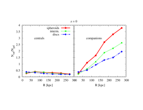
Figure 17: The differential radial distribution of satellites per host galaxy at redshift $z=0$ for centrals (left) and companions (right).

Appendix B The World in Physical Units

Since it is common to use physical units in observations, we show some of our results in physical units, where we take the expansion of the Universe into account. The difference to the co-moving units, which capture the real growth of a structure, becomes more and more important with increasing redshift.

B.1 Satellite Fraction in Physical Units

In Fig. 9 we showed the abundance of satellites per host galaxy binned by the mass ratio with respect to their host, for all potential host galaxies (left panel) and split into companion (middle panel) and central (right panel). Fig. 18 shows the same for redshift $z=2$ in physical units. Compared to the bottom panels in Fig. 9, the number of satellite galaxies is higher. It is also higher than at $z=0$, which is not surprising when comparing volume-limited samples at different redshifts (see also discussion in Conroy et al. (2007)). This demonstrates that careful choice of distance scale is important, especially at high redshift.

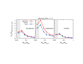
Figure 18: The differential number of satellites per host galaxy at redshift $z=2$ for all host galaxies (left), companions (middle) and central galaxies (right) within a sphere of 300 kpc in physical units, binned according to their mass ratio.

B.2 Density-Morphology-Relation in Physical Units

The influence of the choice of distance scale becomes especially prominent for the density-morphology-relation. Comparing Fig. 15, which illustrates the density-morphology-relation for centrals in co-moving units, with Fig. 19, which is the same relation in physical units, the shape and its evolution look strikingly different. When taking a sphere in physical units, the induced change in the distance scale masks the presence of the density morphology relation at $z\geq 1$, resulting in a later and steeper increase of the density-morphology-relation. This is due to the fact that in physical units the search radius becomes larger compared to the central galaxies with increasing redshift and we thus go farther outside of the “local” environment to the “global” environment. In the “local” environment we find a higher number of quiescent neighbouring galaxies than in the “global” environment, emphasizing the importance of the “local” environment for the satellite quenching.

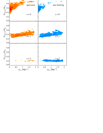
Figure 19: The fraction of quiescent galaxies more massive than $10^{8}M_{\odot}$ within a sphere of radius 5 Mpc (physical) around quiescent (left panels) and star-forming (right panels) centrals with stellar masses above $10^{10}M_{\odot}$ in Box4 at different redshifts.

References

- Abadi et al. (1999) Abadi M. G., Moore B., Bower R. G., 1999, MNRAS, 308, 947
- Abramson et al. (2011) Abramson A., Kenney J. D. P., Crowl H. H., Chung A., van Gorkom J. H., Vollmer B., Schiminovich D., 2011, AJ, 141, 164
- Arth et al. (2014) Arth A., Dolag K., Beck A. M., Petkova M., Lesch H., 2014, preprint, (arXiv:1412.6533)
- Beck et al. (2015) Beck A. M., et al., 2015, preprint, (arXiv:1502.07358)
- Behroozi et al. (2010) Behroozi P. S., Conroy C., Wechsler R. H., 2010, ApJ, 717, 379
- Behroozi et al. (2013) Behroozi P. S., Wechsler R. H., Conroy C., 2013, ApJ, 770, 57
- Boissier et al. (2012) Boissier S., et al., 2012, A&A, 545, A142
- Brook et al. (2014) Brook C. B., Di Cintio A., Knebe A., Gottlöber S., Hoffman Y., Yepes G., Garrison-Kimmel S., 2014, ApJ, 784, L14
- Brouwer et al. (2016) Brouwer M. M., et al., 2016, preprint, (arXiv:1604.07233)
- Bundy et al. (2009) Bundy K., Fukugita M., Ellis R. S., Targett T. A., Belli S., Kodama T., 2009, ApJ, 697, 1369
- Cappellari et al. (2011) Cappellari M., et al., 2011, MNRAS, 416, 1680
- Conroy et al. (2007) Conroy C., et al., 2007, ApJ, 654, 153
- Darvish et al. (2016) Darvish B., Mobasher B., Sobral D., Rettura A., Scoville N., Faisst A., Capak P., 2016, preprint, (arXiv:1605.03182)
- Davis et al. (1985) Davis M., Efstathiou G., Frenk C. S., White S. D. M., 1985, ApJ, 292, 371
- Dolag et al. (2004) Dolag K., Jubelgas M., Springel V., Borgani S., Rasia E., 2004, ApJ, 606, L97
- Dolag et al. (2005) Dolag K., Vazza F., Brunetti G., Tormen G., 2005, MNRAS, 364, 753
- Dolag et al. (2009) Dolag K., Borgani S., Murante G., Springel V., 2009, MNRAS, 399, 497
- Dolag et al. (2015) Dolag K., Komatsu E., Sunyaev R., 2015, preprint, (arXiv:1509.05134)
- Donnert et al. (2013) Donnert J., Dolag K., Brunetti G., Cassano R., 2013, MNRAS, 429, 3564
- Dressler (1980) Dressler A., 1980, ApJ, 236, 351
- Dutton et al. (2010) Dutton A. A., Conroy C., van den Bosch F. C., Prada F., More S., 2010, MNRAS, 407, 2
- Eke et al. (1996) Eke V. R., Cole S., Frenk C. S., 1996, MNRAS, 282, 263
- Erfanianfar et al. (2016) Erfanianfar G., et al., 2016, MNRAS, 455, 2839
- Fabjan et al. (2010) Fabjan D., Borgani S., Tornatore L., Saro A., Murante G., Dolag K., 2010, MNRAS, 401, 1670
- Fall (1983) Fall S. M., 1983, in Athanassoula E., ed., IAU Symposium Vol. 100, Internal Kinematics and Dynamics of Galaxies. pp 391–398
- Feldmann et al. (2016) Feldmann R., Hopkins P. F., Quataert E., Faucher-Giguère C.-A., Kereš D., 2016, MNRAS, 458, L14
- Franx et al. (2008) Franx M., van Dokkum P. G., Förster Schreiber N. M., Wuyts S., Labbé I., Toft S., 2008, ApJ, 688, 770
- Gonzalez et al. (2013) Gonzalez A. H., Sivanandam S., Zabludoff A. I., Zaritsky D., 2013, ApJ, 778, 14
- Gunn & Gott (1972) Gunn J. E., Gott III J. R., 1972, ApJ, 176, 1
- Guo et al. (2013) Guo Q., Cole S., Eke V., Frenk C., Helly J., 2013, MNRAS, 434, 1838
- Guo et al. (2015) Guo Q., Tempel E., Libeskind N. I., 2015, ApJ, 800, 112
- Hernquist (1989) Hernquist L., 1989, Nature, 340, 687
- Hirschmann et al. (2014) Hirschmann M., Dolag K., Saro A., Bachmann L., Borgani S., Burkert A., 2014, MNRAS, 442, 2304
- Hirschmann et al. (2016) Hirschmann M., De Lucia G., Fontanot F., 2016, MNRAS,
- Hudson et al. (2015) Hudson M. J., et al., 2015, MNRAS, 447, 298
- Huertas-Company et al. (2016) Huertas-Company M., et al., 2016, preprint, (arXiv:1606.04952)
- Komatsu et al. (2011) Komatsu E., et al., 2011, ApJS, 192, 18
- Kravtsov et al. (2014) Kravtsov A., Vikhlinin A., Meshscheryakov A., 2014, preprint, (arXiv:1401.7329)
- Larson et al. (1980) Larson R. B., Tinsley B. M., Caldwell C. N., 1980, ApJ, 237, 692
- Leauthaud et al. (2012) Leauthaud A., et al., 2012, ApJ, 744, 159
- Lee et al. (2015) Lee S.-K., Im M., Kim J.-W., Lotz J., McPartland C., Peth M., Koekemoer A., 2015, ApJ, 810, 90
- Liu et al. (2011) Liu L., Gerke B. F., Wechsler R. H., Behroozi P. S., Busha M. T., 2011, ApJ, 733, 62
- López-Sanjuan et al. (2012) López-Sanjuan C., et al., 2012, A&A, 548, A7
- Mamon (1992) Mamon G. A., 1992, ApJ, 401, L3
- Mandelbaum et al. (2006) Mandelbaum R., Seljak U., Kauffmann G., Hirata C. M., Brinkmann J., 2006, MNRAS, 368, 715
- Mandelbaum et al. (2016) Mandelbaum R., Wang W., Zu Y., White S., Henriques B., More S., 2016, MNRAS, 457, 3200
- Mármol-Queraltó et al. (2012) Mármol-Queraltó E., Trujillo I., Pérez-González P. G., Varela J., Barro G., 2012, MNRAS, 422, 2187
- McDonald et al. (2014) McDonald M., et al., 2014, ApJ, 794, 67
- Mitchell et al. (2015) Mitchell P., Lacey C., Baugh C., Cole S., 2015, preprint, (arXiv:1510.08463)
- More et al. (2011) More S., van den Bosch F. C., Cacciato M., Skibba R., Mo H. J., Yang X., 2011, MNRAS, 410, 210
- Moster et al. (2010) Moster B. P., Somerville R. S., Maulbetsch C., van den Bosch F. C., Macciò A. V., Naab T., Oser L., 2010, ApJ, 710, 903
- Moster et al. (2013) Moster B. P., Naab T., White S. D. M., 2013, MNRAS, 428, 3121
- Munshi et al. (2013) Munshi F., et al., 2013, ApJ, 766, 56
- Nierenberg et al. (2012) Nierenberg A. M., Auger M. W., Treu T., Marshall P. J., Fassnacht C. D., Busha M. T., 2012, ApJ, 752, 99
- Nierenberg et al. (2016) Nierenberg A. M., Treu T., Menci N., Lu Y., Torrey P., Vogelsberger M., 2016, preprint, (arXiv:1603.01614)
- Obreschkow et al. (2015) Obreschkow D., et al., 2015, ApJ, 815, 97
- Peng et al. (2010) Peng Y.-j., et al., 2010, ApJ, 721, 193
- Planck Collaboration et al. (2013) Planck Collaboration et al., 2013, A&A, 550, A131
- Remus et al. (2013) Remus R.-S., Burkert A., Dolag K., Johansson P. H., Naab T., Oser L., Thomas J., 2013, ApJ, 766, 71
- Remus et al. (2016) Remus R.-S., Dolag K., Naab T., Burkert A., Hirschmann M., Hoffmann T. L., Johansson P. H., 2016, preprint, (arXiv:1603.01619)
- Reyes et al. (2012) Reyes R., Mandelbaum R., Gunn J. E., Nakajima R., Seljak U., Hirata C. M., 2012, MNRAS, 425, 2610
- Rodríguez-Puebla et al. (2015) Rodríguez-Puebla A., Avila-Reese V., Yang X., Foucaud S., Drory N., Jing Y. P., 2015, ApJ, 799, 130
- Romanowsky & Fall (2012) Romanowsky A. J., Fall S. M., 2012, ApJS, 203, 17
- Ruiz et al. (2015) Ruiz P., Trujillo I., Mármol-Queraltó E., 2015, MNRAS, 454, 1605
- Shankar et al. (2014) Shankar F., et al., 2014, ApJ, 797, L27
- Spitzer (1962) Spitzer L., 1962, Physics of Fully Ionized Gases
- Springel (2000) Springel V., 2000, MNRAS, 312, 859
- Springel (2005) Springel V., 2005, MNRAS, 364, 1105
- Springel & Hernquist (2003) Springel V., Hernquist L., 2003, MNRAS, 339, 289
- Springel et al. (2001a) Springel V., Yoshida N., White S. D. M., 2001a, Nature, 6, 79
- Springel et al. (2001b) Springel V., White S. D. M., Tormen G., Kauffmann G., 2001b, MNRAS, 328, 726
- Springel et al. (2005) Springel V., Di Matteo T., Hernquist L., 2005, MNRAS, 361, 776
- Steinborn et al. (2015) Steinborn L. K., Dolag K., Hirschmann M., Prieto M. A., Remus R.-S., 2015, MNRAS, 448, 1504
- Steinborn et al. (2016) Steinborn L. K., Dolag K., Comerford J. M., Hirschmann M., Remus R.-S., Teklu A. F., 2016, MNRAS, 458, 1013
- Teklu et al. (2015) Teklu A. F., Remus R.-S., Dolag K., Beck A. M., Burkert A., Schmidt A. S., Schulze F., Steinborn L. K., 2015, ApJ, 812, 29
- Teklu et al. (2016) Teklu A. F., Remus R.-S., Dolag K., 2016, in The Interplay between Local and Global Processes in Galaxies,.
- Thomas et al. (2016) Thomas R., et al., 2016, preprint, (arXiv:1602.01841)
- Tinker et al. (2016) Tinker J. L., et al., 2016, preprint, (arXiv:1607.04678)
- Tinker et al. (2017) Tinker J. L., Hahn C., Mao Y.-Y., Wetzel A. R., Conroy C., 2017, preprint, (arXiv:1702.01121)
- Tonnesen & Cen (2015) Tonnesen S., Cen R., 2015, ApJ, 812, 104
- Tornatore et al. (2004) Tornatore L., Borgani S., Matteucci F., Recchi S., Tozzi P., 2004, MNRAS, 349, L19
- Tornatore et al. (2007) Tornatore L., Borgani S., Dolag K., Matteucci F., 2007, MNRAS, 382, 1050
- Treu et al. (2003) Treu T., Ellis R. S., Kneib J.-P., Dressler A., Smail I., Czoske O., Oemler A., Natarajan P., 2003, ApJ, 591, 53
- Velander et al. (2014) Velander M., et al., 2014, MNRAS, 437, 2111
- Vollmer et al. (2012) Vollmer B., Wong O. I., Braine J., Chung A., Kenney J. D. P., 2012, A&A, 543, A33
- Wake et al. (2011) Wake D. A., et al., 2011, ApJ, 728, 46
- Wang & White (2012) Wang W., White S. D. M., 2012, MNRAS, 424, 2574
- Wang et al. (2014) Wang W., Sales L. V., Henriques B. M. B., White S. D. M., 2014, MNRAS, 442, 1363
- Wang et al. (2016) Wang L., Li C., Jing Y. P., 2016, ApJ, 819, 58
- White (1978) White S. D. M., 1978, MNRAS, 184, 185
- van Uitert et al. (2016) van Uitert E., et al., 2016, MNRAS, 459, 3251