A numerical study of the homogeneous elliptic equation with fractional order boundary conditions

Abstract.

We consider the homogeneous equation ${\mathcal{A}}u=0$, where ${\mathcal{A}}$ is a symmetric and coercive elliptic operator in $H^{1}(\Omega)$ with $\Omega$ bounded domain in ${{\mathbb{R}}}^{d}$. The boundary conditions involve fractional power $\alpha$, $0<\alpha<1$, of the Steklov spectral operator arising in Dirichlet to Neumann map. For such problems we discuss two different numerical methods: (1) a computational algorithm based on an approximation of the integral representation of the fractional power of the operator and (2) numerical technique involving an auxiliary Cauchy problem for an ultra-parabolic equation and its subsequent approximation by a time stepping technique. For both methods we present numerical experiment for a model two-dimensional problem that demonstrate the accuracy, efficiency, and stability of the algorithms.

MSC 2010: Primary 65N30; Secondary 65M12, 65N99

Key Words and Phrases: fractional calculus, fractional boundary conditions, harmonic functions, numerical methods for fractional powers of elliptic operators, ultra-parabolic equations

1. Introduction

In the last two decades a number of nonlocal differential operators generated by fractional derivatives in time and space have been used to model various applied problems in applied physics, biology, geology, finance, and engineering, e.g. [15, 16]. Many models involve both sub-diffusion (fractional in time) and super-diffusion (fractional in space) differential operators. Often, super-diffusion problems are treated as problems with a fractional power of an elliptic operator. Loosely speaking for ${\mathcal{A}}:H^{1}_{0}(\Omega)\to H^{-1}(\Omega)$ determined by the identity $({\mathcal{A}}u,v)=(\nabla u,\nabla v)$ for $u,v\in H^{1}_{0}(\Omega)$ its fractional power is defined by

(1) $${\mathcal{A}}^{\alpha}u=\sum_{j=1}^{\infty}\lambda^{\alpha}_{j}(u,\psi_{j})\psi_{j},\quad\mbox{where}\quad{\mathcal{A}}\psi_{j}=\lambda_{j}\psi_{j}$$

i.e. $\lambda_{j},\psi_{j}$ are the eigenvalues and normalized eigenfunctions of the negative Laplacian with homogeneous Dirichlet boundary conditions.

To discretize the problem ${\mathcal{A}}^{\alpha}u=f$ we can apply finite volume or finite element methods to get an approximation ${\mathcal{A}}_{h}$ of ${\mathcal{A}}$ and subsequently to reduce the problem to a discrete form ${\mathcal{A}}^{\alpha}_{h}u_{h}=f_{h}$. A practical implementation of such approach requires the matrix function-vector multiplication ${\mathcal{A}}^{\alpha}_{h}u_{h}$ where the matrix ${\mathcal{A}}_{h}$ is not known explicitly. For such problems, different approaches [10] are available. Algorithms for solving systems of linear equations associated with fractional elliptic equations that are based on Krylov subspace methods with the Lanczos approximation are discussed, e.g., in [12]. A comparative analysis of the contour integral method, the extended Krylov subspace method, and the preassigned poles and interpolation nodes method for solving space-fractional reaction-diffusion equations is presented in [6]. The simplest variant is associated with the explicit construction of the solution using the eigenvalues and eigenfunctions of the elliptic operator with diagonalization of the corresponding matrix [5, 11]. Unfortunately, all these approaches demonstrates quite high computational complexity for multidimensional problems. In the special case when there is an efficient method for solving the equation ${\mathcal{A}}_{h}w_{h}=f_{h}$, an algorithm based the best ratioinal approximation of $t^{-\alpha}$ on $(0,1)$ has been proposed and experimentally justified in [9].

One can adopt a general approach to solve numerically equations involving fractional power of operators by first approximating the original operator and then taking fractional power of its discrete variant. Using Dunford-Cauchy formula the elliptic operator is represented as a contour integral in the complex plane. Further applying appropriate quadratures with integration nodes in the complex plane one ends up with a proper method that involves only inversion of the original operator. The approximate operator is treated as a sum of resolvents [7, 8] ensuring the exponential convergence of quadrature approximations. Bonito and Pasciak in [4] presented a more promising variant of using quadrature formulas with nodes on the real axis, which are constructed on the basis of the corresponding integral representation for the power operator [14]. In this case, the inverse operator of the problem has an additive representation, where each term is an inverse of the original elliptic operator. A similar rational approximation to the fractional Laplacian operator is studied in [1].

In [19] a computational algorithm for solving an equation with fractional powers of elliptic operators on the basis of a transition to a pseudo-parabolic equation has been proposed, see equation (16). For the auxiliary Cauchy problem, standard two-level schemes are applied. The computational algorithm is simple for practical use, robust, and applicable to solving a wide class of problems. One needs to theoretical study the stability and the convergence of such schemes. The case of smooth data could be studied with the existing methods, see, e.g. [17, 18], while the case of non-smooth data needs deeper and more refined analysis. The computations in [19] show that usually, a small number of pseudo-time steps is required to get a good approximation of the required solution of the discrete fractional equation. This computational algorithm for solving equations with fractional powers of operators is promising also when considering transient problems.

We note that (1) gives one possible definition of the fractional power of elliptic differential operators. Another possibility is to define it via Ritz potentials, for $\Omega={{\mathbb{R}}}^{d}$, see, e.g. [13, Section 2.10, p. 128]. The extension of such derivative to bounded domain $\Omega$ has been used in the work of [4]. This quite general definition could be used also for complex values of $\alpha$.

In the present study, we consider a new problem, where the solution inside a domain satisfies the homogeneous elliptic equation of second order with a given fractional boundary condition, introduced in the following manner. The Dirichlet to Neumann map evaluates the normal derivative of a harmonic function for given Dirichlet data and defines an operator ${\mathcal{S}}:H^{\frac{1}{2}}(\Gamma)\to H^{-\frac{1}{2}}(\Gamma)$ on the dense set, for example, $D(\mathcal{S})=\{u:\ u(x)\in H^{1}(\Gamma)\}\subset L^{2}(\Gamma)$. The fractional power $0<\alpha<1$ of the operator ${\mathcal{S}}$ is defined through the eigenvalues and the eigenfunctions of the corresponding Steklov spectral problem, see, e.g. [3]. This idea is explained in details in Section 2.

The main contribution of this paper is construction and testing of two numerical algorithms for computing efficiently an approximation of the equation ${\mathcal{S}}^{\alpha}u(x)=g(x)$, $x\in\Omega$, for $0<\alpha<1$. This is novel class of mathematical problems where the fractional boundary condition is formulated on the basis of the Steklov spectral problem. The standard mathematical problems of finding the solution of homogeneous elliptic equation with Dirichlet or Neumann-type boundary conditions are two limiting cases, $\alpha=0$ and $\alpha=1$, correspondingly.

To solve approximately problems with fractional boundary conditions, we use the standard space of piece-wise polynomial functions on a quasi-uniform partition of the domain into simplexes, see, e.g. [18]. Further, we develop and test two computational algorithms, one based on an approximation of the corresponding operator of fractional power and second one, based on the solution of the auxiliary Cauchy problem for the pseudo-parabolic equation. Finally, we present a number of numerical experiments on some model two-dimensional problem that demonstrate the efficiency and the accuracy of the methods on smooth data. The paper is rather a proof of a computational concept than rigorous study of accuracy and the convergence of the proposed methods. We are confident that the proposed computational approach merits rigorous error analysis, especially for non-smooth solutions, and possible extension to more general elliptic operators.

To reduce the complexity of the notation in the paper we use the a calligraphic letters for denoting operators in infinite dimensional spaces and usual capital letters for their finite dimensional approximations, e.g. ${\mathcal{S}}$ denotes the Dirichlet to Neumann map, while $S$ denotes its finite element approximation.

2. Problem formulation

In a bounded domain $\Omega\subset{\mathbb{R}}^{d}$, $d=1,2,3$ with the Lipschitz continuous boundary $\Gamma\equiv\partial\Omega$, we consider the following operator defined by:

(2) $$({\mathcal{A}}u,v)=a(u,v):=\int_{\Omega}\left(k(x)\nabla u\cdot\nabla v+c(x)uv\right)dx\quad\forall u,v\in H^{1}(\Omega),$$

where $k(x)\geq k_{0}>0$ and $c(x)\geq 0$ for $x\in\Omega$. We further assume that ${\mathcal{A}}$ is coercive in $H^{1}(\Omega)$ so that $({\mathcal{A}}u,u)\geq\delta(u,u)$. Then for a given suitably smooth data $g(x)$, $x\in\Gamma$, the problem find $u\in H^{1}(\Omega)$ such that

(3) $$a(u,v)=\langle g,v\rangle_{\Gamma}:=\int_{\Gamma}gvds,\quad\forall v\in H^{1}(\Omega)$$

has unique solution $u\in H^{1}(\Omega)$. The trace of $v$ on $\Gamma$ belongs to the Sobolev space $H^{\frac{1}{2}}(\Gamma)$ so we can defined the operator ${\mathcal{S}}:H^{\frac{1}{2}}(\Gamma)\to H^{-\frac{1}{2}}(\Gamma)$ by the identity $a(u,v)=\langle{\mathcal{S}}u,v\rangle_{\Gamma}$ for all $v\in H^{1}(\Omega)$. Then on $\Gamma$ the solution of equation (3) satisfies ${\mathcal{S}}u=g$. Here the operator ${\mathcal{S}}$ is the well-known Dirichlet to Neumann map.

Now we introduce the problem we intend to study, namely, for a given suitably smooth data $g$ we seek the solution of the operator equation

(4) $${\mathcal{S}}^{\alpha}u=g,\quad\mbox{ where }\quad 0<\alpha<1.$$

To define the fractional power ${\mathcal{S}}^{\alpha}$ we first introduce the Steklov type eigenvalue problem, e.g. [3]: find $\psi_{j}\in H^{1}(\Omega)$ and $\lambda_{j}\in{\mathbb{R}}$ so that

(5) $$a(\psi_{j},v)=\lambda_{j}\langle\psi_{j},v\rangle_{\Gamma}\quad\forall v\in H^{1}(\Omega).$$

It is well known, e.g. [3], that this spectral problem has full set of eigenfunctions that span the space $H^{1}(\Omega)$ so that we can define the fractional powers of ${\mathcal{S}}$ in the same manner as for general symmetric elliptic operators, namely,

$${\mathcal{S}}^{\alpha}u=\sum_{j=1}^{\infty}\lambda^{\alpha}_{j}\langle\psi_{j},u\rangle_{\Gamma}\,\psi_{j}.$$

The operator ${\mathcal{S}}$, defined on the domain

$$D({\mathcal{S}})=\{u:\ u(x)\in L_{2}(\Gamma),\ \sum_{j=0}^{\infty}\lambda_{j}\langle u,\psi_{j}\rangle_{\Gamma}^{2}<\infty\},$$

is self-adjoint and coercive in $L^{2}(\Gamma)$

(6) $$\mathcal{S}=\mathcal{S}^{*}\geq\delta I.\quad\delta>0,$$

Here $I$ is the identity operator in $L^{2}(\Gamma)$. For $\delta$, we have $\delta=\lambda_{1}$. In applications, the value of $\lambda_{1}$ is unknown. However, one can find a reliable positive bound from below.

3. Finite element approximation

We consider a standard quasi-uniform triangulation of the domain $\Omega$ into triangles (or tetrahedra in 3-D). Let $x_{i},\ i=1,2,...,N_{h}$ be vertexes of this triangulation. We introduce the finite dimensional space $V_{h}\subset H^{1}(\Omega)$ of continuous functions that are liner over each finite element, see, e.g. [18]. As a nodal basis we take the standard “hat” function $\chi_{i}(x)\in V_{h},\ i=1,2,...,N_{h}$. Then for $v\in V_{h}$, we have the representation

$$v(x)=\sum_{i=i}^{N_{h}}v_{i}\chi_{i}(x):=\sum_{i=i}^{N_{h}}v(x_{i})\chi_{i}(x).$$

Then the corresponding approximations of equation (3) is: find $y\in V_{h}$ such that

(7) $$\langle Sy,v\rangle=\langle g,v\rangle\quad\mbox{where}\quad\langle Sy,v\rangle_{\Gamma}=a(y,v)\quad\forall\ v\in V_{h}.$$

Here $g$ is the given boundary data, see (3). Similarly, the approximation of the spectral problem (5) is

$$S\widetilde{\psi}_{j}=\widetilde{\lambda}_{j}\widetilde{\psi}_{j}.$$

The eigenpairs $(\widetilde{\lambda}_{j},\widetilde{\psi}_{j})$, $j=1,\dots,N_{\Gamma}$, have the following properties (see, e.g., [2])

$$\widetilde{\lambda}_{1}\leq\widetilde{\lambda}_{2}\leq...\leq\widetilde{\lambda}_{N_{\Gamma}},\quad\|\widetilde{\psi}_{j}\|=1,\quad j=1,2,...,N_{\Gamma},$$

with $N_{\Gamma}$ being the number of vertexes on the boundary $\Gamma$.

The operator $S$ acts on a finite dimensional sub-space of $V_{h}$ and, similarly to inequality (6), we have

(8) $$S=S^{*}\geq\delta I,\quad\delta>0,$$

where $\delta\leq\lambda_{1}\leq\widetilde{\lambda}_{1}$. The fractional power of the operator $S$ is defined by

$$S^{\alpha}y=\sum_{j=1}^{N_{h}}\langle y,\widetilde{\psi}_{j}\rangle_{\Gamma}\widetilde{\lambda}_{j}^{\alpha}\ \widetilde{\psi}_{j}$$

and the corresponding finite element approximation of equation (4) is

(9) $$S^{\alpha}y=g.$$

In fact, since the identity (7) is over $v\in V_{h}$, instead of $g$ here we should have the orthogonal $L^{2}$-projection of $g$ onto the trace of $V_{h}$ on $\Gamma$. Using the same letter for the original data and for its projection on the finite element space leads to some ambiguity, but it simplifies the notations and we hope it does not lead to confusion. In view of (8), for the solution (9) we get the following trivial a priori estimate:

(10) $$\|y\|_{\Gamma}\leq\delta^{-\alpha}\|g\|_{\Gamma}.$$

4. Method I. Approximation of the fractional power of a symmetric positive operator using integral representation

Here we construct a numerical algorithm for solving (8) that uses an approximation for $S^{\alpha}$ using its integral representation (see, e.g., [14]):

(11) $$S^{-\alpha}=\frac{\sin(\pi\alpha)}{\pi}\int_{0}^{\infty}\theta^{-\alpha}(S+\theta I)^{-1}d\theta,\quad 0<\alpha<1.$$

The approximation of $S^{-\alpha}$ is based on the use of one or another quadrature formulas for the right-hand side of (11). Various possibilities in this direction are discussed in [4]. One possibility is the special quadrature Gauss-Jacobi formulas used in [1]. Here in this algorithm we apply an exponentially convergent quadrature formula considered and studied in [4].

In (11) we introduce a new variable $s$, $\theta=e^{-2s}$, so that

(12) $$S^{-\alpha}=2\frac{\sin(\pi\alpha)}{\pi}\int_{-\infty}^{\infty}e^{2\alpha s}(I+e^{2s}S)^{-1}ds,\quad 0<\alpha<1.$$

Obviously, the main task here is to select a good approximation and fast evaluation the right-hand side of (12).

Following [4], we apply the quadrature formula of rectangles with nodes $s_{m}=m\eta,\ m=-M,-M+1,...,M$ for $\eta=M^{-1/2}$ to get the following approximation of equation (9)

(13) $$D_{M}y_{M}=g,\qquad y_{K}\approx y,\qquad S^{-\alpha}\approx D_{M}^{-1},$$

where

$$D_{M}^{-1}=2\eta\frac{\sin(\pi\alpha)}{\pi}\sum_{m=-M}^{M}e^{2\alpha s_{m}}(I+e^{2s_{m}}S)^{-1}.$$

This could be rewritten as

(14) $$D_{M}^{-1}=\sum_{m=-M}^{M}S_{m}^{-1},\quad S_{m}=S_{m}^{*}>0,$$

where for the individual terms of the operator, we have $S_{m}=a_{m}S+b_{m}I,$ $a_{m}>0,$ $b_{m}>0,$ $m=-M,-M+1,...,M.$ In view of this, from (13), it follows that

(15) $$y_{M}=\sum_{m=-M}^{M}S_{m}^{-1}g.$$

The approximate solution is determined as the solution of $2M+1$ standard problems with operators $S+c_{m}I,\ c_{m}>0,\ m=-M,-M+1,...,M$.

The numerical method involves solving a number of elliptic problems with Neumann boundary conditions. Indeed, from (15), we have

$$y_{M}=\sum_{m=-M}^{M}y_{m},\quad\mbox{where}\quad S_{m}y_{m}=g.$$

In view of the above notation, we have $a_{m}\langle Sy_{m},v\rangle_{\Gamma}+b_{m}\langle y_{m},v\rangle_{\Gamma}=\langle g,v\rangle_{\Gamma},$ i.e. for each $m$ we solve the following standard system: find $y_{m}\in V_{h}$ s.t.

$$a_{m}a(y_{m},v)+b_{m}\langle y_{m},v\rangle_{\Gamma}=\langle g,v\rangle_{\Gamma},\ \ \forall v\in V_{h}.$$

5. Method II. Approximation of the fractional power of a symmetric positive operator using pseudo-parabolic problem

Now we present a second algorithm for solving approximately problem (9) based on its equivalence to to solution of an auxiliary pseudo-time evolutionary problem [19]. Let $w(x,t)$ be a function defined on $\Gamma\times[0,1]$ such that $w(t)\in L^{2}(\Gamma)$ for any $t\in[0,1]$ and

$$w(t)=\delta^{\alpha}(tD+\delta I)^{-\alpha}w(0)\quad\mbox{with}\quad D=S-\delta I.$$

Due to (8), we have $D=D^{*}>0.$ By this construction $w(1)=\delta^{\alpha}S^{-\alpha}w(0)$ and comparing it with the solution of equation (9) we see that if we take $w(0)=\delta^{-\alpha}g$ then $w(1)=S^{-\alpha}g=y$, i.e. this is the solution of (9). It is also easy to see that $w(t)$ satisfies the following pseudo-parabolic initial value problem

(16) $$(tD+\delta I)\frac{dw}{dt}+\alpha Dw=0,\quad 0<t\leq 1,\quad w(0)=\delta^{-\alpha}g.$$

Therefore, the solution of equation (9) coincides with the solution of the Cauchy problem (16) at pseudo-time moment $t=1$.

We can obtain various a priori estimates for (16). The estimate similar to (10) has the form

(17) $$\|w(t)\|\leq\|w(0)\|=\delta^{-1}\|g\|,\quad\mbox{where}\quad\|w(t)\|=\left(\int_{\Gamma}|w(t)|^{2}ds\right)^{\frac{1}{2}}.$$

To solve numerically the problem (16), we apply implicit two-level scheme, see, e.g. [17]. Let $\tau$ be the step-size of a uniform grid in time such that $w^{n}=w(t^{n}),\ t^{n}=n\tau$, $n=0,1,...,N,\ N\tau=1$. We approximate equation (16) by the following implicit two-level scheme

(18) $$(t_{\sigma}^{n}D+\delta I)\frac{w^{n+1}-w^{n}}{\tau}+\alpha Dw_{\sigma}^{n}=0,\quad n=0,1,...,N-1,$$

(19) $$w^{0}=\delta^{-\alpha}g,$$

where $0<\sigma\leq 1$ is a parameter and

$$t^{n}_{\sigma}=\sigma t^{n+1}+(1-\sigma)t^{n},\quad w_{\sigma}^{n}=\sigma w^{n+1}+(1-\sigma)w^{n}.$$

The stability of the scheme is established in the following Lemma:

Lemma 5.1.

For $\sigma\geq 0.5$, the difference scheme (18), (19) is unconditionally stable with respect to the initial data and the approximate solution satisfies the a priori estimate

(20) $$\|w^{n+1}\|_{\Gamma}\leq\|w^{0}\|_{\Gamma},\quad n=0,1,...,N-1.$$

Proof.

To prove this statement we first rewrite equation (18) in the form:

$$\delta\frac{w^{n+1}-w^{n}}{\tau}+D\left(\alpha w_{\sigma}^{n}+t_{\sigma}^{n}\frac{w^{n+1}-w^{n}}{\tau}\right)=0.$$

Multiplying this it by $\alpha w_{\sigma}^{n}+t_{\sigma}^{n}\left(w^{n+1}-w^{n}\right)/\tau,$ taking a discrete $L^{2}(\Gamma)$-inner product in view of the positivity of $D$ we get

$$\left(\frac{w^{n+1}-w^{n}}{\tau},w_{\sigma}^{n}\right)_{\Gamma}\leq 0.$$

Further, since $\displaystyle w_{\sigma}^{n}=\tau\Big{(}\sigma-\frac{1}{2}\Big{)}\frac{w^{n+1}-w^{n}}{\tau}+\frac{1}{2}(w^{n+1}+w^{n}),$ then for $\sigma\geq 0.5$ we easily get (20). ∎

Lemma 5.1 and the approximation properties of the finite difference scheme (18), (19) ensures that for sufficiently smooth $w(t)$ its approximate solution converges to $w(t)$ with second order for $\sigma=0.5$ and with first order for all other values of $\sigma$. The smoothness of $w(t)$ depends on the smoothness of the data $g$ and the properties of the pseudo-parabolic problem. The case of non-smooth solutions (or non-smooth data) is a subject of a separate study.

6. Numerical experiments

Here we present results of the numerical solution of a model problem in two spatial dimensions, where the computational domain is a quarter of the circle of radius 1. We solve the problem for the elliptic problem (3) for $k({x})=1,c({x})=c_{0}=const>0$, $x\in\Omega$, and $g(x)=1$ for $x\in\Gamma.$ In the numerical experiments for testing the algorithm based on solving the Cauchy problem we choose $\sigma=0.5$. For smooth solutions the scheme has second order approximation in time.

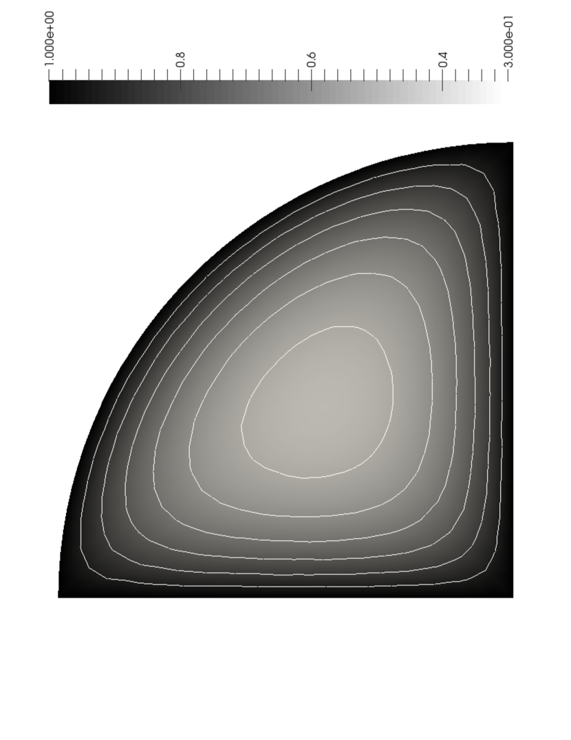
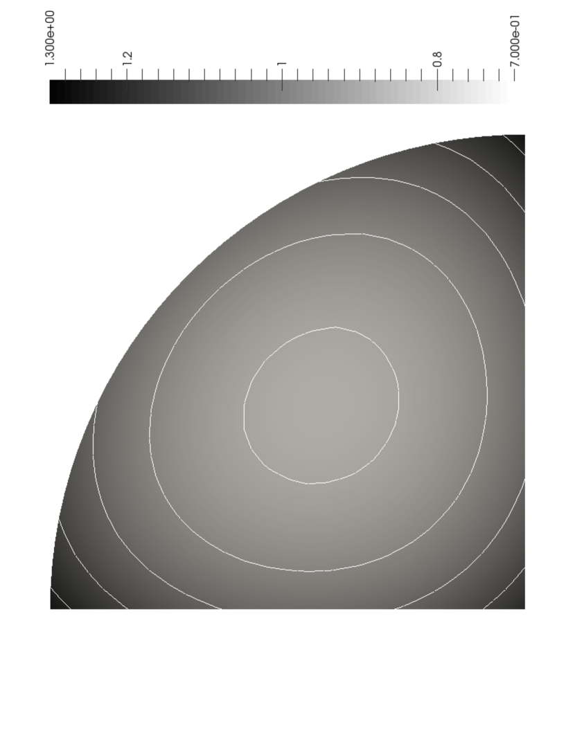
Figure 1. Approximate solutions for $c_{0}=5$ in two limiting cases: (left) $\alpha=0$ (Dirichlet data), $\min w(x)=0.38688$, $\max w(x)=1$ (achieved on $\Gamma$) and (right) $\alpha=1$ (Neumann data), $\min w(x)=0.7741$, $\max w(x)=1.2417$.

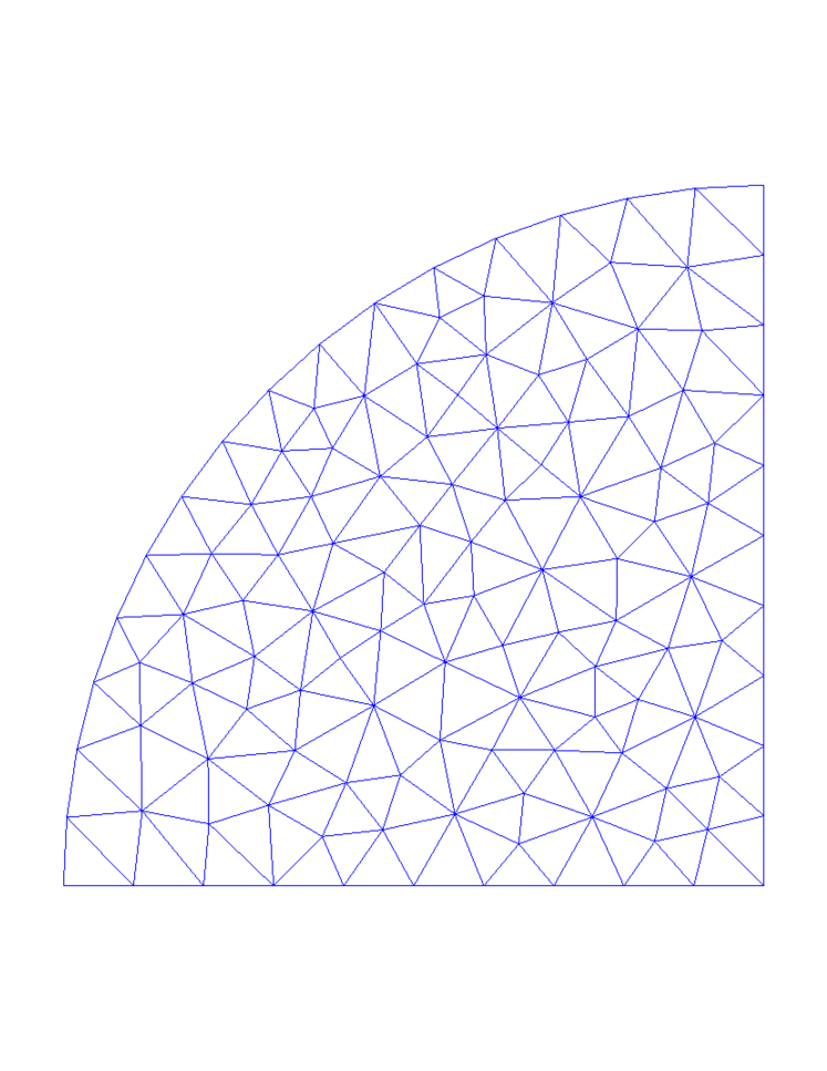
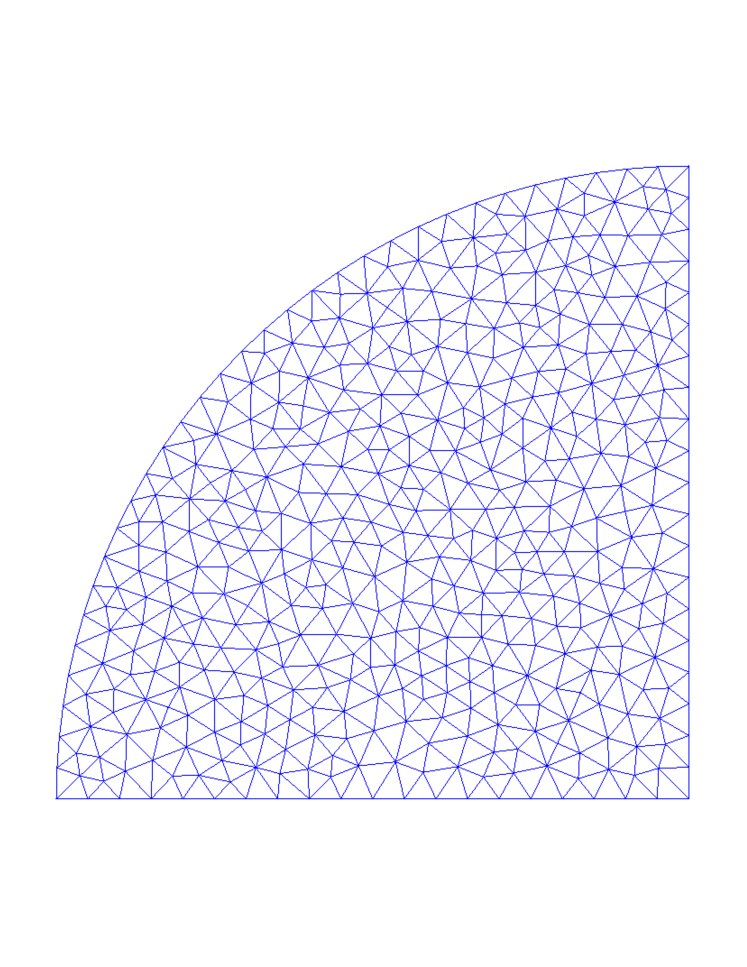
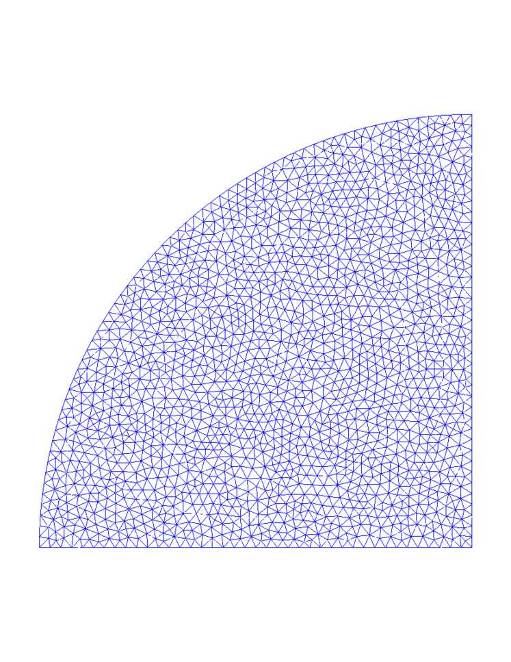
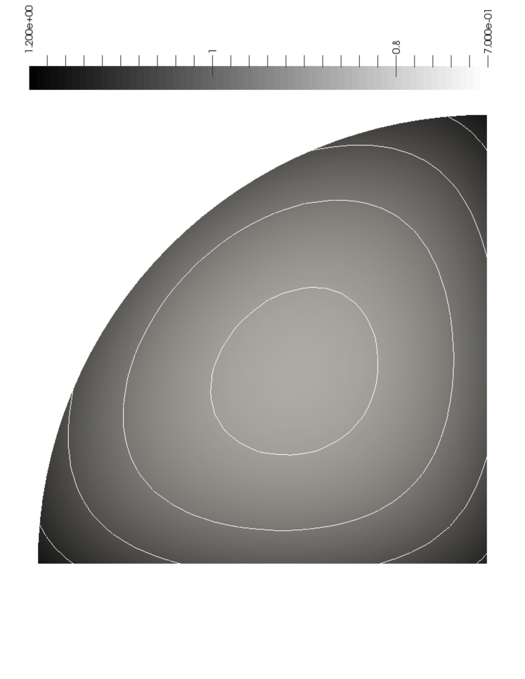
Figure 2. Approximate solutions for $\alpha=0.5$ on three meshes: Left: grid with 123 vertexes and 208 triangles; $\min w(x)=0.7669,\ \max w(x)=1.157$; Middle: grid with 461 vertexes and 848 triangles; $\min w(x)=0.7668,\ \max w(x)=1.151$; Right: grid with 1731 vertexes and 3317 triangles; $\min w(x)=0.7668,\ \max w(x)=1.151$.

On Fig. 1 we show the numerical solution level curves $u(x)=0.9,0.8,0.7,\dots$ for two limiting cases of $\alpha$, namely, the standard elliptic problem with Dirichlet data, $\alpha=0$, and with Neumann data, $\alpha=1$. These two examples are given for comparison with the cases of fractional boundary conditions.

Next, on Fig. 2 we show the computed solution obtained on three different grids for $\alpha=0.5$ and $c_{0}=5$. One can observe a rather weak dependence of the results on the grid size. Note, that in this case the solution is smooth. The solutions of the problem with $\alpha=0.25$ and $\alpha=0.75$ are shown on Fig. 3. The impact of the coefficient $c_{0}$ can be observed on Fig. 4, where we show the approximate solution for $c_{0}=1$ and $c_{0}=25$ that is obtained on a grid with 461 vertexes, a medium size grid.

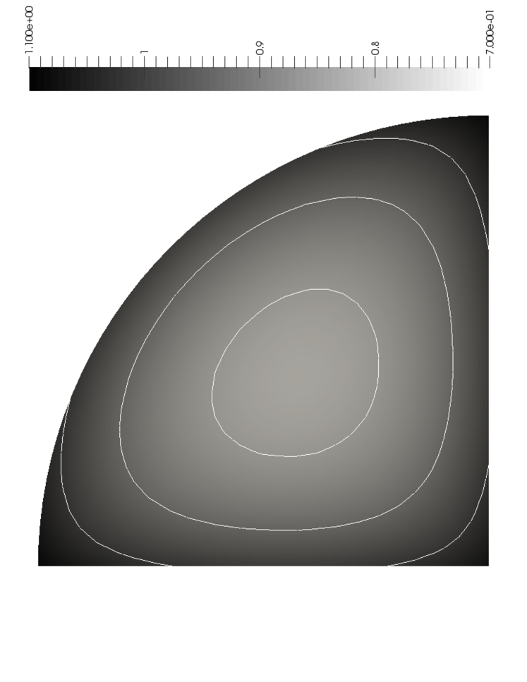
Figure 3. The solution for different $\alpha$: Left: $\alpha=0.25$, $\min w(x)=0.767$, $\max w(x)=1.087$ and Right: $\alpha=0.75$, $\min w(x)=0.769$, $\max w(x)=1.201$.

Figure 4. The solution for different $c_{0}$: Left: $c_{0}=1$, $\min w(x)=2.034$, $\max w(x)=2.246$; Right: $c_{0}=25$ (right), $\min w(x)=0.174$, $\max w(x)=0.690$.

The most important issue concerning the efficiency and the accuracy of a numerical method for solving a boundary value problems for fractional power of elliptic operators or elliptic equations with fractional boundary conditions is the impact of $M$, the number of nodes in the quadrature formula (13) or the number of time steps in (18). Below we report the relative error in $L^{\infty}(\Omega)$ and $L^{2}(\Omega)$-norms:

$$e_{\infty}=\max_{x\in\Omega}|w_{M}(x)-w(x)|/\max_{x\in\Omega}|w(x)|,\quad e_{2}=\|w_{M}(x)-w(x)\|/\|w\|.$$

Here $w_{M}(x)$ is the numerical solution, and $w(x)$ is the reference (practically exact) solution obtained for large $M$, shown in Fig. 2.

The errors, $e_{\infty}$ and $e_{2}$, of the numerical solution of the problem for $c_{0}=5$, $\alpha=0.25,0.5,0.75$ and various $M$ for both methods are shown in Table 1. In these experiments for Method II we take $\delta=0.9$ and $\widetilde{\lambda}_{1}\approx 0.949314$.

First we note that to achieve acceptable accuracy with Method I, we need to use quadrature formulas with a fairly large number of nodes ($M\sim 100$). The highest convergence rates are observed for $\alpha=0.5$. The convergence decreases drastically when $\alpha$ gets close to $0$ or $1$. However, this numerical scheme has asymptotic exponential convergence, see, [4]. Analyzing the numerical data shown on Table 1 we see that: (1) by doubling the quadrature points from $10$ to $20$ the error reduces by a factor of $2$; (2) by doubling the quadrature points from $80$ to $160$ the error reduces by factors of $4$ to $40$ for different $\alpha$. Also, for $\alpha=0.5$ by doubling the quadrature points from $40$ to $80$ the error $e_{2}$ is reduced by a factor of $13$. The same conclusions can be made after analyzing the numerical results of Table 2 as well. This means that an exponential asymptotic convergence rate begins to show for $M$ large enough depending on fractional power $\alpha$.

The numerical results for Method II show, as predicted by the theory, almost second order convergence rate with respect to $\tau$. Note that relatively good accuracy is achieved even for small number of time steps $N$ ($N=M$). From these numerical experiments (performed on smooth solutions) we see that the Method II shows better accuracy for relatively large time-step $\tau$, which translates into fewer computations.

The errors, $e_{\infty}$ and $e_{2}$, of the numerical solution for problems with $\alpha=0.5$ and different values of the coefficient $c_{0}$ are given in Table 2. For Method II we take $\delta=0.2$ and $\widetilde{\lambda}_{1}\approx 0.212867$ at $c_{0}=1$ and $\delta=3$ and $\widetilde{\lambda}_{1}\approx 3.170554$ at $c_{0}=25$. From the numerical experiments we see that these methods are fairly insensitive to the variation of $c_{0}$.

Table 1. Numerical solution error for $c_{0}=5$ and $\alpha=\frac{1}{4},\frac{1}{2},\frac{3}{4}$

		Method I			Method II
$M$	$e$ $\backslash$ $\alpha$	0.25	0.5	0.75	0.25	0.5	0.75
5	$e_{\infty}$	2.5009e-01	1.0492e-01	2.7720e-01	1.4875e-03	1.2809e-03	6.3801e-04
	$e_{2}$	2.6929e-01	1.0819e-01	2.7201e-01	2.1016e-04	2.3152e-04	1.4033e-04
10	$e_{\infty}$	1.5967e-01	4.4602e-02	1.7838e-01	5.3950e-04	4.2429e-04	1.9596e-04
	$e_{2}$	1.7271e-01	4.6029e-02	1.7458e-01	5.6560e-05	6.1306e-05	3.6738e-05
20	$e_{\infty}$	8.4043e-02	1.2636e-02	9.4258e-02	1.8701e-04	1.3399e-04	5.7360e-05
	$e_{2}$	9.1097e-02	1.3043e-02	9.2119e-02	1.4848e-05	1.5628e-05	9.2899e-06
40	$e_{\infty}$	3.3725e-02	2.0501e-03	3.7872e-02	6.1051e-05	4.0353e-05	1.6150e-05
	$e_{2}$	3.6579e-02	2.1162e-03	3.6994e-02	4.0022e-06	3.9635e-06	2.3232e-06
80	$e_{\infty}$	9.2023e-03	1.5283e-04	1.0336e-02	1.8221e-05	1.1398e-05	4.3515e-06
	$e_{2}$	9.9821e-03	1.5781e-04	1.0096e-02	1.0897e-06	1.0015e-06	5.7474e-07
160	$e_{\infty}$	1.4553e-03	3.7728e-06	1.6347e-03	4.9096e-06	2.9878e-06	1.1157e-06
	$e_{2}$	1.5787e-03	3.9520e-06	1.5967e-03	2.8073e-07	2.4428e-07	1.3636e-07

Table 2. Numerical solution error for $\alpha=0.5$ and $c_{0}=1,5,25$

		Method I			Method II
$M$	$e$ $\backslash$ $c_{0}$	1	5	25	1	5	25
5	$e_{\infty}$	1.4067e-01	1.0492e-01	1.1232e-01	1.2847e-03	1.2809e-03	9.4560e-04
	$e_{2}$	1.4056e-01	1.0819e-01	1.3005e-01	3.1276e-04	2.3152e-04	1.2364e-04
10	$e_{\infty}$	6.0161e-02	4.4602e-02	4.7706e-02	5.2113e-04	4.2429e-04	3.0310e-04
	$e_{2}$	6.0112e-02	4.6029e-02	5.5530e-02	1.0988e-04	6.1306e-05	3.3082e-05
20	$e_{\infty}$	1.7066e-02	1.2636e-02	1.3512e-02	1.8893e-04	1.3399e-04	8.9985e-05
	$e_{2}$	1.7052e-02	1.3043e-02	1.5747e-02	3.2926e-05	1.5628e-05	8.8981e-06
40	$e_{\infty}$	2.7691e-03	2.0501e-03	2.1923e-03	6.2310e-05	4.0353e-05	2.4683e-05
	$e_{2}$	2.7669e-03	2.1162e-03	2.5551e-03	8.8335e-06	3.9635e-06	2.3307e-06
80	$e_{\infty}$	2.0637e-04	1.5283e-04	1.6345e-04	1.9396e-05	1.1398e-05	6.3911e-06
	$e_{2}$	2.0634e-04	1.5781e-04	1.9053e-04	2.2445e-06	1.0015e-06	5.7694e-07
160	$e_{\infty}$	5.1206e-06	3.7728e-06	4.0639e-06	5.6936e-06	2.9878e-06	1.5981e-06
	$e_{2}$	5.1713e-06	3.9520e-06	4.7688e-06	5.5463e-07	2.4428e-07	1.2614e-07

References

- [1] L. Aceto and P. Novati, Rational approximation to the fractional Laplacian operator in reaction-diffusion problems. SIAM Journal on Scientific Computing, 39 No 1 (2017), A214–A228.
- [2] M.G. Armentano, The effect of reduced integration in the Steklov eigenvalue problem. Mathematical Modelling and Numerical Analysis, 38 No 1 (2004), 27–36.
- [3] I. Babuska and J. Osborn, Eigenvalue problems. In: Handbook of numerical analysis., 2 (1991) 641-787.
- [4] A. Bonito and J. Pasciak, Numerical approximation of fractional powers of elliptic operators. Mathematics of Computation, 84 No 295 (2015), 2083–2110.
- [5] A. Bueno-Orovio, D. Kay, and K. Burrage, Fourier spectral methods for fractional-in-space reaction-diffusion equations. BIT Numerical Mathematics, 54 No 4 (2014), 1–18.
- [6] K. Burrage, N. Hale, and D. Kay, An efficient implicit FEM scheme for fractional-in-space reaction-diffusion equations. SIAM Journal on Scientific Computing, 34 No 4 (2012), A2145–A2172.
- [7] I. Gavrilyuk, W. Hackbusch, and B. Khoromskij, Data-sparse approximation to the operator-valued functions of elliptic operator. Mathematics of Computation, 73 No 247 (2004), 1297–1324.
- [8] I. Gavrilyuk, W. Hackbusch, and B. Khoromskij, Data-sparse approximation to a class of operator-valued functions. Mathematics of Computation, 74 No 250 (2005), 681–708.
- [9] S. Harizanov, R. Lazarov, P. Marinov, S. Margenov, and Y. Vutov, Optimal Solvers for Linear Systems with Fractional Powers of Sparse SPD Matrices, submitted NLAA, posted as arXiv:1612.04846v1).
- [10] N.J. Higham, Functions of matrices: theory and computation. SIAM, Philadelphia (2008).
- [11] M. Ilić, F. Liu, I. Turner, and V. Anh, Numerical approximation of a fractional-in-space diffusion equation. II. With nonhomogeneous boundary conditions. Fractional Calculus and Applied Analysis, 9 No 4 (2006), 333–349.
- [12] M. Ilić, I.W. Turner, and V. Anh, A numerical solution using an adaptively preconditioned Lanczos method for a class of linear systems related with the fractional Poisson equation. International Journal of Stochastic Analysis, (2008), 1–26, Article ID 104525.
- [13] A.A. Kilbas, H.M. Srivastava, and J.J. Trujillo, Theory and Applications of Fractional Differential Equations. North-Holland mathematics studies. Elsevier, Amsterdam (2006).
- [14] M.A. Krasnoselskii, P.P. Zabreiko, E.I. Pustylnik, and P.E. Sobolevskii, Integral Operators in Spaces of Summable Functions. Noordhoff International Publishing (1976).
- [15] R. Metzler, J.H. Jeon, A.G. Cherstvy, and E. Barkai, Anomalous diffusion models and their properties: non-stationarity, non-ergodicity, and ageing at the centenary of single particle tracking. Physical Chemistry Chemical Physics, 16 No 44 (2014), 24128–24164.
- [16] I. Podlubny, Fractional differential equations: an introduction to fractional derivatives, fractional differential equations, to methods of their solution and some of their applications, v. 198, Academic press (1998).
- [17] A.A. Samarskii, The theory of difference schemes. Marcel Dekker, New York (2001).
- [18] V. Thomée, Galerkin Finite Element Methods for Parabolic Problems. Springer Series in Computational Mathematics. Springer (2006).
- [19] P.N. Vabishchevich, Numerically solving an equation for fractional powers of elliptic operators. Journal of Computational Physics, 282 No 1 (2015), 289–302.