Optical parallel computation similar to quantum computation based on optical fields modulated with pseudorandom phase sequences

Abstract

We propose an optical parallel computation similar to quantum computation that can be realized by introducing pseudorandom phase sequences into classical optical fields with two orthogonal modes. Based on the pseudorandom phase sequences, we first propose a theoretical framework of “phase ensemble model” referring from the concept of quantum ensemble. Using the ensemble model, we further demonstrate the inseparability of the fields similar to quantum entanglement. It is interesting that a $N2^{N}$ dimensional Hilbert space spanned by $N$ optical fields is larger than that spanned by $N$ quantum particles. This leads a problem for our scheme that is not the lack of resources but the redundancy of resources. In order to reduce the redundancy, we propose a special sequence permutation mechanism to efficiently imitate certain quantum states, including the product state, Bell states, GHZ state and W state. For better fault tolerance, we further devise each orthogonal mode of optical fields is measured to assign discrete values. Finally, we propose a generalized gate array model to imitate some quantum algorithms, such as Shor’s algorithm, Grover’s algorithm and quantum Fourier algorithm. The research on the optical parallel computation might be important, for it not only has the potential beyond quantum computation, but also provides useful insights into fundamental concepts of quantum mechanics.

LABEL:FirstPage1

Introduction

It has been widely known that quantum computation enormously promotes computational efficiency by using several basic and purely physical features of quantum mechanics, such as coherent superposition, quantum entanglement, measurement collapse etc. Nielsen . The accelerant ability of quantum computation is related to quantum entanglement and tensor product structure, which are essential to allow growing exponentially the computation resource with the number of qubits Jozsa ; Braunstein . Yet the practical quantum computations are difficult to be realized for restrictions of quantum system controllability, decoherence property and measurement randomness Knill ; Nielsen2 ; Browne ; Kok .

The classical simulation of quantum systems, especially of quantum entanglement has been under investigation for a long time Cerf ; Massar ; Spreeuw . In addition to easy implementations, the researches on the classical simulations can help understand some fundamental concepts in quantum mechanics. However, it has been pointed out by several researchers that the classical simulation of quantum systems requires exponentially scaling of physical resources with the number of quantum particles Jozsa ; Spreeuw . In Ref. Spreeuw , an optical analogy to quantum systems was introduced, in which the number of light beams and optical components required grows exponentially with the number of qubits. In Ref. Vidal , a classical protocol to efficiently simulate any pure-state quantum computation is presented, yet the amount of entanglement involved is restricted. In Ref. Jozsa , it is elucidated that in classical theory, the state space of a composite system is the direct product of subsystems, whereas in quantum theory it is the tensor product. It is generally accepted that the essential distinction between direct and tensor products is precise the phenomenon of quantum entanglement, and regarded as the origin of the limitation of any classical systems. Recently, several researches have proposed a new concept of realization of classical entanglement based on classical optical fields by introducing a new degree of freedom, such as orbital angular momentum, to realize tensor product in quantum entanglement Toppel . However, the method cannot provide enough orthogonal degrees of freedom, which the scalability might be doubtful.

In this paper, we propose an optical parallel computation similar to quantum computation that can be realized by introducing pseudorandom phase sequences into optical fields with two orthogonal modes Fu1 . The two orthogonal modes (polarization or transverse) of optical field are encoded as optical analogies to quantum bits $\left|0\right\rangle$ and $\left|1\right\rangle$ Fu ; dragoman ; Lee . In wireless and optical communications, orthogonal pseudorandom sequences have been widely applied to Code Division Multiple Access (CDMA) communication technology as a way to distinguish different users Golomb ; Viterbi ; Peterson . A set of pseudorandom sequences guided by a Galois field GF($p$) is generated by using a linear feedback shift register method, which satisfies orthogonal, closure and balance properties Golomb ; Viterbi ; Peterson . In Phase Shift Keying (PSK) communication technology PSK , the information is encoded in the phase of classical optical/electromagnetic fields, where the phase values in $\left\{0,2\pi/p,\cdots,2\pi\left(p-1\right)/p\right\}$ for the $p$-ary communication. Combining the two communication technologies, we introduce the pseudorandom phase sequences in our scheme. Guaranteed by the orthogonal property, the optical/electromagnetic fields modulated with different pseudorandom phase sequences can transmit in one communication channel simultaneously without crosstalk, and can be easily distinguished by implementing a coherent demodulation Viterbi .

Different from other schemes Spreeuw ; Toppel , the pseudorandom phase sequences employed in our scheme are able to provide not only scalable degrees of freedom to support arbitrary dimensional tensor product structure, also a theoretical framework of “phase ensemble model” similar to the concept of quantum ensemble. Using the ensemble model, we can demonstrate the inseparable correlation between the optical fields with different pseudorandom phase sequences similar to quantum entanglement. It is interesting that a $N2^{N}$ dimensional Hilbert space can be spanned by $N$ optical fields which is larger than that spanned by $N$ quantum particles. This leads a problem for our scheme that is not the lack of resources but the redundancy of resources. In order to reduce the redundancy, we have to introduce a sequential cycle permutation mechanism based on coherent demodulation to realize the bijection imitation of certain quantum states. Optical analogies to some typical quantum states are also discussed, including Bell states, GHZ and W states. For better fault tolerance, we devise each orthogonal mode of optical fields is measured to assign discrete values. It means that a discrete computation model is provided in our scheme. Furthermore, we propose a gate array model to imitate quantum computation based on four kinds of mode control gates. As some examples, we demonstrate the imitations of Shor’s algorithm Shor , Grover’s algorithm Grover and quantum Fourier algorithm Nielsen . In order to verify the feasibility, we numerically simulate our scheme using the widely used optical communication simulation software OPTISYSTEM.

The paper is organized as follows: In Section I, we introduce some preparing knowledges required later in this paper. In Section II, a theoretical framework of “phase ensemble model” and the optical analogies of several typical quantum states are then discussed. In Section III, a gate array model to imitate quantum computation is proposed. Finally, we summarize our conclusions in Section IV.

I Preparing knowledges

In this section, we introduce some notations and basic results required later in this paper. We first introduce pseudorandom phase sequences (PPSs) and their properties. Then we introduce the scheme of modulation and demodulation on optical fields with PPSs. Finally, we discuss the similarities between an optical field and a single-particle quantum state.

I.1 Pseudorandom phase sequences and their properties

As far as we know, orthogonal pseudorandom sequences have been widely applied to CDMA communication technology as a way to distinguish different users Golomb ; Viterbi ; Peterson . A set of pseudorandom sequences is generated from a shift register guided by a Galois field GF($p$), which satisfies orthogonal, closure and balance properties. The orthogonal property ensures that sequences of the set are independent and distinguished each other with an excellent correlation property. The closure property ensures that any linear combination of the sequences remains in the same set. The balance property ensures that the occurrence rate of all non-zero-element in every sequence is equal, and the the number of zero-elements is exactly one less than the other elements. One famous generator of pseudorandom sequences is linear feedback shift register (LFSR), which can produce a maximal period sequence, called m-sequence Golomb . We consider an m-sequence of period $N-1$ ($N=p^{s}$) generated by a primitive polynomial of degree $s$ over GF($p$). Since the correlation between different shifts of an m-sequence is almost zero, they can be used as different codes with their excellent correlation property. In this regard, the set of $N-1$ m-sequences of length $N-1$ can be obtained by cyclic shifting of a single m-sequence.

In this paper, we employ PPSs with $2$-ary $\{0,\pi/2\}$ phase shift modulation. Although the phases should uniformly distribute in $\left[0,2\pi\right]$, the $2$-ary PSK is the most frequently used modulation due to the phase symmetry in practical communication systems PSK . We first propose a scheme to generate a PPS set $\Xi=\left\{\lambda^{\left(1\right)},\lambda^{\left(2\right)},\ldots,\lambda^{\left(N\right)}\right\}$ over GF($2$). $\lambda^{\left(N\right)}$ is an all-zero sequence and other sequences can be generated by using the method as follows:

(1) given a primitive polynomial of degree $s$ over GF($2$), a base sequence of a length $2^{s}-1$ is generated by using LFSR;

(2) other sequences are obtained by cyclic shifting of the base sequence;

(3) by adding a zero-element to the end of each sequence, the occurrence rates of all elements in all sequences are equal with each other;

(4) mapping the elements of the sequences to $\{0,\pi/2\}$: $0$ mapping $0$, $1$ mapping $\pi/2$.

In Fig. 1, we demonstrate the relationship between time slots, an m-sequence and phase sequence $\lambda^{\left(i\right)}$ with $N$ phase units $\lambda^{\left(i\right)}=\left[\begin{array}[]{cccc}\lambda_{1}^{\left(i\right)}&\lambda_{2}^{\left(i\right)}&...&\lambda_{N}^{\left(i\right)}\end{array}\right]$. For better understanding our scheme, the PPSs in the cases of modulating $4$ and $8$ optical fields are illustrated below. An m-sequence of length $2^{2}-1$ is generated by a primitive polynomial of the lowest degree over $GF(2)$, which is $\left[\begin{array}[]{ccc}1&0&1\end{array}\right]$. Then we obtain the set $\Xi$ that includes $4$ PPSs of length $4$: $\left\{\lambda^{\left(1\right)},\lambda^{\left(2\right)},\lambda^{\left(3\right)},\lambda^{\left(4\right)}\right\}$, where $\lambda^{\left(4\right)}$ is the all-zero sequence. The PPSs can be used to modulate up to $4$ optical fields as follows

$$\lambda^{\left(1\right)} = \left[\begin{array}[]{cccc}1&0&1&0\end{array}\right]\times\pi/2,$$ (2)

$$\lambda^{\left(2\right)} = \left[\begin{array}[]{cccc}1&1&0&0\end{array}\right]\times\pi/2,$$ (4)

$$\lambda^{\left(3\right)} = \left[\begin{array}[]{cccc}0&1&1&0\end{array}\right]\times\pi/2,$$ (6)

$$\lambda^{\left(4\right)} = \left[\begin{array}[]{cccc}0&0&0&0\end{array}\right]\times\pi/2.$$ (8)

By using the same method, an m-sequence of length $2^{3}-1$ is generated by a primitive polynomial of the $2^{nd}$ lowest degree over $GF(2)$, which is $\left[\begin{array}[]{ccccccc}1&0&0&1&0&1&1\end{array}\right]$. Then we obtain the set $\Xi$ that includes $8$ PPSs of length $8$: $\left\{\lambda^{\left(1\right)},\lambda^{\left(2\right)}\ldots,\lambda^{\left(8\right)}\right\}$, where the PPSs are shown as follows

$$\lambda^{\left(1\right)} = \left[\begin{array}[]{cccccccc}1&0&0&1&0&1&1&0\end{array}\right]\times\pi/2,$$ (10)

$$\lambda^{\left(2\right)} = \left[\begin{array}[]{cccccccc}1&1&0&0&1&0&1&0\end{array}\right]\times\pi/2,$$ (12)

$$\lambda^{\left(3\right)} = \left[\begin{array}[]{cccccccc}1&1&1&0&0&1&0&0\end{array}\right]\times\pi/2,$$ (14)

$$\lambda^{\left(4\right)} = \left[\begin{array}[]{cccccccc}0&1&1&1&0&0&1&0\end{array}\right]\times\pi/2,$$ (16)

$$\lambda^{\left(5\right)} = \left[\begin{array}[]{cccccccc}1&0&1&1&1&0&0&0\end{array}\right]\times\pi/2,$$ (18)

$$\lambda^{\left(6\right)} = \left[\begin{array}[]{cccccccc}0&1&0&1&1&1&0&0\end{array}\right]\times\pi/2,$$ (20)

$$\lambda^{\left(7\right)} = \left[\begin{array}[]{cccccccc}0&0&1&0&1&1&1&0\end{array}\right]\times\pi/2,$$ (22)

$$\lambda^{\left(8\right)} = \left[\begin{array}[]{cccccccc}0&0&0&0&0&0&0&0\end{array}\right]\times\pi/2.$$ (24)

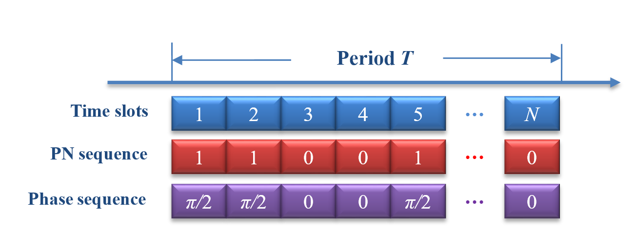
Figure 1: The relationship between time slots, an m-sequence and PPS is shown.

Further, we define a map $f:\lambda\rightarrow e^{i\lambda}$ on the set of $\Xi$, and obtain a new sequence set $\Omega=\left\{\varphi^{\left(j\right)}\left|\varphi^{\left(j\right)}=e^{i\lambda^{\left(j\right)}},\right.j=1,\ldots,N\right\}$. The map $f$ corresponds to the phase modulations of the PPSs on optical fields. According to the properties of m-sequence, we can obtain following properties of the set $\Omega$, (1) the closure property: the product of any sequences remains in the same set, in additional $\pi$ phase contributed by the power of a sequence; (2) the balance property: in exception to $\varphi^{\left(N\right)}$, any sequences of the set $\Omega$ satisfy,

$$\sum\limits_{k=1}^{N}e^{i\theta}\varphi_{k}^{\left(j\right)}=\sum\limits_{k=1}^{N}e^{i\left(\lambda_{k}^{\left(j\right)}+\theta\right)}=0,\forall\theta\in\mathbb{R};$$ (25)

(3) the orthogonal property: any two sequences satisfy the following normalized correlation

$$E\left({\varphi^{\left(i\right)},\varphi^{\left(j\right)}}\right) = \frac{1}{N}\sum\limits_{k=1}^{N}{\varphi_{k}^{\left(i\right)}\varphi_{k}^{\left(j\right)\ast}}$$ (26)

$$= \left\{\begin{array}[]{cc}1,&i=j\\ 0,&i\neq j\end{array}\right..$$ (29)

In conclusion, according to the properties above, the optical fields modulated with different PPSs become independent and distinguishable in any case.

I.2 Modulation and demodulation on optical fields with pseudorandom phase sequences

In this section, we mainly focus on the modulation and demodulation of optical fields with single polarization mode. We first consider the modulation process of an optical field with a PPS $\lambda^{\left(i\right)}$ from the set $\Xi$. For example, we choose $\lambda^{\left(1\right)}$ to modulate the optical field labeled as the signal optical (SO) field, its electric field component is

$$E_{S}\left(t\right)=A_{S}e^{-i\left(\omega t+\lambda_{k}^{\left(1\right)}\right)},$$ (30)

where $A_{S},\omega$ are the amplitude and frequency of the optical field respectively, and $\lambda_{k}^{\left(1\right)}$ is the phase unit of $\lambda^{\left(1\right)}$ at the $k$-th time slot.

In order to perform the demodulation of PPS, we design a coherent detection scheme as shown in Fig. 2 that has been widely used in the coherent communication Viterbi . In the detection scheme, the local optical (LO) beam and the SO beam interfere with each other through a beam coupler (BC). In order to ensure the coherence of them, the two beams can be split from the same optical source through a beam splitter (BS). The LO field can be expressed as

$$E_{L}\left(t\right)=A_{L}e^{-i\left(\omega t+\lambda_{k}^{\left(n\right)}\right)},$$ (31)

where $\lambda^{\left(n\right)}$ can be an arbitrary sequence of the set $\Xi$ and the amplitude $A_{L}=A_{S}$ assumed. After the coherent superposition through the BC, the output fields can be expressed as

$$\left(\begin{array}[]{c}E_{1}\left(t\right)\\ E_{2}\left(t\right)\end{array}\right)=\frac{1}{\sqrt{2}}\left(\begin{array}[]{cc}1&i\\ -i&1\end{array}\right)\left(\begin{array}[]{c}E_{S}\left(t\right)\\ E_{L}\left(t\right)\end{array}\right)=\frac{A_{S}}{\sqrt{2}}\left(\begin{array}[]{c}e^{-i\left(\omega t+\lambda_{k}^{\left(1\right)}\right)}+ie^{-i\left(\omega t+\lambda_{k}^{\left(n\right)}\right)}\\ -ie^{-i\left(\omega t+\lambda_{k}^{\left(1\right)}\right)}+e^{-i\left(\omega t+\lambda_{k}^{\left(n\right)}\right)}\end{array}\right).$$ (32)

Then, the output electric signals of photodetectors $D_{1}$ and $D_{2}$ is proportional to

$$D_{1} = \mu\left|E_{1}\left(t\right)\right|^{2}=\mu\left|A_{S}\right|^{2}\left[1-\sin\left(\lambda_{k}^{\left(1\right)}-\lambda_{k}^{\left(n\right)}\right)\right],$$ (33)

$$D_{2} = \mu\left|E_{2}\left(t\right)\right|^{2}=\mu\left|A_{S}\right|^{2}\left[1+\sin\left(\lambda_{k}^{\left(1\right)}-\lambda_{k}^{\left(n\right)}\right)\right],$$

where $\mu$ is the parameter related to the sensitivity of photodetectors. Finally, after correlation analysis of the two electric signals, we can obtain as follow

$$E=\left\langle D_{1}D_{2}\right\rangle=\frac{\mu^{2}\left|A_{S}\right|^{4}\Delta T}{2}\sum\limits_{k=1}^{8}\left[1+\cos 2\left(\lambda_{k}^{\left(1\right)}-\lambda_{k}^{\left(n\right)}\right)\right]=\left\{\begin{array}[]{c}8\mu^{2}\left|A_{S}\right|^{4}\Delta T,\ n=1\\ 4\mu^{2}\left|A_{S}\right|^{4}\Delta T,\ n\neq 1\end{array}\right.,$$ (34)

where $\Delta T$ is the PPS time slot. In addition to a constant, the result satisfies the orthogonality of PPS.

To verify the above scheme, we utilize the software OPTISYSTEM to numerically simulate it. Fig. 3 shows the electric signals of two photodetectors within a sequence period. Fig. 4 shows the correlation analysis results of the SO field and the LO field modulated with different PPSs. We can find out the correlation result is the largest when the SO and LO fields modulated with the same PPS. Hence, the orthogonality of PPSs can be used to distinguish the optical fields with different PPSs.

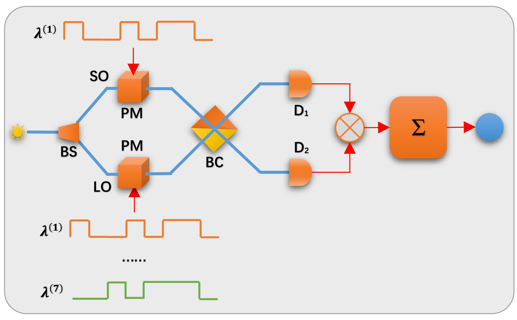
Figure 2: The scheme of the coherent detection of pseudorandom phase sequence is shown, where SO: signal optical field, LO: local optical field, BS: beam splitter, PM: phase modulators, BC: beam coupler, $D_{1}$ and $D_{2}$: photodetectors, $\otimes$: multiplier and $\Sigma$: integrator (integrate over entire sequence period).

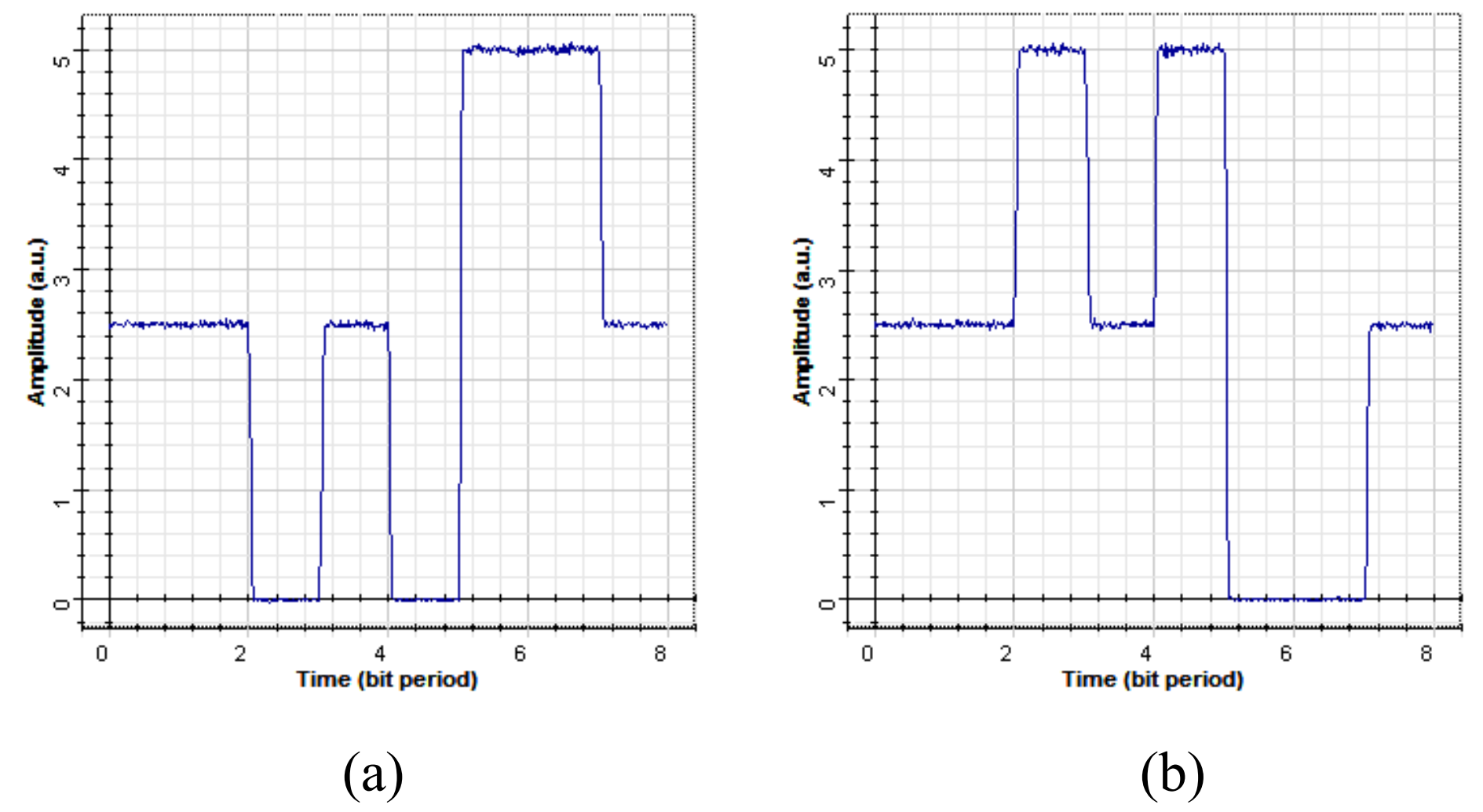
Figure 3: The electric signals of $D_{1}$(a) and $D_{2}$(b) are shown when the sequence of the LO field is $\lambda^{\left(5\right)}$.

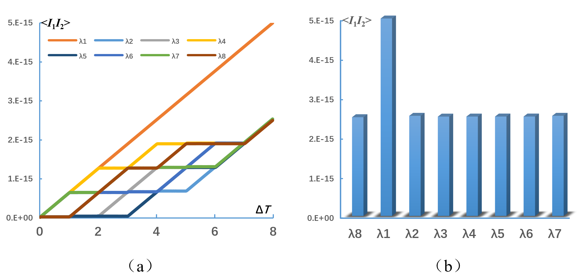
Figure 4: The correlation analysis results are shown when the SO field with $\lambda^{\left(1\right)}$ and the LO fields with $\lambda^{\left(1\right)}\sim\lambda^{\left(8\right)}$ (corresponding to $\lambda 1\sim\lambda 8$), where (a) is the correlation intergrals vary with the sequence time slots $\Delta T$, and (b) is the final correlation results.

I.3 Similarities between an optical field and a single-particle quantum state

We note the similarities between Maxwell equation and Schrödinger equation Fu . In fact, some properties utilized in quantum information are wave properties, where the wave might not be a quantum wave Spreeuw . Analogously to quantum states, optical fields also obey a superposition principle, and can be transformed to any superposition state by unitary transformations. Those analogous properties make possible the analogies to quantum states using polarization or transverse modes of optical fields Spreeuw ; Fu ; dragoman ; Lee .

We first consider two orthogonal modes (polarization or transverse) of optical fields, as the optical analogies to quantum bits (qubits) $\left|0\right\rangle$ and $\left|1\right\rangle$

$$\left|0\right\rangle=\left(\begin{array}[]{c}1\\ 0\end{array}\right),\left|1\right\rangle=\left(\begin{array}[]{c}0\\ 1\end{array}\right).$$ (35)

Thus, any quantum state of a single particle can be imitated by the mode superposition of optical field as follow

$$\left|\psi\right\rangle=\alpha\left|0\right\rangle+\beta\left|1\right\rangle,$$ (36)

where $\left|\alpha\right|^{2}+\left|\beta\right|^{2}=1,\left(\alpha,\beta\in\mathbb{C}\right)$. Obviously, all the mode superposition can also span a Hilbert space. We can transform a mode state to any other state using the unitary transformation as follow Nielsen

$$\hat{U}\left(\alpha,\beta,\gamma,\delta\right)=e^{i\alpha}\left(\begin{array}[]{cc}e^{-i\beta/2}&0\\ 0&e^{i\beta/2}\end{array}\right)\left(\begin{array}[]{cc}\cos\frac{\gamma}{2}&-\sin\frac{\gamma}{2}\\ \sin\frac{\gamma}{2}&\cos\frac{\gamma}{2}\end{array}\right)\left(\begin{array}[]{cc}e^{-i\delta/2}&0\\ 0&e^{i\delta/2}\end{array}\right),$$ (37)

where $\alpha,\beta,\gamma,\delta$ are real-valued. The modes $\left|0\right\rangle$ and $\left|1\right\rangle$ can be transformed to any mode superpositions by using $\hat{U}\left(\alpha,\beta,\gamma,\delta\right)$, respectively, as follows

$$\hat{U}\left(\alpha,\beta,\gamma,\delta\right)\left|0\right\rangle = e^{i\left(\alpha-\delta/2\right)}\left(e^{-i\beta/2}\cos\frac{\gamma}{2}\left|0\right\rangle+e^{i\beta/2}\sin\frac{\gamma}{2}\left|1\right\rangle\right),$$ (38)

$$\hat{U}\left(\alpha,\beta,\gamma,\delta\right)\left|1\right\rangle = e^{i\left(\alpha+\delta/2\right)}\left(-e^{-i\beta/2}\sin\frac{\gamma}{2}\left|0\right\rangle+e^{i\beta/2}\cos\frac{\gamma}{2}\left|1\right\rangle\right).$$

Now, we consider some optical devices with one input and two outputs, such as a beam splitter or a mode splitter, which split one input field $\left|\psi_{in}\right\rangle=\alpha\left|0\right\rangle+\beta\left|1\right\rangle$ into two output fields $\left|\psi_{out}^{\left(a\right)}\right\rangle$ and $\left|\psi_{out}^{\left(b\right)}\right\rangle$. For the case of the beam splitter, the output fields are $\left|\psi_{out}^{\left(a\right)}\right\rangle=C_{a}\left(\alpha\left|0\right\rangle+\beta e^{i\phi_{a}}\left|1\right\rangle\right)$ and $\left|\psi_{out}^{\left(b\right)}\right\rangle=C_{b}\left(\alpha\left|0\right\rangle+\beta e^{i\phi_{b}}\left|1\right\rangle\right)$ with an arbitrary power ratio $\left|C_{a}\right|^{2}:\left|C_{b}\right|^{2}$ between the output beams, where $\phi_{a,b}$ are the additional phases due to the splitter. For the case of the mode splitter, the output fields are $\left|\psi_{out}^{\left(a\right)}\right\rangle=\alpha e^{i\phi_{a}}\left|0\right\rangle$ and $\left|\psi_{out}^{\left(b\right)}\right\rangle=\beta e^{i\phi_{b}}\left|1\right\rangle$, where $\phi_{a,b}$ are also the additional phases. Conversely, the devices can act as a beam coupler or a mode coupler in which beams or modes from two inputs are combined into the one output.

II Optical analogies to multiparticle quantum states

In this section, we discuss optical analogies to multiparticle quantum states using optical fields modulated with PPSs. We first demonstrate that $N$ optical fields modulated with $N$ different PPSs can span a $N2^{N}$ dimensional Hilbert space that contains a tensor product structure Fu1 . Then, we introduce a phase ensemble model to imitate the quantum ensemble. Further, by performing coherent demodulation scheme, we can obtain a mode status matrix of the optical fields. Based on the mode status matrix, we propose a sequential cycle permutation mechanism (SCPM) to imitate some typical quantum states, such as the product state, Bell states, GHZ state and W state.

II.1 Ensemble model labeled by pseudorandom phase sequences

In Fu1 , an effective simulation of quantum entanglement using optical fields modulated with PPSs was discussed. In this paper, we will promote this proposal further.

Referring from the concept of quantum ensemble, we propose a new concept of a pseudorandom phase ensemble model. A phase ensemble is defined as a large number of same optical fields modulated with different PPSs $\lambda^{(i)}$, which are labeled by the phase units $\theta_{k}$ of $\lambda^{(i)}$. A phase ensemble is discrete if the phase unit $\theta_{k}$ is a uniformly distributed discrete value within $[0,2\pi]$. Then we can define that a phase ensemble is complete if finite phase units are ergodic. According to m-sequence theory, the occurrence of each value in a sequence is the same. The phase ensemble is obviously ergodic in finite length. Clearly, we can conclude that optical fields modulated with PPSs constitute a complete discrete phase ensemble.

An ensemble average is defined as weighted average of any sequence $A^{(i)}$ within a sequence period as follow

$$\bar{A}=\frac{1}{N}\sum\limits_{k=1}^{N}A^{(i)}=\frac{1}{N}\sum\limits_{k=1}^{N}A_{k}^{(i)},$$ (39)

where $A_{k}^{(i)}$ is a sequence unit labled by the phase unit $\theta_{k}$. A normalized correlation for two sequences $A^{(i)}$ and $A^{(j)}$ is defined as

$$E\left(A^{(i)},A^{(j)}\right)=\frac{1}{N}\sum\limits_{k=1}^{N}A_{k}^{(i)}A_{k}^{(j)\ast},$$ (40)

where $A_{k}^{(i)},A_{k}^{(j)}$ are the sequence units of $A^{(i)},A^{(j)}$ labled by the phase unit $\theta_{k}$, respectively.

II.1.1 Hilbert space of basis states in the phase ensemble model

Now we discuss a Hilbert space spanned by optical fields modulated with PPSs. There are two orthogonal modes (polarization or transverse) of the optical field, which are denoted by $\left|0\right\rangle$ and $\left|1\right\rangle$, respectively. Thus, a qubit state $\left|\psi\right\rangle=\alpha\left|0\right\rangle+\beta\left|1\right\rangle$ can be expressed by the mode superposition, where $|\alpha|^{2}+|\beta|^{2}=1,(\alpha,\beta\in C)$. Obviously, each mode superposition can span a two  dimensional Hilbert space. Choosing any $N$ PPSs from the set $\Xi$ to modulate $N$ optical fields, we can obtain the states expressed as follows

$$\begin{array}[]{c}\left|\psi_{1}\right\rangle=e^{i\lambda^{(1)}}\left(\alpha_{1}\left|0\right\rangle+\beta_{1}\left|1\right\rangle\right),\\ \vdots\\ \left|\psi_{N}\right\rangle=e^{i\lambda^{(N)}}\left(\alpha_{N}\left|0\right\rangle+\beta_{N}\left|1\right\rangle\right).\end{array}$$ (41)

According to the properties of PPSs and Hilbert space, we can define the inner product of any two fields $\left|\psi_{a}\right\rangle$ and $\left|\psi_{b}\right\rangle$. We obtain the orthogonal property as follow

$$\left\langle\psi_{a}|\psi_{b}\right\rangle=\frac{1}{N}\sum\limits_{k=1}^{N}e^{i(\lambda_{k}^{(b)}-\lambda_{k}^{(a)})}(\alpha_{a}^{\ast}\alpha_{b}+\beta_{a}^{\ast}\beta_{b})=\left\{\begin{array}[]{c}1,a=b,\\ 0,a\neq b,\end{array}\right.$$ (42)

where $\lambda_{k}^{(a)},\lambda_{k}^{(b)}$ are the $k$-th units of $\lambda^{(a)}$ and $\lambda^{(b)}$, respectively. The orthogonal property supports the tensor product structure of the multiple fields Fu1 .

A formal product state $\left|\Psi\right\rangle$ for the $N$ optical fields is defined as being a direct product of $\left|\psi_{n}\right\rangle$,

$$\left|\Psi\right\rangle\equiv\left|\psi_{1}\right\rangle\otimes\left|\psi_{2}\right\rangle\otimes\cdots\otimes\left|\psi_{N}\right\rangle.$$ (43)

According to the definition, $N$ optical fields of Eq. (41) can be expressed as the following state

$$\left|\Psi\right\rangle=e^{i\lambda^{S}}\left(\alpha_{1}\left|0\right\rangle+\beta_{1}\left|1\right\rangle\right)\otimes\left(\alpha_{2}\left|0\right\rangle+\beta_{2}\left|1\right\rangle\right)\otimes\cdots\otimes\left(\alpha_{N}\left|0\right\rangle+\beta_{N}\left|1\right\rangle\right),$$ (44)

where $\lambda^{S}=\sum\nolimits_{n=1}^{N}\lambda^{\left(n\right)}$. By using an array of several mode transformation gates, the optical field $\left|\psi_{n}\right\rangle$ can be transformed from Eq. (41) to the following general state

$$\left|\psi_{n}\right\rangle=\sum\limits_{i=1}^{N}\alpha_{n}^{\left(i\right)}e^{i\lambda^{\left(i\right)}}\left|0\right\rangle+\sum\limits_{j=1}^{N}\beta_{n}^{\left(j\right)}e^{i\lambda^{\left(j\right)}}\left|1\right\rangle.$$ (45)

Then, the formal product state $\left|\Psi\right\rangle$ can be written as

$$\left|\Psi\right\rangle=\left(\sum\limits_{i=1}^{N}\alpha_{1}^{\left(i\right)}e^{i\lambda^{\left(i\right)}}\left|0\right\rangle+\sum\limits_{j=1}^{N}\beta_{1}^{\left(j\right)}e^{i\lambda^{\left(j\right)}}\left|1\right\rangle\right)\otimes\cdots\otimes\left(\sum\limits_{i=1}^{N}\alpha_{N}^{\left(i\right)}e^{i\lambda^{\left(i\right)}}\left|0\right\rangle+\sum\limits_{j=1}^{N}\beta_{N}^{\left(j\right)}e^{i\lambda^{\left(j\right)}}\left|1\right\rangle\right).$$ (46)

Further, we can obtain each item of the superposition of $\left|\Psi\right\rangle$ as follows

$$\begin{array}[]{c}C_{00\cdots 0}\left|00\cdots 0\right\rangle=\left[\left(\sum\limits_{i=1}^{N}\alpha_{1}^{\left(i\right)}e^{i\lambda^{\left(i\right)}}\right)\left(\sum\limits_{i=1}^{N}\alpha_{2}^{\left(i\right)}e^{i\lambda^{\left(i\right)}}\right)\cdots\left(\sum\limits_{i=1}^{N}\alpha_{N}^{\left(i\right)}e^{i\lambda^{\left(i\right)}}\right)\right]\left|00\cdots 0\right\rangle,\\ C_{00\cdots 1}\left|00\cdots 1\right\rangle=\left[\left(\sum\limits_{i=1}^{N}\alpha_{1}^{\left(i\right)}e^{i\lambda^{\left(i\right)}}\right)\left(\sum\limits_{i=1}^{N}\alpha_{2}^{\left(i\right)}e^{i\lambda^{\left(i\right)}}\right)\cdots\left(\sum\limits_{j=1}^{N}\beta_{N}^{\left(j\right)}e^{i\lambda^{\left(j\right)}}\right)\right]\left|00\cdots 1\right\rangle,\\ \vdots\\ C_{11\cdots 1}\left|11\cdots 1\right\rangle=\left[\left(\sum\limits_{j=1}^{N}\beta_{1}^{\left(j\right)}e^{i\lambda^{\left(j\right)}}\right)\left(\sum\limits_{j=1}^{N}\beta_{2}^{\left(j\right)}e^{i\lambda^{\left(i\right)}}\right)\cdots\left(\sum\limits_{j=1}^{N}\beta_{N}^{\left(j\right)}e^{i\lambda^{\left(j\right)}}\right)\right]\left|11\cdots 1\right\rangle,\end{array}$$ (47)

where $\left|i_{1}\ldots i_{N}\right\rangle\equiv\left|i_{1}\right\rangle\otimes\ldots\otimes\left|i_{N}\right\rangle,\left(i_{n}=0\ or\ 1\right)$. According to the closure property, the PPSs of $C_{i_{1}i_{2}\cdots i_{N}}$ remain in the set $\Xi$, which means $C_{i_{1}i_{2}\cdots i_{N}}=\sum\limits_{j=1}^{N}C_{i_{1}i_{2}\cdots i_{N}}^{\left(j\right)}e^{i\lambda^{\left(j\right)}}$. Therefore, we obtain the following conclusion that the formal product state $\left|\Psi\right\rangle$ can be expressed a linear superposition in the Hilbert space with the basis $\left\{\left.e^{i\lambda^{\left(j\right)}}\left|i_{1}i_{2}\cdots i_{N}\right\rangle\right|e^{i\lambda^{\left(j\right)}}\in\Omega,j=1\cdots N,i_{n}=0\;or\;1\right\}$ as follows

$$\left|\Psi\right\rangle=\sum\limits_{i_{1}=0}^{1}\cdots\sum\limits_{i_{N}=0}^{1}\left[\sum\limits_{j=1}^{N}C_{i_{1}i_{2}\cdots i_{N}}^{\left(j\right)}e^{i\lambda^{\left(j\right)}}\left|i_{1}i_{2}\cdots i_{N}\right\rangle\right],$$ (48)

where $C_{i_{1}i_{2}\cdots i_{N}}^{\left(j\right)}$ denotes a total of $N2^{N}$ coefficients. Apparently, these fields span the $N2^{N}$ dimensional Hilbert space.

II.1.2 The state inseparability in the phase ensemble model

The nonlocality correlation of quantum entanglement is demonstrated as the inseparability of any two-party quantum states. The correlation depends on the ensemble summaries of many measurement results. Similarly, we discuss the state inseparability demonstrated in optical fields based on the phase ensemble framework.

In order to research the properties, we first classify the subsets of the formal product state according to the PPSs. A consensus PPS sub-state (CPSS) is defined as being items with the same PPS in the formal product state $\left|\Psi\right\rangle$. A single PPS sub-state (SPSS) is defined as being each of the items, except all consensus PPS sub-states, in the formal product state $\left|\Psi\right\rangle$. For example, we assume that the PPS $\lambda^{\left(s_{1}\right)}$ corresponds to the first CPSS set $\left\{\left|S_{1}^{\left(1\right)}\right\rangle,\left|S_{2}^{\left(1\right)}\right\rangle\cdots,\left|S_{N_{1}}^{\left(1\right)}\right\rangle\right\}$, …, the PPS $\lambda^{\left(s_{p}\right)}$ corresponds to the $p$-th CPSS set $\left\{\left|S_{1}^{\left(p\right)}\right\rangle,\left|S_{2}^{\left(p\right)}\right\rangle\cdots,\left|S_{N_{p}}^{\left(p\right)}\right\rangle\right\}$, and other $N^{\prime}$ SPSSs in the formal product state $\left|\Psi\right\rangle$. Thus $\left|\Psi\right\rangle$ can be expressed as

$$\left|\Psi\right\rangle=e^{i\lambda^{\left(s_{1}\right)}}\sum\limits_{i=1}^{N_{1}}C_{i}^{\left(1\right)}\left|S_{i}^{\left(1\right)}\right\rangle+\cdots+e^{i\lambda^{\left(s_{p}\right)}}\sum\limits_{i=1}^{N_{p}}C_{i}^{\left(p\right)}\left|S_{i}^{\left(p\right)}\right\rangle+\sum\limits_{j=1}^{N^{\prime}}C_{j}e^{i\lambda^{(j)}}\left|x_{j}\right\rangle,$$ (49)

where $\lambda^{\left(s_{1}\right)},\cdots,\lambda^{\left(s_{p}\right)}$, and $\lambda^{\left(j\right)}$ are the distinct PPSs and $C_{i}^{\left(m\right)},C_{j}$ are the superposition coefficients of the CPSSs and the SPSSs, respectively. Further, we introduce the definition of the density matrix

$$\rho \equiv \left|\Psi\right\rangle\left\langle\Psi\right|$$

$$= \left(e^{i\lambda^{(s_{1})}}\sum\limits_{i=1}^{N_{1}}C_{i}^{\left(1\right)}\left|S_{i}^{\left(1\right)}\right\rangle+\cdots+e^{i\lambda^{(s_{p})}}\sum\limits_{i=1}^{N_{p}}C_{i}^{\left(p\right)}\left|S_{i}^{\left(p\right)}\right\rangle+\sum\limits_{j=1}^{N^{\prime}}C_{j}e^{i\lambda^{(j)}}\left|x_{j}\right\rangle\right)$$

$$\times\left(e^{-i\lambda^{(s_{1})}}\sum\limits_{i=1}^{N_{1}}C_{i}^{\left(1\right)\ast}\left\langle S_{i}^{\left(1\right)}\right|+\cdots+e^{-i\lambda^{(s_{p})}}\sum\limits_{i=1}^{N_{p}}C_{i}^{\left(p\right)\ast}\left\langle S_{i}^{\left(p\right)}\right|+\sum\limits_{j=1}^{N^{\prime}}C_{j}^{\ast}e^{-i\lambda^{(j)}}\left\langle x_{j}\right|\right),$$

which can be simplified to

$$\rho = \sum\limits_{n=1}^{2^{N}}\left|C_{n}\right|^{2}\left|x_{n}\right\rangle\left\langle x_{n}\right|+\sum\limits_{m=1}^{p}\sum\limits_{i\neq i^{\prime}=1}^{N_{p}}\left(C_{i}^{\left(m\right)}C_{i^{\prime}}^{\left(m\right)\ast}\left|S_{i}^{\left(m\right)}\right\rangle\left\langle S_{i^{\prime}}^{\left(m\right)}\right|+C_{i^{\prime}}^{\left(m\right)}C_{i}^{\left(m\right)\ast}\left|S_{i^{{}^{\prime}}}^{\left(m\right)}\right\rangle\left\langle S_{i}^{\left(m\right)}\right|\right)$$

$$+\sum\limits_{m\neq n=1}^{p}\sum\limits_{i=1}^{N_{m}}\sum\limits_{j=1}^{N_{n}}\left(C_{i}^{\left(m\right)}C_{j}^{\left(n\right)\ast}e^{i\left(\lambda^{(s_{m})}-\lambda^{(s_{n})}\right)}\left|S_{i}^{\left(m\right)}\right\rangle\left\langle S_{j}^{\left(n\right)}\right|+C_{j}^{\left(n\right)}C_{i}^{\left(m\right)\ast}e^{i\left(\lambda^{(s_{n})}-\lambda^{(s_{m})}\right)}\left|S_{j}^{\left(n\right)}\right\rangle\left\langle S_{i}^{\left(m\right)}\right|\right)$$

$$+\sum\limits_{m=1}^{p}\sum\limits_{i=1}^{N_{p}}\sum\limits_{j=1}^{N^{\prime}}\left(C_{j}C_{i}^{\left(m\right)\ast}e^{i\left(\lambda^{(j)}-\lambda^{(s_{m})}\right)}\left|x_{j}\right\rangle\left\langle S_{i}^{\left(m\right)}\right|+C_{i}^{\left(m\right)}C_{j}^{\ast}e^{i\left(\lambda^{(s_{m})}-\lambda^{(j)}\right)}\left|S_{i}^{\left(m\right)}\right\rangle\left\langle x_{j}\right|\right)$$

$$+\sum\limits_{j\neq j^{\prime}=1}^{N^{\prime}}\left(C_{j}C_{j^{\prime}}^{\ast}e^{i\left(\lambda^{(j)}-\lambda^{(j^{\prime})}\right)}\left|x_{j}\right\rangle\left\langle x_{j^{\prime}}\right|+C_{j^{\prime}}C_{j}^{\ast}e^{i\left(\lambda^{(j^{\prime})}-\lambda^{(j)}\right)}\left|x_{j^{\prime}}\right\rangle\left\langle x_{j}\right|\right).$$

where $C_{n}$ denote all coefficients of the CPSSs and SPSSs. Noteworthy, the last three items must retain the PPSs due to the distinct PPSs and their closure property. According to the definition of phase ensemble average Eq. (39), an ensemble-averaged density matrix (EADM) can be defined $\tilde{\rho}\equiv\frac{1}{N}\sum\limits_{k=1}^{N}\rho$ and obtained as follow

$$\tilde{\rho}=\sum\limits_{n=1}^{2^{N}}\left|C_{n}\right|^{2}\left|x_{n}\right\rangle\left\langle x_{n}\right|+\sum\limits_{m=1}^{p}\sum\limits_{i\neq i^{\prime}=1}^{N_{m}}\left(C_{i}^{\left(m\right)}C_{i^{\prime}}^{\left(m\right)\ast}\left|S_{i}^{\left(m\right)}\right\rangle\left\langle S_{i^{\prime}}^{\left(m\right)}\right|+C_{i^{\prime}}^{\left(m\right)}C_{i}^{\left(m\right)\ast}\left|S_{i^{\prime}}^{\left(m\right)}\right\rangle\left\langle S_{i}^{\left(m\right)}\right|\right),$$ (52)

due to all PPSs satisfying $\sum\limits_{k=1}^{N}e^{i\lambda_{k}^{(m)}}=0$. Note that all off-diagonal elements of the EADM are contributed from the CPSSs after ensemble averaged. Also, it shows that the EADM $\tilde{\rho}$ might not be expressed in terms of direct products of the states $\left|\psi_{n}\right\rangle$ due to only non-diagonal term $C_{i}^{\left(m\right)}C_{i^{\prime}}^{\left(m\right)\ast}\left|S_{i}^{\left(m\right)}\right\rangle\left\langle S_{i^{\prime}}^{\left(m\right)}\right|+C_{i^{\prime}}^{\left(m\right)}C_{i}^{\left(m\right)\ast}\left|S_{i^{\prime}}^{\left(m\right)}\right\rangle\left\langle S_{i}^{\left(m\right)}\right|$ contributed from CPSSs remaining, simialr to the case of quantum entanglement states.

In the phase ensemble, the expectation value of an arbitrary operator $\hat{P}$ can be defined as follow

$$\bar{P}\equiv\frac{1}{N}\sum\limits_{k=1}^{N}tr\left(\rho\hat{P}\right).$$ (53)

Further, according to the exchange of summation and matrix trace, the expectation value can be simplified to

$$\bar{P} = tr\left[\left(\frac{1}{N}\sum\limits_{k=1}^{N}\rho\right)\hat{P}\right]=tr\left(\tilde{\rho}\hat{P}\right)$$

$$= \sum\limits_{n=1}^{2^{N}}\left|C_{n}\right|^{2}\left\langle x_{n}\right|\hat{P}\left|x_{n}\right\rangle+\sum\limits_{m=1}^{p}\sum\limits_{i\neq i^{\prime}=1}^{N_{m}}\left(C_{i}^{\left(m\right)}C_{i^{\prime}}^{\left(m\right)\ast}\left\langle S_{i^{\prime}}^{\left(m\right)}\right|\hat{P}\left|S_{i}^{\left(m\right)}\right\rangle+C_{i^{\prime}}^{\left(m\right)}C_{i}^{\left(m\right)\ast}\left\langle S_{i}^{\left(m\right)}\right|\hat{P}\left|S_{i^{\prime}}^{\left(m\right)}\right\rangle\right).$$

It is worth noting that the inseparability is demostrated due to only off-diagonal items contributed from CPSSs remaining in the correlation measurement. Using this property, we can imitate a quantum state that formally agrees with CPSSs in the formal product state under the phase ensemble framework.

II.1.3 The minimum complete phase ensemble

In the phase ensemble model, we are interested in the simplest model that requires minimal resources to be constructed. We define that a minimum complete phase ensemble has the least CPSS set, in which the state has only one CPSS set. By the definition, the state in Eq. (41) is a type of the minimal complete state. The CPSSs of the minimum complete state correspond to one and only one PPS $\lambda^{S}=\sum\limits_{n=1}^{N}\lambda^{(n)}$, which is the sum of all used PPSs. The simplest case is each field modulated with a different PPS as follow

$$\left(e^{i\lambda^{(1)}}\left|i_{1}\right\rangle\right)\otimes\left(e^{i\lambda^{(2)}}\left|i_{2}\right\rangle\right)\cdots\otimes\left(e^{i\lambda^{(N)}}\left|i_{N}\right\rangle\right)=e^{i\sum\nolimits_{n=1}^{N}\lambda^{(n)}}\left|i_{1}i_{2}\cdots i_{N}\right\rangle=e^{i\lambda^{S}}\left|i_{1}i_{2}\cdots i_{N}\right\rangle.$$ (55)

Now, we can express a minimum complete state $\left|\Psi\right\rangle$ as follow

$$\left|\Psi\right\rangle=e^{i\lambda^{S}}\sum\limits_{i=1}^{N^{\prime}}C_{i}\left|x_{i}\right\rangle+\sum\limits_{j=1}^{N^{\prime\prime}}C_{j}e^{i\lambda^{(j)}}\left|x_{j}\right\rangle=e^{i\lambda^{S}}\left(\sum\limits_{i=1}^{N^{\prime}}C_{i}\left|x_{i}\right\rangle+\sum\limits_{j=1}^{N^{\prime\prime}}C_{j}e^{i\left(\lambda^{(j)}-\lambda^{S}\right)}\left|x_{j}\right\rangle\right),$$ (56)

where $e^{i\lambda^{(j)}}\left|x_{j}\right\rangle$ correspond to all SPSSs. According to the analysis in the last subsection, the EADM can be obtained

$$\tilde{\rho}=\sum\limits_{n=1}^{2^{N}}\left|C_{n}\right|^{2}\left|x_{n}\right\rangle\left\langle x_{n}\right|+\sum\limits_{i\neq i^{\prime}=1}^{N^{\prime}}\left(C_{i}C_{i^{\prime}}^{\ast}\left|x_{i}\right\rangle\left\langle x_{i^{\prime}}\right|+C_{i^{\prime}}C_{i}^{\ast}\left|x_{i^{\prime}}\right\rangle\left\langle x_{i}\right|\right).$$ (57)

In conclusion, the minimum complete state satisfies the necessary conditions for analogies to quantum states.

Considering all possible combinations, we can obtain $N!$ nonredundant combinations of optical fields and PPSs. And all combinations can be obtained in the same form $e^{i\lambda^{S}}\left|i_{1}i_{2}\cdots i_{N}\right\rangle$. Therefore, in the formal product state $\left|\Psi\right\rangle$, a CPSS $e^{i\lambda^{S}}\left|i_{1}i_{2}\cdots i_{N}\right\rangle$ has $N!$ equivalent direct product decompositions. There is a very important problem for our scheme that is not the lack of resources but the redundancy of resources. In order to reduce the redundancy, we have to introduce a simple and unique mechanism: a sequential cycle permutation mechanism (SCPM) to realize the bijection imitation of certain quantum states. The sequential cycle permutation is shown as follows

$$R_{1} = \left\{\lambda^{\left(1\right)},\lambda^{\left(2\right)},\cdots,\lambda^{\left(N\right)}\right\},$$ (58)

$$R_{2} = \left\{\lambda^{\left(2\right)},\lambda^{\left(3\right)},\cdots,\lambda^{\left(1\right)}\right\},$$

$$\vdots$$

$$R_{N} = \left\{\lambda^{\left(N\right)},\lambda^{\left(1\right)},\cdots,\lambda^{\left(N-1\right)}\right\}.$$

It is clear that the sequential cycle permutation is a subset of the sequential full permutations. According to the definition, the imitation state obtained by using the sequential cycle permutation is obvious a minimum complete state. According to Eq. (58), each state corresponds to the sequential cycle permutation as follows

$$R_{1} : \left(e^{i\lambda^{(1)}}\left|i_{1}\right\rangle\right)\otimes\left(e^{i\lambda^{(2)}}\left|i_{2}\right\rangle\right)\cdots\otimes\left(e^{i\lambda^{(N)}}\left|i_{N}\right\rangle\right)=e^{i\lambda^{S}}\left|i_{1}i_{2}\cdots i_{N}\right\rangle,$$ (59)

$$R_{2} : \left(e^{i\lambda^{(2)}}\left|i_{1}\right\rangle\right)\otimes\left(e^{i\lambda^{(3)}}\left|i_{2}\right\rangle\right)\cdots\otimes\left(e^{i\lambda^{(1)}}\left|i_{N}\right\rangle\right)=e^{i\lambda^{S}}\left|i_{1}i_{2}\cdots i_{N}\right\rangle,$$

$$\vdots$$

$$R_{N} : \left(e^{i\lambda^{(N)}}\left|i_{1}\right\rangle\right)\otimes\left(e^{i\lambda^{(1)}}\left|i_{2}\right\rangle\right)\cdots\otimes\left(e^{i\lambda^{(N-1)}}\left|i_{N}\right\rangle\right)=e^{i\lambda^{S}}\left|i_{1}i_{2}\cdots i_{N}\right\rangle.$$

Hence, each sequential cycle permutation provides a subset of the minimum complete states.

II.2 Optical analogies to quantum entanglement

Quantum entanglement is only defined for the Hilbert spaces that have a rigorous tensor product structure in terms of subsystems Jozsa . In quantum mechanics, quantum entanglement cannot be expressed in terms of direct products, but only is characterized by the correlation measurements. The nonlocal correlations decided with Bell’s inequality and GHZ’s equality criteria are the most fundamental property of quantum entanglement CHSH ; GHZ .

II.2.1 Correlation analysis for optical analogies

Here, it is necessary to introduce the correlation analysis analogy to quantum measurement. In order to introduce correlation analysis, a measurement operator $\hat{P}$ locally performed on $\left|\psi\right\rangle$ is given

$$\bar{P}(\theta)=\left\langle\psi\right|\hat{P}(\theta)\left|\psi\right\rangle=\left(\begin{array}[]{cc}\alpha^{\ast}&\beta^{\ast}\end{array}\right)\left(\begin{array}[]{cc}0&e^{i\theta}\\ e^{-i\theta}&0\end{array}\right)\left(\begin{array}[]{c}\alpha\\ \beta\end{array}\right)=\alpha^{\ast}\beta e^{i\theta}+\alpha\beta^{\ast}e^{-i\theta}.$$ (60)

For convenience, coefficients $\alpha,\beta$ are equal to $1/\sqrt{2}$, yielding $\bar{P}(\theta)=\cos(\theta)$. Further we generalize $\hat{P}$ to the case of $N$ optical fields

$$\hat{P}(\theta_{1},\ldots,\theta_{N})=\hat{P}\left(\theta_{1}\right)\otimes\hat{P}\left(\theta_{2}\right)\otimes\ldots\otimes\hat{P}\left(\theta_{N}\right).$$ (61)

Then according to Eq. (II.1.2), we obtain the correlation analysis for the state of Eq. (56) using $\hat{P}$ and the density matrix $\rho$ as follow

$$E\left(\theta_{1},\ldots,\theta_{N}\right) = \frac{1}{N}\sum_{k=1}^{N}Tr\left[\rho\hat{P}(\theta_{1},\ldots,\theta_{N})\right]=Tr\left[\tilde{\rho}\hat{P}(\theta_{1},\ldots,\theta_{N})\right]$$

$$= \sum_{n=1}^{2^{N}}|C_{n}|^{2}\left\langle x_{n}\right|\hat{P}\left|x_{n}\right\rangle+\sum_{i\neq i^{\prime}=1}^{N^{\prime}}\left(C_{i}C_{i^{\prime}}^{\ast}\left\langle x_{i^{\prime}}\right|\hat{P}\left|x_{i}\right\rangle+C_{i^{\prime}}C_{i}^{\ast}\left\langle x_{i}\right|\hat{P}\left|x_{i^{\prime}}\right\rangle\right).$$

Eq. (II.2.1) shows that only non-diagonal terms $\sum_{i\neq i^{\prime}=1}^{N^{\prime}}\left(C_{i}C_{i^{\prime}}^{\ast}\left\langle x_{i^{\prime}}\right|\hat{P}\left|x_{i}\right\rangle+C_{i^{\prime}}C_{i}^{\ast}\left\langle x_{i}\right|\hat{P}\left|x_{i^{\prime}}\right\rangle\right)$ contributed from CPSSs remain.

II.2.2 Bell states of two particles: Bell’s inequality criterion

For convenience, we first consider two optical fields modulated with the PPSs. Chosen any two PPSs of $\lambda^{\left(a\right)}$ and $\lambda^{\left(b\right)}$ from the set $\Xi$, two fields modulated with the PPSs can be expressed as follows

$$\left|\psi_{a}\right\rangle = e^{i\lambda^{\left(a\right)}}\left(\alpha_{a}\left|0\right\rangle+\beta_{a}\left|1\right\rangle\right),$$ (63)

$$\left|\psi_{b}\right\rangle = e^{i\lambda^{\left(b\right)}}\left(\alpha_{b}\left|0\right\rangle+\beta_{b}\left|1\right\rangle\right).$$

where $\left|0\right\rangle$ and $\left|1\right\rangle$ are assumed to be two orthogonal polarization modes, respectively. Here we assume $\alpha_{a,b},\beta_{a,b}$ are equal to $1/\sqrt{2}$. The direct product state of the two fields can be expressed as follows

$$\left|\Psi\right\rangle=\left|\psi_{a}\right\rangle\otimes\left|\psi_{b}\right\rangle=\frac{e^{i\left(\lambda^{\left(a\right)}+\lambda^{\left(b\right)}\right)}}{2}\left(\left|00\right\rangle+\left|01\right\rangle+\left|10\right\rangle+\left|11\right\rangle\right),$$ (64)

where $\lambda^{\left(a\right)}+\lambda^{\left(b\right)}$ remains in the set $\Xi$ due to the closure property.

By using a polarization beam splitter Fu ; Fu1 , the modes $\left|1\right\rangle$ of $\left|\psi_{a}\right\rangle$ and $\left|\psi_{b}\right\rangle$ are exchanged as shown in Fig. 5. Then we obtain the following fields

$$\left|\psi_{a}^{\prime}\right\rangle = \frac{1}{\sqrt{2}}\left(e^{i\lambda^{(a)}}\left|0\right\rangle+e^{i\lambda^{(b)}}\left|1\right\rangle\right)=\frac{e^{i\lambda^{(a)}}}{\sqrt{2}}\left(\left|0\right\rangle+e^{i\gamma^{(a)}}\left|1\right\rangle\right),$$ (65)

$$\left|\psi_{b}^{\prime}\right\rangle = \frac{1}{\sqrt{2}}\left(e^{i\lambda^{(b)}}\left|0\right\rangle+e^{i\lambda^{(a)}}\left|1\right\rangle\right)=\frac{e^{i\lambda^{(b)}}}{\sqrt{2}}\left(\left|0\right\rangle+e^{i\gamma^{(b)}}\left|1\right\rangle\right),$$

where the relative phase sequences (RPSs) $\gamma^{(a)}=-\gamma^{(b)}=\lambda^{(b)}-\lambda^{(a)}$, and $\gamma^{(a)}+\gamma^{(b)}=0$. The state $\left|\Psi\right\rangle$ is obtained

$$\left|\Psi\right\rangle=\left|\psi_{a}^{\prime}\right\rangle\otimes\left|\psi_{b}^{\prime}\right\rangle=\frac{e^{i\left(\lambda^{(a)}+\lambda^{(b)}\right)}}{2}\left[\left|00\right\rangle+\left|11\right\rangle+e^{i\gamma^{(a)}}\left|10\right\rangle+e^{i\gamma^{(b)}}\left|01\right\rangle\right].$$ (66)

Due to $\sum\limits_{k=1}^{N}e^{i\gamma_{k}^{(a)}}=\sum\limits_{k=1}^{N}e^{2i\gamma_{k}^{(a)}}=0$ and $\sum\limits_{k=1}^{N}e^{i\gamma_{k}^{(b)}}=\sum\limits_{k=1}^{N}e^{2i\gamma_{k}^{(b)}}=0$, we obtain the EADM $\tilde{\rho}$ as follow

$$\tilde{\rho}\equiv\frac{1}{N}\sum\limits_{k=1}^{N}\left|\Psi\right\rangle\left\langle\Psi\right|=\left(\begin{array}[]{cccc}1&0&0&1\\ 0&1&0&0\\ 0&0&1&0\\ 1&0&0&1\end{array}\right).$$ (67)

Apparently the EADM $\tilde{\rho}$ cannot be decomposed into the direct products due to only non-diagonal term $\left|00\right\rangle\left\langle 11\right|+\left|11\right\rangle\left\langle 00\right|$ remaining, which is similar to the Bell state $\left|\Psi^{+}\right\rangle=\frac{1}{\sqrt{2}}\left(\left|00\right\rangle+\left|11\right\rangle\right)$.

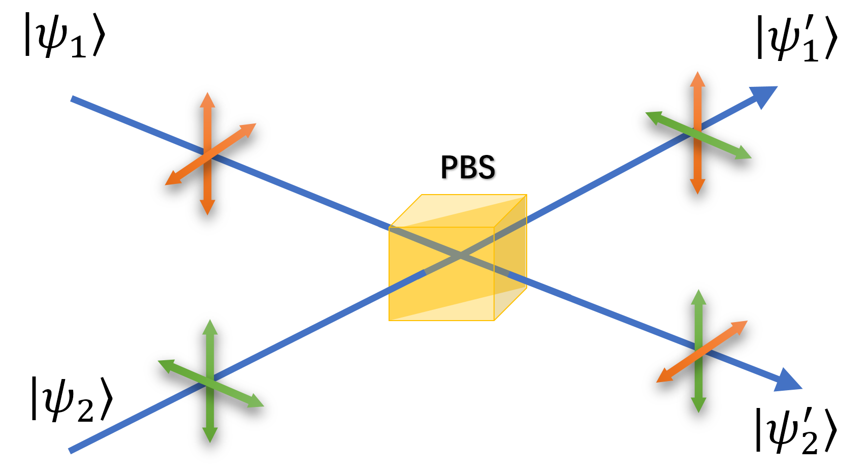
Figure 5: The scheme to exchange modes of two optical fields of Eq. (63) to imitate one of Bell states is shown, where PBS is  polarization beam splitter.

Then we obtain the results $\bar{P}(\theta_{a},k)=\cos(\theta_{a}+\gamma_{k}^{(a)})$ and $\bar{P}(\theta_{b},k)=\cos(\theta_{b}+\gamma_{k}^{(b)})$ for the measurement operators $\hat{P}\left(\theta_{a}\right)$ and $\hat{P}\left(\theta_{b}\right)$ locally performed on the fields $\left|\psi_{a}^{\prime}\right\rangle$ and$\ \left|\psi_{b}^{\prime}\right\rangle$, where $\gamma_{k}^{(a)},\gamma_{k}^{(b)}$ are the $k$-th units of the RPSs $\gamma^{(a)}$ and $\gamma^{(b)}$, respectively. Then the correlation function is

$$E(\theta_{a},\theta_{b})=\frac{1}{NC}\sum_{k=1}^{N}\bar{P}(\theta_{a},k)\bar{P}(\theta_{b},k)=\cos(\theta_{a}+\theta_{b}),$$ (68)

where $C=1/2$ is the normalization coefficient. The fields in Eq. (65) are considered to be the optical analogy to the Bell state $\left|\Psi^{+}\right\rangle$. By substituting the above correlation functions into Bell inequality (CHSH inequality) CHSH

$$\left|B\right|=\left|E(\theta_{a},\theta_{b})-E(\theta_{a},\theta_{b}^{\prime})+E(\theta_{a}^{\prime},\theta_{b}^{\prime})+E(\theta_{a}^{\prime},\theta_{b})\right|=2\sqrt{2}>2,$$ (69)

where $\theta_{a},\theta_{a}^{\prime},\theta_{b}$ and $\theta_{b}^{\prime}$ are $\pi/4,-\pi/4,0$ and $\pi/2$, respectively, Bell’s inequality is maximally violated.

Bell state $\left|\Psi^{+}\right\rangle$ differs from $\left|\Psi^{-}\right\rangle$ by $\pi$ phase. Similarly, the optical analogy to the Bell state $\left|\Psi^{-}\right\rangle$ is expressed as

$$\left|\psi_{a}^{\prime}\right\rangle = \frac{e^{i\lambda^{(a)}}}{\sqrt{2}}\left(\left|0\right\rangle+e^{i\gamma^{(a)}}\left|1\right\rangle\right),$$ (70)

$$\left|\psi_{b}^{\prime}\right\rangle = \frac{e^{i\lambda^{(b)}}}{\sqrt{2}}\left(\left|0\right\rangle+e^{i\left(\gamma^{(b)}+\pi\right)}\left|1\right\rangle\right).$$

By performing the transformation $\hat{\sigma}_{x}:\left|0\right\rangle\leftrightarrow\left|1\right\rangle$ on $\left|\psi_{b}^{\prime}\right\rangle$ of the state $\left|\Psi^{\pm}\right\rangle$, we obtain the optical analogy to the Bell state $\left|\Phi^{+}\right\rangle$ expressed as

$$\left|\psi_{a}^{\prime}\right\rangle = \frac{e^{i\lambda^{(a)}}}{\sqrt{2}}\left(\left|0\right\rangle+e^{i\gamma^{(a)}}\left|1\right\rangle\right),$$ (71)

$$\left|\psi_{b}^{\prime}\right\rangle = \frac{e^{i\lambda^{(b)}}}{\sqrt{2}}\left(\left|1\right\rangle+e^{i\gamma^{(b)}}\left|0\right\rangle\right),$$

and of $\left|\Phi^{-}\right\rangle$ expressed as

$$\left|\psi_{a}^{\prime}\right\rangle = \frac{e^{i\lambda^{(a)}}}{\sqrt{2}}\left(\left|0\right\rangle+e^{i\gamma^{(a)}}\left|1\right\rangle\right),$$ (72)

$$\left|\psi_{b}^{\prime}\right\rangle = \frac{e^{i\lambda^{(b)}}}{\sqrt{2}}\left(\left|1\right\rangle+e^{i\left(\gamma^{(b)}+\pi\right)}\left|0\right\rangle\right).$$

Then their correlation functions $E_{\Psi^{-}}\left(\theta_{a},\theta_{b}\right)=-\cos\left(\theta_{a}+\theta_{b}\right),E_{\Phi^{\pm}}\left(\theta_{a},\theta_{b}\right)=\pm\cos\left(\theta_{a}-\theta_{b}\right)$ are obtained. To substitute the correlation functions into Eq. (69), we also obtain the maximal violation of Bell’s inequality. The violation of Bell’s criterion demonstrates the nonlocal correlation of the two optical fields in our scheme, which results from shared randomness of the PPSs.

II.2.3 GHZ states: GHZ equality criterion

The nonlocality of the multipartite entangled GHZ states can in principle be manifest in a new criterion and need not be statistical as the violation of Bell inequality GHZ . Preparing three fields $\left|\psi_{a}\right\rangle,\left|\psi_{b}\right\rangle$ and $\left|\psi_{c}\right\rangle$ similar to Eq. (63), and cyclically exchanging the modes $\left|1\right\rangle$ of the fields, we obtain as follows

$$\left|\psi_{a}^{\prime}\right\rangle = \frac{1}{\sqrt{2}}\left(e^{i\lambda^{(a)}}\left|0\right\rangle+e^{i\lambda^{(b)}}\left|1\right\rangle\right)=\frac{e^{i\lambda^{(a)}}}{\sqrt{2}}\left(\left|0\right\rangle+e^{i\gamma^{(a)}}\left|1\right\rangle\right),$$ (73)

$$\left|\psi_{b}^{\prime}\right\rangle = \frac{1}{\sqrt{2}}\left(e^{i\lambda^{(b)}}\left|0\right\rangle+e^{i\lambda^{(c)}}\left|1\right\rangle\right)=\frac{e^{i\lambda^{(b)}}}{\sqrt{2}}\left(\left|0\right\rangle+e^{i\gamma^{(b)}}\left|1\right\rangle\right),$$

$$\left|\psi_{c}^{\prime}\right\rangle = \frac{1}{\sqrt{2}}\left(e^{i\lambda^{(c)}}\left|0\right\rangle+e^{i\lambda^{(a)}}\left|1\right\rangle\right)=\frac{e^{i\lambda^{(c)}}}{\sqrt{2}}\left(\left|0\right\rangle+e^{i\gamma^{(c)}}\left|1\right\rangle\right),$$

where the RPSs $\gamma^{(a)}=\lambda^{(b)}-\lambda^{(a)},\gamma^{(b)}=\lambda^{(c)}-\lambda^{(b)},\gamma^{(c)}=\lambda^{(a)}-\lambda^{(c)}$ and $\gamma^{(a)}+\gamma^{(b)}+\gamma^{(c)}=0$. The fields are considered to be the optical analogy to GHZ state $\left|\Psi\right\rangle=\frac{1}{\sqrt{2}}\left(\left|000\right\rangle+\left|111\right\rangle\right)$. We obtain the local measurement results $\bar{P}(\theta_{a},k)=\cos(\theta_{a}+\gamma_{k}^{(a)}),\bar{P}(\theta_{b},k)=\cos(\theta_{b}+\gamma_{k}^{(b)}),\bar{P}(\theta_{c},k)=\cos(\theta_{c}+\gamma_{k}^{(c)})$ for the fields $\left|\psi_{a}^{\prime}\right\rangle,\left|\psi_{b}^{\prime}\right\rangle$ and $\left|\psi_{c}^{\prime}\right\rangle$, respectively, and the correlation function can be obtained

$$E(\theta_{a},\theta_{b},\theta_{c})=\frac{1}{NC}\sum\limits_{k=1}^{N}\bar{P}(\theta_{a},k)\bar{P}(\theta_{b},k)\bar{P}(\theta_{c},k)=\cos(\theta_{a}+\theta_{b}+\theta_{c}),$$ (74)

where $C=1/4$ is the normalized coefficient. If $\theta_{a}+\theta_{b}+\theta_{c}=0,E(\theta_{a},\theta_{b},\theta_{c})=1$. If $\theta_{a}+\theta_{b}+\theta_{c}=\pi,E(\theta_{a},\theta_{b},\theta_{c})=-1$. By using GHZ State, the family of simple proofs of Bell’s theorem without inequalities can be obtained GHZ , which is different from the criterion of CHSH inequality CHSH . The sign of the correlation function can be also treated as the criterion, such as the negative correlation for nonlocal and the positive correlation for local when $\theta_{a}=\pi/3,\theta_{b}=\pi/3,\theta_{c}=\pi/3$. We also obtain the negative correlation using Eq. (74). The results are similar to the quantum case of GHZ states.

Further, the optical analogy to GHZ state could be generalized to the case of $N$ particles. By preparing $N$ optical fields similar to Eq. (63) and cyclically exchanging the modes $\left|1\right\rangle$, the fields can be obtained as follows

$$\left|\psi_{1}\right\rangle = e^{i\lambda^{\left(1\right)}}\left|0\right\rangle+e^{i\lambda^{\left(2\right)}}\left|1\right\rangle=e^{i\lambda^{\left(1\right)}}\left(\left|0\right\rangle+e^{i\gamma^{\left(1\right)}}\left|1\right\rangle\right),$$ (75)

$$\left|\psi_{2}\right\rangle = e^{i\lambda^{\left(2\right)}}\left|0\right\rangle+e^{i\lambda^{\left(3\right)}}\left|1\right\rangle=e^{i\lambda^{\left(2\right)}}\left(\left|0\right\rangle+e^{i\gamma^{\left(2\right)}}\left|1\right\rangle\right),$$

$$\vdots$$

$$\left|\psi_{N}\right\rangle = e^{i\lambda^{\left(N\right)}}\left|0\right\rangle+e^{i\lambda^{\left(1\right)}}\left|1\right\rangle=e^{i\lambda^{\left(N\right)}}\left(\left|0\right\rangle+e^{i\gamma^{\left(N\right)}}\left|1\right\rangle\right).$$

where the RPSs satisfy $\gamma^{(1)}+\cdots+\gamma^{(N)}=0$. We can obtain the correlation function

$$E(\theta_{1},\ldots,\theta_{N})=\frac{1}{NC}\sum\limits_{k=1}^{N}\bar{P}(\theta_{1},k)\ldots\bar{P}(\theta_{N},k)=\cos\left(\theta_{1}+\cdots+\theta_{N}\right),$$ (76)

where $\bar{P}(\theta_{i},k)=\cos(\theta_{i}+\gamma_{k}^{(i)})$ are the local measurement results of the optical fields $\left|\psi_{i}\right\rangle$, and $C=1/2^{N-1}$ is the normalized coefficient.

Using the same notion, we can obtain optical analogy results of other quantum entanglement states. It should be pointed out that the phase randomness provided by PPSs is different from the case of quantum mixed states. Quantum mixed states result from decoherence and all coherent superposition items (non-diagonal terms) disappear. In contract to the decoherence, some coherent superposition items remain in the optical analogy state due to the constraints of the RPSs, such as $\gamma^{(a)}+\gamma^{(b)}=0,\gamma^{(a)}+\gamma^{(b)}+\gamma^{(c)}=0$ for the analogies to Bell states and GHZ state, respectively. These remaining items make it possible to imitate quantum entangled pure states.

II.2.4 Numerical simulation for the optical analogy to quantum entanglement

Here we numerically simulate the optical analogy to quantum entanglement by using the software OPTISYSTEM. First we propose the scheme to produce the product state of Eq. (63) shown in Fig. 6. In the scheme, we choose two sequences $\lambda_{k}^{\left(1\right)}$ and $\lambda_{k}^{\left(2\right)}$ from the set $\Xi$ to modulate the optical fields, and obtain

$$E_{1}\left(t\right) = \left(A_{\uparrow}+A_{\rightarrow}\right)e^{-i\left(\omega t+\lambda_{k}^{\left(1\right)}\right)},$$ (77)

$$E_{2}\left(t\right) = \left(A_{\uparrow}+A_{\rightarrow}\right)e^{-i\left(\omega t+\lambda_{k}^{\left(2\right)}\right)},$$

where $A_{\uparrow}$ and $A_{\rightarrow}$ denote the amplitudes of two orthogonal polarization modes $\left|0\right\rangle$ and $\left|1\right\rangle$, respectively.

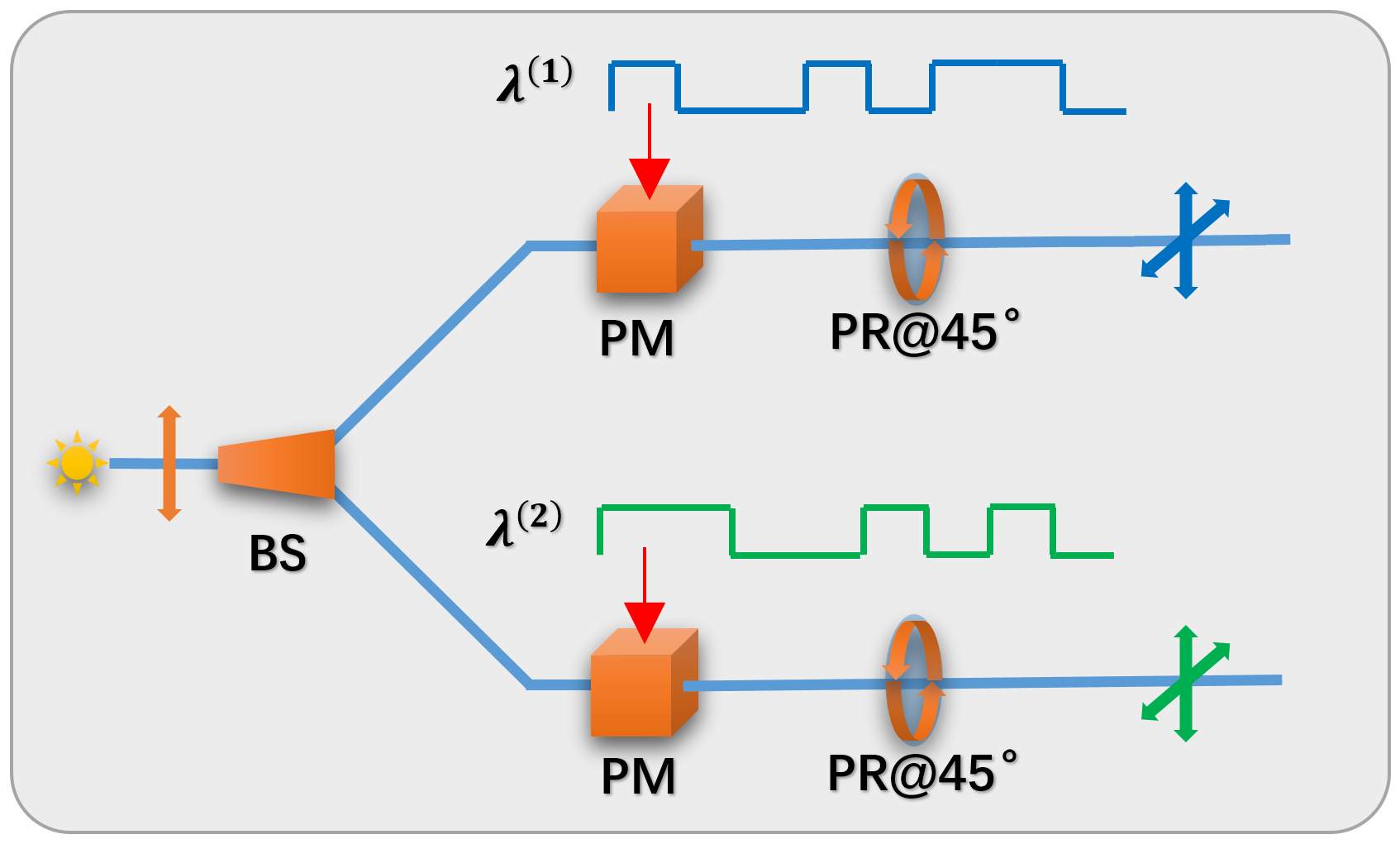
Figure 6: The sheme to realize the simulation of quantum product state is shown, where PR@$45^{\circ}$: $45^{\circ}$ polarization rotators.

After mode exchanged as shown in Fig. 5, the optical fields can be written as follows

$$E_{1}\left(t\right) = A_{\uparrow}e^{-i\left(\omega t+\lambda_{k}^{\left(1\right)}\right)}+A_{\rightarrow}e^{-i\left(\omega t+\lambda_{k}^{\left(2\right)}\right)},$$ (78)

$$E_{2}\left(t\right) = A_{\uparrow}e^{-i\left(\omega t+\lambda_{k}^{\left(2\right)}\right)}+A_{\rightarrow}e^{-i\left(\omega t+\lambda_{k}^{\left(1\right)}\right)}.$$

The numerical simulation scheme of the correlation measurement is shown in Fig. 7. First, two modes of $E_{1}\left(t\right)$ and $E_{2}\left(t\right)$ are modulated with phase differences $\theta_{1}$ and $\theta_{2}$, respectively. The fields can be written as follows

$$E_{1}\left(t\right) = A_{\uparrow}e^{-i\left(\omega t+\lambda_{k}^{\left(1\right)}+\theta_{1}/2\right)}+A_{\rightarrow}e^{-i\left(\omega t+\lambda_{k}^{\left(2\right)}-\theta_{1}/2\right)},$$ (79)

$$E_{2}\left(t\right) = A_{\uparrow}e^{-i\left(\omega t+\lambda_{k}^{\left(2\right)}+\theta_{2}/2\right)}+A_{\rightarrow}e^{-i\left(\omega t+\lambda_{k}^{\left(1\right)}-\theta_{2}/2\right)}.$$

Then the fields $E_{1}\left(t\right)$ and $E_{2}\left(t\right)$ are split two beams by the polarization beamsplitters at angles $45^{\circ}$ and input the photodetectors $\left(D_{1},D_{2}\right)$ and $\left(D_{3},D_{4}\right)$, respectively. The differential signals of photodetectors are proportional to

$$I_{1} = \left|D_{1}\right|^{2}-\left|D_{2}\right|^{2}=\mu\left|A_{s}\right|^{2}\cos\left(\lambda_{k}^{\left(1\right)}-\lambda_{k}^{\left(2\right)}+\theta_{1}\right),$$ (80)

$$I_{2} = \left|D_{3}\right|^{2}-\left|D_{4}\right|^{2}=\mu\left|A_{s}\right|^{2}\cos\left(\lambda_{k}^{\left(2\right)}-\lambda_{k}^{\left(1\right)}+\theta_{2}\right),$$

where $\left|D_{i}\right|^{2}$ are the output electric signals of the photodetectors, $A_{s}=A_{\uparrow}=A_{\rightarrow}$ assumed. Then we calculate the correlation function $E(\theta_{1},\theta_{2})=\left\langle I_{1}I_{2}\right\rangle/C=\cos\left(\theta_{1}+\theta_{2}\right)$, where $C=4\mu^{2}\left|A_{s}\right|^{4}\Delta T$ is the normalization coefficient. Finally, using the software OPTISYSTEM, we obtain the numerical results of the normalized correlation function as shown in Fig. 8 (Detailed simulation data and OPTISYSTEM models will be provided in the supplementary material). By substituting the above correlation results into Bell inequality (CHSH inequality) CHSH : $\left|B\right|=2.825\pm 0.001>2$ where $\theta_{1},\theta_{1}^{\prime},\theta_{2}$ and $\theta_{2}^{\prime}$ are $\pi/4,-\pi/4,0$ and $\pi/2$, respectively.

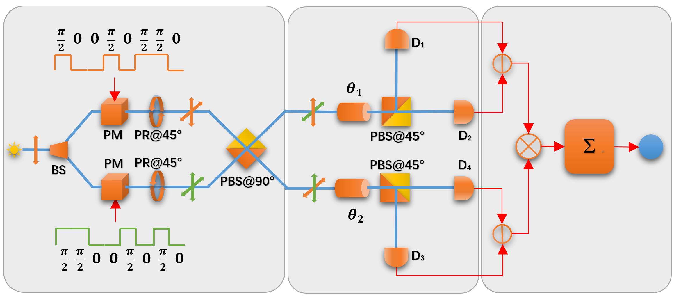
Figure 7: The scheme to realize the correlation measurement of quantum entanglement state is shown, where $\theta_{1}$ and $\theta_{2}$ are the modulators to produce phase differences between two polarization modes; PBS$@45^{\circ}$ and PBS$@90^{\circ}$ polarization beam splitters at $45^{\circ}$ and $90^{\circ}$ respectively; PR@$45^{\circ}$: $45^{\circ}$ polarization rotators.

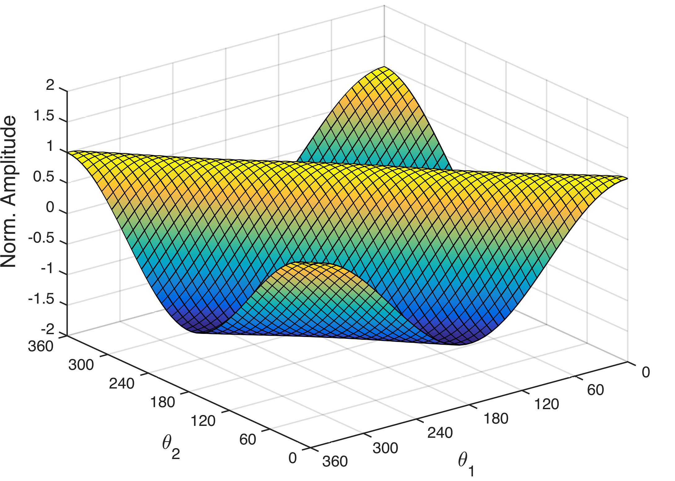
Figure 8: The result of the correlation function for the analogy to one of Bell states is shown.

II.3 Optical analogies to quantum states of multiple particles

We have discussed the coherent demodulation process in Sec. I.2. Here we discuss how to imitate quantum states with the help of the coherent demodulation.

First, we consider the general form of $N$ optical fields modulated with PPSs $\left\{\lambda^{\left(1\right)},\ldots,\lambda^{\left(N\right)}\right\}$ chosen from the set $\Xi$, and the states can be expressed as Eq. (45). It is noteworthy that although multiple PPSs are superimposed on two orthogonal modes of the fields, all of the PPSs can be demodulated and discriminated by respectively performing the coherent demodulations on the two orthogonal modes, which has already been verified by many actual communication systems Viterbi ; Peterson ; PSK .

Now we propose a scheme, as shown in Fig. 9, to perform the coherent demodulation introduced in Sec. I.2. In the scheme, the coherent demodulations are performed on each SO field and LO field modulated with reference PPSs $\left\{\lambda^{\left(1\right)},\ldots,\lambda^{\left(N\right)}\right\}$. Thus a mode status matrix $M\left(\tilde{\alpha}_{i}^{j},\tilde{\beta}_{i}^{j}\right)$, as shown in Fig. 10, can be obtained by performing $N$ coherent demodulations on each SO field, where $\tilde{\alpha}_{i}^{j},\tilde{\beta}_{i}^{j}$ are the mode status of the orthogonal polarization modes $\left|0\right\rangle$ and $\left|1\right\rangle$, respectively. For better fault tolerance, the mode status output discrete values through the threshold discrimination and binarization of the measurement results. Of the matrix $M\left(\tilde{\alpha}_{i}^{j},\tilde{\beta}_{i}^{j}\right)$, each element represents the mode status of the $i$th optical field when the reference PPS is $\lambda^{\left(j\right)}$, and takes one of four possible discrete values: $\left(1,0\right),\left(0,1\right),\left(1,1\right)$ or $0$, denoting that exists only mode $\left|0\right\rangle$, only mode $\left|1\right\rangle$, both $\left|0\right\rangle$ and $\left|1\right\rangle$, neither $\left|0\right\rangle$ nor $\left|1\right\rangle$, respectively. Thus we obtain a one-to-one correspondence relationship between the $N$ optical fields and the matrix $M$. Thus we consider the matrix $M$ as a bridge to connect the optical fields and the quantum states.

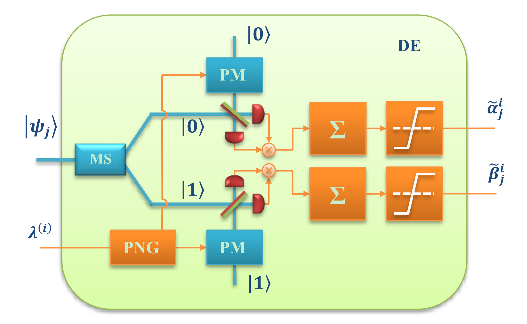
Figure 9: The coherent demodulation scheme of pseudorandom phase sequence is shown, where SO: signal optical fields, LO: local optical fields, MS: mode splitters, PM: phase modulators, PNG: pseudorandom number generators, $\otimes$: multipliers and $\Sigma$: integrators (integrate over entire sequence period).

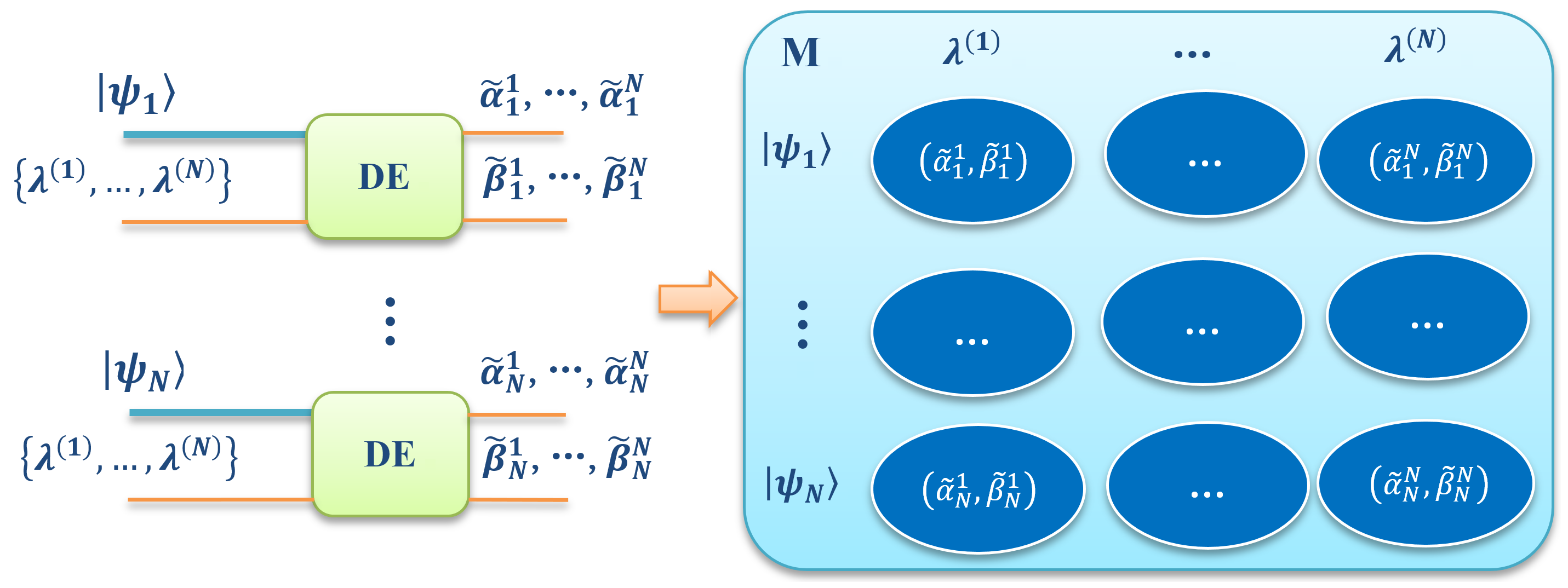
Figure 10: The PPS coherent demodulation scheme for multiple input fields is shown, where the DE block is shown in Fig. 9.

Now we discuss how to construct the imitation states based on the matrix $M$. In the subsection II.1.3, we propose the SCPM to reduce the redundancy of sequential permutation. Here we apply the SCPM to imitate quantum states based on the $M$ matrix. In order to clearly present the SCPM in the $M$ matrix, as shown in Fig. 11, the matrix elements belonging to the same permutation $R_{r}$ are labeled with the same color, such as the red color corresponding to $R_{1}$, the blue color corresponding to $R_{2}$, etc. Considering each permutation $R_{r}$ corresponding to equivalent direct product decompositions, thus the imitated quantum state must be a direct product of the elements belonging to the same $R_{r}$ and then superposition of equivalent direct products corresponding to all permutations. Therefore we obtain

$$\left|\Psi\right\rangle = \left(\tilde{\alpha}_{1}^{1}\left|0\right\rangle+\tilde{\beta}_{1}^{1}\left|1\right\rangle\right)\otimes\ldots\otimes\left(\tilde{\alpha}_{N}^{N}\left|0\right\rangle+\tilde{\beta}_{N}^{N}\left|1\right\rangle\right)+\left(\tilde{\alpha}_{1}^{2}\left|0\right\rangle+\tilde{\beta}_{1}^{2}\left|1\right\rangle\right)\otimes\ldots\otimes\left(\tilde{\alpha}_{N}^{1}\left|0\right\rangle+\tilde{\beta}_{N}^{1}\left|1\right\rangle\right)$$

$$+\ldots+\left(\tilde{\alpha}_{1}^{N}\left|0\right\rangle+\tilde{\beta}_{1}^{N}\left|1\right\rangle\right)\otimes\ldots\otimes\left(\tilde{\alpha}_{N}^{N-1}\left|0\right\rangle+\tilde{\beta}_{N}^{N-1}\left|1\right\rangle\right),$$

where $\tilde{\alpha}_{i}^{j},\tilde{\beta}_{i}^{j}$ is the mode discrete status obtained from the matrix $M\left(\tilde{\alpha}_{i}^{j},\tilde{\beta}_{i}^{j}\right)$.

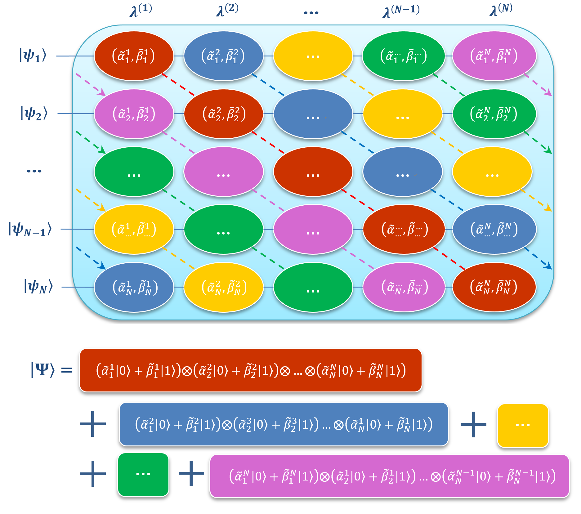
Figure 11: The scheme to imitate quantum state is shown, the mode status matrix $M\left(\tilde{\alpha}_{i}^{j},\tilde{\beta}_{i}^{j}\right)$ related to the $i$th optical field and the reference PPS $\lambda^{\left(j\right)}$, in which the mode status with the same color for the same sequence permutation.

It is noteworthy that the SCPM to reduce the redundancy is one of the feasible ways to imitate quantum states based on the matrix $M$. Other mechanisms might also work, as long as a sequential ergodic ensemble can be obtained. In order to prove the feasibility of the scheme, in the next subsection, we will discuss the imitations of several typical quantum states, including the product states, Bell states, GHZ states and W states.

II.3.1 The imitation states of several typical quantum states

In this subsection, we discuss optical analogies to several typical quantum states and construct their imitation states applying the scheme proposed in the last subsection, including the product state, Bell states, GHZ state and W state.

The product state

First, we discuss the optical analogy to the product state of $N$ qubit. The optical fields are shown as follows

$$\left|\psi_{1}\right\rangle = e^{i\lambda^{\left(1\right)}}\left(\left|0\right\rangle+\left|1\right\rangle\right),$$

$$\vdots$$

$$\left|\psi_{N}\right\rangle = e^{i\lambda^{\left(N\right)}}\left(\left|0\right\rangle+\left|1\right\rangle\right).$$

By employing the scheme as shown in Fig. 11, we obtain the matrix

$$M\left(\tilde{\alpha}_{i}^{j},\tilde{\beta}_{i}^{j}\right)=\left(\begin{array}[]{ccc}\left(1,1\right)&&\\ &\ddots&\\ &&\left(1,1\right)\end{array}\right),$$ (83)

which demonstrates that each optical field is the superposition of two orthogonal modes and no entanglement is involved. According to Eq. (II.3), we obtain the imitation state as follow

$$\left|\Psi\right\rangle = \left(\left|0\right\rangle+\left|1\right\rangle\right)\otimes\ldots\otimes\left(\left|0\right\rangle+\left|1\right\rangle\right)$$

$$= \left|0\ldots 0\right\rangle+\left|0\ldots 1\right\rangle+\ldots+\left|1\ldots 1\right\rangle,$$

which is same as the quantum product state expect a normalization factor.

Bell states

Now we discuss the optical analogy to one of the four Bell states $\left|\Psi^{+}\right\rangle=\frac{1}{\sqrt{2}}\left(\left|00\right\rangle+\left|11\right\rangle\right)$, which contains two optical fields as Eq. (65). By employing the scheme as shown in Fig. 11, we obtain the matrix

$$M\left(\tilde{\alpha}_{i}^{j},\tilde{\beta}_{i}^{j}\right)=\left(\begin{array}[]{cc}\left(1,0\right)&\left(0,1\right)\\ \left(0,1\right)&\left(1,0\right)\end{array}\right).$$ (85)

According to the SCPM, we obtain that $R_{1}=\{\lambda^{\left(1\right)},\lambda^{\left(2\right)}\}$ and $R_{2}=\{\lambda^{\left(2\right)},\lambda^{\left(1\right)}\}$. Based on the matrix $M$, for the selection of $R_{1}$, we obtain the modes of the fields are $\left|0\right\rangle$ and $\left|0\right\rangle$; for the selection of $R_{2}$, we obtain the modes are $\left|1\right\rangle$ and $\left|1\right\rangle$. If we randomly choose $R_{1}$ or $R_{2}$, we can randomly obtain the mode status of $\left|0\right\rangle\left|0\right\rangle$ or $\left|1\right\rangle\left|1\right\rangle$, which is similar to quantum measurements for the Bell state $\left|\Psi^{+}\right\rangle$. According to Eq. (II.3), we obtain the imitation state as follow

$$\left|\Psi\right\rangle = \left(\tilde{\alpha}_{1}^{1}\left|0\right\rangle+\tilde{\beta}_{1}^{1}\left|1\right\rangle\right)\otimes\left(\tilde{\alpha}_{2}^{2}\left|0\right\rangle+\tilde{\beta}_{2}^{2}\left|1\right\rangle\right)+\left(\tilde{\alpha}_{1}^{2}\left|0\right\rangle+\tilde{\beta}_{1}^{2}\left|1\right\rangle\right)\otimes\left(\tilde{\alpha}_{2}^{1}\left|0\right\rangle+\tilde{\beta}_{2}^{1}\left|1\right\rangle\right)$$

$$= \left|00\right\rangle+\left|11\right\rangle,$$

which is same as the Bell state $\left|\Psi^{+}\right\rangle$ expect a normalization factor.

We discuss the optical analogy to another Bell state $\left|\Phi^{+}\right\rangle$, which contains two optical fields as Eq. (71). We then obtain the matrix

$$M\left(\tilde{\alpha}_{i}^{j},\tilde{\beta}_{i}^{j}\right)=\left(\begin{array}[]{cc}\left(1,0\right)&\left(0,1\right)\\ \left(1,0\right)&\left(0,1\right)\end{array}\right).$$ (87)

If we randomly choose $R_{1}$ or $R_{2}$, we can also randomly obtain the mode results $\left|0\right\rangle\left|1\right\rangle$ or $\left|0\right\rangle\left|1\right\rangle$, which is similar to quantum measurement for the Bell state $\left|\Phi^{+}\right\rangle$. We can obtain the imitation state

$$\left|\Psi\right\rangle = \left(\tilde{\alpha}_{1}^{1}\left|0\right\rangle+\tilde{\beta}_{1}^{1}\left|1\right\rangle\right)\otimes\left(\tilde{\alpha}_{2}^{2}\left|0\right\rangle+\tilde{\beta}_{2}^{2}\left|1\right\rangle\right)+\left(\tilde{\alpha}_{1}^{2}\left|0\right\rangle+\tilde{\beta}_{1}^{2}\left|1\right\rangle\right)\otimes\left(\tilde{\alpha}_{2}^{1}\left|0\right\rangle+\tilde{\beta}_{2}^{1}\left|1\right\rangle\right)$$

$$= \left|10\right\rangle+\left|01\right\rangle,$$

which is same as the Bell state $\left|\Phi^{+}\right\rangle$ expect a normalization factor.

GHZ state

For tripartite systems there are only two different classes of genuine tripartite entanglement, the GHZ class and the W class GHZ ; Nielsen . First we discuss the optical analogy to GHZ state $\left|\Psi_{GHZ}\right\rangle=\frac{1}{\sqrt{2}}\left(\left|000\right\rangle+\left|111\right\rangle\right)$, which contains three optical fields as Eq. (73), where the superscripts of the PPSs become $1,2,3$. We obtain the matrix

$$M\left(\tilde{\alpha}_{i}^{j},\tilde{\beta}_{i}^{j}\right)=\left(\begin{array}[]{ccc}\left(1,0\right)&\left(0,1\right)&0\\ 0&\left(1,0\right)&\left(0,1\right)\\ \left(0,1\right)&0&\left(1,0\right)\end{array}\right).$$ (89)

According to the SCPM, we obtain that $R_{1}=\{\lambda^{\left(1\right)},\lambda^{\left(2\right)},\lambda^{\left(3\right)}\}$, $R_{2}=\{\lambda^{\left(2\right)},\lambda^{\left(3\right)},\lambda^{\left(1\right)}\}$ and $R_{3}=\{\lambda^{\left(3\right)},\lambda^{\left(1\right)},\lambda^{\left(2\right)}\}$. Based on the matrix $M$, for the selection of $R_{1}$, we obtain the mode status are $\left|0\right\rangle\left|0\right\rangle\left|0\right\rangle$; for the selection of $R_{2}$, we obtain the mode status are $\left|1\right\rangle\left|1\right\rangle\left|1\right\rangle$; for the selection of $R_{3}$, we obtain nothing. Thus we can obtain the imitation state

$$\left|\Psi\right\rangle = \left(\tilde{\alpha}_{1}^{1}\left|0\right\rangle+\tilde{\beta}_{1}^{1}\left|1\right\rangle\right)\otimes\left(\tilde{\alpha}_{2}^{2}\left|0\right\rangle+\tilde{\beta}_{2}^{2}\left|1\right\rangle\right)\otimes\left(\tilde{\alpha}_{3}^{3}\left|0\right\rangle+\tilde{\beta}_{3}^{3}\left|1\right\rangle\right)$$

$$+\left(\tilde{\alpha}_{1}^{2}\left|0\right\rangle+\tilde{\beta}_{1}^{2}\left|1\right\rangle\right)\otimes\left(\tilde{\alpha}_{2}^{3}\left|0\right\rangle+\tilde{\beta}_{2}^{3}\left|1\right\rangle\right)\otimes\left(\tilde{\alpha}_{3}^{1}\left|0\right\rangle+\tilde{\beta}_{3}^{1}\left|1\right\rangle\right)$$

$$= \left|000\right\rangle+\left|111\right\rangle.$$

For $N$ quantum particles, we can obtain the analogy to GHZ state $\left|\Psi_{GHZ}\right\rangle=\frac{1}{\sqrt{2}}\left(\left|0...0\right\rangle+\left|1...1\right\rangle\right)$, which contains $N$ optical fields as Eq. (75). Performing the scheme as shown in Fig. 11, we obtain the matrix

$$M\left(\tilde{\alpha}_{i}^{j},\tilde{\beta}_{i}^{j}\right)=\left(\begin{array}[]{ccccc}\left(1,0\right)&\left(0,1\right)&&&\\ &\left(1,0\right)&\left(0,1\right)&&\\ &&\ddots&\ddots&\\ &&&\left(1,0\right)&\left(0,1\right)\\ \left(0,1\right)&&&&\left(1,0\right)\end{array}\right).$$ (91)

Thus we can easily obtain the imitation state same as GHZ state $\left|\Psi_{GHZ}\right\rangle$ expect a normalization factor.

In the following, we discuss any unitary transformation states of GHZ state. Assuming the unitary transformation simplified from Eq. (38),

$$\hat{U}\left|\psi\right\rangle = \hat{U}\left(\alpha\left|0\right\rangle+\beta\left|1\right\rangle\right)$$

$$= \alpha\left(C_{0}\left|0\right\rangle+C_{1}\left|1\right\rangle\right)+\beta\left(C_{0}^{\ast}\left|1\right\rangle-C_{1}^{\ast}\left|0\right\rangle\right),$$

we employ it on GHZ state of $N$ quantum particles and obtain as follow

$$\hat{U}_{n}\left|\Psi_{GHZ}\right\rangle=\frac{1}{\sqrt{2}}\left[C_{0}\left|0...0_{n}...0\right\rangle+C_{1}\left|0...1_{n}...0\right\rangle+C_{0}^{\ast}\left|1...1_{n}...1\right\rangle-C_{1}^{\ast}\left|1...0_{n}...1\right\rangle\right].$$ (93)

Similarly, we employ the transformation on the optical analogy fields as follows

$$\left|\psi_{1}\right\rangle = e^{i\lambda^{\left(1\right)}}\left|0\right\rangle+e^{i\lambda^{\left(2\right)}}\left|1\right\rangle,$$

$$\vdots$$

$$\hat{U}_{n}\left|\psi_{n}\right\rangle = e^{i\lambda^{\left(n\right)}}\left(C_{0}\left|0\right\rangle+C_{1}\left|1\right\rangle\right)+e^{i\lambda^{\left(n+1\right)}}\left(C_{0}^{\ast}\left|1\right\rangle-C_{1}^{\ast}\left|0\right\rangle\right),$$

$$\vdots$$

$$\left|\psi_{N}\right\rangle = e^{i\lambda^{\left(N\right)}}\left|0\right\rangle+e^{i\lambda^{\left(1\right)}}\left|1\right\rangle.$$

We obtain the matrix

$$M\left(\tilde{\alpha}_{i}^{j},\tilde{\beta}_{i}^{j}\right)=\left(\begin{array}[]{ccccc}\left(1,0\right)&\left(0,1\right)&&&\\ &\ddots&\ddots&&\\ &&\left(C_{0},C_{1}\right)&\left(-C_{1}^{\ast},C_{0}^{\ast}\right)&\\ &&&\ddots&\ddots\\ \left(0,1\right)&&&&\left(1,0\right)\end{array}\right),$$ (95)

and the imitation state

$$\left|\Psi\right\rangle=C_{0}\left|0...0_{n}...0\right\rangle+C_{1}\left|0...1_{n}...0\right\rangle+C_{0}\left|1...1_{n}...1\right\rangle-C_{1}^{\ast}\left|1...0_{n}...1\right\rangle.$$ (96)

Obviously, we can obtain the result completely similar to quantum states. For a simple case, we discuss the NOT unitary transformation $\hat{U}_{NOT}\left|\psi_{n}\right\rangle\rightarrow\hat{U}_{NOT}\left(\alpha_{n}\left|0\right\rangle+\beta_{n}\left|1\right\rangle\right)=\alpha_{n}\left|1\right\rangle+\beta_{n}\left|0\right\rangle$ as follows

$$\left|\psi_{1}\right\rangle = e^{i\lambda^{\left(1\right)}}\left|0\right\rangle+e^{i\lambda^{\left(2\right)}}\left|1\right\rangle,$$

$$\left|\psi_{2}\right\rangle = e^{i\lambda^{\left(2\right)}}\left|0\right\rangle+e^{i\lambda^{\left(3\right)}}\left|1\right\rangle,$$

$$\vdots$$

$$\hat{U}_{NOT}\left|\psi_{n}\right\rangle = \hat{U}_{NOT}\left(e^{i\lambda^{\left(n\right)}}\left|0\right\rangle+e^{i\lambda^{\left(n+1\right)}}\left|1\right\rangle\right)=e^{i\lambda^{\left(n\right)}}\left|1\right\rangle+e^{i\lambda^{\left(n+1\right)}}\left|0\right\rangle,$$

$$\vdots$$

$$\left|\psi_{N}\right\rangle = e^{i\lambda^{\left(N\right)}}\left|0\right\rangle+e^{i\lambda^{\left(1\right)}}\left|1\right\rangle,$$

and the transformed imitation state can be expressed as follow

$$\left|\Psi\right\rangle=\left|00...1_{n}...0\right\rangle+\left|11...0_{n}...1\right\rangle.$$ (97)

Similar to quantum computation, we can obtain a new state by using only one step instead of $2$ steps as classical computation. This is a simple example to demonstrate parallel computing capability.

W state

Now we discuss the optical analogy to W state $\left|\Psi_{W}\right\rangle=\frac{1}{\sqrt{3}}\left(\left|100\right\rangle+\left|010\right\rangle+\left|001\right\rangle\right)$, which contains three optical fields as follows

$$\left|\psi_{1}\right\rangle = e^{i\lambda^{\left(1\right)}}\left|1\right\rangle+e^{i\lambda^{\left(2\right)}}\left|0\right\rangle+e^{i\lambda^{\left(3\right)}}\left|0\right\rangle,$$ (98)

$$\left|\psi_{2}\right\rangle = e^{i\lambda^{\left(1\right)}}\left|1\right\rangle+e^{i\lambda^{\left(2\right)}}\left|0\right\rangle+e^{i\lambda^{\left(3\right)}}\left|0\right\rangle,$$

$$\left|\psi_{3}\right\rangle = e^{i\lambda^{\left(1\right)}}\left|1\right\rangle+e^{i\lambda^{\left(2\right)}}\left|0\right\rangle+e^{i\lambda^{\left(3\right)}}\left|0\right\rangle.$$

Performing the same scheme in Fig. 11, we obtain the matrix

$$M\left(\tilde{\alpha}_{i}^{j},\tilde{\beta}_{i}^{j}\right)=\left(\begin{array}[]{ccc}\left(0,1\right)&\left(1,0\right)&\left(1,0\right)\\ \left(0,1\right)&\left(1,0\right)&\left(1,0\right)\\ \left(0,1\right)&\left(1,0\right)&\left(1,0\right)\end{array}\right).$$ (99)

According to the SCPM, we use $R_{1}$, $R_{2}$ and $R_{3}$ again. Based on the matrix $M$, we obtain the mode status of $\left|1\right\rangle\left|0\right\rangle\left|0\right\rangle$, $\left|0\right\rangle\left|0\right\rangle\left|1\right\rangle$, $\left|0\right\rangle\left|1\right\rangle\left|0\right\rangle$ for the selection of $R_{1}$, $R_{2}$, $R_{3}$, respectively. We find an interesting fact that if we need to lock the mode status $\left|1\right\rangle$ for the first field, $R_{1}$ must be selected. This will lead to the mode status $\left|0\right\rangle\left|0\right\rangle$ must be obtained from the other two fields. Otherwise if the state status $\left|0\right\rangle$ of the first field is obtain, $R_{2}$ or $R_{3}$ can be selected. This will lead to the other two fields are still in the state $\left|0\right\rangle\left|1\right\rangle+\left|1\right\rangle\left|0\right\rangle$ similar to Bell state $\left|\Phi^{+}\right\rangle$. This fact is quite similar to the case of quantum measurement and the collapse phenomenon for W state in quantum mechanics. We obtain the imitation state as follow

$$\left|\Psi\right\rangle = \left(\tilde{\alpha}_{1}^{1}\left|0\right\rangle+\tilde{\beta}_{1}^{1}\left|1\right\rangle\right)\otimes\left(\tilde{\alpha}_{2}^{2}\left|0\right\rangle+\tilde{\beta}_{2}^{2}\left|1\right\rangle\right)\otimes\left(\tilde{\alpha}_{3}^{3}\left|0\right\rangle+\tilde{\beta}_{3}^{3}\left|1\right\rangle\right)$$

$$+\left(\tilde{\alpha}_{1}^{2}\left|0\right\rangle+\tilde{\beta}_{1}^{2}\left|1\right\rangle\right)\otimes\left(\tilde{\alpha}_{2}^{3}\left|0\right\rangle+\tilde{\beta}_{2}^{3}\left|1\right\rangle\right)\otimes\left(\tilde{\alpha}_{3}^{1}\left|0\right\rangle+\tilde{\beta}_{3}^{1}\left|1\right\rangle\right)$$

$$+\left(\tilde{\alpha}_{1}^{3}\left|0\right\rangle+\tilde{\beta}_{1}^{3}\left|1\right\rangle\right)\otimes\left(\tilde{\alpha}_{2}^{1}\left|0\right\rangle+\tilde{\beta}_{2}^{1}\left|1\right\rangle\right)\otimes\left(\tilde{\alpha}_{3}^{2}\left|0\right\rangle+\tilde{\beta}_{3}^{2}\left|1\right\rangle\right)$$

$$= \left|100\right\rangle+\left|010\right\rangle+\left|001\right\rangle.$$

For $N$ quantum particles, we can obtain the analogy to W state $\left|\Psi_{W}\right\rangle=\frac{1}{\sqrt{N}}\left(\left|10...0\right\rangle+\left|01...0\right\rangle+...+\left|00...1\right\rangle\right)$, which contains $N$ optical fields as follows

$$\left|\psi_{1}\right\rangle = e^{i\lambda^{\left(1\right)}}\left|1\right\rangle+e^{i\lambda^{\left(2\right)}}\left|0\right\rangle+...+e^{i\lambda^{\left(N\right)}}\left|0\right\rangle,$$ (101)

$$\left|\psi_{2}\right\rangle = e^{i\lambda^{\left(1\right)}}\left|1\right\rangle+e^{i\lambda^{\left(2\right)}}\left|0\right\rangle+...+e^{i\lambda^{\left(N\right)}}\left|0\right\rangle,$$

$$\vdots$$

$$\left|\psi_{N}\right\rangle = e^{i\lambda^{\left(1\right)}}\left|1\right\rangle+e^{i\lambda^{\left(2\right)}}\left|0\right\rangle+...+e^{i\lambda^{\left(N\right)}}\left|0\right\rangle.$$

Now we discuss a transformed state of W state. Applying the NOT unitary transformation $\hat{U}_{NOT}:\left|0\right\rangle\leftrightarrow\left|1\right\rangle$ to $\left|\psi_{n}\right\rangle$, we can obtain the transformed optical fields as follows

$$\left|\psi_{1}\right\rangle = e^{i\lambda^{\left(1\right)}}\left|1\right\rangle+e^{i\lambda^{\left(2\right)}}\left|0\right\rangle+...+e^{i\lambda^{\left(N\right)}}\left|0\right\rangle,$$

$$\vdots$$

$$\hat{U}_{NOT}\left|\psi_{n}\right\rangle = \hat{U}_{NOT}\left(e^{i\lambda^{\left(1\right)}}\left|1\right\rangle+e^{i\lambda^{\left(2\right)}}\left|0\right\rangle+...+e^{i\lambda^{\left(N\right)}}\left|0\right\rangle\right)=e^{i\lambda^{\left(1\right)}}\left|0\right\rangle+e^{i\lambda^{\left(2\right)}}\left|1\right\rangle+...+e^{i\lambda^{\left(N\right)}}\left|1\right\rangle,$$

$$\vdots$$

$$\left|\psi_{N}\right\rangle = e^{i\lambda^{\left(1\right)}}\left|1\right\rangle+e^{i\lambda^{\left(2\right)}}\left|0\right\rangle+...+e^{i\lambda^{\left(N\right)}}\left|0\right\rangle.$$

and the transformed imitation state can be expressed as

$$\left|\Psi\right\rangle=\left|10...1_{n}...00\right\rangle+...+\left|00...0_{n}...00\right\rangle+...+\left|00...1_{n}...01\right\rangle.$$ (103)

Similar to quantum computation, we can obtain a new state by using only one step instead of $N$ steps as classical computation. This is another example to demonstrate parallel computing capability.

II.3.2 Numerical simulations of the optical analogies to the three-particle quantum states

In last subsection, we demonstrate the optical analogies of quantum states, which are the product state, Bell states, GHZ state and W state. In this subsection, we discuss numerical simulations of two optical analogies using the software OPTISYSTEM. To construct the product state, we first choose three PPSs $\lambda^{\left(1\right)},\lambda^{\left(2\right)}$ and $\lambda^{\left(3\right)}$ to modulate the optical fields, and obtain

$$E_{1}\left(t\right) = \left(A_{\uparrow}+A_{\rightarrow}\right)e^{-i\left(\omega t+\lambda_{k}^{\left(1\right)}\right)},$$ (104)

$$E_{2}\left(t\right) = \left(A_{\uparrow}+A_{\rightarrow}\right)e^{-i\left(\omega t+\lambda_{k}^{\left(2\right)}\right)},$$

$$E_{3}\left(t\right) = \left(A_{\uparrow}+A_{\rightarrow}\right)e^{-i\left(\omega t+\lambda_{k}^{\left(3\right)}\right)}.$$

According to Eq. (73), the optical analogies to GHZ state can be written as follows

$$E_{1}\left(t\right) = A_{\uparrow}e^{-i\left(\omega t+\lambda_{k}^{\left(1\right)}\right)}+A_{\rightarrow}e^{-i\left(\omega t+\lambda_{k}^{\left(2\right)}\right)},$$ (105)

$$E_{2}\left(t\right) = A_{\uparrow}e^{-i\left(\omega t+\lambda_{k}^{\left(2\right)}\right)}+A_{\rightarrow}e^{-i\left(\omega t+\lambda_{k}^{\left(3\right)}\right)},$$

$$E_{3}\left(t\right) = A_{\uparrow}e^{-i\left(\omega t+\lambda_{k}^{\left(3\right)}\right)}+A_{\rightarrow}e^{-i\left(\omega t+\lambda_{k}^{\left(1\right)}\right)},$$

which can be realized by mode exchange of the produce state by using polarization beam splitters, as shown in Fig. 12. Then we can express the optical analogies to W state as follows

$$E_{1}\left(t\right) = A_{\rightarrow}e^{-i\left(\omega t+\lambda_{k}^{\left(1\right)}\right)}+A_{\uparrow}e^{-i\left(\omega t+\lambda_{k}^{\left(2\right)}\right)}+A_{\uparrow}e^{-i\left(\omega t+\lambda_{k}^{\left(3\right)}\right)},$$ (106)

$$E_{2}\left(t\right) = A_{\rightarrow}e^{-i\left(\omega t+\lambda_{k}^{\left(1\right)}\right)}+A_{\uparrow}e^{-i\left(\omega t+\lambda_{k}^{\left(2\right)}\right)}+A_{\uparrow}e^{-i\left(\omega t+\lambda_{k}^{\left(3\right)}\right)},$$

$$E_{3}\left(t\right) = A_{\rightarrow}e^{-i\left(\omega t+\lambda_{k}^{\left(1\right)}\right)}+A_{\uparrow}e^{-i\left(\omega t+\lambda_{k}^{\left(2\right)}\right)}+A_{\uparrow}e^{-i\left(\omega t+\lambda_{k}^{\left(3\right)}\right)},$$

which can be realized by using the beam coupler and splitter, as shown in Fig. 13.

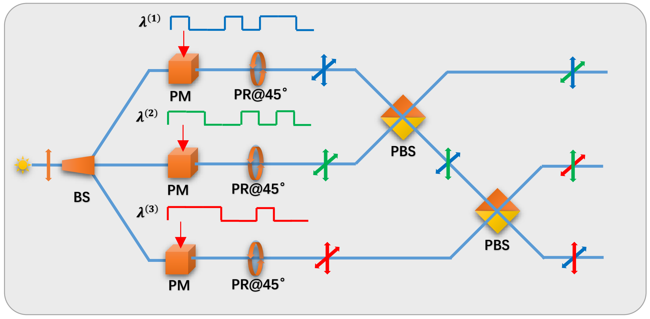
Figure 12: The scheme to realize the optical analogy to quantum GHZ state is shown, where PBS: polarization beam splitters, PR@$45^{\circ}$: $45^{\circ}$ polarization rotators.

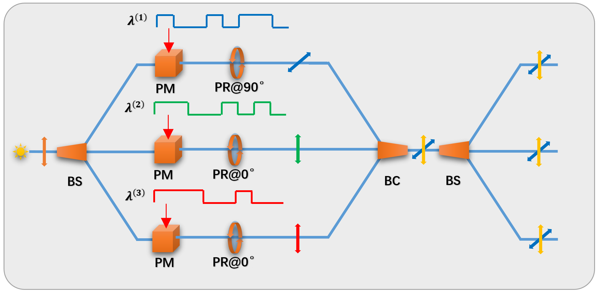
Figure 13: The sheme to realize the optical analogy to quantum W state is shown, where BC: beam couplers, BS: beam splitters, PR@$0^{\circ}$: $0^{\circ}$ polarization rotators, PR@$90^{\circ}$: $90^{\circ}$ polarization rotators.

Further, we make use of the coherent demodulation method mentioned in Section I to obtain the matrix $M$. Because each field of the imitations of GHZ state and W state has two orthogonal polarization modes, the coherent demodulation scheme need two LO fields with same orthogonal modes as the SO fields, as shown in Fig. 9. By using the software OPTISYSTEM, we construct the numerical simulation model as shown in Fig. 14 for the coherent demodulation as mensioned in Fig. 9. In Fig. 15, the electric signals of PDs are shown when the SO field is $E_{1}\left(t\right)$ of Eq. (105) and the LO fields are modulated with PPSs $\lambda^{\left(1\right)}$, $\lambda^{\left(2\right)}$, $\lambda^{\left(3\right)}$ respectively. Finally, by performing correlation analysis as mentioned in Section I.2, we can obtain the results for the three fields of Eq. (105), as shown in Fig. 16. After disposing of constant and normalization, we can express the measurement result as the matrix $M$ mentioned in Eq. (89). For the imitations of W state, the same results are shown in Fig. 17 and Fig. 18. After disposing of constant and normalization, we can also express the result as the matrix $M$ mentioned in Eq. (99).

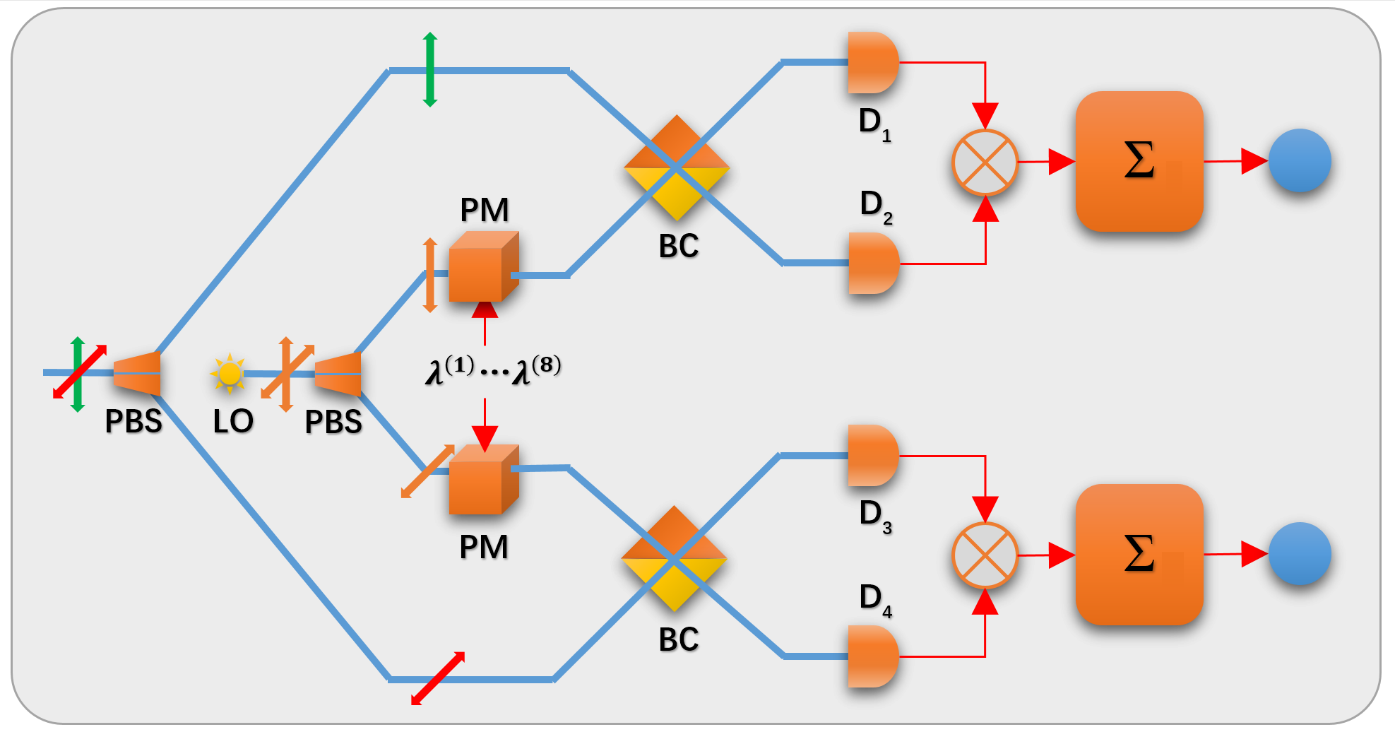
Figure 14: The numerical simulation model of the coherent demodulation as mentioned in Fig. 9 is shown, where PBS: polarization beam splitters and BC: beam couplers.

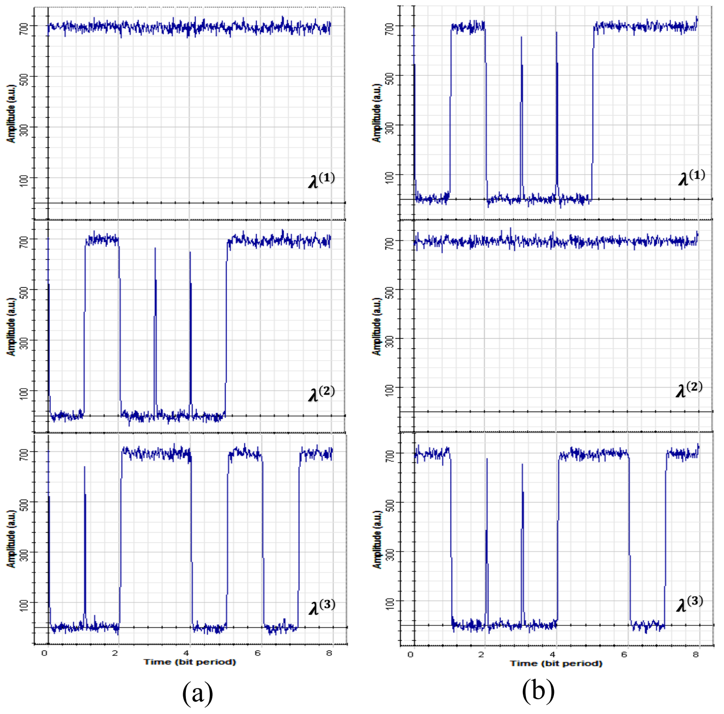
Figure 15: The electric signals for the field $E_{1}\left(t\right)$ of the GHZ imitation state with LO fields modulated with $\lambda^{\left(1\right)}$, $\lambda^{\left(2\right)}$ and $\lambda^{\left(3\right)}$ are shown, where (a) and (b) represent the two orthogonal modes $\left|0\right\rangle$ and $\left|1\right\rangle$ respectively.

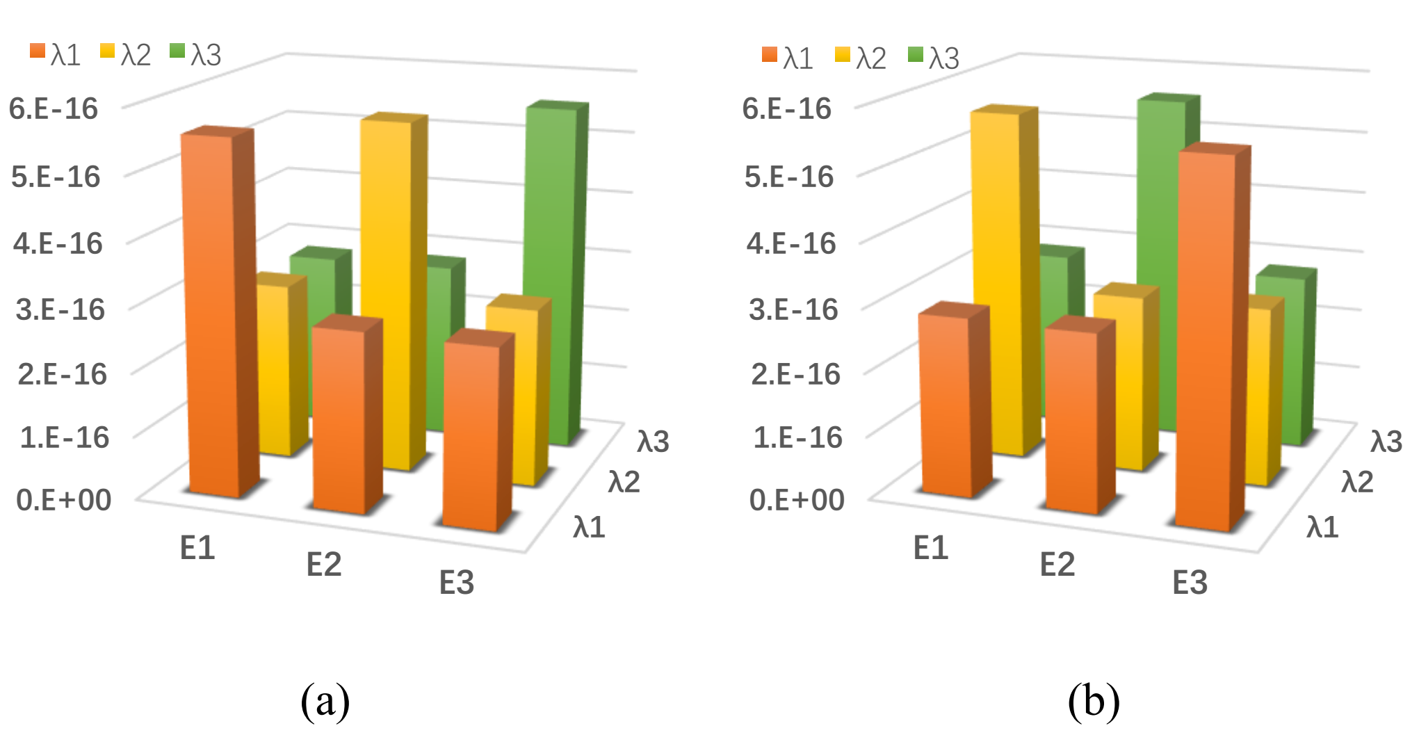
Figure 16: The correlation analysis results of GHZ state are shown, where (a) and (b) represent two orthogonal modes $A_{\uparrow}$ and $A_{\rightarrow}$ respectively, $E1$, $E2$, $E3$ three fields and $\lambda 1$, $\lambda 2$, $\lambda 3$ the sequences $\lambda^{\left(1\right)}$, $\lambda^{\left(2\right)}$, $\lambda^{\left(3\right)}$ modulating on LO.

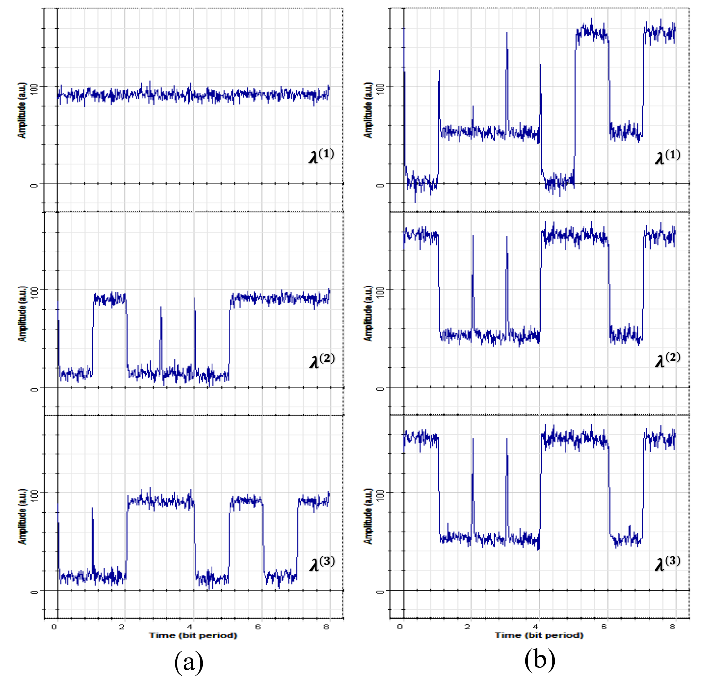
Figure 17: The electric signals for the field $E_{1}\left(t\right)$ of the W imitation state with LO fields modulated with $\lambda^{\left(1\right)}$, $\lambda^{\left(2\right)}$ and $\lambda^{\left(3\right)}$ are shown, where (a) and (b) represent two orthogonal modes $A_{\rightarrow}$ and $A_{\uparrow}$, respectively.

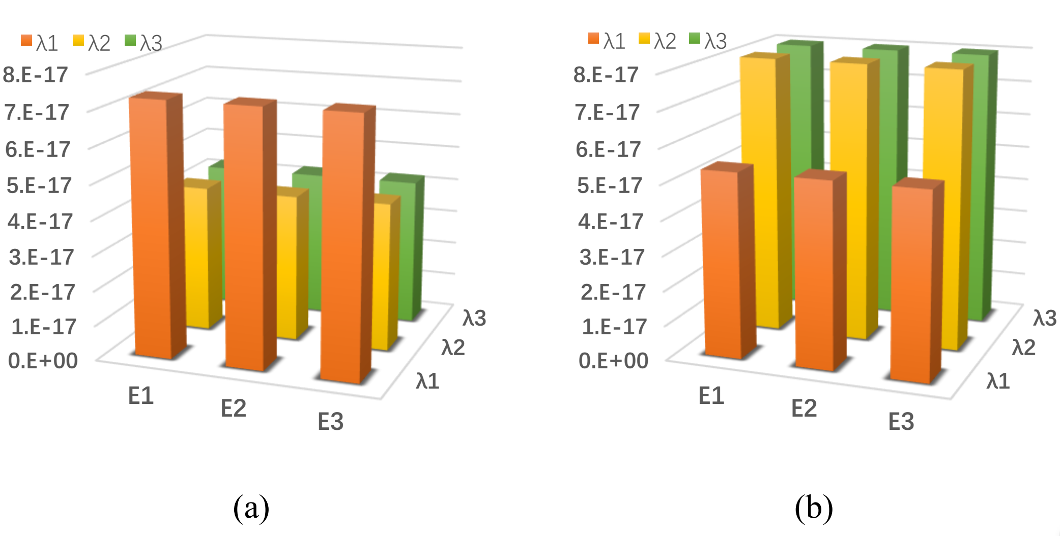
Figure 18: The correlation analysis results of W state are shown, where (a) and (b) represent two orthogonal modes $A_{\rightarrow}$ and $A_{\uparrow}$ respectively, $E1$, $E2$, $E3$ three fields and $\lambda 1$, $\lambda 2$, $\lambda 3$ the sequences $\lambda^{\left(1\right)}$, $\lambda^{\left(2\right)}$, $\lambda^{\left(3\right)}$ modulating on LO.

III Imitation of quantum computation

In this section, we will propose a gate array model to imitate quantum computation. In quantum computation, any quantum state can be obtained from an initial state by using a gate array constructed with universal CNOT gate and other single qubit gate Nielsen . Similarly, we can construct gate array models to produce the imitations of all kinds of quantum states, such as GHZ state and W state, even very sophisticated states like the results of Shor’s algorithm. We consider the gate array models can be employed as the imitations of quantum computation. Based on this understanding, we construct some gate array models to imitate Shor’s algorithm, Grover’s algorithm and quantum Fourier algorithm.

III.1 Gate array model to imitate quantum computation

In Ref. Fu1 , a constructure pathway of the imitation states is shown. Here we use the same model as shown Fig. 19, however the gate array model does not always achieve unitary transformations similar to quantum computation. Now we discuss some basic units of the gate array model besides the unitary transformation mensioned in Eq. (37) and the mode exchanger shown in Fig. 5.

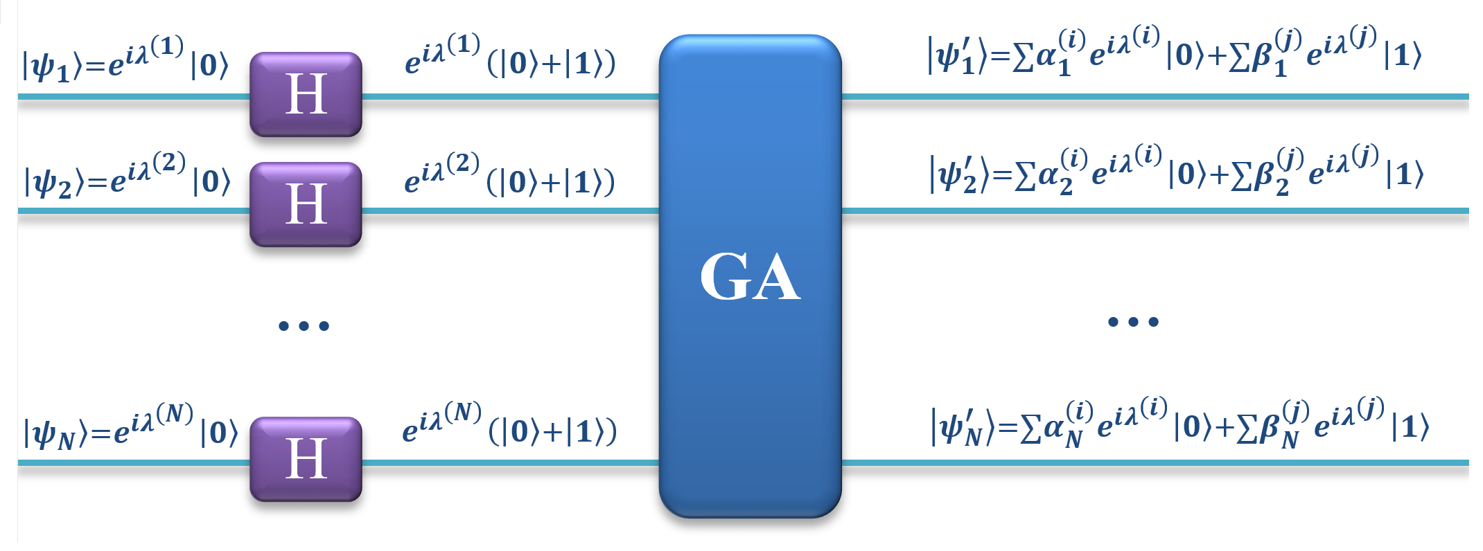
Figure 19: A GA model to imitate quantum computation is shown, where GA denotes the gate array.

(1) Combiner and splitter

Different from quantum state, we can conveniently combine and split an optical field by using an optical coupler/splitter device, which principles are discussed in Sec. I.3. The two basic devices are shown in Fig. 20 (a) and (b), respectively.

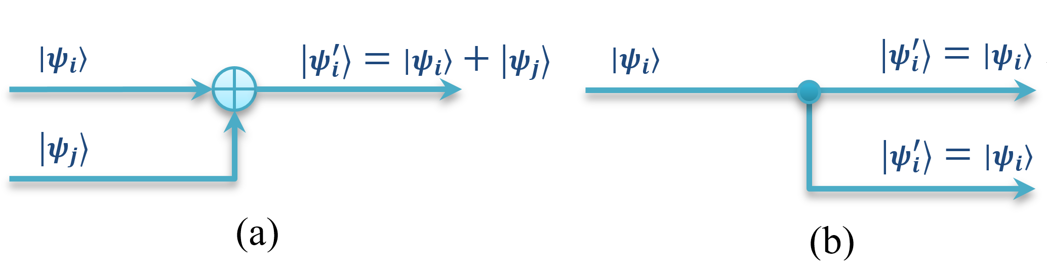
Figure 20: Two basic devices (a) coupler and (b) splitter are shown.

(b) Mode control gates

Further, we define $4$ kinds of mode control gates as selective mode transit devices with one input and one output as shown in Fig. 21. They are defined as follows

$$\mathbf{Gate\ }A : \left|\psi_{i}\right\rangle=e^{i\lambda^{\left(i\right)}}\left(\left|0\right\rangle+\left|1\right\rangle\right)\rightarrow\left|\psi_{i}^{\prime}\right\rangle=0,$$ (107)

$$\mathbf{Gate\ }B : \left|\psi_{i}\right\rangle=e^{i\lambda^{\left(i\right)}}\left(\left|0\right\rangle+\left|1\right\rangle\right)\rightarrow\left|\psi_{i}^{\prime}\right\rangle=e^{i\lambda^{\left(i\right)}}\left|0\right\rangle,$$

$$\mathbf{Gate\ }C : \left|\psi_{i}\right\rangle=e^{i\lambda^{\left(i\right)}}\left(\left|0\right\rangle+\left|1\right\rangle\right)\rightarrow\left|\psi_{i}^{\prime}\right\rangle=e^{i\lambda^{\left(i\right)}}\left|1\right\rangle,$$

$$\mathbf{Gate\ }D : \left|\psi_{i}\right\rangle=e^{i\lambda^{\left(i\right)}}\left(\left|0\right\rangle+\left|1\right\rangle\right)\rightarrow\left|\psi_{i}^{\prime}\right\rangle=e^{i\lambda^{\left(i\right)}}\left(\left|0\right\rangle+\left|1\right\rangle\right).$$

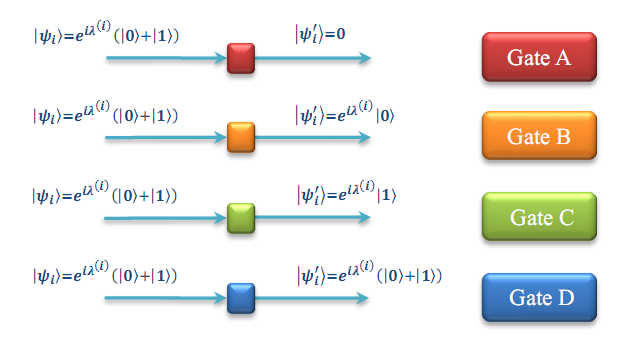
Figure 21: Mode control gates as selective mode transit devices are shown.

Now we discuss one of basic structures of gate array models. According to Sec. II, we can in principle imitate all quantum states by using the SCPM. Similar to field programmable gate array (FPGA), we propose a simple structure of gate array to satisfy the SCPM as shown in Fig. 22. Gate array $G_{kj}$ constituted by the basic units can transform $\left|\psi_{k}\right\rangle$ to achieve certain $\left|\psi_{k}^{\prime}\right\rangle$. It is easy to know that a sequence permutation with circulation of $p+1$ needs at least $p$ combiner devices and $2p$ control gates. We believe that many imitation states can be constructed by applying this structure that will be strictly proved in future paper.

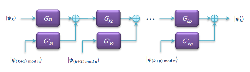
Figure 22: One of basic structrues of gate array model is shown.

Finally, we illustrate two gate array models to transform the product state to GHZ state and W state as shown in Fig. 23.

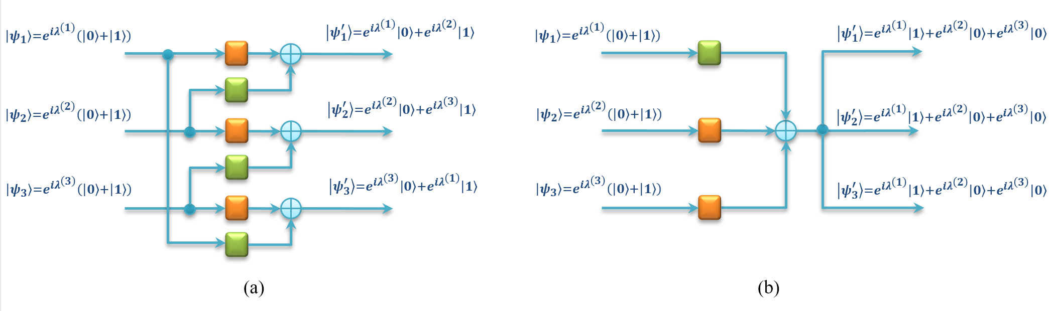
Figure 23: The gate array models to transform the product states to (a) GHZ state and (b) W state are shown.

III.2 Imitation of quantum algorithm

III.2.1 Analogy to Shor’s Algorithm

Shor’s algorithm is the most famous quantum algorithm for integer factorization that runs only in polynomial time on a quantum computer Shor . Specifically it takes time and quantum gates of order $O((\log L)^{2}(\log\log L)(\log\log\log L))$ using fast multiplication, demonstrating that the integer factorization problem can be efficiently solved on a quantum computer and is thus in the complexity class bounded error quantum polynomial time problem (BQP).

In this section, we propose a gate array model employing $8$ optical fields produces optical analogies that imitates the result state of Shor’s algorithm to factor $L=15$ into $3\times 5$. First, we chose a random number $a$ coprime with $15$, for example $a=7$. We define a function as follow

$$f\left(x\right)=a^{x}modL=7^{x}mod15.$$ (108)

The key step of the Shor’s algorithm is to obtain the period $r$ to satisfy

$$f\left(x+r\right)=7^{x+r}mod15=7^{x}mod15=f\left(x\right).$$ (109)

In order to construct $f\left(x\right)$, we prepare $8$ optical fields modulated with $8$ PPSs

$$\left|\psi_{n}\right\rangle=e^{i\lambda^{\left(n\right)}}\left(\left|0\right\rangle+\left|1\right\rangle\right),n=1\ldots 8.$$ (110)

We can express the product state as follows

$$\left|\Psi\right\rangle=\left|\psi_{1}\right\rangle\otimes\ldots\otimes\left|\psi_{8}\right\rangle=\sum\limits_{j=0}^{2^{8}-1}\left|j\right\rangle.$$ (111)

Further, we construct the gate array model as shown in Fig. 24. After passing through the gate array, the optical fields become the following forms

$$\left|\psi_{1}^{\prime}\right\rangle = \left(e^{i\lambda^{\left(1\right)}}+e^{i\lambda^{\left(2\right)}}+e^{i\lambda^{\left(3\right)}}+e^{i\lambda^{\left(4\right)}}\right)\left(\left|0\right\rangle+\left|1\right\rangle\right),$$ (112)

$$\left|\psi_{2}^{\prime}\right\rangle = \left(e^{i\lambda^{\left(2\right)}}+e^{i\lambda^{\left(3\right)}}+e^{i\lambda^{\left(4\right)}}+e^{i\lambda^{\left(5\right)}}\right)\left(\left|0\right\rangle+\left|1\right\rangle\right),$$

$$\left|\psi_{3}^{\prime}\right\rangle = \left(e^{i\lambda^{\left(3\right)}}+e^{i\lambda^{\left(4\right)}}\right)\left|0\right\rangle+\left(e^{i\lambda^{\left(5\right)}}+e^{i\lambda^{\left(6\right)}}\right)\left|1\right\rangle,$$

$$\left|\psi_{4}^{\prime}\right\rangle = \left(e^{i\lambda^{\left(4\right)}}+e^{i\lambda^{\left(6\right)}}\right)\left|0\right\rangle+\left(e^{i\lambda^{\left(5\right)}}+e^{i\lambda^{\left(7\right)}}\right)\left|1\right\rangle,$$

$$\left|\psi_{5}^{\prime}\right\rangle = \left(e^{i\lambda^{\left(5\right)}}+e^{i\lambda^{\left(6\right)}}+e^{i\lambda^{\left(7\right)}}\right)\left|0\right\rangle+e^{i\lambda^{\left(8\right)}}\left|1\right\rangle,$$

$$\left|\psi_{6}^{\prime}\right\rangle = e^{i\lambda^{\left(6\right)}}\left|0\right\rangle+\left(e^{i\lambda^{\left(7\right)}}+e^{i\lambda^{\left(8\right)}}+e^{i\lambda^{\left(1\right)}}\right)\left|1\right\rangle,$$

$$\left|\psi_{7}^{\prime}\right\rangle = \left(e^{i\lambda^{\left(7\right)}}+e^{i\lambda^{\left(1\right)}}+e^{i\lambda^{\left(2\right)}}\right)\left|0\right\rangle+e^{i\lambda^{\left(8\right)}}\left|1\right\rangle,$$

$$\left|\psi_{8}^{\prime}\right\rangle = e^{i\lambda^{\left(2\right)}}\left|0\right\rangle+\left(e^{i\lambda^{\left(8\right)}}+e^{i\lambda^{\left(1\right)}}+e^{i\lambda^{\left(3\right)}}\right)\left|1\right\rangle.$$

Using the coherent demodulation, we can obtain the matrix

$$M\left(\tilde{\alpha}_{i}^{j},\tilde{\beta}_{i}^{j}\right)=\left(\begin{array}[]{cccccccc}\left(1,1\right)&\left(1,1\right)&\left(1,1\right)&\left(1,1\right)&0&0&0&0\\ 0&\left(1,1\right)&\left(1,1\right)&\left(1,1\right)&\left(1,1\right)&0&0&0\\ 0&0&\left(1,0\right)&\left(1,0\right)&\left(0,1\right)&\left(0,1\right)&0&0\\ 0&0&0&\left(1,0\right)&\left(0,1\right)&\left(1,0\right)&\left(0,1\right)&0\\ 0&0&0&0&\left(1,0\right)&\left(1,0\right)&\left(1,0\right)&\left(0,1\right)\\ \left(0,1\right)&0&0&0&0&\left(1,0\right)&\left(0,1\right)&\left(0,1\right)\\ \left(1,0\right)&\left(1,0\right)&0&0&0&0&\left(1,0\right)&\left(0,1\right)\\ \left(0,1\right)&\left(1,0\right)&\left(0,1\right)&0&0&0&0&\left(0,1\right)\end{array}\right).$$ (113)

Using the scheme mentioned in Sec. II.3, we can obtain the imitated state

$$\left|\Psi^{\prime}\right\rangle = \left|7^{x}mod15\right\rangle\left|x\right\rangle=\left(\left|0\right\rangle+\left|4\right\rangle+\left|8\right\rangle+\left|12\right\rangle\right)\left|1\right\rangle$$

$$+\left(\left|1\right\rangle+\left|5\right\rangle+\left|9\right\rangle+\left|13\right\rangle\right)\left|7\right\rangle$$

$$+\left(\left|2\right\rangle+\left|6\right\rangle+\left|10\right\rangle+\left|14\right\rangle\right)\left|4\right\rangle$$

$$+\left(\left|3\right\rangle+\left|7\right\rangle+\left|11\right\rangle+\left|15\right\rangle\right)\left|13\right\rangle.$$

where the state $\left|7^{x}mod15\right\rangle$ is represented with the optical fields $\left|\psi_{1}^{\prime}\right\rangle\sim\left|\psi_{4}^{\prime}\right\rangle$ and $\left|x\right\rangle$ is represented with the optical fields $\left|\psi_{5}^{\prime}\right\rangle\sim\left|\psi_{8}^{\prime}\right\rangle$. There are four kinds of superposition classified from last four fields containing the values of $f\left(x\right)$ ($\left|1\right\rangle,\left|7\right\rangle,\left|4\right\rangle$ and $\left|13\right\rangle$) in the imitation state, which means the period of $f\left(x\right)=7^{x}mod15$ is $r=4$. It is worth noting that, different from quantum computing, we might obtain the expected period of without operating quantum Fourier transformation, at least for relatively small integer factorization. The remaining task is much easier. Because $L=15,a=7,r=4$, we obtain

$$\gcd\left(a^{\frac{r}{2}}\pm 1,L\right)=\gcd\left(7^{\frac{r}{2}}\pm 1,15\right)=\gcd\left(49\pm 1,15\right),$$ (115)

where $\gcd(48,15)=3$, and $\gcd(50,15)=5$. Finally, we can deduced that $L\left(15\right)=3\times 5$.

After further research the relation of the factorized integer and the gate array, we believe this might become a true scheme to imitate quantum Shor’s algorithm. Now the computation cost of the model is analyzed. The operation steps to get the imitation state include $3\times 8=24$ beam splitting operations, $6\times 8=48$ polarization mode operations, $3\times 8=24$ beam coupling operations. It can be seen that the number of operations is increased with the number of optical fields growth in linear growth. Considering each PPS has $8$ phase units, the total number of operations is proportional to $8^{2}$. In conclusion, it takes time and gates of order $O(\left(\log L\right)^{2})$.

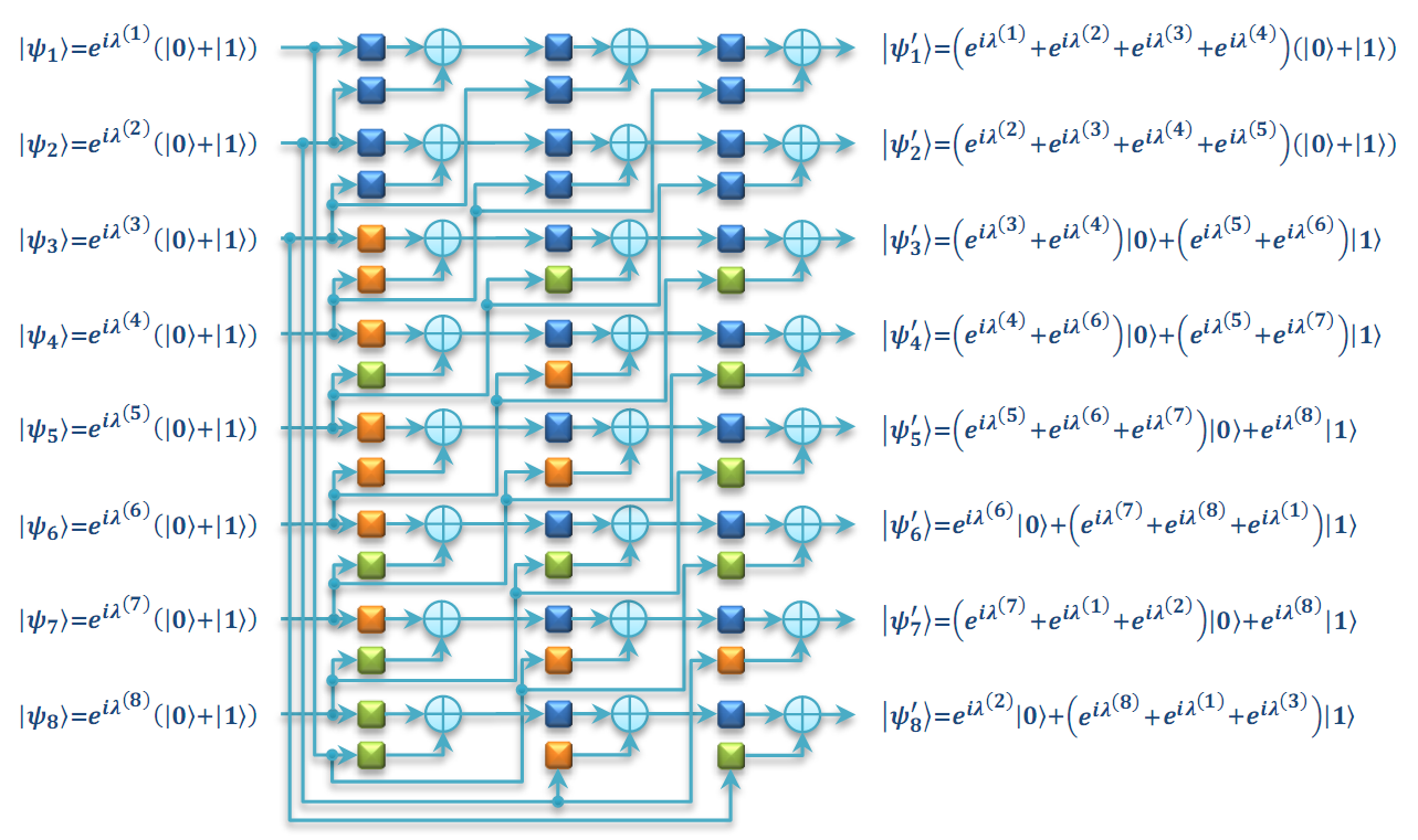
Figure 24: A gate array model to imitate Shor’s algorithm is shown.

III.2.2 Numerical simulation of the imitation

In this subsection, we discuss the numerical simulation of the gate model as shown Fig. 24 using the software OPTISYSTEM. The schematic diagram of numerical simulation is shown in Fig. 25. Firstly, the initial state can be prepared by the method as shown in Fig. 6, that is, modulate $8$ optical fields $E_{1}\sim E_{8}$ with $8$ PPSs respectively, and then rotate the polarization of each field by $45^{\circ}$ and evolve into the states in Eq. (110). After numerically simulating the complex gate array, we obtain the output fields and the electric signals of PDs after the interference between each fields and LO fields. Finally, the correlation results are obtained, substracted by the constant part and normalized, as shown in Fig. 26. After the threshold discrimination and binarization of results, we can express the measurement results as the $M$ matrix of Eq. (113) and the imitated state of Eq. (III.2.1). (Detailed the numerical calculus, derivation and OPTISYSTEM models will be provided in the supplementary materials). Using the SCPM mentioned in Sec. I.2, we can obtain the imitated state as shown Eq. (112).

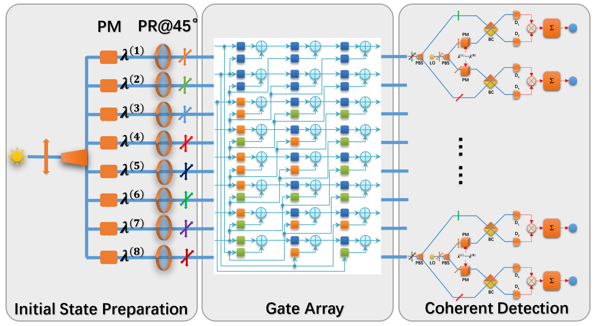
Figure 25: The numerical simulation scheme to factorized $15=3\times 5$ using the software OPTISYSTEM is shown.

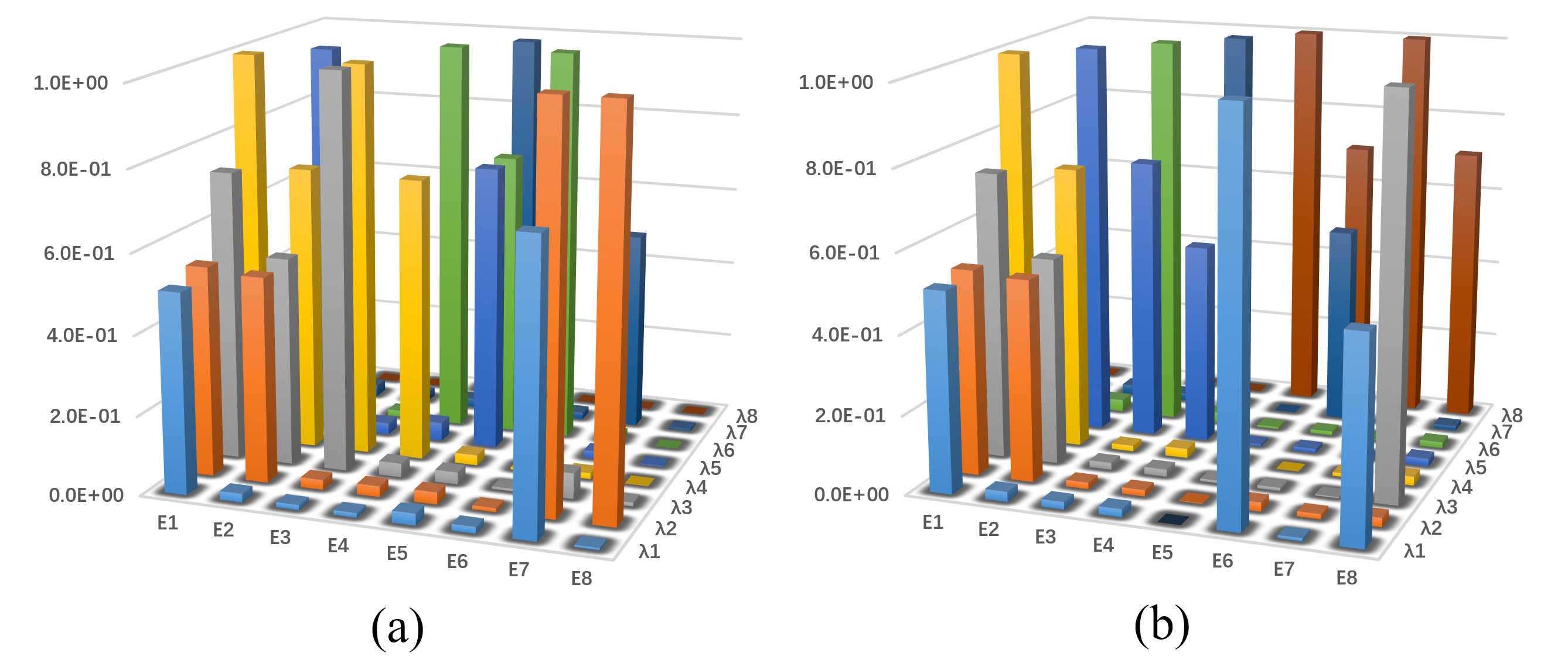
Figure 26: The correlation measurement results of the superposition state of the factorizing algorithm: (a) for mode $A_{\uparrow}$, and (b) for mode $A_{\rightarrow}$ are shown, where $E1\sim E8$ represent $\psi_{1}\sim\psi_{8}$ optical fields, and $\lambda 1\sim\lambda 8$ represent PPSs $\lambda^{\left(1\right)}\sim\lambda^{\left(8\right)}$.

III.2.3 Grover’s Algorithm

Grover’s algorithm is the quantum algorithm for searching an unsorted database with $2^{N}$ entries in $O(\sqrt{2^{N}})$ time and using $O(\log 2^{N})$ storage space Grover , that is faster than all classical computations. In fact its time complexity $O(\sqrt{2^{N}})$ is asymptotically the fastest possible for searching the unsorted database in the linear quantum model, however, it only provides a quadratic speedup rather than exponential speedup over their classical counterparts.

There are two key factors for searching an unsorted database: (1) to encode $2^{N}$ data into the superposition states of $N$ qubits and form a database; (2) to verify the existence of a specified number in the superposition states by measurements. In quantum computation, the first condition is very easy to be satisfied, but the second is difficult to achieve. Because the collapse of the superposition states to a specified state is completely uncontrollable in the quantum measurement. In Grover’s algorithm, the specified transformation is repeated to transform the superposition states for increasing the probability of the specified state, and after $O(\sqrt{2^{N}})$ repetitions the measuring probability will be close to $1/2$.

We now discuss the optical imitation of Grover’s algorithm. In our scheme, we can use $N$ optical fields modulated with PPSs. In principle, we can encode any $2^{N}$ data as the superposition state of $N$ optical fields to form a database. Different from the quantum computation, we can control the superposition state to output any specified state using a mode control gate array related to the specified state. Let $\left|S\right\rangle$ denote the superposition state of $N$ optical fields,

$$\left|S\right\rangle=\sum\limits_{i=1}^{2^{N}}\left|x_{i}\right\rangle,$$ (116)

where $\left|x_{i}\right\rangle$ can be encoded by any $2^{N}$ data. For example, we assume $\left|S\right\rangle$ as a superposition state of $13$ random numbers

$$\left|S\right\rangle = \left|59\right\rangle+\left|61\right\rangle+\left|63\right\rangle+\left|76\right\rangle+\left|117\right\rangle+\left|125\right\rangle+\left|140\right\rangle+\left|142\right\rangle+\left|148\right\rangle$$

$$+\left|187\right\rangle+\left|212\right\rangle+\left|238\right\rangle+\left|247\right\rangle$$

$$= \left|00111011\right\rangle+\left|00111101\right\rangle+\left|00111111\right\rangle+\left|01001100\right\rangle+\left|01110101\right\rangle$$

$$+\left|01111101\right\rangle+\left|10001100\right\rangle+\left|10001110\right\rangle+\left|10010100\right\rangle$$

$$+\left|10111011\right\rangle+\left|11010100\right\rangle+\left|11101110\right\rangle$$

$$+\left|11110111\right\rangle.$$

We choose $8$ optical fields modulated with $8$ PPSs and after passing through a suitable gate array, that become the following form

$$\left|\psi_{1}^{\prime}\right\rangle = \left(e^{i\lambda^{\left(1\right)}}+e^{i\lambda^{\left(2\right)}}+e^{i\lambda^{\left(5\right)}}+e^{i\lambda^{\left(8\right)}}\right)\left|0\right\rangle+\left(e^{i\lambda^{\left(3\right)}}+e^{i\lambda^{\left(4\right)}}+e^{i\lambda^{\left(5\right)}}+e^{i\lambda^{\left(6\right)}}+e^{i\lambda^{\left(7\right)}}\right)\left|1\right\rangle,$$ (118)

$$\left|\psi_{2}^{\prime}\right\rangle = \left(e^{i\lambda^{\left(2\right)}}+e^{i\lambda^{\left(4\right)}}+e^{i\lambda^{\left(5\right)}}+e^{i\lambda^{\left(6\right)}}\right)\left|0\right\rangle+\left(e^{i\lambda^{\left(1\right)}}+e^{i\lambda^{\left(3\right)}}+e^{i\lambda^{\left(5\right)}}+e^{i\lambda^{\left(7\right)}}+e^{i\lambda^{\left(8\right)}}\right)\left|1\right\rangle,$$

$$\left|\psi_{3}^{\prime}\right\rangle = \left(e^{i\lambda^{\left(2\right)}}+e^{i\lambda^{\left(5\right)}}+e^{i\lambda^{\left(6\right)}}\right)\left|0\right\rangle+\left(e^{i\lambda^{\left(1\right)}}+e^{i\lambda^{\left(3\right)}}+e^{i\lambda^{\left(4\right)}}+e^{i\lambda^{\left(7\right)}}+e^{i\lambda^{\left(8\right)}}\right)\left|1\right\rangle,$$

$$\left|\psi_{4}^{\prime}\right\rangle = \left(e^{i\lambda^{\left(1\right)}}+e^{i\lambda^{\left(3\right)}}+e^{i\lambda^{\left(6\right)}}+e^{i\lambda^{\left(8\right)}}\right)\left|0\right\rangle+\left(e^{i\lambda^{\left(2\right)}}+e^{i\lambda^{\left(4\right)}}+e^{i\lambda^{\left(5\right)}}+e^{i\lambda^{\left(7\right)}}\right)\left|1\right\rangle,$$

$$\left|\psi_{5}^{\prime}\right\rangle = \left(e^{i\lambda^{\left(3\right)}}+e^{i\lambda^{\left(6\right)}}+e^{i\lambda^{\left(8\right)}}\right)\left|0\right\rangle+\left(e^{i\lambda^{\left(1\right)}}+e^{i\lambda^{\left(2\right)}}+e^{i\lambda^{\left(4\right)}}+e^{i\lambda^{\left(5\right)}}+e^{i\lambda^{\left(6\right)}}+e^{i\lambda^{\left(7\right)}}\right)\left|1\right\rangle,$$

$$\left|\psi_{6}^{\prime}\right\rangle = e^{i\lambda^{\left(2\right)}}\left|0\right\rangle+\left(e^{i\lambda^{\left(1\right)}}+e^{i\lambda^{\left(3\right)}}+e^{i\lambda^{\left(4\right)}}+e^{i\lambda^{\left(5\right)}}+e^{i\lambda^{\left(6\right)}}+e^{i\lambda^{\left(7\right)}}+e^{i\lambda^{\left(8\right)}}\right)\left|1\right\rangle,$$

$$\left|\psi_{7}^{\prime}\right\rangle = \left(e^{i\lambda^{\left(1\right)}}+e^{i\lambda^{\left(2\right)}}+e^{i\lambda^{\left(6\right)}}+e^{i\lambda^{\left(7\right)}}+e^{i\lambda^{\left(8\right)}}\right)\left|0\right\rangle+\left(e^{i\lambda^{\left(1\right)}}+e^{i\lambda^{\left(3\right)}}+e^{i\lambda^{\left(4\right)}}+e^{i\lambda^{\left(5\right)}}+e^{i\lambda^{\left(7\right)}}\right)\left|1\right\rangle,$$

$$\left|\psi_{8}^{\prime}\right\rangle = \left(e^{i\lambda^{\left(2\right)}}+e^{i\lambda^{\left(3\right)}}+e^{i\lambda^{\left(5\right)}}+e^{i\lambda^{\left(7\right)}}\right)\left|0\right\rangle+\left(e^{i\lambda^{\left(1\right)}}+e^{i\lambda^{\left(4\right)}}+e^{i\lambda^{\left(6\right)}}+e^{i\lambda^{\left(8\right)}}\right)\left|1\right\rangle.$$

Due to the SCPM mentioned in Sec. II, any imitated state must correspond to a certain sequencial cycle permutation. Therefore, the problem to determine whether $\left|x\right\rangle$ exists in $\left|S\right\rangle$ become that to search the corresponding sequencial cycle permutation. For example, we search whether the number $\left|x\right\rangle=\left|148\right\rangle=\left|10010100\right\rangle$ is in $\left|S\right\rangle$. First, the optical fields of state $\left|S\right\rangle$ pass through the gate array controlled by $\left|x\right\rangle$ as shown in Fig. 27. Then we obtain the matrix $M$ by using the coherent demodulation

$$M\left(\tilde{\alpha}_{i}^{j},\tilde{\beta}_{i}^{j}\right)=\left(\begin{array}[]{cccccccc}0&0&\left(0,1\right)&\left(0,1\right)&\left(0,1\right)&\left(0,1\right)&\left(0,1\right)&0\\ 0&\left(1,0\right)&0&\left(1,0\right)&\left(1,0\right)&\left(1,0\right)&0&0\\ 0&\left(1,0\right)&0&0&\left(1,0\right)&\left(1,0\right)&0&0\\ 0&\left(0,1\right)&0&\left(0,1\right)&\left(0,1\right)&0&\left(0,1\right)&0\\ 0&0&\left(1,0\right)&0&0&\left(1,0\right)&0&\left(1,0\right)\\ \left(0,1\right)&0&\left(0,1\right)&\left(0,1\right)&\left(0,1\right)&\left(0,1\right)&\left(0,1\right)&\left(0,1\right)\\ \left(1,0\right)&\left(1,0\right)&0&0&0&\left(1,0\right)&\left(1,0\right)&\left(1,0\right)\\ 0&\left(1,0\right)&\left(1,0\right)&0&\left(1,0\right)&0&\left(1,0\right)&0\end{array}\right)$$ (119)

Finally, it is easy to search only the corresponding sequence permutation $R_{4}=\left\{\lambda^{\left(4\right)},\lambda^{\left(5\right)},\lambda^{\left(6\right)},\lambda^{\left(7\right)},\lambda^{\left(8\right)},\lambda^{\left(1\right)},\lambda^{\left(2\right)},\lambda^{\left(3\right)}\right\}$ within $O(N^{2})$ operation steps. If we choose $\left|x\right\rangle=\left|240\right\rangle=\left|11110000\right\rangle$, we can obtain the matrix

$$M\left(\tilde{\alpha}_{i}^{j},\tilde{\beta}_{i}^{j}\right)=\left(\begin{array}[]{cccccccc}0&0&\left(0,1\right)&\left(0,1\right)&\left(0,1\right)&\left(0,1\right)&\left(0,1\right)&0\\ \left(0,1\right)&0&\left(0,1\right)&0&\left(0,1\right)&0&\left(0,1\right)&\left(0,1\right)\\ \left(0,1\right)&0&\left(0,1\right)&\left(0,1\right)&0&0&\left(0,1\right)&\left(0,1\right)\\ 0&\left(0,1\right)&0&\left(0,1\right)&\left(0,1\right)&0&\left(0,1\right)&0\\ 0&0&\left(1,0\right)&0&0&\left(1,0\right)&0&\left(1,0\right)\\ 0&\left(1,0\right)&0&0&0&0&0&0\\ \left(1,0\right)&\left(1,0\right)&0&0&0&\left(1,0\right)&\left(1,0\right)&\left(1,0\right)\\ 0&\left(1,0\right)&\left(1,0\right)&0&\left(1,0\right)&0&\left(1,0\right)&0\end{array}\right).$$ (120)

In the matrix $M$, we can not search any corresponding sequencial cycle permutation. Therefore we can conclude $\left|x\right\rangle=\left|240\right\rangle$ does not exist in $\left|S\right\rangle$.

Different from Grover’s algorithm, this algorithm for searching an unsorted database with $2^{N}$ entries in $O(N^{2})$ operation steps and using $O(N^{2})$ storage space.

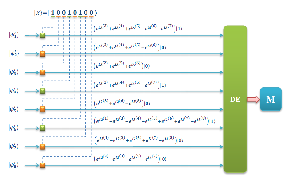
Figure 27: A gate array model to select $\left|x\right\rangle$ from $\left|S\right\rangle$ is shown.

III.3 Optical analogy to quantum Fourier algorithm

Quantum Fourier algorithm is one of the most important tools of quantum computation, and one of the algorithms which can bring about exponential speedup Nielsen . Shor’s algorithm, hidden subgroup problem and solving systems of linear equations make use of quantum Fourier algorithm Williams . Quantum Fourier algorithm utilizes the superposition of quantum state, whereby the required time and space for computation can be notably reduced from $2^{N}$ to $N$. Hence, the implementation of quantum Fourier algorithm is crucial to exponential speedup in quantum computation Deutsch . In this section, we first propose an optical Fourier algorithm to imitate quantum Fourier algorithm, then investigate the required computational resources, and at last demonstrate the algorithm applying to three optical fields as examples to verify its feasibility.

III.3.1 Quantum Fourier transform

Generally, quantum Fourier transform takes as input a vector of complex numbers, $f(0),f(1)\ldots,f(2^{N}-1)$, and output a new vector of complex numbers $\tilde{f}(0),\tilde{f}(1)\ldots,\tilde{f}(2^{N}-1)$ as follow

$$\tilde{f}\left(k\right)=\frac{1}{\sqrt{2^{N}}}\sum\limits_{j=0}^{2^{N}-1}e^{\frac{2\pi i}{2^{N}}jk}f\left(j\right).$$ (121)

This calculation involves the additions and multiplications of $2^{N}$ complex numbers, leading to an increase of computational complexity with the increase of the number of vector components. Classically, the most effective algorithm, fast Fourier transform is in time $O(2^{N}\log 2^{N})$. On the contrary, the quantum Fourier transform can be defined as a unitary transformation on $N$ qubits Nielsen , which is

$$\hat{F}\left|j\right\rangle=\frac{1}{\sqrt{2^{N}}}\sum\limits_{k=0}^{2^{N}-1}e^{\frac{2\pi i}{2^{N}}jk}\left|k\right\rangle.$$ (122)

Furthermore, the quantum Fourier transform of arbitrary state $\left|\Psi\right\rangle=C_{0}\left|0\right\rangle+\cdots+C_{2^{N}-1}\left|2^{N}-1\right\rangle$ can be expressed as

$$\left|\Psi\right\rangle_{F} \equiv \hat{F}\left|\Psi\right\rangle=C_{0}\hat{F}\left|0\right\rangle+C_{1}\hat{F}\left|1\right\rangle+\cdots+C_{2^{N}-1}\hat{F}\left|2^{N}-1\right\rangle$$

$$= \frac{1}{\sqrt{2^{N}}}\sum\limits_{k=0}^{2^{N}-1}\left[C_{0}\omega^{0\ast k}+C_{1}\omega^{1\ast k}+\cdots+C_{2^{N}-1}\omega^{\left(2^{N}-1\right)\ast k}\right]\left|k\right\rangle,$$

where $\omega=2\pi i/2^{N}$. Then, we expand $\left|\Psi\right\rangle_{F}$ into

$$\left|\Psi\right\rangle_{F}=\sum\limits_{j_{1}=0}^{1}\cdots\sum\limits_{j_{N}=0}^{1}D_{j_{N-1}\cdots j_{0}}\left|j_{N-1}\cdots j_{0}\right\rangle,$$ (124)

where the coefficients satisfy the following equation

$$\left(\begin{array}[]{c}D_{0}\\ D_{1}\\ \vdots\\ D_{2^{N}-1}\end{array}\right)=\frac{1}{\sqrt{2^{N}}}\left(\begin{array}[]{cccc}1&1&\cdots&1\\ 1&\omega&\cdots&\omega^{2^{N}-1}\\ \vdots&\vdots&\ddots&\vdots\\ 1&\omega^{2^{N}-1}&\cdots&\omega^{\left(2^{N}-1\right)^{2}}\end{array}\right)\left(\begin{array}[]{c}C_{0}\\ C_{1}\\ \vdots\\ C_{2^{N}-1}\end{array}\right).$$ (125)

In quantum Fourier transform, after the Hadamard gate and controlled-phase gate, we can obtain the final state $\left|j\right\rangle=\left|j_{N-1}j_{N-2}\cdots j_{0}\right\rangle$ of quantum Fourier transform

$$\hat{F}\left|j\right\rangle=\frac{1}{\sqrt{2^{N}}}\left(\left|1\right\rangle+e^{2\pi i0.j_{0}}\left|1\right\rangle\right)\left(\left|1\right\rangle+e^{2\pi i0.j_{1}j_{0}}\left|1\right\rangle\right)\cdots\left(\left|1\right\rangle+e^{2\pi i0.j_{N-1}j_{N-2}\cdots j_{0}}\left|1\right\rangle\right).$$ (126)

There are $N$ Hadamard gates and $N(N-1)/2$ controlled-phase gates on $N$ qubit registers, which means the quantum Fourier transform takes $O(N^{2})$ basic gate operations. Nevertheless, the quantum Fourier transform cannot output precise result of final states directly, but the probability of every state by repeated measurements, which can output the final result of Fourier transform at a certain accuracy Nielsen .

III.3.2 Algorithm for the optical analogies

As mentioned in Sec. II, a general form of $\left|\psi_{k}\right\rangle$ for $N$ fields can be constructed from Eq. (45) by using a gate array model,

$$\left|\psi_{n}\right\rangle = \sum\limits_{i=1}^{N}\alpha_{n}^{\left(i\right)}e^{i\lambda^{\left(i\right)}}\left|0\right\rangle+\sum\limits_{j=1}^{N}\beta_{n}^{\left(j\right)}e^{i\lambda^{\left(j\right)}}\left|1\right\rangle$$

$$\equiv \tilde{\alpha}_{n}\left|0\right\rangle+\tilde{\beta}_{n}\left|1\right\rangle,$$

where $\tilde{\alpha}_{n}\equiv\sum\limits_{i=1}^{N}\alpha_{n}^{\left(i\right)}e^{i\lambda^{\left(i\right)}},\tilde{\beta}_{n}\equiv\sum\limits_{j=1}^{N}\beta_{n}^{\left(j\right)}e^{i\lambda^{\left(j\right)}}$. Then, the formal product state Eq. (46) can be written as

$$\left|\Psi\right\rangle=\left(\tilde{\alpha}_{1}\left|0\right\rangle+\tilde{\beta}_{1}\left|1\right\rangle\right)\otimes\cdots\otimes\left(\tilde{\alpha}_{N}\left|0\right\rangle+\tilde{\beta}_{N}\left|1\right\rangle\right).$$ (128)

Further, we can obtain each item of the superposition of $\left|\Psi\right\rangle$ as follows

$$\begin{array}[]{c}C_{00\cdots 0}\left|00\cdots 0\right\rangle=\tilde{\alpha}_{1}\tilde{\alpha}_{2}\cdots\tilde{\alpha}_{N}\left|00\cdots 0\right\rangle,\\ C_{00\cdots 1}\left|00\cdots 1\right\rangle=\tilde{\alpha}_{1}\tilde{\alpha}_{2}\cdots\tilde{\beta}_{N}\left|00\cdots 1\right\rangle,\\ \vdots\\ C_{11\cdots 1}\left|11\cdots 1\right\rangle=\tilde{\beta}_{1}\tilde{\beta}_{2}\cdots\tilde{\beta}_{N}\left|11\cdots 1\right\rangle.\end{array}$$ (129)

The formal product state is expressed as follow

$$\left|\Psi\right\rangle=\sum\limits_{i_{1}=0}^{1}\cdots\sum\limits_{i_{N}=0}^{1}C_{i_{1}i_{2}\cdots i_{N}}\left|i_{1}i_{2}\cdots i_{N}\right\rangle.$$ (130)

After Fourier transform, this state evolves into

$$\left|\Psi\right\rangle_{F}=\hat{F}\left|\Psi\right\rangle,$$ (131)

where

$$\left|\Psi\right\rangle_{F}=\sum\limits_{j_{1}=0}^{1}\cdots\sum\limits_{j_{N}=0}^{1}D_{j_{1}j_{2}\cdots j_{N}}\left|j_{1}j_{2}\cdots j_{N}\right\rangle.$$ (132)

According to the definition Eq. (121), the relation between the coefficients $C_{i_{1}i_{2}\cdots i_{N}}$ and $D_{j_{1}j_{2}\cdots j_{N}}$ of these two states have to be satisfied as Eq. (125). To obtain the relation between these coefficient, we design the following algortithm:

(1) Selected a basis state $\left|j_{1}j_{2}\cdots j_{N}\right\rangle$ of $\left|\Psi\right\rangle_{F}$;

(2) Applying the following controlled-phase transformation on every field of $\left|\Psi\right\rangle$ according to the specific value of bits in the selected basis state, we obtain

$$\left\{\begin{array}[]{c}\left|\psi_{1}\right\rangle=\tilde{\alpha}_{1}\left|0\right\rangle+\tilde{\beta}_{1}\left|1\right\rangle\\ \left|\psi_{2}\right\rangle=\tilde{\alpha}_{2}\left|0\right\rangle+\omega^{j_{1}\ast 2^{N-2}}\tilde{\beta}_{2}\left|1\right\rangle\\ \left|\psi_{3}\right\rangle=\tilde{\alpha}_{3}\left|0\right\rangle+\omega^{j_{2}\ast 2^{N-2}+j_{1}\ast 2^{N-3}}\tilde{\beta}_{3}\left|1\right\rangle\\ \vdots\\ \left|\psi_{N}\right\rangle=\tilde{\alpha}_{N}\left|0\right\rangle+\omega^{j_{N-1}\ast 2^{N-2}+j_{N-2}\ast 2^{N-3}+\cdots+j_{1}\ast 1}\tilde{\beta}_{N}\left|1\right\rangle\end{array}\right.;$$ (133)

(3) Applying Hadamard gates on these fields, we obtain

$$\left\{\begin{array}[]{c}\left|\psi_{1}\right\rangle=\left(\tilde{\alpha}_{1}+\tilde{\beta}_{1}\right)\left|0\right\rangle+\left(\tilde{\alpha}_{1}-\tilde{\beta}_{1}\right)\left|1\right\rangle\\ \left|\psi_{2}\right\rangle=\left(\tilde{\alpha}_{2}+\omega^{j_{1}\ast 2^{N-2}}\tilde{\beta}_{2}\right)\left|0\right\rangle+\left(\tilde{\alpha}_{2}-\omega^{j_{1}\ast 2^{N-2}}\tilde{\beta}_{2}\right)\left|1\right\rangle\\ \left|\psi_{3}\right\rangle=\left(\tilde{\alpha}_{3}+\omega^{j_{2}\ast 2^{N-2}+j_{1}\ast 2^{N-3}}\tilde{\beta}_{3}\right)\left|0\right\rangle+\left(\tilde{\alpha}_{3}-\omega^{j_{2}\ast 2^{N-2}+j_{1}\ast 2^{N-3}}\tilde{\beta}_{3}\right)\left|1\right\rangle\\ \vdots\\ \left|\psi_{N}\right\rangle=\left(\tilde{\alpha}_{N}+\omega^{j_{N-1}\ast 2^{N-2}+j_{N-2}\ast 2^{N-3}+\cdots+j_{1}}\tilde{\beta}_{N}\right)\tilde{\alpha}_{N}\left|0\right\rangle+\left(\tilde{\alpha}_{N}-\omega^{j_{N-1}\ast 2^{N-2}+j_{N-2}\ast 2^{N-3}+\cdots+j_{1}}\tilde{\beta}_{N}\right)\left|1\right\rangle\end{array}\right.;$$ (134)

(4) Applying the mode control gates on these fields according to the specific values in $\left|j_{1}j_{2}\cdots j_{N}\right\rangle$, the mode of every field is identical to the corresponding value in $\left|j_{1}j_{2}\cdots j_{N}\right\rangle$, e.g., if $j_{1}=0$, $\left|\psi_{1}\right\rangle$ becomes$\ \left(\tilde{\alpha}_{1}+\tilde{\beta}_{1}\right)\left|0\right\rangle$, otherwise if $j_{1}=1$, $\left|\psi_{1}\right\rangle$ becomes$\ \left(\tilde{\alpha}_{1}-\tilde{\beta}_{1}\right)\left|1\right\rangle$, and so on;

(5) Applying the coherent demodulation on these fields and obtain the matrix $M$, we can obtain the corresponding coefficient $D_{j_{N}j_{N-1}\cdots j_{1}}$ using the method mentioned in Sec. II.3.

The above algorithm can be summarized as the following block diagram in Fig. 28. At last, we can analysis the computational complexity: there are $N$ optical fields in $\left|\Psi\right\rangle$ after $N$ controlled-phase gates, $N$ Hadamard gates, $N$ mode selection operations and finally $O\left(N^{2}\right)$ measurements in the coherent demodulation. Hence, the total number of operations is in $O(N^{2})$, which is the same as that in quantum Fourier algorithm. However, the result obtained in the optical algorithm is with certainty values but not with probability like quantum Fourier algorithm.

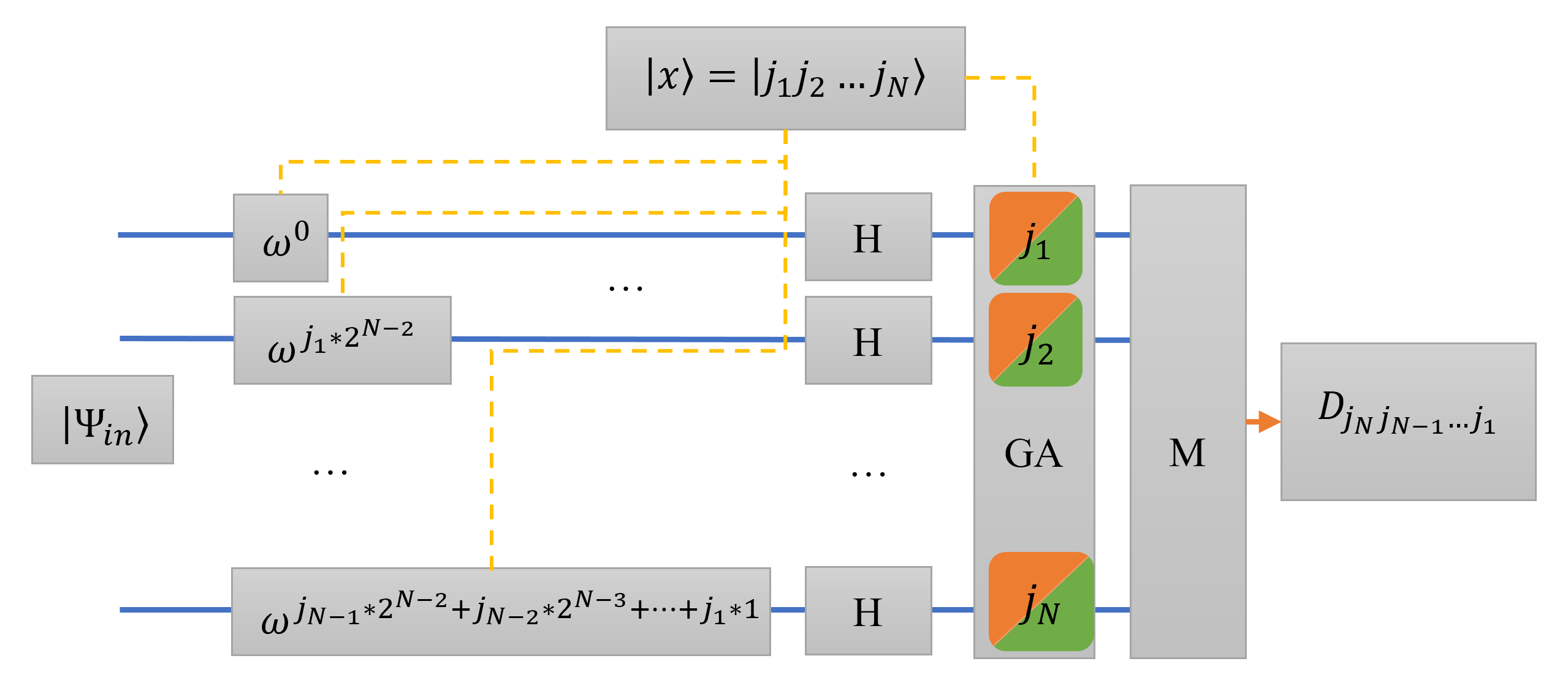
Figure 28: The algorithm diagram of optical analogy to quantum Fourier algorithm is shown.

III.3.3 The equivalence of ensemble-averaged states in optical algorithm

In the phase ensemble, we utilize the characteristic of PPS to define the EADM $\tilde{\rho}$ as mentioned in Sec. II.1.2. As mentioned in Sec. II.3, the imitation states can be constructured by using the SCPM corresponding to the minimum complete phase ensemble. Actually, the imitation states can be defined as the following ensemble-averaged state

$$\left|\tilde{\Psi}\right\rangle\equiv\sum\limits_{k=1}^{N}e^{-i\lambda^{S}}\left|\Psi\right\rangle,$$ (135)

where $\lambda^{S}=\sum\nolimits_{n=1}^{N}\lambda^{(n)}$ that is the sum of all used PPSs of the optical fields. Then, we discuss about Fourier transform for the ensemble-averaged states. From Eq. (125), we obtain the coefficients of Fourier transform satisfies

$$\begin{array}[]{c}D_{00\cdots 0}=C_{00\cdots 0}+C_{00\cdots 1}+\cdots+C_{11\cdots 1},\\ D_{00\cdots 1}=C_{00\cdots 0}+\omega C_{00\cdots 1}+\cdots+\omega^{\left(2^{N}-1\right)}C_{11\cdots 1},\\ \vdots\\ D_{11\cdots 0}=C_{00\cdots 0}+\omega^{\left(2^{N}-2\right)}C_{00\cdots 1}+\cdots+\omega^{\left(2^{N}-2\right)\left(2^{N}-1\right)}C_{11\cdots 1},\\ D_{11\cdots 1}=C_{00\cdots 0}+\omega^{\left(2^{N}-1\right)}C_{00\cdots 1}+\cdots+\omega^{\left(2^{N}-1\right)^{2}}C_{11\cdots 1}.\end{array}$$ (136)

In these equations, the combinations of $\omega$ and $C_{i_{1}i_{2}\cdots i_{N}}$ satisfy the following relations

$$\omega^{l}C_{i_{1}i_{2}\cdots i_{N}}=\sum\limits_{j=1}^{N}C_{i_{1}i_{2}\cdots i_{N}}^{\left(j\right)}e^{i\left[\lambda^{\left(j\right)}+\frac{2\pi l}{2^{N}}\right]}.$$ (137)

Obviously, these terms also satisfy the balance property of PPS. Hence, the ensemble-averaged state can also be used in Fourier transform. Then, we can obtain the Fourier transform

$$\left|\tilde{\Psi}\right\rangle_{F}\equiv\sum\limits_{k=1}^{N}e^{-i\lambda^{\left(S\right)}}\left|\Psi\right\rangle_{F}=\hat{F}\sum\limits_{k=1}^{N}e^{-i\lambda^{\left(S\right)}}\left|\Psi\right\rangle=\hat{F}\left|\tilde{\Psi}\right\rangle.$$ (138)

At last, we show the equivalence of ensemble-averaged states in the Fourier transform.

III.3.4 Optical analogies to quantum Fourier transform for three particles

According to Sec. II.3.1, three optical fields with PPSs $\lambda^{\left(i\right)}\left(i=1,2,3\right)$ are required to implement the imitations of the quantum states consisting of three particles. Modulated with these PPSs, three optical fields can be expressed as follows

$$\left\{\begin{array}[]{c}\left|\psi_{1}\right\rangle=e^{i\lambda^{\left(1\right)}}\left(\left|0\right\rangle+\left|1\right\rangle\right)\\ \left|\psi_{2}\right\rangle=e^{i\lambda^{\left(2\right)}}\left(\left|0\right\rangle+\left|1\right\rangle\right)\\ \left|\psi_{3}\right\rangle=e^{i\lambda^{\left(3\right)}}\left(\left|0\right\rangle+\left|1\right\rangle\right)\end{array}\right..$$ (139)

After gate array models as mentioned in Sec. III.1, we can obtain arbitrary quantum states which can be expressed as follows

$$\left\{\begin{array}[]{c}\left|\psi_{1}\right\rangle=\tilde{\alpha}_{1}\left|0\right\rangle+\tilde{\beta}_{1}\left|1\right\rangle\\ \left|\psi_{2}\right\rangle=\tilde{\alpha}_{2}\left|0\right\rangle+\tilde{\beta}_{2}\left|1\right\rangle\\ \left|\psi_{3}\right\rangle=\tilde{\alpha}_{3}\left|0\right\rangle+\tilde{\beta}_{3}\left|1\right\rangle\end{array}\right..$$ (140)

According to the algorithm in Sec. III.3.2, we obtain:

(1) Apply controlled-phase gates on three optical fields respectively

$$\left\{\begin{array}[]{c}\left|\psi_{1}\right\rangle=\tilde{\alpha}_{1}\left|0\right\rangle+\tilde{\beta}_{1}\left|1\right\rangle\\ \left|\psi_{2}\right\rangle=\tilde{\alpha}_{2}\left|0\right\rangle+\omega^{j_{1}\ast 2}\tilde{\beta}_{2}\left|1\right\rangle\\ \left|\psi_{3}\right\rangle=\tilde{\alpha}_{3}\left|0\right\rangle+\omega^{j_{2}\ast 2+j_{1}\ast 1}\tilde{\beta}_{3}\left|1\right\rangle\end{array}\right..$$ (141)

where $\omega=e^{2\pi i/8}$.

(2) Hadamard transformation

$$\left\{\begin{array}[]{c}\left|\psi_{1}\right\rangle=\left(\tilde{\alpha}_{1}+\tilde{\beta}_{1}\right)\left|0\right\rangle+\left(\tilde{\alpha}_{1}-\tilde{\beta}_{1}\right)\left|1\right\rangle\\ \left|\psi_{2}\right\rangle=\left(\tilde{\alpha}_{2}+\omega^{j_{1}\ast 2}\tilde{\beta}_{2}\right)\left|0\right\rangle+\left(\tilde{\alpha}_{2}-\omega^{j_{1}\ast 2}\tilde{\beta}_{2}\right)\left|1\right\rangle\\ \left|\psi_{3}\right\rangle=\left(\tilde{\alpha}_{3}+\omega^{j_{2}\ast 2+j_{1}\ast 1}\tilde{\beta}_{3}\right)\left|0\right\rangle+\left(\tilde{\alpha}_{3}-\omega^{j_{2}\ast 2+j_{1}\ast 1}\tilde{\beta}_{3}\right)\left|1\right\rangle\end{array}\right..$$ (142)

(3) Calculate coefficients

(3.1) When $\left|j_{1}j_{2}j_{3}\right\rangle=\left|000\right\rangle$ and $\left|j_{1}j_{2}j_{3}\right\rangle=\left|001\right\rangle$,

$$\left\{\begin{array}[]{c}\left|\psi_{1}\right\rangle=\tilde{\alpha}_{1}\left|0\right\rangle+\tilde{\beta}_{1}\left|1\right\rangle\\ \left|\psi_{2}\right\rangle=\tilde{\alpha}_{2}\left|0\right\rangle+\omega^{0\ast 2}\tilde{\beta}_{2}\left|1\right\rangle\\ \left|\psi_{3}\right\rangle=\tilde{\alpha}_{3}\left|0\right\rangle+\omega^{0\ast 2+0\ast 1}\tilde{\beta}_{3}\left|1\right\rangle\end{array}\right.\rightarrow\left\{\begin{array}[]{c}\left|\psi_{1}\right\rangle=\left(\tilde{\alpha}_{1}+\tilde{\beta}_{1}\right)\left|0\right\rangle+\left(\tilde{\alpha}_{1}-\tilde{\beta}_{1}\right)\left|1\right\rangle\\ \left|\psi_{2}\right\rangle=\left(\tilde{\alpha}_{2}+\tilde{\beta}_{2}\right)\left|0\right\rangle+\left(\tilde{\alpha}_{2}-\tilde{\beta}_{2}\right)\left|1\right\rangle\\ \left|\psi_{3}\right\rangle=\left(\tilde{\alpha}_{3}+\tilde{\beta}_{3}\right)\left|0\right\rangle+\left(\tilde{\alpha}_{3}-\tilde{\beta}_{3}\right)\left|1\right\rangle\end{array}\right..$$ (143)

Then we obtain the corresponding coefficients $D_{000}$ and $D_{100}$

$$D_{000} = \left(\tilde{\alpha}_{1}+\tilde{\beta}_{1}\right)\left(\tilde{\alpha}_{2}+\tilde{\beta}_{2}\right)\left(\tilde{\alpha}_{3}+\tilde{\beta}_{3}\right)$$

$$= C_{000}+C_{001}+C_{010}+C_{011}+C_{100}+C_{101}+C_{110}+C_{111},$$

$$D_{100} = \left(\tilde{\alpha}_{1}+\tilde{\beta}_{1}\right)\left(\tilde{\alpha}_{2}+\tilde{\beta}_{2}\right)\left(\tilde{\alpha}_{3}-\tilde{\beta}_{3}\right)$$

$$= C_{000}-C_{001}+C_{010}-C_{011}+C_{100}-C_{101}+C_{110}-C_{111}.$$

(3.2) When $\left|j_{1}j_{2}j_{3}\right\rangle=\left|010\right\rangle$ and $\left|j_{1}j_{2}j_{3}\right\rangle=\left|011\right\rangle$,

$$\left\{\begin{array}[]{c}\left|\psi_{1}\right\rangle=\tilde{\alpha}_{1}\left|0\right\rangle+\tilde{\beta}_{1}\left|1\right\rangle\\ \left|\psi_{2}\right\rangle=\tilde{\alpha}_{2}\left|0\right\rangle+\omega^{0\ast 2}\tilde{\beta}_{2}\left|1\right\rangle\\ \left|\psi_{3}\right\rangle=\tilde{\alpha}_{3}\left|0\right\rangle+\omega^{1\ast 2+0\ast 1}\tilde{\beta}_{3}\left|1\right\rangle\end{array}\right.\rightarrow\left\{\begin{array}[]{c}\left|\psi_{1}\right\rangle=\left(\tilde{\alpha}_{1}+\tilde{\beta}_{1}\right)\left|0\right\rangle+\left(\tilde{\alpha}_{1}-\tilde{\beta}_{1}\right)\left|1\right\rangle\\ \left|\psi_{2}\right\rangle=\left(\tilde{\alpha}_{2}+\tilde{\beta}_{2}\right)\left|0\right\rangle+\left(\tilde{\alpha}_{2}-\tilde{\beta}_{2}\right)\left|1\right\rangle\\ \left|\psi_{3}\right\rangle=\left(\tilde{\alpha}_{3}+\omega^{2}\tilde{\beta}_{3}\right)\left|0\right\rangle+\left(\tilde{\alpha}_{3}-\omega^{2}\tilde{\beta}_{3}\right)\left|1\right\rangle\end{array}\right..$$ (146)

Then we obtain the corresponding coefficients $D_{010}$ and $D_{110}$

$$D_{010} = \left(\tilde{\alpha}_{1}+\tilde{\beta}_{1}\right)\left(\tilde{\alpha}_{2}-\tilde{\beta}_{2}\right)\left(\tilde{\alpha}_{3}+\omega^{2}\tilde{\beta}_{3}\right)$$

$$= C_{000}+\omega^{2}C_{001}-C_{010}-\omega^{2}C_{011}+C_{100}+\omega^{2}C_{101}-C_{110}-\omega^{2}C_{111},$$

$$D_{110} = \left(\tilde{\alpha}_{1}+\tilde{\beta}_{1}\right)\left(\tilde{\alpha}_{2}-\tilde{\beta}_{2}\right)\left(\tilde{\alpha}_{3}-\omega^{2}\tilde{\beta}_{3}\right)$$

$$= C_{000}-\omega^{2}C_{001}-C_{010}+\omega^{2}C_{011}+C_{100}-\omega^{2}C_{101}-C_{110}+\omega^{2}C_{111}.$$

(3.3) When $\left|j_{1}j_{2}j_{3}\right\rangle=\left|100\right\rangle$ and $\left|j_{1}j_{2}j_{3}\right\rangle=\left|101\right\rangle$,

$$\left\{\begin{array}[]{c}\left|\psi_{1}\right\rangle=\tilde{\alpha}_{1}\left|0\right\rangle+\tilde{\beta}_{1}\left|1\right\rangle\\ \left|\psi_{2}\right\rangle=\tilde{\alpha}_{2}\left|0\right\rangle+\omega^{1\ast 2}\tilde{\beta}_{2}\left|1\right\rangle\\ \left|\psi_{3}\right\rangle=\tilde{\alpha}_{3}\left|0\right\rangle+\omega^{0\ast 2+1\ast 1}\tilde{\beta}_{3}\left|1\right\rangle\end{array}\right.\rightarrow\left\{\begin{array}[]{c}\left|\psi_{1}\right\rangle=\left(\tilde{\alpha}_{1}+\tilde{\beta}_{1}\right)\left|0\right\rangle+\left(\tilde{\alpha}_{1}-\tilde{\beta}_{1}\right)\left|1\right\rangle\\ \left|\psi_{2}\right\rangle=\left(\tilde{\alpha}_{2}+\omega^{2}\tilde{\beta}_{2}\right)\left|0\right\rangle+\left(\tilde{\alpha}_{2}-\omega^{2}\tilde{\beta}_{2}\right)\left|1\right\rangle\\ \left|\psi_{3}\right\rangle=\left(\tilde{\alpha}_{3}+\omega\tilde{\beta}_{3}\right)\left|0\right\rangle+\left(\tilde{\alpha}_{3}-\omega\tilde{\beta}_{3}\right)\left|1\right\rangle\end{array}\right..$$ (149)

Then we obtain the corresponding coefficients $D_{001}$ and $D_{101}$

$$D_{001} = \left(\tilde{\alpha}_{1}-\tilde{\beta}_{1}\right)\left(\tilde{\alpha}_{2}+\omega^{2}\tilde{\beta}_{2}\right)\left(\tilde{\alpha}_{3}+\omega\tilde{\beta}_{3}\right)$$

$$= C_{000}+\omega C_{001}+\omega^{2}C_{010}+\omega^{3}C_{011}-C_{100}-\omega C_{101}-\omega^{2}C_{110}-\omega^{3}C_{111},$$

$$D_{101} = \left(\tilde{\alpha}_{1}-\tilde{\beta}_{1}\right)\left(\tilde{\alpha}_{2}+\omega^{2}\tilde{\beta}_{2}\right)\left(\tilde{\alpha}_{3}-\omega\tilde{\beta}_{3}\right)$$

$$= C_{000}-\omega C_{001}+\omega^{2}C_{010}-\omega^{3}C_{011}-C_{100}+\omega C_{101}-\omega^{2}C_{110}+\omega^{3}C_{111}.$$

(3.4) When $\left|j_{1}j_{2}j_{3}\right\rangle=\left|110\right\rangle$ and $\left|j_{1}j_{2}j_{3}\right\rangle=\left|111\right\rangle$,

$$\left\{\begin{array}[]{c}\left|\psi_{1}\right\rangle=\tilde{\alpha}_{1}\left|0\right\rangle+\tilde{\beta}_{1}\left|1\right\rangle\\ \left|\psi_{2}\right\rangle=\tilde{\alpha}_{2}\left|0\right\rangle+\omega^{1\ast 2}\tilde{\beta}_{2}\left|1\right\rangle\\ \left|\psi_{3}\right\rangle=\tilde{\alpha}_{3}\left|0\right\rangle+\omega^{1\ast 2+1\ast 1}\tilde{\beta}_{3}\left|1\right\rangle\end{array}\right.\rightarrow\left\{\begin{array}[]{c}\left|\psi_{1}\right\rangle=\left(\tilde{\alpha}_{1}+\tilde{\beta}_{1}\right)\left|0\right\rangle+\left(\tilde{\alpha}_{1}-\tilde{\beta}_{1}\right)\left|1\right\rangle\\ \left|\psi_{2}\right\rangle=\left(\tilde{\alpha}_{2}+\omega^{2}\tilde{\beta}_{2}\right)\left|0\right\rangle+\left(\tilde{\alpha}_{2}-\omega^{2}\tilde{\beta}_{2}\right)\left|1\right\rangle\\ \left|\psi_{3}\right\rangle=\left(\tilde{\alpha}_{3}+\omega^{3}\tilde{\beta}_{3}\right)\left|0\right\rangle+\left(\tilde{\alpha}_{3}-\omega^{3}\tilde{\beta}_{3}\right)\left|1\right\rangle\end{array}\right..$$ (152)

Then we obtain the corresponding coefficients $D_{011}$ and $D_{111}$

$$D_{011} = \left(\tilde{\alpha}_{1}-\tilde{\beta}_{1}\right)\left(\tilde{\alpha}_{2}-\omega^{2}\tilde{\beta}_{2}\right)\left(\tilde{\alpha}_{3}+\omega^{3}\tilde{\beta}_{3}\right)$$

$$= C_{000}+\omega^{3}C_{001}-\omega^{2}C_{010}-\omega^{5}C_{011}-C_{100}-\omega^{3}C_{101}+\omega^{2}C_{110}+\omega^{5}C_{111},$$

$$D_{111} = \left(\tilde{\alpha}_{1}-\tilde{\beta}_{1}\right)\left(\tilde{\alpha}_{2}-\tilde{\beta}_{2}\right)\left(\tilde{\alpha}_{3}-\omega^{2}\tilde{\beta}_{3}\right)$$

$$= C_{000}-\omega^{3}C_{001}-\omega^{2}C_{010}+\omega^{5}C_{011}-C_{100}+\omega^{3}C_{101}+\omega^{2}C_{110}-\omega^{5}C_{111}.$$

At last, we obtain the transform matrix of all coefficients as follow

$$\left(\begin{array}[]{c}D_{000}\\ D_{001}\\ D_{010}\\ D_{011}\\ D_{100}\\ D_{101}\\ D_{110}\\ D_{111}\end{array}\right)=\left(\begin{array}[]{cccccccc}1&1&1&1&1&1&1&1\\ 1&\omega&\omega^{2}&\omega^{3}&-1&-\omega&-\omega^{2}&-\omega^{3}\\ 1&\omega^{2}&-1&-\omega^{2}&1&\omega^{2}&-1&\omega^{2}\\ 1&\omega^{3}&-\omega^{2}&\omega&-1&-\omega^{3}&\omega^{2}&-\omega\\ 1&-1&1&-1&1&-1&1&-1\\ 1&-\omega&\omega^{2}&-\omega^{3}&-1&\omega&-\omega^{2}&\omega^{3}\\ 1&-\omega^{2}&-1&\omega^{2}&1&-\omega^{2}&-1&\omega^{2}\\ 1&-\omega^{3}&-\omega^{2}&-\omega&-1&\omega^{3}&\omega^{2}&\omega\end{array}\right)\left(\begin{array}[]{c}C_{000}\\ C_{001}\\ C_{010}\\ C_{011}\\ C_{100}\\ C_{101}\\ C_{110}\\ C_{111}\end{array}\right).$$ (155)

Obviously, the result is completely similar to quantum Fourier algorithm. We will utilize the above algorithm applying to some imitation states of three optical fields as following examples:

(1) the product state

In quantum mechanics, the product state of three particles is $\left|\Psi\right\rangle=\frac{1}{\sqrt{8}}\left(\left|000\right\rangle+\left|001\right\rangle+\cdots+\left|111\right\rangle\right)$. We can expressed three fields as Eq. (139), except for normalization constant. According to the definition of the ensemble-averaged state Eq. (135), we obtain the imitation state

$$\left|\tilde{\Psi}\right\rangle=\left|000\right\rangle+\left|001\right\rangle+\cdots+\left|111\right\rangle.$$ (156)

Using the above algorithm, we can easily obtain the Fourier transform coefficients $D_{000}=C_{000}+C_{001}+\cdots+C_{111}=8e^{i\left(\lambda^{\left(1\right)}+\lambda^{\left(2\right)}+\lambda^{\left(3\right)}\right)}$, while the other terms is $0$. Then we obtain the ensemble-averaged state

$$\left|\tilde{\Psi}\right\rangle_{F}=8\left|000\right\rangle,$$ (157)

which is identical to quantum Fourier transform, except for the normalization constant.

(2) GHZ state

In quantum mechanics, GHZ state is the biggest entanglement state of three particles. According to Sec. II.3.1, we can obtain the following form of three optical fields

$$\left\{\begin{array}[]{c}\left|\psi_{1}\right\rangle=\tilde{\alpha}_{1}\left|0\right\rangle+\tilde{\beta}_{1}\left|1\right\rangle=e^{i\lambda^{\left(1\right)}}\left|0\right\rangle+e^{i\lambda^{\left(2\right)}}\left|1\right\rangle\\ \left|\psi_{2}\right\rangle=\tilde{\alpha}_{2}\left|0\right\rangle+\tilde{\beta}_{2}\left|1\right\rangle=e^{i\lambda^{\left(2\right)}}\left|0\right\rangle+e^{i\lambda^{\left(3\right)}}\left|1\right\rangle\\ \left|\psi_{3}\right\rangle=\tilde{\alpha}_{3}\left|0\right\rangle+\tilde{\beta}_{3}\left|1\right\rangle=e^{i\lambda^{\left(3\right)}}\left|0\right\rangle+e^{i\lambda^{\left(1\right)}}\left|1\right\rangle\end{array}\right..$$ (158)

The formal product state can be expressed as

$$\left|\Psi\right\rangle = \left|\psi_{1}\right\rangle\otimes\left|\psi_{2}\right\rangle\otimes\left|\psi_{3}\right\rangle=e^{i\left(\lambda^{\left(1\right)}+\lambda^{\left(2\right)}+\lambda^{\left(3\right)}\right)}\left[\left|000\right\rangle+\left|111\right\rangle+e^{i\left(\lambda^{\left(1\right)}-\lambda^{\left(3\right)}\right)}\left|001\right\rangle\right.$$

$$+e^{i\left(\lambda^{\left(3\right)}-\lambda^{\left(2\right)}\right)}\left|010\right\rangle+e^{i\left(\lambda^{\left(1\right)}-\lambda^{\left(2\right)}\right)}\left|011\right\rangle+e^{i\left(\lambda^{\left(2\right)}-\lambda^{\left(1\right)}\right)}\left|100\right\rangle$$

$$\left.+e^{i\left(\lambda^{\left(2\right)}-\lambda^{\left(3\right)}\right)}\left|101\right\rangle+e^{i\left(\lambda^{\left(3\right)}-\lambda^{\left(1\right)}\right)}\left|110\right\rangle\right].$$

According to the definition Eq. (135), we obtain the ensemble-averaged state

$$\left|\tilde{\Psi}\right\rangle=\left|000\right\rangle+\left|111\right\rangle.$$ (160)

Similarly, except for normalization constant and overall phase factor, the state is identical to GHZ state. Using the above algorithm, we can easily obtain the Fourier transform coefficients as follows

$$D_{000} = \left(\tilde{\alpha}_{1}+\tilde{\beta}_{1}\right)\left(\tilde{\alpha}_{2}+\tilde{\beta}_{2}\right)\left(\tilde{\alpha}_{3}+\tilde{\beta}_{3}\right)=2e^{i\left(\lambda^{\left(1\right)}+\lambda^{\left(2\right)}+\lambda^{\left(3\right)}\right)}+e^{i\left(2\lambda^{\left(1\right)}+\lambda^{\left(2\right)}\right)}+e^{i\left(2\lambda^{\left(1\right)}+\lambda^{\left(3\right)}\right)}$$

$$+e^{i\left(2\lambda^{\left(2\right)}+\lambda^{\left(1\right)}\right)}+e^{i\left(2\lambda^{\left(2\right)}+\lambda^{\left(3\right)}\right)}+e^{i\left(2\lambda^{\left(3\right)}+\lambda^{\left(1\right)}\right)}+e^{i\left(2\lambda^{\left(3\right)}+\lambda^{\left(2\right)}\right)},$$

$$D_{001} = \left(\tilde{\alpha}_{1}-\tilde{\beta}_{1}\right)\left(\tilde{\alpha}_{2}+\omega^{2}\tilde{\beta}_{2}\right)\left(\tilde{\alpha}_{3}+\omega\tilde{\beta}_{3}\right)=\left(1-\omega^{3}\right)e^{i\left(\lambda^{\left(1\right)}+\lambda^{\left(2\right)}+\lambda^{\left(3\right)}\right)}+\omega e^{i\left(2\lambda^{\left(1\right)}+\lambda^{\left(2\right)}\right)}$$

$$+\omega^{3}e^{i\left(2\lambda^{\left(1\right)}+\lambda^{\left(3\right)}\right)}-\omega e^{i\left(2\lambda^{\left(2\right)}+\lambda^{\left(1\right)}\right)}-e^{i\left(2\lambda^{\left(2\right)}+\lambda^{\left(3\right)}\right)}+\omega^{2}e^{i\left(2\lambda^{\left(3\right)}+\lambda^{\left(1\right)}\right)}$$

$$-\omega^{2}e^{i\left(2\lambda^{\left(3\right)}+\lambda^{\left(2\right)}\right)},$$

$$D_{010} = \left(\tilde{\alpha}_{1}+\tilde{\beta}_{1}\right)\left(\tilde{\alpha}_{2}-\tilde{\beta}_{2}\right)\left(\tilde{\alpha}_{3}+\omega^{2}\tilde{\beta}_{3}\right)=\left(1-\omega^{2}\right)e^{i\left(\lambda^{\left(1\right)}+\lambda^{\left(2\right)}+\lambda^{\left(3\right)}\right)}+\omega^{2}e^{i\left(2\lambda^{\left(1\right)}+\lambda^{\left(2\right)}\right)}$$

$$-\omega^{2}e^{i\left(2\lambda^{\left(1\right)}+\lambda^{\left(3\right)}\right)}+\omega^{2}e^{i\left(2\lambda^{\left(2\right)}+\lambda^{\left(1\right)}\right)}+e^{i\left(2\lambda^{\left(2\right)}+\lambda^{\left(3\right)}\right)}-e^{i\left(2\lambda^{\left(3\right)}+\lambda^{\left(1\right)}\right)}$$

$$-e^{i\left(2\lambda^{\left(3\right)}+\lambda^{\left(2\right)}\right)},$$

$$D_{011} = \left(\tilde{\alpha}_{1}-\tilde{\beta}_{1}\right)\left(\tilde{\alpha}_{2}-\omega^{2}\tilde{\beta}_{2}\right)\left(\tilde{\alpha}_{3}+\omega^{3}\tilde{\beta}_{3}\right)=\left(1+\omega^{5}\right)e^{i\left(\lambda^{\left(1\right)}+\lambda^{\left(2\right)}+\lambda^{\left(3\right)}\right)}+\omega^{3}e^{i\left(2\lambda^{\left(1\right)}+\lambda^{\left(2\right)}\right)}$$

$$-\omega^{5}e^{i\left(2\lambda^{\left(1\right)}+\lambda^{\left(3\right)}\right)}-\omega^{3}e^{i\left(2\lambda^{\left(2\right)}+\lambda^{\left(1\right)}\right)}-e^{i\left(2\lambda^{\left(2\right)}+\lambda^{\left(3\right)}\right)}-\omega^{2}e^{i\left(2\lambda^{\left(3\right)}+\lambda^{\left(1\right)}\right)}$$

$$+\omega^{2}e^{i\left(2\lambda^{\left(3\right)}+\lambda^{\left(2\right)}\right)},$$

$$D_{100} = \left(\tilde{\alpha}_{1}+\tilde{\beta}_{1}\right)\left(\tilde{\alpha}_{2}+\tilde{\beta}_{2}\right)\left(\tilde{\alpha}_{3}-\tilde{\beta}_{3}\right)=-e^{i\left(2\lambda^{\left(1\right)}+\lambda^{\left(2\right)}\right)}-e^{i\left(2\lambda^{\left(1\right)}+\lambda^{\left(3\right)}\right)}$$

$$-e^{i\left(2\lambda^{\left(2\right)}+\lambda^{\left(1\right)}\right)}+e^{i\left(2\lambda^{\left(2\right)}+\lambda^{\left(3\right)}\right)}+e^{i\left(2\lambda^{\left(3\right)}+\lambda^{\left(1\right)}\right)}+e^{i\left(2\lambda^{\left(3\right)}+\lambda^{\left(2\right)}\right)},$$

$$D_{101} = \left(\tilde{\alpha}_{1}-\tilde{\beta}_{1}\right)\left(\tilde{\alpha}_{2}+\omega^{2}\tilde{\beta}_{2}\right)\left(\tilde{\alpha}_{3}-\omega\tilde{\beta}_{3}\right)=\left(1+\omega^{3}\right)e^{i\left(\lambda^{\left(1\right)}+\lambda^{\left(2\right)}+\lambda^{\left(3\right)}\right)}-\omega e^{i\left(2\lambda^{\left(1\right)}+\lambda^{\left(2\right)}\right)}$$

$$-\omega^{3}e^{i\left(2\lambda^{\left(1\right)}+\lambda^{\left(3\right)}\right)}+\omega e^{i\left(2\lambda^{\left(2\right)}+\lambda^{\left(1\right)}\right)}-e^{i\left(2\lambda^{\left(2\right)}+\lambda^{\left(3\right)}\right)}+\omega^{2}e^{i\left(2\lambda^{\left(3\right)}+\lambda^{\left(1\right)}\right)}$$

$$-\omega^{2}e^{i\left(2\lambda^{\left(3\right)}+\lambda^{\left(2\right)}\right)},$$

$$D_{110} = \left(\tilde{\alpha}_{1}+\tilde{\beta}_{1}\right)\left(\tilde{\alpha}_{2}-\tilde{\beta}_{2}\right)\left(\tilde{\alpha}_{3}-\omega^{2}\tilde{\beta}_{3}\right)=\left(1+\omega^{2}\right)e^{i\left(\lambda^{\left(1\right)}+\lambda^{\left(2\right)}+\lambda^{\left(3\right)}\right)}-\omega^{2}e^{i\left(2\lambda^{\left(1\right)}+\lambda^{\left(2\right)}\right)}$$

$$+\omega^{2}e^{i\left(2\lambda^{\left(1\right)}+\lambda^{\left(3\right)}\right)}-\omega^{2}e^{i\left(2\lambda^{\left(2\right)}+\lambda^{\left(1\right)}\right)}+e^{i\left(2\lambda^{\left(2\right)}+\lambda^{\left(3\right)}\right)}-e^{i\left(2\lambda^{\left(3\right)}+\lambda^{\left(1\right)}\right)}$$

$$-e^{i\left(2\lambda^{\left(3\right)}+\lambda^{\left(2\right)}\right)},$$

$$D_{111} = \left(\tilde{\alpha}_{1}-\tilde{\beta}_{1}\right)\left(\tilde{\alpha}_{2}-\omega^{2}\tilde{\beta}_{2}\right)\left(\tilde{\alpha}_{3}-\omega^{3}\tilde{\beta}_{3}\right)=\left(1-\omega^{5}\right)e^{i\left(\lambda^{\left(1\right)}+\lambda^{\left(2\right)}+\lambda^{\left(3\right)}\right)}-\omega^{3}e^{i\left(2\lambda^{\left(1\right)}+\lambda^{\left(2\right)}\right)}$$

$$+\omega^{5}e^{i\left(2\lambda^{\left(1\right)}+\lambda^{\left(3\right)}\right)}+\omega^{3}e^{i\left(2\lambda^{\left(2\right)}+\lambda^{\left(1\right)}\right)}-e^{i\left(2\lambda^{\left(2\right)}+\lambda^{\left(3\right)}\right)}-\omega^{2}e^{i\left(2\lambda^{\left(3\right)}+\lambda^{\left(1\right)}\right)}$$

$$+\omega^{2}e^{i\left(2\lambda^{\left(3\right)}+\lambda^{\left(2\right)}\right)}.$$

According to the definition Eq. (135), we obtain the ensemble-averaged state

$$\left|\tilde{\Psi}\right\rangle_{F} = \sum\limits_{k=1}^{N}e^{-i\lambda^{\left(S\right)}}\left|\Psi\right\rangle_{F}=2\left|000\right\rangle+\left(1-\omega^{3}\right)\left|001\right\rangle+\left(1-\omega^{2}\right)\left|010\right\rangle$$

$$+\left(1-\omega\right)\left|011\right\rangle+\left(1+\omega^{3}\right)\left|101\right\rangle+\left(1+\omega^{2}\right)\left|110\right\rangle+\left(1+\omega\right)\left|111\right\rangle.$$

In conclusion, $\left|\tilde{\Psi}\right\rangle_{F}$ is the Fourier transform of $\left|\tilde{\Psi}\right\rangle$ for the imitaion of GHZ states.

(3) W state

In quantum mechanics, W state is the most robust entanglement state $\left|\Psi\right\rangle=\frac{1}{\sqrt{3}}\left(\left|100\right\rangle+\left|010\right\rangle+\left|001\right\rangle\right)$. According to Sec. II.3.1, we can obtain the expression of three fields as follows

$$\left\{\begin{array}[]{c}\left|\psi_{1}\right\rangle=\tilde{\alpha}_{1}\left|0\right\rangle+\tilde{\beta}_{1}\left|1\right\rangle=e^{i\lambda^{\left(1\right)}}\left|1\right\rangle+e^{i\lambda^{\left(2\right)}}\left|0\right\rangle+e^{i\lambda^{\left(3\right)}}\left|0\right\rangle\\ \left|\psi_{2}\right\rangle=\tilde{\alpha}_{2}\left|0\right\rangle+\tilde{\beta}_{2}\left|1\right\rangle=e^{i\lambda^{\left(1\right)}}\left|1\right\rangle+e^{i\lambda^{\left(2\right)}}\left|0\right\rangle+e^{i\lambda^{\left(3\right)}}\left|0\right\rangle\\ \left|\psi_{3}\right\rangle=\tilde{\alpha}_{3}\left|0\right\rangle+\tilde{\beta}_{3}\left|1\right\rangle=e^{i\lambda^{\left(1\right)}}\left|1\right\rangle+e^{i\lambda^{\left(2\right)}}\left|0\right\rangle+e^{i\lambda^{\left(3\right)}}\left|0\right\rangle\end{array}\right..$$ (170)

The formal product state can be expressed as

$$\left|\Psi\right\rangle = \left|\psi_{1}\right\rangle\otimes\left|\psi_{2}\right\rangle\otimes\left|\psi_{3}\right\rangle=e^{i\left(\lambda^{\left(1\right)}+\lambda^{\left(2\right)}+\lambda^{\left(3\right)}\right)}\left\{\left[2+e^{i\left(\lambda^{\left(2\right)}-\lambda^{\left(3\right)}\right)}+e^{i\left(\lambda^{\left(3\right)}-\lambda^{\left(2\right)}\right)}\right]\times\left(\left|100\right\rangle+\left|010\right\rangle\right.\right.$$

$$\left.+\left|001\right\rangle\right)+\left[e^{i\left(\lambda^{\left(1\right)}-\lambda^{\left(3\right)}\right)}+e^{i\left(\lambda^{\left(1\right)}-\lambda^{\left(2\right)}\right)}\right]\left(\left|011\right\rangle+\left|110\right\rangle+\left|101\right\rangle\right)+e^{i\left(2\lambda^{\left(1\right)}-\lambda^{\left(2\right)}-\lambda^{\left(3\right)}\right)}\left|111\right\rangle$$

$$\left.+\left[e^{i\left(2\lambda^{\left(2\right)}-\lambda^{\left(1\right)}-\lambda^{\left(3\right)}\right)}+e^{i\left(2\lambda^{\left(3\right)}-\lambda^{\left(2\right)}-\lambda^{\left(1\right)}\right)}+3e^{i\left(\lambda^{\left(2\right)}-\lambda^{\left(1\right)}\right)}+3e^{i\left(\lambda^{\left(3\right)}-\lambda^{\left(1\right)}\right)}\right]\left|000\right\rangle\right\}.$$

According to the definition Eq. (135), we obtain the ensemble-averaged state

$$\left|\tilde{\Psi}\right\rangle=\left|100\right\rangle+\left|010\right\rangle+\left|001\right\rangle.$$ (172)

Similarly, except for normalization constant and overall phase factor, the state is identical to W state. Using the above algorithm, we can easily obtain the Fourier transform coefficients as follows

$$D_{000} = \left(\tilde{\alpha}_{1}+\tilde{\beta}_{1}\right)\left(\tilde{\alpha}_{2}+\tilde{\beta}_{2}\right)\left(\tilde{\alpha}_{3}+\tilde{\beta}_{3}\right)=6e^{i\left(\lambda^{\left(1\right)}+\lambda^{\left(2\right)}+\lambda^{\left(3\right)}\right)}+3\left[e^{i\left(2\lambda^{\left(1\right)}+\lambda^{\left(2\right)}\right)}\right.$$

$$\left.+e^{i\left(2\lambda^{\left(1\right)}+\lambda^{\left(3\right)}\right)}+e^{i\left(2\lambda^{\left(2\right)}+\lambda^{\left(1\right)}\right)}+e^{i\left(2\lambda^{\left(2\right)}+\lambda^{\left(3\right)}\right)}+e^{i\left(2\lambda^{\left(3\right)}+\lambda^{\left(1\right)}\right)}+e^{i\left(2\lambda^{\left(3\right)}+\lambda^{\left(2\right)}\right)}\right]$$

$$+e^{3i\lambda^{\left(1\right)}}+e^{3i\lambda^{\left(2\right)}}+e^{3i\lambda^{\left(3\right)}},$$

$$D_{001} = \left(\tilde{\alpha}_{1}-\tilde{\beta}_{1}\right)\left(\tilde{\alpha}_{2}+\omega^{2}\tilde{\beta}_{2}\right)\left(\tilde{\alpha}_{3}+\omega\tilde{\beta}_{3}\right)=2\left(-1+\omega+\omega^{2}\right)e^{i\left(\lambda^{\left(1\right)}+\lambda^{\left(2\right)}+\lambda^{\left(3\right)}\right)}$$

$$-\left(\omega+\omega^{2}-\omega^{3}\right)\left[e^{i\left(2\lambda^{\left(1\right)}+\lambda^{\left(2\right)}\right)}+e^{i\left(2\lambda^{\left(1\right)}+\lambda^{\left(3\right)}\right)}\right]-\left(1-\omega-\omega^{2}\right)$$

$$\times\left[e^{i\left(2\lambda^{\left(2\right)}+\lambda^{\left(1\right)}\right)}+e^{i\left(2\lambda^{\left(3\right)}+\lambda^{\left(1\right)}\right)}\right]+e^{i\left(2\lambda^{\left(3\right)}+\lambda^{\left(2\right)}\right)}+e^{i\left(2\lambda^{\left(2\right)}+\lambda^{\left(3\right)}\right)}$$

$$-\omega^{3}e^{3i\lambda^{\left(1\right)}}+e^{3i\lambda^{\left(2\right)}}+e^{3i\lambda^{\left(3\right)}},$$

$$D_{010} = \left(\tilde{\alpha}_{1}+\tilde{\beta}_{1}\right)\left(\tilde{\alpha}_{2}-\tilde{\beta}_{2}\right)\left(\tilde{\alpha}_{3}+\omega^{2}\tilde{\beta}_{3}\right)=2\omega^{2}e^{i\left(\lambda^{\left(1\right)}+\lambda^{\left(2\right)}+\lambda^{\left(3\right)}\right)}-\left[e^{i\left(2\lambda^{\left(1\right)}+\lambda^{\left(2\right)}\right)}\right.$$

$$\left.+e^{i\left(2\lambda^{\left(1\right)}+\lambda^{\left(3\right)}\right)}\right]+\omega^{2}\left[e^{i\left(2\lambda^{\left(2\right)}+\lambda^{\left(1\right)}\right)}+e^{i\left(2\lambda^{\left(3\right)}+\lambda^{\left(1\right)}\right)}\right]+e^{i\left(2\lambda^{\left(3\right)}+\lambda^{\left(2\right)}\right)}$$

$$+e^{i\left(2\lambda^{\left(2\right)}+\lambda^{\left(3\right)}\right)}-\omega^{2}e^{3i\lambda^{\left(1\right)}}+e^{3i\lambda^{\left(2\right)}}+e^{3i\lambda^{\left(3\right)}},$$

$$D_{011} = \left(\tilde{\alpha}_{1}-\tilde{\beta}_{1}\right)\left(\tilde{\alpha}_{2}-\omega^{2}\tilde{\beta}_{2}\right)\left(\tilde{\alpha}_{3}+\omega^{3}\tilde{\beta}_{3}\right)=2\left(-1-\omega^{2}+\omega^{3}\right)e^{i\left(\lambda^{\left(1\right)}+\lambda^{\left(2\right)}+\lambda^{\left(3\right)}\right)}$$

$$+\left(\omega^{2}-\omega^{3}-\omega^{5}\right)\left[e^{i\left(2\lambda^{\left(1\right)}+\lambda^{\left(2\right)}\right)}+e^{i\left(2\lambda^{\left(1\right)}+\lambda^{\left(3\right)}\right)}\right]-\left(1+\omega^{2}-\omega^{3}\right)$$

$$\times\left[e^{i\left(2\lambda^{\left(2\right)}+\lambda^{\left(1\right)}\right)}+e^{i\left(2\lambda^{\left(3\right)}+\lambda^{\left(1\right)}\right)}\right]+e^{i\left(2\lambda^{\left(3\right)}+\lambda^{\left(2\right)}\right)}+e^{i\left(2\lambda^{\left(2\right)}+\lambda^{\left(3\right)}\right)}$$

$$+\omega^{5}e^{3i\lambda^{\left(1\right)}}+e^{3i\lambda^{\left(2\right)}}+e^{3i\lambda^{\left(3\right)}},$$

$$D_{100} = \left(\tilde{\alpha}_{1}+\tilde{\beta}_{1}\right)\left(\tilde{\alpha}_{2}+\tilde{\beta}_{2}\right)\left(\tilde{\alpha}_{3}-\tilde{\beta}_{3}\right)=2e^{i\left(\lambda^{\left(1\right)}+\lambda^{\left(2\right)}+\lambda^{\left(3\right)}\right)}-2\left[e^{i\left(2\lambda^{\left(1\right)}+\lambda^{\left(2\right)}\right)}\right.$$

$$\left.+e^{i\left(2\lambda^{\left(1\right)}+\lambda^{\left(3\right)}\right)}\right]+2\left[e^{i\left(2\lambda^{\left(2\right)}+\lambda^{\left(1\right)}\right)}+e^{i\left(2\lambda^{\left(3\right)}+\lambda^{\left(1\right)}\right)}\right]+e^{i\left(2\lambda^{\left(3\right)}+\lambda^{\left(2\right)}\right)}$$

$$+e^{i\left(2\lambda^{\left(2\right)}+\lambda^{\left(3\right)}\right)}-e^{3i\lambda^{\left(1\right)}}+e^{3i\lambda^{\left(2\right)}}+e^{3i\lambda^{\left(3\right)}},$$

$$D_{101} = \left(\tilde{\alpha}_{1}-\tilde{\beta}_{1}\right)\left(\tilde{\alpha}_{2}+\omega^{2}\tilde{\beta}_{2}\right)\left(\tilde{\alpha}_{3}-\omega\tilde{\beta}_{3}\right)=-2\left(1+\omega-\omega^{2}\right)e^{i\left(\lambda^{\left(1\right)}+\lambda^{\left(2\right)}+\lambda^{\left(3\right)}\right)}$$

$$+\left(\omega-\omega^{2}-\omega^{3}\right)\left[e^{i\left(2\lambda^{\left(1\right)}+\lambda^{\left(2\right)}\right)}+e^{i\left(2\lambda^{\left(1\right)}+\lambda^{\left(3\right)}\right)}\right]-\left(1+\omega-\omega^{2}\right)$$

$$\times\left[e^{i\left(2\lambda^{\left(2\right)}+\lambda^{\left(1\right)}\right)}+e^{i\left(2\lambda^{\left(3\right)}+\lambda^{\left(1\right)}\right)}\right]+e^{i\left(2\lambda^{\left(3\right)}+\lambda^{\left(2\right)}\right)}+e^{i\left(2\lambda^{\left(2\right)}+\lambda^{\left(3\right)}\right)}$$

$$+\omega^{3}e^{3i\lambda^{\left(1\right)}}+e^{3i\lambda^{\left(2\right)}}+e^{3i\lambda^{\left(3\right)}},$$

$$D_{110} = \left(\tilde{\alpha}_{1}+\tilde{\beta}_{1}\right)\left(\tilde{\alpha}_{2}-\tilde{\beta}_{2}\right)\left(\tilde{\alpha}_{3}-\omega^{2}\tilde{\beta}_{3}\right)=-2\omega^{2}e^{i\left(\lambda^{\left(1\right)}+\lambda^{\left(2\right)}+\lambda^{\left(3\right)}\right)}-\left[e^{i\left(2\lambda^{\left(1\right)}+\lambda^{\left(2\right)}\right)}\right.$$

$$\left.+e^{i\left(2\lambda^{\left(1\right)}+\lambda^{\left(3\right)}\right)}\right]-\omega^{2}\left[e^{i\left(2\lambda^{\left(2\right)}+\lambda^{\left(1\right)}\right)}+e^{i\left(2\lambda^{\left(3\right)}+\lambda^{\left(1\right)}\right)}\right]+e^{i\left(2\lambda^{\left(3\right)}+\lambda^{\left(2\right)}\right)}$$

$$+e^{i\left(2\lambda^{\left(2\right)}+\lambda^{\left(3\right)}\right)}+\omega^{2}e^{3i\lambda^{\left(1\right)}}+e^{3i\lambda^{\left(2\right)}}+e^{3i\lambda^{\left(3\right)}},$$

$$D_{111} = \left(\tilde{\alpha}_{1}-\tilde{\beta}_{1}\right)\left(\tilde{\alpha}_{2}-\omega^{2}\tilde{\beta}_{2}\right)\left(\tilde{\alpha}_{3}-\omega^{3}\tilde{\beta}_{3}\right)=-2\left(1+\omega^{2}+\omega^{3}\right)e^{i\left(\lambda^{\left(1\right)}+\lambda^{\left(2\right)}+\lambda^{\left(3\right)}\right)}$$

$$+\left(\omega^{2}+\omega^{3}+\omega^{5}\right)\left[e^{i\left(2\lambda^{\left(1\right)}+\lambda^{\left(2\right)}\right)}+e^{i\left(2\lambda^{\left(1\right)}+\lambda^{\left(3\right)}\right)}\right]-\left(1+\omega^{2}+\omega^{3}\right)$$

$$\times\left[e^{i\left(2\lambda^{\left(2\right)}+\lambda^{\left(1\right)}\right)}+e^{i\left(2\lambda^{\left(3\right)}+\lambda^{\left(1\right)}\right)}\right]+e^{i\left(2\lambda^{\left(3\right)}+\lambda^{\left(2\right)}\right)}+e^{i\left(2\lambda^{\left(2\right)}+\lambda^{\left(3\right)}\right)}$$

$$-\omega^{5}e^{3i\lambda^{\left(1\right)}}+e^{3i\lambda^{\left(2\right)}}+e^{3i\lambda^{\left(3\right)}}.$$

According to the definition Eq. (135), we obtain the ensemble-averaged state

$$\left|\tilde{\Psi}\right\rangle_{F} = \sum\limits_{k=1}^{N}e^{-i\lambda^{\left(S\right)}}\left|\Psi\right\rangle_{F}=6\left|000\right\rangle-2\left(1-\omega-\omega^{2}\right)\left|001\right\rangle+2\omega^{2}\left|010\right\rangle-2\left(1+\omega^{2}-\omega^{3}\right)\left|011\right\rangle$$

$$+2\left|100\right\rangle-2\left(1+\omega-\omega^{2}\right)\left|101\right\rangle+2\omega^{2}\left|110\right\rangle-2\left(1+\omega^{2}+\omega^{3}\right)\left|111\right\rangle.$$

In conclusion, $\left|\tilde{\Psi}\right\rangle_{F}$ is also the Fourier transform of $\left|\tilde{\Psi}\right\rangle$ for the imitaion of W states.

Based on the phase ensemble model, we propose an optical Fourier algorithm similar to quantum Fourier algorithm. The computational resources required for this algorithm is in $O(N^{2})$ also similar to quantum Fourier algorithm, which means an exponential speedup compared with classical Fourier algorithm.

IV Conclusion

In this paper, we have discussed a new approach to imitate quantum states using the optical fields modulated with PPSs. We demonstrated that $N$ optical fields modulated with $N$ different PPSs can span a $N2^{N}$ dimensional Hilbert space that contains tensor product structure similar to quantum systems. It is noteworthy that a classical optical field is the most similar to a quantum state, especially for coherent superposition state. This is why the space spanned by optical fields can imitate a quantum system yet not the space of probability distributions of classical coins that also contains a tensor product.

In this paper, we only build a simple framework for this approach. However, there are still many problems that need to be studied continuously, such as the imitation forms of all quantum states, more general algorithms, unitary universal gate like CNOT, etc. It is particularly interesting to simulate higher-dimensional real quantum systems applying this approach, such as qutrits, higher-dimensional Hilbert spaces, even quantum fields. The greatest benefits of this approach is an arbitrary dimensional Hilbert space can be provided by using linear growth resources. Finally, we look forward to verifying the feasibility of the approach through the relevant experiments. We believe the experiments are not difficult to achieve, because all the technologies have been applied in the mature optical communication system.

- (1) M. A. Nielsen and I. L. Chuang, Quantum Computation and Quantum Information (Cambridge University Press, Cambridge, 2000).
- (2) R. Jozsa and N. Linden, Proc. Roy. Soc. London A 459, 2011 (2003); A. Ekert and R. Jozsa, Philos. Trans. R. Soc. London 356, 1769 (1998).
- (3) S. L. Braunstein et al., Phys. Rev. Lett. 83, 1054 (1999); N. Linden and S. Popescu, Phys. Rev. Lett. 87, 047901 (2001); R. Jozsa et al., Proc. R. Soc. A 459, 2011 (2003); G. Vidal, Phys. Rev. Lett. 91, 147902 (2003).
- (4) E. Knill et al., Nature 409, 46 (2001).
- (5) M.A. Nielsen, Phys. Rev. Lett. 93, 040503 (2004).
- (6) D. E. Browne et al., Phys. Rev. Lett. 95, 010501 (2005).
- (7) P. Kok et al., Rev. Mod. Phys. 79, 135 (2007).
- (8) N. J. Cerf et al., Phys. Rev. A 57, R1478 (1998).
- (9) S. Massar et al., Phys. Rev. A 63, 052305 (2001).
- (10) R. J. C. Spreeuw, Phys. Rev. A 63, 062302 (2001).
- (11) G. Vidal, Phys. Rev. Lett. 91, 147902 (2003).
- (12) A. Aiello et al., New J. Phys. 17, 043024 (2015); F. Toppel et al., New J. Phys. 16, 073019 (2014); A. Luis, Opt. Commun. 282, 3665 (2009).
- (13) J. Fu and X. Wu, ScienceOpen Research 2015 (DOI: 10.14293/S2199-1006.1.SOR-PHYS.ANVYQZ.v1).
- (14) J. Fu et al., Phys. Rev. A 70, 042313 (2004); J. Fu, Proceedings of SPIE 5105, 225 (2003).
- (15) D. Dragoman, Prog. Opt. 42, 424 (2002).
- (16) K. F. Lee and J. E. Thomas, Phys. Rev. Lett. 88, 097902 (2002); Phys. Rev. A 69, 052311 (2004).
- (17) S. W. Golomb, Shift register sequences. (Aegean Park Press, 1982).
- (18) A. J. Viterbi, CDMA: principles of spread spectrum communication (Addison-Wesley Wireless Communications Series, Addison-Wesley, 1995). A. J. Viterbi, Principles of coherent communication (McGraw-Hill, 1966).
- (19) R. L. Peterson, R. E. Ziemer, and D. E. Borth, Introduction to Spread Spectrum Communications (Prentice-Hall, NJ, 1995).
- (20) G. Proakis, Digital Communications (McGraw Hill, Singapore, 1995); T. S. Rappaport, Wireless communications: principles and practice (Prentice-Hall NJ, 1996).
- (21) P. Shor, in Proc. 35th Annu. Symp. on the Foundations of Computer Science (ed. Goldwasser, S.) 124-134 (IEEE Computer Society Press, Los Alamitos, California, 1994). P. Shor, SIAM J. Comput. 26, 1484 (1997).
- (22) L. Grover, In Proc. 28th Annual ACM Symposium on the Theory of Computation 212-219, (ACM Press, New York, 1996); L. Grover, American Journal of Physics 69, 769 (2001).
- (23) J. F. Clauser et al., Phys. Rev. Lett. 23, 880 (1969).
- (24) D. M. Greenberger et al., Am. J. Phys. 58, 1131 (1990).
- (25) C. P. Williams, Explorations in Quantum Computing, 2nd edition, (Springer-Verlag, New York, 2011).
- (26) A. W. Harrow, A. Hassidim, S. Lloyd, Phys. Rev. Lett. 103, 150502 (2009).
- (27) D. Deutsch, Proceedings of the Royal Society of London A: Mathematical, Physical and Engineering Sciences 400, 97 (1985).