The SOPHIE search for northern extrasolar planets

We present new radial velocity measurements for three low-metallicity solar-like stars observed with the SOPHIE spectrograph and its predecessor ELODIE, both installed at the 193 cm telescope of the Haute-Provence Observatory, allowing the detection and characterization of three new giant extrasolar planets in intermediate periods of 1.7 to 3.7 years. All three stars, HD17674, HD42012 and HD29021 present single giant planetary companions with minimum masses between 0.9 and 2.5 $M_{Jup}$. The range of periods and masses of these companions, along with the distance of their host stars, make them good targets to look for astrometric signals over the lifetime of the new astrometry satellite Gaia. We discuss the preliminary astrometric solutions obtained from the first Gaia data release.

1 Introduction

Measuring radial velocities (RVs) was one of the first techniques used in the search for extrasolar planets and the one that led to the discovery of the first exoplanet around a solar-like star, 51 Peg b, by Mayor & Queloz (1995). More than twenty years later, the time range of radial velocity surveys is allowing us to probe the intermediate and external regions around other stars with a long-term accuracy which is high enough to detect giant planets. This is a key factor in finding planetary systems whose architecture resembles our own solar system and in understanding their formation and evolution. Also, giant planets can play an important role in the dynamics of the systems, especially affecting the inner planets.

In October 2006, the SOPHIE consortium started a large programme to detect and characterize exoplanets (Bouchy et al. 2009a), allowing the discovery of several of them (e.g. Courcol et al. 2015; Díaz et al. 2016a; Hébrard et al. 2016). Some of the SOPHIE targets were first observed within the ELODIE historical programme initiated by M. Mayor and D. Queloz in 1994, this extends our baseline to over 22 years and allows a long-term characterization of the orbits. We have also benefited from the extent of this RV survey to study stellar magnetic cycles. These activity cycles can produce variations in RVs and, if not properly identified, they could lead to a false detection by mimicking a planetary signature.

For non-transiting systems, RVs only provide a minimum value for the planetary mass, since the inclination of the orbit remains undetermined. By combining RVs and astrometry we are able to resolve this ambiguity, to fully determine the mass of the companion, and to find the parameters of the 3D orbit (e.g. Sahlmann et al. 2016).
Unlike RVs, the amplitude of the astrometric signal will be larger for longer periods. Even though a high degree of precision is needed to detect planets, some discoveries have been claimed (Muterspaugh et al. 2010) and in other cases astrometry has helped to determine the true nature of a substellar object (Benedict et al. 2010; Sahlmann et al. 2011a). Many of these projects were possible thanks to the Hipparcos astrometry mission (ESA 1997). Hipparcos was developed by ESA and was launched in 1989. It was the first satellite mission dedicated to astrometry, and it reached a milliarcsecond accuracy, but its precision is still far from ideal for exoplanet detections. This scenario is expected to change thanks to the microarcsecond precision of the Gaia satellite (Gaia Collaboration 2016), which was launched in December 2013. With some assumptions on planet occurrences, Perryman et al. (2014) have estimated that more than 20,000 long-period massive planets closer than 500 pc should be discovered for the nominal five-year mission of Gaia. In September 2016, the first Gaia data release (DR1) became available (Gaia Collaboration et al. 2016; Lindegren et al. 2016). The preliminary astrometric solutions of DR1 allow us to look for hints of substellar companions and discuss the better characterization that we will achieve thanks to the synergy between RVs and astrometry after the nominal five-year mission.

We report the detection of three Jupiter-mass planets around the Sun-like stars HD17674, HD42012, and HD29021 based on ELODIE and SOPHIE RV measurements. The observations are presented in Section 2, and we characterize the host stars in Section 3. In Section 4, we describe the methodology used, as well as the Hipparcos astrometric analysis. In Section 5, we present our results and constrain the planetary parameters. We discuss Gaia DR1 and the expected astrometric signals due to these planets in Section 6 and, finally, we present our conclusions in Section 7.

2 Spectroscopic observations

Two of our stars (HD17674, HD42012) were first observed with the cross-dispersed echelle spectrograph ELODIE, mounted on the 193 cm telescope at the Haute-Provence observatory from late 1993 to mid 2006 (Baranne et al. 1996). All three targets were later observed with the fibre-fed cross-dispersed echelle spectrograph SOPHIE, installed at the same telescope in 2006 (Bouchy et al. 2009a; Perruchot et al. 2008). SOPHIE is environmentally stabilized to provide high-precision radial velocity measurements. All SOPHIE spectroscopic observations were done using the fast reading mode of the detector and high-resolution (HR) mode of the spectrograph, providing a resolution power of R = 75000.
HD29021 and HD42012 were observed as part of the volume-limited SOPHIE survey for giant planets (subprogram 2, or SP2; Bouchy et al. 2009a; Hébrard et al. 2016). These targets were observed in objAB mode, where fibre A is used to collect the light from the star while fibre B monitors the sky brightness variations, especially due to moonlight. A correction is applied to observations where the sky fibre shows significant moonlight pollution, following the procedure described by e.g. Bonomo et al. (2010). Spectra are acquired with a constant signal-to-noise ratio (S/N) per pixel of around 50 at 550 nm to minimize the effects of the charge transfer inefficiency (CTI), characterized by Bouchy et al. (2009b). Nevertheless, some spectra with S/N lower than 25 were present in our data set, and were therefore removed. For the data we keep, we correct any remaining effects of the CTI using the empirical function described in Santerne et al. (2012).
Using all 39 SOPHIE spectral orders, corrected spectra are cross-correlated with a numerical mask corresponding to the spectral type of the observed stars in order to obtain the cross-correlation functions (CCFs). We apply a Gaussian fit on the CCFs to obtain the radial velocities (Baranne et al. 1996; Pepe et al. 2002), and also to extract the CCF parameters (FWHM and contrast) and the bisector span (BIS), as described by Queloz et al. (2001). For the RV uncertainties, we use $1\sigma$ values.
To account for the instrumental drift of the SOPHIE spectrograph, wavelength calibrations are made every 2-3 hours during the night and this value is interpolated for each exposure in objAB mode only when the time between calibrations is not greater than four hours, resulting in a correction of the order of 1 $ms^{-1}$.
HD17674 was part of the follow-up of ELODIE long periods (subprogram 5, or SP5; Boisse et al. 2012; Bouchy et al. 2009a, 2016). Subprogram 5 needs a higher level of precision to detect giant long-period planets (which are expected to have lower RV semi-amplitudes than SP2 planets) and to constrain the offset between ELODIE and SOPHIE. All measurements for this target were acquired using the thosimult mode, where the stellar spectrum from fibre A is recorded simultaneously with a thorium-argon calibration from fibre B to estimate the instrumental drift of the spectrograph. Since the information regarding moonlight pollution is not available in this mode, we checked the values of the barycentric Earth radial velocity and the closeness of the Moon to ensure our spectra were not polluted.
To achieve the expected precision, our analysis did not include ELODIE spectra with S/N lower than 50 or SOPHIE spectra with S/N lower than 80. We did not include SOPHIE spectra with unusual ThAr flux since they could be polluted and could affect our RV determination. SOPHIE spectra in thosimult mode were reduced using the pipeline described by Bouchy et al. (2009a). The cross-correlation process is the same as described above.

In June 2011 (BJD = 2455730), the SOPHIE spectrograph was upgraded. In order to minimize a systematic effect produced by a seeing change at the fibre input, referred to as seeing effect (Boisse et al. 2010, 2011; Díaz et al. 2012), a piece of octagonal-section fiber was installed in the SOPHIE fiber link (Bouchy et al. 2013). Therefore, we distinguish two different datasets: SOPHIE and SOPHIE+, before and after BJD = 2455730, respectively. We applied a partial correction to the SOPHIE data set to account for the seeing effect, which is done by measuring the difference between the RVs on the blue and red parts of the spectrum and using this value to decorrelate the velocities measured using the entire detector (Bouchy et al. 2013; Díaz et al. 2012). Due to the scrambling properties before BJD = 2455730, we quadratically added a systematic RV uncertainty of 5 $ms^{-1}$ on the SOPHIE data set. This value corresponds to the RV precision measured on stable stars at that time (Bouchy et al. 2013).
Finally, the SOPHIE spectrograph is affected by additional instrumental drifts (e.g. due to interventions in the instrument, lamp replacements). With the precision of SOPHIE+ this effect became detectable, and is well characterized thanks to the systematic observation of RV constant stars. The long-term variations of the zero point of the instrument identified by Courcol et al. (2015) added up to about $\pm 10$ $ms^{-1}$ over 3.5 years. To correct for these effects, they used data from the monitored constant stars HD185144, HD9407, HD221354, and HD89269A, and from 51 other targets from their sample with at least ten measurements. Then they recursively built a RV constant master with these two data sets, starting with the constants and recursively adding corrected targets (from the 51-star sample) with a root mean square lower than a certain threshold (3 $ms^{-1}$). The complete process is detailed in Courcol et al. (2015). We applied the RV constant master correction to all of our SOPHIE+ data, achieving a RV precision in HR mode close to 2 $ms^{-1}$.

3 Spectral analysis

3.1 Stellar parameters

A spectroscopic analysis was performed on the combined high-resolution spectra obtained with SOPHIE. Exposures polluted by light from the Moon are not included on the combined spectrum. For HD29021, 60 spectra were used, while for HD42012, 20 were used. The average S/N of the spectra used for both targets was 50. For HD17674, two spectra without simultaneous thorium-argon calibration were taken from the SOPHIE archive for this analysis. These two observations were made on October 25 and 26, 2009, in objA mode and with exposure times of 300 seconds, reaching a S/N of around 100.
Effective temperature $T_{eff}$, surface gravity $\log g$ and metallicity [Fe/H] were accurately derived using the method described in Santos et al. (2004) and Sousa et al. (2008). The procedure is based on the equivalent widths of the FeI and FeII lines and the iron excitation and ionization equilibrium, which is assumed to be in local thermodynamic equilibrium. Stellar masses $M_{*}$ are derived using the spectroscopic parameters as input for the calibration of Torres et al. (2010) with a correction following Santos et al. (2013). Errors were estimated from 10 000 random values of the stellar parameters within their error bars and assuming a Gaussian distribution. The stellar ages were derived by interpolation of the PARSEC (Bressan et al. 2012) tracks using the method described by da Silva et al. (2006). Estimated errors only include the uncertainties intrinsic to this analysis, so for all computations requiring stellar masses (e.g. the masses of the companions), we decided to use a conservative $10\%$ error. Finally, we estimated the projected stellar rotational velocities, $v\sin i$, from the SOPHIE CCF as described by Boisse et al. (2010). All the obtained values are listed in Table 2.

Table 1: Target characteristics and summary of observations.

Target	RA	DEC	V	B-V	Spectral	$\pi$	Distance	Time Span	Nmeas
Name	(J2000)	(J2000)			Type	[mas]	[pc]	[years]	Elodie/Sophie
HD17674	02:51:04.3	+30:17:12.3	7.56	0.58	G0V	$22.46\pm 0.23^{(1)}$	$44.5\pm 0.8$	18.37	8/93
HD42012	06:09:56.5	+34:08:07.1	8.44	0.79	K0	$26.94\pm 0.90^{(2)}$	$37.1\pm 1.2$	8.24	1/31
HD29021	04:37:52.2	+60:40:34.3	7.76	0.71	G5	$32.64\pm 0.30^{(1)}$	$30.6\pm 0.4$	4.41	0/66

⁽¹⁾ Parallaxes from Gaia DR1. Nominal uncertainties in the parallax, but adding a 0.3 mas systematic error is recommended (see Lindegren et al. 2016).
⁽²⁾ Parallax from Hipparcos archive, since no value is available from Gaia.

Table 2: Stellar parameters.

Target	$T_{eff}$	log g	Fe/H	M∗	R∗	Age	$v\sin i$	log $R^{\prime}_{HK}$
Name	[K]	[cgs]	[dex]	[M⊙]	[R⊙]	[Gyr]	[km/s]
HD17674	$5904\pm 22$	$4.34\pm 0.03$	$-0.16\pm 0.02$	$0.98\pm 0.10^{(1)}$	$1.18\pm 0.1$	$8.4\pm 0.6$	$2.3\pm 1.0$	$-4.91\pm 0.17$
HD42012	$5405\pm 45$	$4.45\pm 0.07$	$-0.09\pm 0.08$	$0.83\pm 0.08^{(1)}$	$0.82\pm 0.08$	$4.1\pm 3.6$	$2.2\pm 1.0$	$-5.00\pm 0.13$
HD29021	$5560\pm 45$	$4.44\pm 0.03$	$-0.24\pm 0.02$	$0.85\pm 0.08^{(1)}$	$0.85\pm 0.09$	$7.4\pm 3.1$	$2.7\pm 1.0$	$-5.00\pm 0.14$

⁽¹⁾ A conservative $10\%$ error is used.

3.2 Bisector span analysis

In our analysis we studied the behaviour of the bisector span. Blended stellar systems could mimick the RV signature of a planet around a star, but a planet will only produce a shift of the stellar lines. Blended systems, on the other hand, will change the shape of the lines and this could be reflected in the bisector velocity span that we obtain from the CCFs. Bisector variations can also be produced by stellar activity over the timescale of the rotational period of the star (see e.g. Boisse et al. 2011) and also by stellar activity cycles. We examined the bisector for all of our candidates to look for correlations with the RV measurements or their residuals that could reveal the presence of a companion polluting the peak of the primary star or signs of stellar activity. None of our targets present correlations between the bisector span and the RVs. Regarding the behaviour of the bisector span during time, no significant variations were detected and all values lie within $3\sigma$.

3.3 Activity indicators

The stellar activity level was estimated on each spectrum by measuring the emission in the core of the Ca II H and K lines using the calibration described in Boisse et al. (2010). The mean $\log R^{\prime}_{HK}$ values and standard deviation obtained from SOPHIE spectra are given in Table 2. We decided to extend our analysis by adding a second known stellar activity indicator, H_α, for two main reasons: first, for ELODIE spectra the Ca II H and K lines fall in the first orders of the wavelength range where the S/N is very poor. Second, due to to the lower S/N of the SP2 SOPHIE spectra, we also get a typically low flux in the Ca II H and K region. Nevertheless, for SP2 the average $\log R^{\prime}_{HK}$ value is a good enough indicator of the mean stellar activity level.
At the spectral location of H_α, both ELODIE and SOPHIE have a higher instrumental response, which allows us to better trace the long-term stellar activity induced by the increase and decrease of active regions. The indicator H_α has proven to be a good chromospheric indicator even though it forms at lower altitudes in the stellar atmosphere than the Ca II H and K lines. In addition, Gomes da Silva et al. (2014) showed that around 23% of the FGK stars in their sample showed strong correlations (positive or negative) between H$\alpha$ and calcium indices. Because of this, H$\alpha$ has been used by several authors (e.g. Pasquini & Pallavicini 1991; Montes et al. 1995; Cincunegui et al. 2007a, b; Robertson et al. 2013, 2014; Neveu-VanMalle et al. 2016). The parameters used for our H_α analysis can be found in Díaz et al. (2016a).
It is worth mentioning that SP5 aims to detect Saturn and Jupiter analogues; therefore, it is important to disentangle long-period planets from long-term stellar activity due to magnetic cycles. Having reliable values for both the $S_{index}$ and H_α indices is another reason to ask for higher S/N for this programme. A longer baseline, like the one we have for H_α, will allow us to better identify long-term activity.
The periodograms of both $S_{index}$ and H_α were compared with the estimated stellar rotational periods (Noyes et al. 1984) to detect the short timescale activity component, but no significant peaks were found near these values ($P_{rot}\sim$15, 40, and 32 days for HD17674, HD42012, and HD29021, respectively).

In Figs. 1 - 3, we show the evolution of the H_α index along with other activity indicators for our three targets. For HD17674 (Fig. 1), we see a significant long-term variation in H_α of around 3 000 days, but this variation is not seen in any of the other indicators. We find a moderate correlation between the S index and the FWHM (Pearson correlation coefficient of 0.7). For HD42012 (Fig. 2), no significant variations were detected and a moderate correlation (Pearson correlation coefficient of 0.6) was detected between the H_α index and the BIS. No significant variations or correlations between the indices were found for HD29021 (Fig. 3).
Since stellar activity is not affecting the RVs or the residuals for our targets, no corrections were necessary for our data.

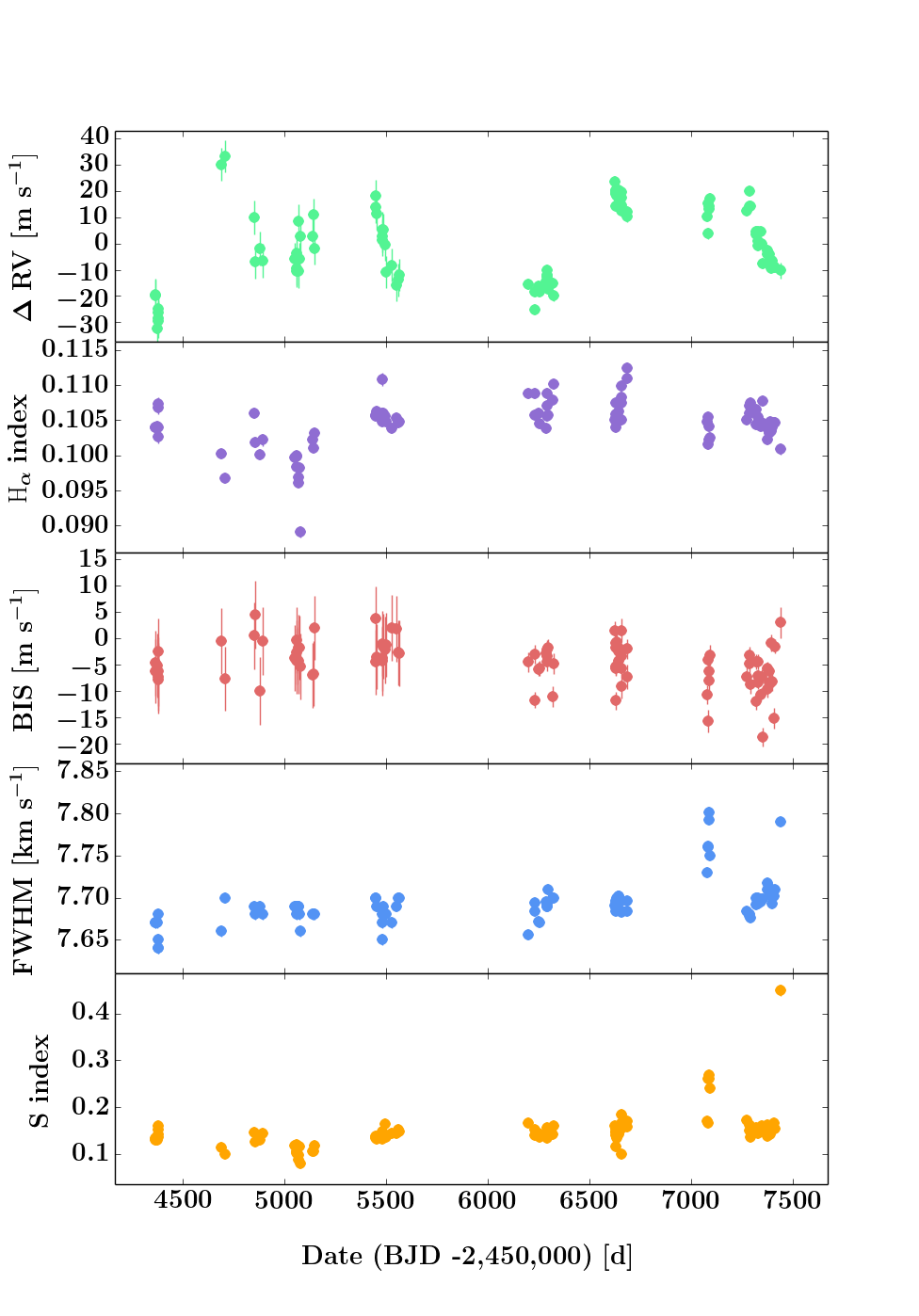
Figure 1: SOPHIE activity indicators for HD17674.

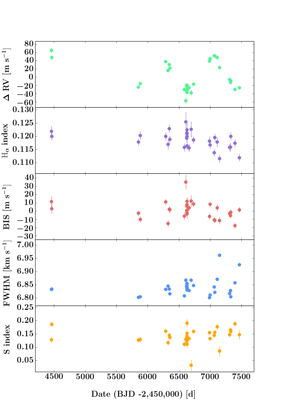
Figure 2: SOPHIE activity indicators for HD42012.

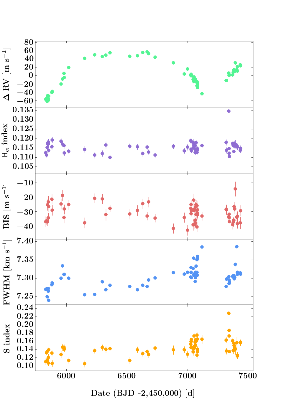
Figure 3: SOPHIE activity indicators for HD29021.

4 Data analysis

4.1 Method

ELODIE and SOPHIE radial velocities were fitted using the tools available in the Data and Analysis Center for Exoplanets (DACE) developed by the National Centre of Competence in Research PlanetS. A preliminary solution is found using a periodogram of RVs which, for all three targets, shows clear peaks at the periods of each orbit. The analytical method used for computing the orbital parameters from the periodogram of RVs is described in detail in Delisle et al. (2016). The results of this first analytical approximation are used as uniform priors for a Markov chain Monte Carlo (MCMC) model that we used to determine our final parameters and errors. The algorithm used for the MCMC is described in detail in Díaz et al. (2014, 2016b). For the MCMC, we fit five parameters of the Keplerian orbit and a linear drift (to set the intervals in Table 3). For HD17674, we also fit the instrumental offset between SOPHIE and ELODIE. For HD42012 the offset is fixed using Boisse et al. (2012) since we only use the ELODIE point to constrain any possible long-term drift. We did not model the stellar jitter because these targets are non-active G and K dwarfs and because no correlations with the activity indicators were found. For the orbital parameters, listed in Table 3, we used the mode estimate and the errors corresponding to the 68.3% confidence intervals. For the detection limits mentioned in sections 5.1 through 5.3, in the residuals we injected planets in circular orbits at different trial periods. Using a generalized Lomb-Scargle periodogram, an injected planet is considered detected when the false alarm probability is lower than $1\%$.

4.2 Astrometric analysis

We analysed the astrometric data available from the Hipparcos mission (ESA 1997) to search for signatures of orbital motion. We employed the new Hipparcos reduction (van Leeuwen 2007) and followed the procedure described in Sahlmann et al. (2011b). No significant orbital signals were detected in the Hipparcos astrometry for these stars. As was done in previous works (e.g. Díaz et al. 2012) by using the Hipparcos data and the parameters found from the RV analysis, we were able to set upper mass limits for two of the companions. For HD17674, the upper mass limit of the companion is 89 $M_{Jup}$, and for HD42012 it is 67 $M_{Jup}$. No constraints could be established for HD29021 since the orbital period is not covered by Hipparcos data.

5 Results

5.1 HD17674

HD17674 was observed with both ELODIE and SOPHIE spectrographs with, respectively, 8 and 93 measurements for a total time span of over 18 years. One ELODIE point was excluded from the analysis, due to low S/N. For the same reason, nine SOPHIE points were not considered. Due to abnormal flux levels of the thorium-argon lamp, eight measurements were excluded. The 18 points that were excluded do not significantly change the solution we find, and would only increase the value of $\sigma_{(O-C)}$.
HD17674 is a V = 7.56 mag G0V star with a mass of $M_{*}$ of $0.98\pm 0.10M_{\odot}$ located at 44.5 parsecs from the Sun. The parameters of the Keplerian fit are listed in Table 3 and the orbital solution is shown in Fig. 4.
Our analysis indicates the presence of a companion of minimum mass M${}_{c}\sin i=0.9$ M_Jup on a 1.7-year orbit (see Fig. 4). We find a non-significant eccentricity with an upper $3\sigma$ limit of $e=0.13$. No significant long-term drift was detected in the data, and we can exclude giant planets more massive than M${}_{c}\sin i=2.4$ M_Jup on circular orbits shorter than 37 years. In Table 3 we included the 99% confidence intervals for this value. This target was also observed in high cadence to discard the presence of an inner companion. The periodogram of the residuals can be seen in Fig. 4 and does not show any significant signals. We can exclude the presence of giant planets more massive than 0.05 and 0.1 M_Jup with periods shorter than 10 and 100 days, respectively. The dispersion of the residuals (Table 3) corresponds well to the expected precision for each instrument.
The instrumental offset between ELODIE and SOPHIE was left as a free parameter and was adjusted to $57\pm 6$ $ms^{-1}$, in agreement with the expected offset at $46\pm 23$ $ms^{-1}$ (Boisse et al. 2012).
In addition, we followed the procedure described by Díaz et al. (2016a) to calculate the luminosity of HD17674 and to check whether the planet was in the habitable zone. We used the habitable zone calculator based on the work by Kopparapu et al. (2013). We chose the Runaway Greenhouse limit for our inner limit and the Maximum Greenhouse limit as the outer one. This yields a habitable zone between 1.2 AU and 2.1 AU. With a semi-major axis of 1.42 AU and an almost circular orbit, HD17674 b falls well inside this region. This is important for habitability if exomoons can be detected with future techniques around this kind of target. Since HD17674 is an evolved star, it is possible that the detected planet was outside the habitable zone when the star was still in the main sequence.

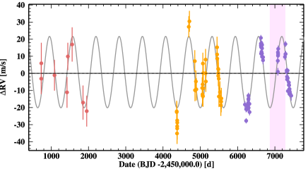
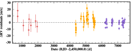
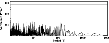
Figure 4: Radial velocity curve (top) and residuals (middle) of HD17674. ELODIE data shown in red, SOPHIE in orange, and SOPHIE+ in purple. The region in pink indicates the Gaia observation dates for DR1. Generalized Lomb-Scargle (GLS) periodogram (bottom) of the radial velocities after subtraction of the planetary orbit. False alarm probability lines are plotted for 50%, 10%, and 1%.

5.2 HD42012

HD42012 was observed once with ELODIE in thosimult mode in March 2004, twice with SOPHIE before the upgrade, and 29 times with SOPHIE+ for a total duration of 12 years. No measurements were excluded from the analysis. The star is a V = 8.44 mag K0 star with a mass of $M_{*}$ of $0.83\pm 0.08M_{\odot}$ located at 37.1 parsecs from the Sun.
The Keplerian fit (see Fig. 5) indicates the presence of a companion of minimum mass M${}_{c}\sin i=1.6$ M_Jup on a 2.3-year orbit. We find a non-significant eccentricity with an upper $3\sigma$ limit of $e=0.20$. All parameters are listed in Table 3.
The offset between ELODIE and SOPHIE was fixed using Boisse et al. (2012), which yields an absolute value of $134\pm 23$ $ms^{-1}$. We decided not to fit this parameter as we did for HD17674; in this case, only one ELODIE point was available and thus the offset fitting would not be informative. Thanks to this additional point we can rule out any significant long-term drift. We can exclude giant planets more massive than M${}_{c}\sin i=2.1$ M_Jup on circular orbits shorter than 16 years. In Table 3 we included the 99% confidence intervals for this value. The periodogram of the residuals can be seen in Fig. 5 and it shows that no other significant signals are present in the data. The dispersion of the residuals is higher than expected for the precision of the instruments, which can indicate for example that we underestimated the activity level or there is an additional undetected companion. Nevertheless, we can exclude the presence of giant planets more massive than 0.06 and 0.02 M_Jup with periods shorter than 10 and 100 days, respectively.
Following the same habitable zone analysis, this planet lies beyond the Maximum Greenhouse limit of HD42012.

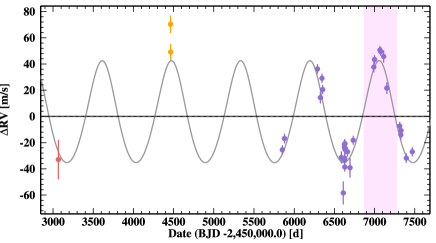
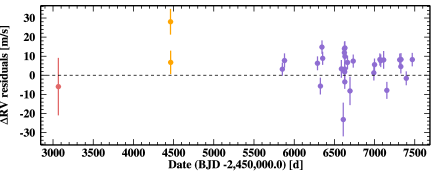
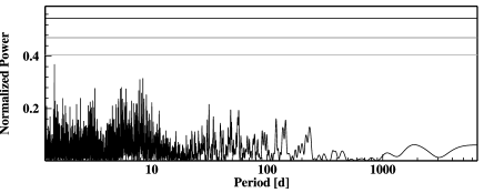
Figure 5: Radial velocity curve (top) and residuals (middle) of HD42012. GLS periodogram (bottom) of the RVs after subtraction of the planetary orbit. Colours and symbols are the same as in Fig.4.

Table 3: Orbital parameters

Parameters	HD17674	HD42012	HD29021
P [days](1)	$623.8^{+1.6}_{-1.5}$	$857.5^{+6.2}_{-6.3}$	$1362.3^{+4.6}_{-4.0}$
K [ms-1](1)	$21.1^{+0.6}_{-0.5}$	$39.0\pm 0.9$	$56.4\pm 0.9$
e (1)	$<0.13$	$<0.2$	$0.459\pm 0.008$
$T_{p}$ [RJD](1)	$2455904.8\pm 3$	$2455386.2\pm 10$	$2455823.9^{+6.1}_{-5.7}$
$\omega$ [deg](1)	-	-	$179.5\pm 2.0$
$a$ [AU](1)	$1.42^{+0.04}_{-0.05}$	$1.67^{+0.05}_{-0.06}$	$2.28^{+0.07}_{-0.08}$
M${}_{c}\sin i$ [MJup](1)	$0.87^{+0.07}_{-0.06}$	$1.6\pm 0.1$	$2.4\pm 0.2$
ELODIE $\sigma$(res) [ms-1]	8.24	7.73	-
SOPHIE $\sigma$(res) [ms-1]	8.23	20.07	-
SOPHIE+ $\sigma$(res) [ms-1]	3.12	8.61	3.93
RV drift [m s-1 yr-1](2)	[-0.7;+2.2]	[-3.9;-0.1]	[-3.2;+0.6]

⁽¹⁾Uncertainties correspond to the 68.3% confidence intervals.
⁽²⁾ 99% confidence intervals.

5.3 HD29021

HD29021 was only observed with SOPHIE+ with 66 measurements spanning almost 4.5 years. Two measurements were excluded from the analysis owing to low S/N. Nevertheless, their presence did not affect the resulting orbit in a significant way. The star is a V = 7.76 mag G5 star with a mass of $M_{*}$ of $0.85\pm 0.08M_{\odot}$ located at 30.6 parsecs from the Sun.
The solution we find (see Fig. 6) corresponds to a companion of minimum mass M${}_{c}\sin i=2.4$ M_Jup on a 3.7-year eccentric orbit. All orbital parameters are listed in Table 3. No significant long-term drift was detected in the data, and we can exclude giant planets more massive than M${}_{c}\sin i=1.2$ M_Jup on circular orbits shorter than 9 years. In Table 3 we included the 99% confidence intervals for this value. The periodogram of the residuals is shown in Fig. 6 and, as in the previous cases, no other significant signals are present in the data. The dispersion of the residuals is also within the expected levels for SOPHIE+. We can exclude the presence of giant planets more massive than 0.1 and 0.3 M_Jup with periods shorter than 10 and 100 days, respectively.
Following the same analysis as before, this planet lies beyond the outer limit of the habitable zone of HD29021.

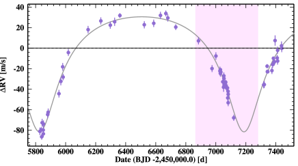
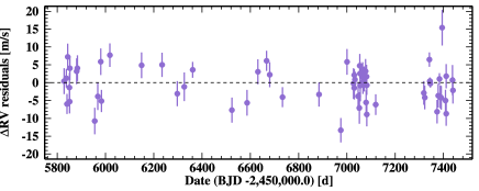
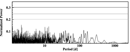
Figure 6: Radial velocity curve (top) and residuals (middle) of HD29021. GLS periodogram (bottom) of the RVs after subtraction of the planetary orbit. Colours and symbols are the same as in Fig.4.

6 Gaia astrometry

Due to the characteristics of our planets and their host stars, we were also interested in studying the expected astrometric detection with Gaia and its microarcsecond precision. In this section, we will discuss four different approaches.
In astrometry, several factors will determine the detectability of a planet, the number of field crossings of the star and their distribution, the orbital period of the planet, the orbital phase of elliptical orbits, and of course the mission duration. The periods for which Gaia will be most efficient are $0.2\lesssim P\lesssim 6$ years (Perryman et al. 2014), so our periods between 1.7 and 3.7 years are well in this interval, which means that at least one full orbit will be covered during the five-year mission of Gaia. Casertano et al. (2008) estimated from their numerical double-blind simulations that a planet will be detected by Gaia with a small number of false positives, if the astrometric signal-to-noise per field crossing $S/N_{1meas}>3$ and the period $P\leq 5$ years. The value $S/N_{1meas}$ will be the first estimator that we will discuss. It is defined as $S/N_{1meas}\equiv\alpha/\sigma_{fov}$, where $\sigma_{fov}$ is the accuracy of a single field-of-view crossing and $\alpha$ is the astrometric signature given by

$$\alpha=\left(\frac{M_{p}}{M_{Jup}}\right)\left(\frac{M_{\star}}{M_{\odot}}\right)^{-1}\left(\frac{a_{p}}{1AU}\right)\left(\frac{d}{1pc}\right)^{-1}*954.6\quad\mu as,$$ (1)

for a circular orbit. Values for our three planets are listed in Table 4. As in Perryman et al. (2014), we take the latest estimates of $\sigma_{fov}=34.2$ $\mu as$, which is constant for targets with magnitude G$\leq$12 in the G band of Gaia. Using the detection criterion of Casertano et al. (2008) and $\sigma_{fov}=34.2$ $\mu as$, a planet around a star with magnitude G$\leq$12 and period $P\leq 5$ years would be detectable by Gaia if $\alpha\gtrsim 103$ $\mu as$. According to this, HD29021 b could be detected by Gaia alone. Since this target is eccentric, in Table 4 we gave an estimate of the maximum value of $\alpha$ when the planet is at apastron. In Fig. 6 we can also see which part of the orbit was covered by Gaia DR1. For their final number of detections, Perryman et al. (2014) consider that a more liberal threshold of $S/N_{1meas}>2$ is a reasonable approximation. In this case, we would need $\alpha\gtrsim 68$ $\mu as$ and hence HD42012 b could also be detected.

As Perryman et al. (2014) indicate in their work, while $S/N_{1meas}$ provides some indication of planet detection numbers, it is a simplistic approach. So as a second estimate, we calculate the expected signal-to-noise at the end of the mission $S/N_{Nmeas}$ (see Table 4) using the number of measurements provided by the Gaia Observation Forecast Tool. If we combine astrometric data with RVs, an astrometric orbit could be retrieved with an astrometric signal-to-noise down to 6.2 (Sahlmann et al. 2011a). By the end of the mission, all three planets could be detected using a combined analysis with estimated values of $S/N_{Nmeas}=8.0$, $19.5$, and $69.2$ for HD17674, HD42012, and HD29021, respectively.

Table 4: Data from Gaia DR1 and estimated values. The number of Gaia observations is determined for each target using the Gaia Observation Forecast Tool. The S/N is calculated for one measurement, the measurements available in DR1, and the expected values at the end of the mission.

Target	$\alpha$	Nmeas	Nmeas	S/N1meas	S/NNmeas	Astrometric Excess Noise	$\Delta Q$
Name	[$\mu as$]	DR1	End of Mission			[mas]
HD17674	27	32(1)	101	0.8	8.0	0.33	3.04
HD42012	83	5(1)	66	2.4	19.5	0.28	-
HD29021	201(2)	14(1)	133	6.0	69.2	0.52	2.15

⁽¹⁾ Number of matched observations from the Gaia archive. Using the Forecast Tool, the expected number of observations were 35, 5 and 19 respectively.
⁽²⁾ The detectability of eccentric orbits will vary over the orbital phase, so the astrometric signal given for HD29021 corresponds to apastron.

The Gaia DR1 released in September 2016 (Lindegren et al. 2016) contains provisional astrometric results for over one billion sources brighter than G magnitude 20.7 for the first 418 days of the mission. Using DR1, we discuss a third indicator. An orbiting companion of planetary mass will produce a perturbation in the stellar motion, and this will be reflected as a deviation of the astrometric data from the five-parameter model. In Gaia DR1, this value is called astrometric excess noise $\epsilon_{i}$ [mas] and is listed in Table 4. As Lindegren et al. (2016) describe in their work, $\epsilon_{i}=0$ when the source is astrometrically well behaved, and a value larger than 0 indicates that the residuals are statistically larger than expected. But since DR1 only presents a preliminary solution, the calibration modelling errors are high and this leads to a significant value ($\sim$ 0.5 mas) of the astrometric excess noise for nearly all sources. Nevertheless, Lindegren et al. (2016) also mention that a source with a value of $\epsilon_{i}$ above 1-2 mas could indicate the presence of an astrometric binary or a problematic source. This is not the case for any of the $\epsilon_{i}$ listed in Table 4. This is especially important for HD29021 b where we could not set an upper-mass limit from the Hipparcos data.

A final indicator worth mentioning is the astrometric $\Delta Q$. This quantity is defined for the Tycho-Gaia (TGAS) astrometric solution and it is sensitive to the difference of Hipparcos and TGAS proper motions. It was first introduced by Michalik et al. (2014), in the context of the Hundred Thousand Proper Motions project, and was also used by Lindegren et al. (2016) in their work on Gaia DR1 with a slightly different definition of the parameter that only considers the differences on proper motions
For single stars, $\Delta Q$ is expected to follow a chi-squared distribution with two degrees of freedom (Lindegren et al. 2016). Deviations from this theoretical distribution could be caused, for example, by binaries with periods of 10-50 years that will have increased values of $\Delta Q$ (Michalik et al. 2014). This latter work also demonstrated a strong dependency of $\Delta Q$ on the quality of the Gaia solution, so even though the full sensitivity of this parameter is not reached in DR1, it will increase in the next Gaia releases. We compared the $\Delta Q$ values of the present TGAS solution for our targets (see Table 4) with Fig. C.3 of Lindegren et al. (2016). Our values are not significantly high and are placed in the region where the highest relative frequency is expected, near the theoretically expected distribution.

7 Discussion and conclusions

We have reported the detection of three new Jupiter-mass companions orbiting the solar-type stars HD17674, HD29021, and HD42012. We found no evidence of additional giant companions. As a reference for this population of objects, as of October 2016, the exoplanets.eu database (Schneider et al. 2011) listed around 200 planets with masses between 0.8 and 15 M_Jup and periods longer than 600 days.
The three host stars present a subsolar metallicity, which is unusual for stars with giant planetary companions (Johnson et al. 2010), but also reinforces the result found by Adibekyan et al. (2013), who showed that planets orbiting metal-poor stars have longer periods than those around metal-rich ones. The fact that these companions all make, as far as our analysis can tell, single giant-planet systems, may also be linked to the low heavy-element content of their birth nebulosity.
We expect that for the last Gaia data release (programmed for 2022) these three new planets will be fully characterized with a joint astrometric and radial velocity analysis.

1]

Table 5: Radial velocities of HD17674.

BJD	RV	$\sigma(RV)$	Instrument
$[-2400000$ $days]$	[$km/s$]	[$km/s$]
50731.5728	10.547	0.009	ELODIE
50733.5803	10.556	0.012	ELODIE
51087.6079	10.549	0.009	ELODIE
51423.6193	10.539	0.009	ELODIE
51445.6047	10.560	0.008	ELODIE
51560.3474	10.567	0.010	ELODIE
51853.5015	10.533	0.010	ELODIE
51952.3135	10.528	0.009	ELODIE
54366.6249	10.5851	0.0062	SOPHIE
54367.6473	10.5847	0.0061	SOPHIE
54375.5863	10.5722	0.0061	SOPHIE
54379.5426	10.5764	0.0064	SOPHIE
54379.5452	10.5798	0.0064	SOPHIE
54379.5478	10.5751	0.0065	SOPHIE
54381.4875	10.5785	0.0062	SOPHIE
54689.6326	10.6346	0.0062	SOPHIE
54707.6312	10.6378	0.0061	SOPHIE
54852.3384	10.6145	0.0064	SOPHIE
54857.3196	10.5975	0.0064	SOPHIE
54881.2713	10.6026	0.0064	SOPHIE
54894.3095	10.5980	0.0065	SOPHIE
55050.6272	10.5988	0.0062	SOPHIE
55059.6243	10.5951	0.0062	SOPHIE
55061.6267	10.5942	0.0061	SOPHIE
55062.6359	10.6009	0.0062	SOPHIE
55068.6137	10.6131	0.0063	SOPHIE
55071.6209	10.5940	0.0062	SOPHIE
55075.6095	10.5986	0.0061	SOPHIE
55078.6028	10.6075	0.0063	SOPHIE
55140.5422	10.6074	0.0062	SOPHIE
55141.5476	10.6154	0.0062	SOPHIE
55148.4721	10.6026	0.0061	SOPHIE
55449.6038	10.6226	0.0062	SOPHIE
55450.5773	10.6184	0.0061	SOPHIE
55453.6185	10.6160	0.0062	SOPHIE
55479.5179	10.6100	0.0065	SOPHIE
55481.5293	10.6059	0.0061	SOPHIE
55483.5386	10.6075	0.0062	SOPHIE
55484.4508	10.6097	0.0062	SOPHIE
55495.4945	10.6042	0.0063	SOPHIE
55498.4640	10.5938	0.0061	SOPHIE
55527.4474	10.5964	0.0063	SOPHIE
55551.4847	10.5887	0.0062	SOPHIE
55559.2883	10.5908	0.0062	SOPHIE
55564.3481	10.5927	0.0062	SOPHIE
56197.6216	10.5891	0.0019	SOPHIE+
56229.5802	10.5864	0.0018	SOPHIE+
56230.6107	10.5796	0.0015	SOPHIE+
56251.5219	10.5885	0.0014	SOPHIE+
56252.4853	10.5864	0.0014	SOPHIE+
56285.3763	10.5901	0.0014	SOPHIE+
56290.4409	10.5920	0.0017	SOPHIE+
56291.4018	10.5943	0.0017	SOPHIE+
56292.4112	10.5925	0.0019	SOPHIE+
56296.4632	10.5872	0.0016	SOPHIE+
56318.2903	10.5895	0.0020	SOPHIE+
56321.3202	10.5847	0.0019	SOPHIE+
56625.4795	10.6281	0.0017	SOPHIE+
56626.3869	10.6248	0.0017	SOPHIE+
56627.3911	10.6235	0.0016	SOPHIE+
56628.3784	10.6238	0.0016	SOPHIE+
56629.3792	10.6189	0.0015	SOPHIE+
56630.3612	10.6244	0.0014	SOPHIE+
56631.3437	10.6227	0.0014	SOPHIE+
56641.3450	10.6249	0.0016	SOPHIE+
56642.4651	10.6200	0.0016	SOPHIE+
56643.4579	10.6225	0.0014	SOPHIE+
56654.3328	10.6190	0.0017	SOPHIE+
56655.4128	10.6171	0.0024	SOPHIE+
56656.3454	10.6220	0.0020	SOPHIE+
56657.3921	10.6240	0.0022	SOPHIE+
56682.3844	10.6150	0.0023	SOPHIE+
56683.2899	10.6168	0.0019	SOPHIE+
57079.2841	10.6147	0.0018	SOPHIE+
57081.3406	10.6083	0.0022	SOPHIE+
57082.2718	10.6197	0.0014	SOPHIE+
57084.3132	10.6177	0.0016	SOPHIE+
57088.3042	10.6187	0.0018	SOPHIE+
57090.2717	10.6217	0.0019	SOPHIE+
57270.5852	10.6170	0.0019	SOPHIE+
57283.5606	10.6186	0.0017	SOPHIE+
57284.5766	10.6245	0.0017	SOPHIE+
57289.6718	10.6187	0.0018	SOPHIE+
57318.5297	10.6091	0.0015	SOPHIE+
57319.5255	10.6081	0.0014	SOPHIE+
57326.5356	10.6054	0.0013	SOPHIE+
57327.5446	10.6091	0.0014	SOPHIE+
57328.4815	10.6038	0.0014	SOPHIE+
57342.5121	10.6090	0.0013	SOPHIE+
57345.4750	10.6046	0.0015	SOPHIE+
57349.4221	10.5970	0.0018	SOPHIE+
57373.4358	10.6005	0.0013	SOPHIE+
57375.4532	10.6020	0.0016	SOPHIE+
57383.3395	10.5978	0.0014	SOPHIE+
57384.3697	10.6004	0.0014	SOPHIE+
57385.4349	10.5973	0.0016	SOPHIE+
57393.4056	10.5952	0.0016	SOPHIE+
57394.3422	10.5982	0.0018	SOPHIE+
57404.3579	10.5958	0.0020	SOPHIE+
57412.2578	10.5954	0.0013	SOPHIE+
57440.3545	10.5943	0.0029	SOPHIE+

Table 5: Continued.

1]

Table 6: Radial velocities of HD42012.

BJD	RV	$\sigma(RV)$	Instrument
$[-2400000$ $days]$	[$km/s$]	[$km/s$]
53066.3767	41.3738	0.0150	ELODIE
54461.5393	41.4771	0.0067	SOPHIE
54463.5387	41.4559	0.0061	SOPHIE
55852.5515	41.3813	0.0034	SOPHIE+
55879.5723	41.3899	0.0037	SOPHIE+
56289.5602	41.4430	0.0036	SOPHIE+
56326.3670	41.4211	0.0044	SOPHIE+
56345.3569	41.4359	0.0035	SOPHIE+
56354.3659	41.4273	0.0034	SOPHIE+
56587.6472	41.3755	0.0046	SOPHIE+
56610.6909	41.3484	0.0088	SOPHIE+
56624.5463	41.3834	0.0035	SOPHIE+
56625.5848	41.3855	0.0036	SOPHIE+
56627.6562	41.3734	0.0053	SOPHIE+
56628.6200	41.3749	0.0059	SOPHIE+
56629.4549	41.3682	0.0036	SOPHIE+
56630.4946	41.3860	0.0035	SOPHIE+
56631.5222	41.3816	0.0035	SOPHIE+
56663.4586	41.3798	0.0035	SOPHIE+
56694.3507	41.3676	0.0074	SOPHIE+
56734.4235	41.3886	0.0034	SOPHIE+
56990.5750	41.4444	0.0040	SOPHIE+
56999.5758	41.4502	0.0032	SOPHIE+
57066.4235	41.4574	0.0032	SOPHIE+
57076.3480	41.4563	0.0033	SOPHIE+
57113.3182	41.4525	0.0046	SOPHIE+
57152.3236	41.4284	0.0044	SOPHIE+
57312.6930	41.3994	0.0033	SOPHIE+
57326.7115	41.3927	0.0036	SOPHIE+
57328.6237	41.3960	0.0033	SOPHIE+
57394.5206	41.3750	0.0036	SOPHIE+
57469.3745	41.3798	0.0035	SOPHIE+

Table 6: Continued.

1]

Table 7: Radial velocities of HD29021.

BJD	RV	$\sigma(RV)$	Instrument
$[-2400000$ $days]$	[$km/s$]	[$km/s$]
55828.6566	0.4326	0.0036	SOPHIE+
55837.6068	0.4341	0.0026	SOPHIE+
55840.6330	0.4273	0.0028	SOPHIE+
55843.6102	0.4410	0.0037	SOPHIE+
55850.5553	0.4339	0.0041	SOPHIE+
55851.5737	0.4302	0.0033	SOPHIE+
55852.5084	0.4398	0.0034	SOPHIE+
55880.4888	0.4490	0.0036	SOPHIE+
55883.5563	0.4512	0.0036	SOPHIE+
55955.4716	0.4693	0.0037	SOPHIE+
55968.3043	0.4813	0.0038	SOPHIE+
55980.3807	0.4955	0.0037	SOPHIE+
55983.2592	0.4855	0.0031	SOPHIE+
56018.2942	0.5094	0.0033	SOPHIE+
56149.6362	0.5317	0.0036	SOPHIE+
56234.5222	0.5402	0.0034	SOPHIE+
56297.4726	0.5361	0.0035	SOPHIE+
56326.2884	0.5394	0.0040	SOPHIE+
56361.3075	0.5455	0.0022	SOPHIE+
56523.6341	0.5365	0.0035	SOPHIE+
56586.6136	0.5379	0.0036	SOPHIE+
56631.4207	0.5456	0.0035	SOPHIE+
56667.3642	0.5475	0.0028	SOPHIE+
56680.3360	0.5431	0.0035	SOPHIE+
56733.3712	0.5342	0.0028	SOPHIE+
56884.6237	0.5208	0.0034	SOPHIE+
56974.6637	0.4938	0.0034	SOPHIE+
57000.5342	0.5060	0.0036	SOPHIE+
57027.3511	0.4914	0.0043	SOPHIE+
57030.4164	0.4891	0.0032	SOPHIE+
57030.4229	0.4927	0.0017	SOPHIE+
57033.3788	0.4904	0.0022	SOPHIE+
57046.3508	0.4809	0.0040	SOPHIE+
57051.4553	0.4756	0.0044	SOPHIE+
57053.3122	0.4867	0.0033	SOPHIE+
57054.3412	0.4841	0.0032	SOPHIE+
57055.3789	0.4803	0.0044	SOPHIE+
57063.2819	0.4795	0.0022	SOPHIE+
57064.3056	0.4803	0.0019	SOPHIE+
57065.3232	0.4806	0.0021	SOPHIE+
57066.3215	0.4767	0.0033	SOPHIE+
57071.3543	0.4756	0.0033	SOPHIE+
57072.3032	0.4748	0.0033	SOPHIE+
57077.3605	0.4749	0.0034	SOPHIE+
57079.4398	0.4652	0.0034	SOPHIE+
57081.3098	0.4716	0.0033	SOPHIE+
57082.3654	0.4605	0.0033	SOPHIE+
57082.3682	0.4687	0.0027	SOPHIE+
57119.3022	0.4458	0.0029	SOPHIE+
57318.5711	0.4779	0.0033	SOPHIE+
57322.5186	0.4782	0.0033	SOPHIE+
57341.6912	0.4961	0.0020	SOPHIE+
57343.5214	0.4907	0.0010	SOPHIE+
57344.5119	0.4910	0.0010	SOPHIE+
57345.5194	0.4907	0.0011	SOPHIE+
57373.5202	0.4918	0.0033	SOPHIE+
57378.3850	0.4977	0.0033	SOPHIE+
57383.4111	0.5038	0.0016	SOPHIE+
57386.4651	0.4996	0.0032	SOPHIE+
57390.4414	0.5004	0.0033	SOPHIE+
57394.4581	0.5211	0.0050	SOPHIE+
57408.5114	0.5041	0.0030	SOPHIE+
57411.3967	0.5116	0.0034	SOPHIE+
57411.4415	0.5011	0.0034	SOPHIE+
57437.3516	0.5160	0.0042	SOPHIE+
57439.2881	0.5135	0.0037	SOPHIE+

Table 7: Continued.