Automatic implementation of material laws: Jacobian calculation in a finite element code with TAPENADE

Abstract

In an effort to increase the versatility of finite element codes, we explore the possibility of automatically creating the Jacobian matrix necessary for the gradient-based solution of nonlinear systems of equations. Particularly, we aim to assess the feasibility of employing the automatic differentiation tool TAPENADE for this purpose on a large Fortran codebase that is the result of many years of continuous development. As a starting point we will describe the special structure of finite element codes and the implications that this code design carries for an efficient calculation of the Jacobian matrix. We will also propose a first approach towards improving the efficiency of such a method. Finally, we will present a functioning method for the automatic implementation of the Jacobian calculation in a finite element software, but will also point out important shortcomings that will have to be addressed in the future.

AICES

1 Introduction

In the field of numerical simulations, a central task that needs to be accomplished is the solution of partial differential equations (PDEs). When such equations are discretized, the result is a system of equations. For a set of nonlinear partial differential equations, the discretized equations are also nonlinear.

A very popular method for the solution of nonlinear systems of equations is the Newton–Raphson iteration scheme [1]. If a nonlinear system of equations for a vector of unknowns $\mathbf{u}$ is given by

$$\mathbf{F}(\mathbf{u})\;=\;\mathbf{0}\,,$$ (1)

then, starting from an initial guess $\mathbf{u}_{0}$, one iteration step of the Newton–Raphson scheme is given by

$$\frac{\partial\mathbf{F}(\mathbf{u}^{k})}{\partial\mathbf{u}}\cdot\Delta\mathbf{u}^{k+1}\;=\;-\mathbf{F}(\mathbf{u}^{k})\,,$$ (2)

which defines a linear system of equations.

There are many different methods for the solution of the resulting linear equation systems. Some of these require the full Jacobian matrix $\frac{\partial\mathbf{F}(\mathbf{u}^{k})}{\partial\mathbf{u}}$. Others, especially Krylov-based methods such as GMRES [2, §3], require matrix-vector products, which would be directional derivatives of $\mathbf{F}(\mathbf{u})$ in this context. These methods can be implemented in such a way that the Jacobian matrix does not need to be calculated explicitly. They are called matrix-free methods [3, §3], [4]. However, the combination of such a method with a general-purpose preconditioner usually requires the full matrix again. For this reason, we will only consider the accumulation of the full Jacobian matrix.

It is very common to implement the calculation of this matrix directly into the program code. In these cases, the residual $\mathbf{F}(\mathbf{u})$ first needs to be differentiated with respect to the vector of unknowns $\mathbf{u}$, which could, for instance, be done manually. The process of differentiating the residual and subsequently implementing the derivative depends entirely on the differential equations in use and needs to be repeated whenever these equations are changed. Using this method, the task of trying out new simulation models may require considerable effort. Additionally, a manual derivation and implementation of the derivative invites mistakes that may be very hard to find later on. As an alternative, there is also the option of obtaining the derivative by an automated procedure.

There exist different approaches of this kind, and they typically require a program function that calculates the residual $\mathbf{F}(\mathbf{u})$ to work with. The oldest and simplest method would be a finite-difference (FD) approximation. This just requires repeated calls to the residual function with a perturbed input $\mathbf{u}+\Delta\mathbf{u}$ to obtain a directional derivative. This method has been used for the estimation of Jacobian matrices for a long time, and some techniques for increased efficiency have also been developed. For example, if the sparsity pattern of the Jacobian is known beforehand, an optimized seed matrix can be used to calculate a compressed Jacobian [5].

In the last decades, there has been a lot of interest in using the method of automatic differentiation (AD) [6, 7] for this purpose. Recent examples of such approaches are described in [8] and [9]. The methods for sparsity exploitation that were developed for finite-difference approaches can easily be transferred to the similar forward mode of automatic differentiation, but more complex possibilities have also been researched [10, 11, 12, 13].

The most important advantage of AD over FD is that the resulting derivatives obtained this way are generally more accurate, since they do not suffer from possible cancellation errors that limit the number of significant digits. Unfortunately, this improved accuracy comes at the cost of a much more difficult and laborious implementation. Our aim in this paper is to investigate the suitability and efficiency of using AD for the Jacobian calculation specifically in the context of finite element (FE) codes.

We decided to use the forward mode of automatic differentiation, since we expect this to be more efficient for the calculation of a square Jacobian matrix (see Section 2.1). Our research focuses on the implementation of the Jacobian calculation in a specific finite element code written in Fortran. Of the different techniques that are available for the implementation of automatic differentiation, we consider source code transformation to be more suitable for Fortran codes (see Section 2.1).

There are a number of programs available that support automatic differentiation by code source transformation in Fortran codes. One of the earliest was ADIFOR [14, 15], which seems to have been under development mostly in the 1990s. Another early implementation was Odyssée [16], which was later replaced by TAPENADE [17]. Other software includes OpenAD/F [18]. The present work will focus on the investigation of TAPENADE as a tool for the automatic differentiation. This decision is motivated primarily by the long history of this software and its widespread use in the scientific community.

One should note that even though we made some specific choices, many of the findings we present in this document can be applied universally, i.e., they apply for arbitrary modes or techniques of automatic differentiation or even for arbitrary software.

Our principal aim of calculating a Jacobian matrix via forward mode AD can easily be achieved using repetitive calculations of directional derivatives. This is analogous to the approach used with finite-difference methods. In cases where the Jacobian matrix is sparse, more efficient techniques can be applied, provided that the sparsity pattern is known beforehand (see, e.g., [5], where this is discussed in relation to the finite differences method). We will show that the Jacobian matrix resulting from the finite element discretization is indeed sparse (see Section 3.1). Since its sparsity pattern depends on the computational mesh, conventional methods of sparsity exploitation are not suitable. We will describe an alternative way of calculating the matrix efficiently, that utilizes structures that are commonly found in finite element codes.

We will provide some background on relevant aspects of automatic differentiation in Section 2.1. Section 2.2 gives an overview of the software programs in use as well as the difficulties arising from their combination. We will describe the development of a suitable procedure for the automatic creation of the Jacobian matrix in a finite element code in Section 3.2, and present the results that we obtained when using it on a viscoelastic flow problem in Section 4.

2 Automatic differentiation with TAPENADE

2.1 Automatic differentiation

The term automatic differentiation describes the differentiation of program functions, when it is carried out by computer algorithms. It is based on the idea that certain program functions can be viewed as sequences of mathematical expressions [6]. Assuming existence, derivatives of these individual expressions can be calculated and used in the chain rule to determine the full function derivative [7].

Concerning the order in which the individual derivatives are calculated, one generally distinguishes between a forward and a reverse mode [7, 19]. In forward mode, the calculation of the derivatives happens in the same order as the execution of the original statements. This means that at an arbitrary point during the calculation, the derivatives of all relevant intermediate variables with respect to the input variable are known. In reverse mode, on the other hand, the operations are carried out in reverse order. Therefore, the quantities that are available during the calculation are the derivatives of the output variable with respect to the relevant intermediate variables. In analogy to the matrix multiplication, where the transposition also inverts the order in which the matrices are multiplied, these quantities are often called adjoints [10, 7, 14]. In summary, the result of forward mode AD will be a matrix-vector product, $\frac{\partial\mathbf{F}}{\partial\mathbf{u}}\cdot\mathbf{e}$, for some vector $\mathbf{e}$, and the result of reverse mode AD will be a vector-matrix product, $\mathbf{e}^{T}\cdot\frac{\partial\mathbf{F}}{\partial\mathbf{u}}$.

In order to be able to carry out the derivative calculations in reverse order, reverse mode requires all operations to be recorded, e.g., in a graph representing the program structure. This imposes greater requirements on system memory [19].

For the calculation of quadratic Jacobian matrices, the same number of runs of the derivative function are required, independently of the selected mode. However, the forward mode promises both an easier implementation and lower memory requirements under these conditions.

In addition to the different modes for ordering the derivative evaluations, there are also different methods how to implement them. The most popular methods are source code transformation and operator overloading.

Source code transformation methods aim to work with arbitrary function code that should ideally not require any preparations. In order to calculate the derivatives, an additional code transformation step is added between preprocessing and compiling of the source code [15].

In contrast, operator overloading methods require the use of special data types in the function code. Overloaded versions of all mathematical operations exist for these data types, such that it is possible to either evaluate a derivative or accumulate some representation of a computational graph during function execution [20].

In some contexts, source code transformation methods have been shown to be superior to operator overloading methods, in terms of runtime efficiency [21, 22]. It also makes a huge difference which programming language is used. The operator overloading method of AD requires object-oriented programming, which can be done quite efficiently in a language such as C++. In Fortran, on the other hand, such concepts have only recently been added to the language, and are therefore less flexible and their usage may incur performance losses. The switch from a function code using intrinsic data types to an object type suitable for AD with operator overloading would also require great changes in a Fortran code, which may not be easy to automatize.

For further details on the different modes and implementation methods, we refer to [15] and [20].

2.2 Code preparation for TAPENADE

Our FE software uses features from different standards of the Fortran programming language. This is quite usual for Fortran programs, since most compilers are backward compatible. In contrast to these compilers, TAPENADE makes a clear distinction between different Fortran standards. It allows the selection of either Fortran 77, 90 or 95, and only supports a subset of the available features of each of these standards. In addition, our software uses one popular language extension that is not part of any official Fortran standard, namely Cray pointers. TAPENADE does not support this extension. It can be expected that the difficulties arising from these circumstances are not unique to our software, but will be encountered in most cases where a large Fortran software with a long development history is to be used with TAPENADE.

As a consequence, the source code needs to be adjusted in order to work with TAPENADE. One option to do this would be manual changes to make the code work with TAPENADE permanently. The amount of effort that would be necessary to do this is proportional to the size of the source code. The adjustments would also have to be repeated for any further software projects that are to be differentiated.

As a more efficient alternative, we initiated the development of a framework written in Python to automatically prepare a Fortran source code for use with TAPENADE. The general structure of the associated workflow is illustrated in Figure 1. It consists of the following transformation steps:

1. Since TAPENADE needs finished Fortran source code, the first step is always to run the Fortran preprocessor. The resulting code is not given directly to TAPENADE however, but is first passed to our preprocess script. Simply put, the job of this script is to adjust the source code just enough so that TAPENADE will run without errors. Some adjustments can be made without affecting the program behavior and can be left in place until compilation. In some other cases, the code is changed such that TAPENADE can handle it, but that it will no longer be compilable.

2. In cases where code is differentiated with TAPENADE several times recursively, some changes are necessary to prepare the TAPENADE output to work again as TAPENADE input. This is handled by our midprocess script.

3. As stated before, some changes that are made in the preprocess script lead to code that will not be accepted by the Fortran compiler. These changes need to be reversed by the postprocess script. Additionally, TAPENADE will sometimes produce source code that is also not compilable, so this needs to be adjusted in the same script, before the code is passed on to the compiler.

Figure 1: Framework for code transformations

In the following, we would like to give a few examples of the transformations carried out by the scripts. We adjusted the code in such a way that it would run with the Fortran 95 input mode of TAPENADE version 3.10.

2.2.1 Cray pointers

As mentioned before, we use Cray pointers, which are not standard Fortran and therefore not supported by TAPENADE. Of course, usage of this construct is not always necessary, such that one possible option to deal with this issue would be the complete removal of such pointers from the source code. However, if the goal is to leave the source code intact, it is necessary to preserve Cray pointers during the automatic differentiation process.

In order to do this, we make use of the fact that TAPENADE does not need correct source code as input. In specific terms, the source code needs to be syntactically correct, but does not have to be compilable.

The following lines of code provide an example of how a Cray pointer (called difptr) is created as a pointer to an array (called dif), and is subsequently used in the code:

⬇

1 real* 8 :: dif(nec)

2 pointer (difptr, dif)

3! ...

4 save difptr

5 difptr = malloc(nec*floatsize)

The pointer is used like an ordinary variable in the code. Since TAPENADE does not understand the pointer statement, the preprocess script transforms this line to a simple variable declaration:

⬇

1 real* 8 :: dif(nec)

2 real* 8 :: difptr

TAPENADE can now understand the source code. If the derivative of the array dif is needed, TAPENADE will add a new array difd to store this:

⬇

1 real* 8 :: dif(nec)

2 real* 8 :: difd(nec) ! added by TAPENADE

3 real* 8 :: difptr

The task of our postprocess script is then to reverse the earlier transformation and add another Cray pointer for the new array difd. Any statements involving the original pointer that relate to memory and allocation will be duplicated for the added pointer. The resulting source code will take the following form:

⬇

1 real* 8 :: dif(nec)

2 real* 8 :: difd(nec)

3 pointer (difptr, dif)

4 pointer (difdptr, difd)

5! ...

6 save difptr

7 save difdptr

8 difptr = malloc(nec*floatsize)

9 difdptr = malloc(nec*floatsize)

2.2.2 Minimum- and maximum-functions

Fortran allows minimum- and maximum-functions, such as dmax1, to have arbitrary numbers of arguments. TAPENADE, on the other hand, only recognizes and differentiates these functions if they have exactly two arguments. The following code excerpt, which is similar to many others in our software, shows such a function call that TAPENADE cannot handle:

⬇

1 he(ie) = dmax1(someFunc(a), otherFunc(b, c), d + e, thirdFunc(g) * 2,

2 & h, i)

The same functionality can be achieved by using recursive calls to the same function dmax1 with just two arguments per function call. In order to transform the code, our preprocess script had to recognize such functions calls, even if they extend over multiple lines as in the example. The result of this automatic transformation looks as follows:

⬇

1 he(ie) = dmax1(dmax1(dmax1(someFunc(a), otherFunc(b, c)), dmax1(d + e, &

2 &thirdFunc(g) * 2)), dmax1(h, i))

2.2.3 Initialization of assumed-size arrays

Fortran subroutines can have array arguments with assumed size. When TAPENADE creates derivatives of such arrays, they are defined the same way, as in the following example:

⬇

1REAL*8, INTENT(OUT) :: sh2d(lsd, lsd, *)

If the changes made to the original array sh2 depend on some conditions, TAPENADE tries to automatically initialize the derivative to zero, using the following statement:

⬇

1sh2d = 0.0_8

Since the size of sh2d is unknown at compile time, this statement leads to an error during compilation. The postprocess script can identify such initializations and remove them from the code. This is valid for our source code, but different actions may be necessary in other situations.

2.2.4 Loop optimization in vector mode

TAPENADE provides a vector mode that allows the calculation of an arbitrary number of derivatives simultaneously. This naturally involves the addition of some loops to the code. TAPENADE creates a new function argument for the number of derivatives or loop iterations. This argument is usually called nbdirs. Here TAPENADE makes sure to choose a variable name that does not already exist, as it should, and adds numbers to the name if necessary. This is the desired behavior in most use cases, but in a special case, this can be improved.

In order to save computational effort, we chose to recursively differentiate a single function using this vector mode but with respect to different function arguments. This reduces the number of necessary function calls and could be shown to improve the performance. As a result, we ended up with a function containing arguments nbdirs, nbdirs0, nbdirs1, etc. The code would then contain consecutive loops that use some of these variables as the number of iterations, as shown in the following example:

⬇

1 do i=1,nbdirs

2 tmp2d(i) = tmp1d(i)

3 end do

4 do i=1,nbdirs0

5 tmp3d(i) = tmp1d(i)

6 end do

7 do i=1,nbdirs1

8 tmp4d(i) = tmp1d(i)

9 end do

All these iteration numbers, nbdirs, nbdirs0 and nbdirs1, are identical if this is used to calculate Jacobian matrices. In order to communicate this fact to the compiler, our postprocess script adjusts these loops to use the same variable nbdirs all the time. This should allow the compiler to recognize that these loops can be merged. We did, in fact, observe a decrease in computation time following this change.

2.2.5 Further issues

There are some other, smaller, issues that have to be handled by the transformation scripts. Most of these arise from the fact that TAPENADE requires free-form code when it is run in Fortran 95 mode. They are briefly listed here.

Different comment styles

Originally, comment lines in Fortran codes had to start with a c in the first column. The newer free-form standard allows comments to begin anywhere but they have to start with an exclamation mark. Many codes still contain large amounts of comments in the old style, but TAPENADE only accepts the newer variant when it is run in Fortran 95 mode. Therefore, the preprocess script has to recognize comments in the old style and transform them.

Multi-line statements

Similarly to the issue with different comment styles, the free-form standard has also changed the way how statements that extend over multiple lines are declared. The original rule was that an arbitrary character had to appear in the sixth column to mark a line as a continuation. In free-form code, ampersands before and after continued code lines are used. TAPENADE once again recognizes only the newer standard, such that the preprocess script needs to transform any multi-line statements that use the older standard.

Preprocessor lines

Any lines starting with a hash character are meant for the Fortran preprocessor. Since macros and include statements definitely have to disappear before TAPENADE is run, the preprocessor always has to be run beforehand. However, some preprocessors still leave behind some lines that start with a hash, and TAPENADE complains about this. The preprocess script simply removes all of these lines since they are not needed.

Statements in newer Fortran standards

If statements from newer Fortran standards are used, TAPENADE also fails because it does not recognize them. In some cases, these statements would not influence the differentiation, so it is possible to remove them temporarily. For this purpose, our preprocess script converts such statements to comments, and the postprocess script reverses this. The only issue with this process is that TAPENADE sometimes does not preserve all comments in the code.

3 Implementation of the Jacobian calculation

3.1 Properties of equation systems in the finite element method

In order to discuss the implementation of a solution procedure for a nonlinear partial differential equation in a finite-element code, we will introduce the following notion of a nonlinear problem:

Consider a function $F:D\subseteq X\to Y^{\prime}$ that maps a possible subset $D$ of a function space $X$ to the dual space of another function space $Y$, with $X$ and $Y$ both being Banach spaces. Then the question to seek for a (weak) solution $u\in D$ of a particular nonlinear partial differential equation can in many cases be cast into the form

$$F(u) =0\,,$$ (3)

or equivalently

$$\langle F(u),v\rangle_{Y} =0\quad\forall v\in Y\,.$$ (4)

Here, $\langle\cdot,\cdot\rangle_{Y}$ denotes the duality bracket, which applies an element of the dual space $Y^{\prime}$ to an element of $Y$.

The prototypical example of a PDE, Poisson’s equation on a domain $\Omega$, could in this context be written as $\langle F(u),v\rangle_{Y}=\int_{\Omega}\nabla u\cdot\nabla v\,\text{d}\Omega-f(v)$ with a load $f\in Y^{\prime}$ and the Sobolev spaces $X=Y=H_{0}^{1}(\Omega)$ and $Y^{\prime}=H^{-1}(\Omega)$.

The (conforming) finite element approach of solving such a nonlinear problem consists in choosing finite dimensional subspaces of $X$ and $Y$, on which a reduced form of the weak problem (4) is solved. For the sake of simplicity, we restrict ourselves in this section to the standard Galerkin formulation, i.e., we choose equal trial and test spaces $X=Y$, and denote the finite dimensional subspace by $X_{h}$. Selecting a basis $\mathcal{B}=\{e_{i}\}$ of $X_{h}$ subsequently gives rise to a nonlinear algebraic equation system

$$\mathbf{F}(\mathbf{u})=\left(\begin{array}[]{c}\langle F(\sum_{i}u_{i}e_{i}),e_{1}\rangle_{Y}\\ \langle F(\sum_{i}u_{i}e_{i}),e_{2}\rangle_{Y}\\ \vdots\end{array}\right) =\mathbf{0}\quad\mbox{, where }\mathbf{u}=(u_{1},u_{2},\ldots)^{T}\in\mathbb{R}^{\dim(X_{h})}\,.$$ (8)

Up to this point we have not made any use of the fact that a PDE, as the name says, is actually composed of differential operators. One of the key features of differential operators is that they act locally. By that we mean that considering any function $u\in X$ and some test function $v\in Y$, a perturbation $\delta u$ of $u$ yields

$$\langle F(u+\delta u)-F(u),v\rangle_{Y} =0\,,$$ (9)

if the essential support of $\delta u$ and $v$ is disjoint. In other words, if we alter the function $u$ in some region it does not interfere with testing the result $F(u)$ in a separate region.

Considering Newton’s method to solve the system of nonlinear algebraic equations, we will furthermore assume that $\mathbf{F}$ has a continuous derivative $\frac{\partial\mathbf{F}(\mathbf{u})}{\partial\mathbf{u}}$. Given an initial guess $\mathbf{u}^{0}$, Newton’s method tries to iteratively approach a solution of the nonlinear equation system by solving the following sequence of linear equation systems

$$\underbrace{\frac{\partial\mathbf{F}(\mathbf{u}^{k})}{\partial\mathbf{u}}}_{=:\mathbf{A}}\,\Delta\mathbf{u}^{k+1}\;=\;\underbrace{-\mathbf{F}(\mathbf{u}^{k})}_{=:\mathbf{b}}\,.$$ (10)

It is especially the construction of this Jacobian of $\mathbf{F}$, where the locality comes into play. Assuming $e_{i}$ and $e_{j}$ are two basis functions with disjoint support, one can readily derive for the particular entries of the Jacobian matrix

$$A_{ij} =\lim_{\epsilon\to 0}\frac{1}{\epsilon}\langle F(u+\epsilon\,e_{j})-F(u),e_{i}\rangle_{Y}=0\,,$$ (11)

as follows from (9). Let $m_{\mathcal{B}}$ be the maximal number of basis functions that any other basis function in the basis $\mathcal{B}$ can overlap with. Then, if we select $X_{h}$ such that $m_{\mathcal{B}}\ll\dim(X_{h})$, we can expect $\mathbf{A}$ to be quite sparse. The latter of course offers potential savings in computational time and memory if respected during the construction of the matrix; a savings potential exploited in almost every state-of-the-art code.

More specifically, finite element codes take advantage of this property by splitting the domain $\Omega$ into regions with a minimal set of non-vanishing basis functions $e_{i}$. This splitting into elements is usually denoted as a triangulation $\mathcal{T}$. Furthermore, we let $\eta_{e}$ denote the ordered index set of non-vanishing basis functions for a given element $e\in\mathcal{T}$. Considering that we usually deal with Sobolev spaces, the formation of the matrix $\mathbf{A}$ and residual vector $\mathbf{b}$ that make up this system of equations involves the evaluation of some integrals on $\Omega$. The latter allows the finite element code to exploit locality by performing the integral evaluation element by element, with only a small number $|\eta_{e}|$ of non-zero basis functions on every element. More formally, we can split up the function space $Y$ and the function $F$ into pieces that are localized to one element, i.e., we have for each element a function space $Y_{e}$ (with a natural injection $Y\to Y_{e}$) and a corresponding function $F_{e}:D_{e}\to Y_{e}^{\prime}$ such that

$$\langle F(u),v\rangle_{Y} =\sum_{e\in\mathcal{T}}\langle F_{e}(u|_{e}),v|_{e}\rangle_{Y_{e}}\,.$$ (12)

Numbering the local basis functions on an element by $\{\tilde{e}_{i}\}$, we can define element-level matrices and vectors as

$$\mathbf{A}_{e} :=\frac{\partial\mathbf{F}_{e}(\mathbf{u}^{k}_{e})}{\partial\mathbf{u}_{e}}$$ (13)

$$\mathbf{b}_{e} :=-\mathbf{F}_{e}(\mathbf{u}^{k}_{e})\,,$$ (14)

where $\mathbf{F}_{e}$ is given by

$$\mathbf{F}_{e}(\mathbf{u}_{e})=\left(\begin{array}[]{c}\langle F_{e}(\sum_{i}u_{i}\tilde{e}_{i}),\tilde{e}_{1}\rangle_{Y_{e}}\\ \langle F_{e}(\sum_{i}u_{i}\tilde{e}_{i}),\tilde{e}_{2}\rangle_{Y_{e}}\\ \vdots\end{array}\right)\quad\mbox{ with }\mathbf{u}_{e}=(u_{1},u_{2},\ldots)^{T}\in\mathbb{R}^{|\eta_{e}|}\,.$$ (18)

Using the assembly operator, the full matrix and vector $\mathbf{A}$ and $\mathbf{b}$ in (10) can then be constructed from the localized element-level variants as

$$\mathbf{A} =\;\underset{e\in\mathcal{T}}{\boldsymbol{\mathop{\mbox{\logobold A}}}}\mathbf{A}_{e}:=\sum_{e\in\mathcal{T}}\mathbf{P}_{e}\mathbf{A}_{e}\mathbf{P}_{e}^{T}\,,$$ (19)

$$\mathbf{b} =\;\underset{e\in\mathcal{T}}{\boldsymbol{\mathop{\mbox{\logobold A}}}}\mathbf{b}_{e}:=\sum_{e\in\mathcal{T}}\mathbf{P}_{e}\mathbf{b}_{e}\,.$$

Here, the matrix $\mathbf{P}_{e}\in\mathbb{R}^{\dim(X_{h})\times|\eta_{e}|}$ maps back the local element-wise numbering to the global numbering stored in $\eta_{e}$ and is defined as

$$(\mathbf{P}_{e})_{ij} :=\begin{cases}1&\text{if $(\eta_{e})_{j}=i$,}\\ 0&\text{otherwise.}\end{cases}$$ (20)

From this perspective, the finite element method offers two different points where AD can be applied: It can be used to calculate either the element-level matrix $\mathbf{A}_{e}$ or the full matrix $\mathbf{A}$. This means that AD is applied either before or after the assembly procedure. The two matrices have the following properties:

• The full matrix $\mathbf{A}\in\mathbb{R}^{\dim(X_{h})\times\dim(X_{h})}$ grows quadratically with the mesh size. For realistic problems, it can get very large and it would not be feasible to store it in an uncompressed form. Fortunately, as mentioned before, this matrix is also very sparse. This means that the matrix can be stored memory-efficiently, e.g., using block sparse row (BSR) storage [23]. In principle, using automatic differentiation for the automatic calculation of this matrix would not require any knowledge of the residual calculation code, allowing it to be treated as a black box. However, methods for sparsity exploitation, which would probably be required for this, could profit from some detailed knowledge of the code.

• The size of the element-level matrix $\mathbf{A}_{e}\in\mathbb{R}^{|\eta_{e}|\times|\eta_{e}|}$ does not depend on the mesh size, but on parameters such as the element type and the dimensionality of the differential equation. The number of nodes in one element is small for realistic cases, such that storage of the matrix is of no concern. The structure of this matrix depends on the equations that are used, but it is dense in many cases, so it is not necessary to exploit matrix sparsity when it is accumulated using AD.

Finite element assembly codes always need to deal with the sparsity of the full matrix where memory and computational efficiency are concerned. This infrastructure can be reused if AD is applied on the element level, removing the need for any additional sparsity handling techniques. We decided to use this option, since it seems like a much more natural approach that is closer to the general idea of finite element codes.

3.2 Efficient calculation of the element-level matrix

In order to discuss the automatic creation of the code for the element-level matrix in more detail, we consider the following program function:

⬇

1 subroutine elemRes(u, res)

2

3 real(8), intent(in) :: u(ndf*nen)

4 real(8), intent(out) :: res(ndf*nen)

5! ...

This function takes an array u for the vector $\mathbf{u}_{e}$ as input, calculates the residual vector $\mathbf{F}_{e}\left(\mathbf{u}_{e}\right)$, and stores it in res. We use the variables ndf for the number of degrees of freedom and nen for the number of nodes per element, such that ndf*nen is the value of $|\eta_{e}|$. For this to apply, we assume equal-order interpolation for all degrees of freedom. In practice, a function for the residual calculation would probably need additional arguments, but these are not relevant here.

We now use TAPENADE’s vector mode to differentiate this function. This yields a new function with a signature similar to the following:

⬇

1 subroutine elemRes_dv(u, ud, res, resd, nbdirs)

2

3 real(8), intent(in) :: u(ndf*nen)

4 real(8), intent(in) :: ud(nbdirsmax, ndf*nen)

5 real(8), intent(out) :: res(ndf*nen)

6 real(8), intent(out) :: resd(nbdirsmax, ndf*nen)

7! ...

The new arguments ud and resd are two-dimensional arrays. If we identify the array ud with a matrix $\mathbf{C}$, and resd with another matrix $\mathbf{D}$, where $\mathbf{C},\mathbf{D}\in\mathbb{R}^{|\eta_{e}|\times|\eta_{e}|}$, the differentiated function will now calculate

$$\mathbf{D}^{T}\;:=\;\frac{\partial\mathbf{F}_{e}(\mathbf{u}_{e})}{\partial\mathbf{u}_{e}}\cdot\mathbf{C}^{T}\;=\;\mathbf{A}_{e}\cdot\mathbf{C}^{T}$$ (21)

in addition to the residual res. By selecting $\mathbf{C}=\mathbf{I}$, the matrix $\mathbf{D}$ will take the value of the transpose of the matrix $\mathbf{A}_{e}$ that we are looking for.

With the decision to use AD on the element level, we could avoid dealing with sparsity in the Jacobian matrix. However, in the program function elemRes_dv we now face another sparsity issue. With $\mathbf{C}$ being a diagonal matrix, most entries in the array ud will be zero. Since the function elemRes_dv is designed to work with arbitrary values of ud, it contains operations to handle all array entries. As a result, many operations in the function will be multiplications by zero if it is used for Jacobian calculation. This in turn renders many intermediate variables in this function redundant, as well as many of the operations that they are involved in.

This is due to the fact that TAPENADE only operates on the level of complete arrays and does not allow for distinctions in the treatment of individual array entries. An obvious solution to this problem would be the partition of the array u into individual scalar variables for all non-zero entries. This way, individual functions could be created using AD that are optimized for the calculation of one specific column of $\mathbf{A}_{e}$. Each of these functions would require just one input sensitivity for the current scalar variable, instead of a full array with $|\eta_{e}|$ entries. This means that the number of input variables for the differentiated function would be reduced from $|\eta_{e}|^{2}$ to $|\eta_{e}|$, with a corresponding reduction in the operation count. The only requirement for this procedure would be the knowledge of the value of $|\eta_{e}|$ at compile time, and therefore the necessity to keep it fixed. Unfortunately, this size is not known, since it depends on the element type in use, and the code is designed to be flexible in this regard.

However, even a partition into several smaller arrays, instead of scalars, can be expected to improve the situation. We may not know the value of $|\eta_{e}|$ which is represented by ndf*nen in the function code, but we do know the number of degrees of freedom ndf. Assuming this number to be $6$ for now, this means that we can split the array u into six smaller arrays u1 through u6 of size nen. For each single one of these, it is now possible to create optimized differentiated functions, such as:

⬇

1 subroutine elemRes_dv1(u1, u1d, u2, u3, u4, u5, u6, res, resd, nbdirs)

2

3 real(8), intent(in) :: u1(nen)

4 real(8), intent(in) :: u1d(nbdirsmax, nen)

5 real(8), intent(in) :: u2(nen)

6 real(8), intent(in) :: u3(nen)

7 real(8), intent(in) :: u4(nen)

8 real(8), intent(in) :: u5(nen)

9 real(8), intent(in) :: u6(nen)

10 real(8), intent(out) :: res(ndf*nen)

11 real(8), intent(out) :: resd(nbdirsmax, ndf*nen)

12! ...

nbdirs and nbdirsmax now take the lower value of nen instead of ndf*nen. The matrix stored in array u1d will of course still be a diagonal matrix, but the percentage of non-zero entries will be higher than it was in ud. In total, the number of input sensitivies would be reduced from ndf*nen*ndf*nen entries in ud to ndf*nen*nen entries in u1d through u6d. This is a reduction by a factor of six.

In Figure 2, the change is visualized for a set of equations with six degrees of freedom and three nodes per element.

Figure 2: Graphical representation of the sensitivity arrays used as input arguments for the different functions created with AD. Filled squares represent non-zero values, unfilled squares represent zeros.

4 Numerical example

Now that an approach for the automatic creation of the Jacobian code has been described, we will continue by discussing the application of this approach on a set of differential equations. We will first describe the governing equations and then outline some numerical issues that were encountered during the implementation. Finally, we will present the results of a test simulation that was run using both the automatically created Jacobian code and a manually derived variant.

The first step is the choice of the differential equations. With the objective of simulating the flow phenomena associated with, e.g., blood pumps or plastics injection processes, one new set of equations that we are interested in are the viscoelastic fluid equations. In particular, we choose the Oldroyd-B constitutive model for this illustration. The automatic creation of the Jacobian matrix for these equations can be expected to be more challenging than, e.g., for the Navier–Stokes equations for Newtonian fluids, since more complicated mathematical terms are involved. For this reason, they should be particularly suitable for a trial run of our method.

4.1 Governing equations

Viscoelastic flow is also governed by the incompressible Navier–Stokes equations, which already involve velocity $\mathbf{u}\in\mathbb{R}^{n_{sd}}$ and pressure $p$ as principal degrees of freedom. We extend these with the Oldroyd-B constitutive model in the log-conformation formulation [24, 25] to account for viscoelastic phenomena. This formulation was originally proposed in [26]. For simplicity, we only consider a two-dimensional simulation domain ($n_{sd}=2$).

More specifically, we introduce a symmetric tensorial field $\mathbf{\Psi}$, the so-called log-conformation field, which assigns to each point in the fluid domain a symmetric matrix in $\mathbb{R}^{n_{sd}\times n_{sd}}$. This field contributes through a matrix exponential function to the polymeric stress tensor $\mathbf{T}_{P}=\frac{\mu_{P}}{\lambda}\left(e^{\mathbf{\Psi}}-\mathbf{1}\right)$, which then enters the Navier–Stokes equations

$$\nabla\cdot\mathbf{u}=0$$ (22)

$$\rho(\partial_{t}+\mathbf{u}\cdot\nabla)\mathbf{u}+\nabla p-\mu_{S}\nabla\cdot\left(\nabla\mathbf{u}+\nabla\mathbf{u}^{T}\right)-\nabla\cdot\mathbf{T}_{P}=\mathbf{0}\,.$$ (23)

Here, $\mu_{P}$ and $\mu_{S}$ denote the polymeric and solvent viscosity, respectively. $\lambda$ is the relaxation time and $\rho$ the density. Moreover, we need a constitutive equation to close the formulation. In our case, this equation is for the specific choice of the Oldroyd-B model given by

$$\begin{split}&\partial_{t}\mathbf{\Psi}+(\mathbf{u}\cdot\nabla)\mathbf{\Psi}+[\mathbf{\Psi},\Omega(\mathbf{u})]+\frac{1}{\lambda}\left(\mathbf{1}-e^{-\mathbf{\Psi}}\right)-2\varepsilon(\mathbf{u})\\ &\quad-2\left(\begin{array}[]{cc}-\mathbf{\Psi}_{12}&\gamma(\mathbf{\Psi})\\ \gamma(\mathbf{\Psi})&\mathbf{\Psi}_{12}\end{array}\right)\left[\gamma(\mathbf{\Psi})\varepsilon(\mathbf{u})_{12}-\mathbf{\Psi}_{12}\gamma(\varepsilon(\mathbf{u}))\right]\cdot f(\mathbf{\Psi})=\mathbf{0}\,,\end{split}$$ (24)

where $\varepsilon(\mathbf{u})=\frac{1}{2}(\nabla\mathbf{u}+\nabla\mathbf{u}^{T})$ denotes the rate of strain tensor and $\Omega(\mathbf{u})=\frac{1}{2}(\nabla\mathbf{u}-\nabla\mathbf{u}^{T})$ the vorticity tensor. Furthermore, $\gamma(\mathbf{M})$ is an abbreviation for $\frac{1}{2}(\mathbf{M}_{11}-\mathbf{M}_{22})$, whereas $f$ is defined by

$$f(\mathbf{\Psi})= \frac{1}{\gamma(\mathbf{\Psi})^{2}+\mathbf{\Psi}_{12}^{2}}\left(\sqrt{\gamma(\mathbf{\Psi})^{2}+\mathbf{\Psi}_{12}^{2}}+\frac{2\sqrt{\gamma(\mathbf{\Psi})^{2}+\mathbf{\Psi}_{12}^{2}}}{\exp\left(2\sqrt{\gamma(\mathbf{\Psi})^{2}+\mathbf{\Psi}_{12}^{2}}\right)-1}-1\right)\,.$$

For the two-dimensional case, this leads to a total of six degrees of freedom—$\mathbf{\Psi}_{11},\mathbf{\Psi}_{12},\mathbf{\Psi}_{22},\mathbf{u}_{1},\mathbf{u}_{2},p$—, which are governed by the Eqs. (22)-(24).

We will not go much further into the details of discretization, for which we refer to [24]. It is however important to note that we obtain a non-linear algebraic equation system which is suitable for the Newton–Raphson algorithm.

Looking at the set of equations, and regardless of the discretization that is used, it becomes apparent that one also needs to choose a numerical approximation of the matrix exponential function. Following the implementation in [24], the results in this paper use a scaling/squaring approach [27]. The main principle behind this approach is to use the identity $\exp(\mathbf{M})=\left(\exp(\mathbf{M}/2^{j})\right)^{2^{j}}$, where $j$ is chosen such that $\exp(\mathbf{M}/2^{j})$ is sufficiently well approximated by a Padé-approximant $R_{6,6}(\mathbf{M}/2^{j})$. More precisely, in pseudocode this may look like the following algorithm:

1:procedure expm($\mathbf{M}$)

2:     $infnorm\leftarrow||\mathbf{M}||_{\infty}$

3:     if $infnorm\geq 10^{-12}$ then

4:         $j\leftarrow\max(1,\lceil\log_{2}(infnorm)\rceil)$

5:     else

6:         return $\mathbf{1}$

7:     end if

8:     $\mathbf{M}\leftarrow 2^{-j}\mathbf{M}$

9:     $\mathbf{L}\leftarrow\mathbf{1}-\frac{1}{2}\mathbf{M}+\frac{5}{44}\mathbf{M}^{2}-\frac{1}{66}\mathbf{M}^{3}+\frac{1}{792}\mathbf{M}^{4}-\frac{1}{15840}\mathbf{M}^{5}+\frac{1}{665280}\mathbf{M}^{6}$

10:     $\mathbf{K}\leftarrow\mathbf{1}+\frac{1}{2}\mathbf{M}+\frac{5}{44}\mathbf{M}^{2}+\frac{1}{66}\mathbf{M}^{3}+\frac{1}{792}\mathbf{M}^{4}+\frac{1}{15840}\mathbf{M}^{5}+\frac{1}{665280}\mathbf{M}^{6}$

11:     $\mathbf{K}\leftarrow\mathbf{L}^{-1}\mathbf{K}$

12:     $i\leftarrow 1$

13:     while $i\leq j$ do

14:         $\mathbf{K}\leftarrow\mathbf{K}^{2}$

15:         $i\leftarrow i+1$

16:     end while

17:     return $\mathbf{K}$

18:end procedure

4.2 Numerical issues

When it now comes to applying AD to the expm algorithm, one issue becomes directly apparent: When encountering conditional statements, AD (as implemented by TAPENADE) will always differentiate each branch independently. This means that the derivative that is calculated will only depend on the single branch that is executed for the current evaluation point. It is up to the user to ensure that the derivatives of the different branches of an if-block match. In mathematical terms, if-conditions can also cause discontinuities in the function. If this happens, jumps in the derivative of the function can occur. The user must try to avoid this or otherwise make sure that these jumps remain so small that they can be neglected. In the context of our viscoelastic fluid flow simulation this turned out to be a crucial point.

More specifically, the return statement in line 6 leads to a zero derivative of $e^{\mathbf{M}}$ as long as $\mathbf{M}$ is sufficiently close to zero. Considering now Eq. (24) in the stationary limit, i.e. $\partial_{t}\mathbf{\Psi}=0$, and starting from an initial guess $\mathbf{u}=\mathbf{0},\mathbf{\Psi}=\mathbf{0}$, the only term in Eq. (24) that still contributes to the left-hand side of the linear equation system is the derivative of $\frac{1}{\lambda}e^{-\mathbf{\Psi}}$ with respect to $\mathbf{\Psi}$. But since the latter evaluates to zero, these rows of the final matrix will be zero, leading to an unsolvable equation system.

A remedy to this issue is of course quite easy: One needs to augment the return statement in line 6 by the next order term in the Taylor series. In other words returning $\mathbf{1}+\mathbf{M}$ solves the problem. Alternatively, one may just set $j=0$ without returning from the function.

This example quickly makes clear that AD is not always a panacea, which can be applied in a black-box fashion to the software. There are situations where the discrete nature of computations shines through, and tracing and fixing these issues still requires a deep understanding of the underlying code. This becomes even more pronounced, when one starts looking at other implementations of the matrix exponential function, which shall be mentioned here for completeness.

Since we are dealing with a symmetric matrix $\mathbf{\Psi}$, one could also consider the implementation of the matrix exponential function using the spectral decomposition of $\mathbf{\Psi}$ into its eigenvalues and eigenvectors. We introduce $\lambda_{i}$ and $\mathbf{e}_{i}$, which are for $1\leq i\leq n_{sd}$ the eigenvalues and eigenvectors, respectively, for a general symmetric matrix $\mathbf{M}$. The matrix exponential function is then given by

$$e^{\mathbf{M}}= \sum_{i=1}^{n_{sd}}e^{\lambda_{i}}\mathbf{P}_{i}\,,$$ (25)

where $\mathbf{P}_{i}=\mathbf{e}_{i}\mathbf{e}_{i}^{T}$ is the projection operator onto the eigenspace corresponding to $\lambda_{i}$. Using this definition as a basis for the implementation, a typical AD algorithm would also yield suboptimal results. This can in particular be attributed to the fact that for degenerate eigenvalues, i.e., eigenvalues with multiplicity greater than one, the choice of eigenvectors that span the corresponding eigenspace is ambiguous. In this light, a small perturbation of the matrix that draws two equal eigenvalues apart may also yield an instantaneous jump-like reaction of the corresponding projections $\mathbf{P}_{i}$. The latter means that a total derivative of $\mathbf{P}_{i}$ at this point does not need to exist. It should be stressed that this is not an artifact of finite precision arithmetic, but inherent to the problem formulation. As such, an AD-derivative of $\mathbf{P}_{i}$, and even the eigenvalues $\lambda_{i}$, would potentially suffer from the same issue. In the end, all the singularities in the derivatives of the projection operators have to cancel, since the derivative of the matrix exponential function is well-defined. In two dimensions, the latter can be seen from the following closed formulation [24]

$$\partial_{i}e^{\mathbf{M}(x)} =e^{\mathbf{M}/2}\left(\partial_{i}\mathbf{M}(x)+\left(\begin{array}[]{cc}-\mathbf{M}_{12}&\gamma(\mathbf{M})\\ \gamma(\mathbf{M})&\mathbf{M}_{12}\end{array}\right)\left[\gamma(\mathbf{M})\partial_{i}\mathbf{M}_{12}-\mathbf{M}_{12}\partial_{i}\gamma(\mathbf{M})\right]\cdot g(\mathbf{M})\right)e^{\mathbf{M}/2}\,,$$ (28)

where

$$g(\mathbf{M})= \left(\gamma(\mathbf{M})^{2}+\mathbf{M}_{12}^{2}\right)^{-3/2}\cdot\left(\sinh\left(\sqrt{\gamma(\mathbf{M})^{2}+\mathbf{M}_{12}^{2}}\right)-\sqrt{\gamma(\mathbf{M})^{2}+\mathbf{M}_{12}^{2}}\right)\,.$$

A typical AD algorithm is of course not aware of these cancellations that lead to a removable singularity. It should not be left unmentioned that there is ongoing research to automatically determine removable singularities by means of one-sided Laurent expansions [29].

The principal conclusion here is that one always needs to be aware that an AD algorithm basically has no other choice but to differentiate the exact operations that it finds in the program code. The derivative of a numerical code that just approximates the result of some mathematical function may actually not be a good approximation of the true function derivative. This is independent of how accurate the result of the numerical code may be. In practice, this means that when AD is applied to an unknown numerical code that is known to produce results that are accurate enough for some particular purpose, there is no guarantee that the resulting derivative is of any use.

4.3 Simulation setup

As a test case for the comparison of the automatically created Jacobian code with the manually derived variant, we performed the simulation of a stationary flow around a cylinder. The test case setup is shown in Figure 3.

Figure 3: Test case setup for flow around a cylinder.

The simulation domain is cut in half to simplify the setup, with symmetry boundary conditions prescribed on the lower boundary. The flow inlet is located on the left-hand side boundary, the outlet on the right-hand side. The top boundary and cylinder are treated as walls, using no-slip boundary conditions. For the inlet conditions, we use a parabolic velocity profile, with a maximum velocity value of $3$. We use constant values of density ($\rho=1$), polymer viscosity ($\mu_{p}=0.41$), and solvent viscosity ($\mu_{s}=0.59$). Only the relaxation time $\lambda$ is varied, with values chosen between $0.05$ and $0.45$ to achieve different Weissenberg numbers. The interpolation spaces for all solution fields are of second order ($\mathbb{P}_{2}$). The test case was originally used in [24], where it is explained in greater detail.

4.4 Results

Convergence plots of simulations with two different mesh resolutions are shown in Figures 5 and 5. The quadratic convergence behavior that was attained using the manual derivation of the Jacobian code (called “no AD” in the plot) can also be reproduced with the matrix created by automatic differentiation (“AD”).

Figure 4: Convergence of the residual with different implementations and mesh “$48$”.

Figure 5: Convergence of the residual with different implementations and mesh “$96$”.

The two simulations considered here use different meshes. The rougher mesh, called “$48$”, has 2532 elements, the finer mesh “$96$” has 10104. We define the dimensionless Weissenberg number as $Wi=\lambda\bar{u}/R$, with relaxation time $\lambda$, mean inflow velocity $\bar{u}$ and circle radius $R$. We use $Wi=0.8$ in both cases.

The plots show slight differences between the curves obtained with the different implementations. These are due to the fact that the derivatives of certain parts of the stabilization term are not considered in the manual implementation for reasons concerning the convergence. The residual always converges to zero in the end. Assuming a unique solution to the differential equation, this implies that the solution fields converge to the same values in both cases.

Figures 6 and 7 show the results of a simulation with $Wi=0.05$ for the rougher mesh with a manually derived and implemented matrix. A comparison with the results that were obtained using automatic differentiation, which are shown in Figures 8 and 9, does not yield any visible differences. This supports the claim that the methods converge to the same solution.

Figure 6: Flow field for mesh “$48$” with manually implemented matrix.

Figure 7: Pressure field for mesh “$48$” with manually implemented matrix.

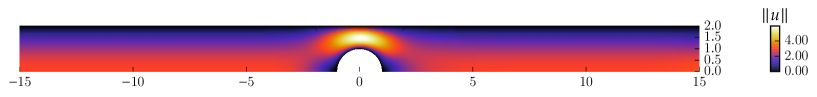
Figure 8: Flow field for mesh “$48$” with automatically created matrix.

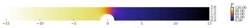
Figure 9: Pressure field for mesh “$48$” with automatically created matrix.

Some performance issues that arise from the automatic creation of the matrix were mentioned in Section 3.2, along with one possibility for mediating some of these effects. Table 1 shows how much time the calculation of the left- and right-hand sides takes up for some different mesh resolutions, when the matrix is created by different means. In agreement with the predictions that were made in Section 3.2, the execution of the matrix calculation code created by automatic differentiation takes much longer than that of the manually created code. The ratio between both execution times varies considerably for the different simulations. When the execution time of the optimized AD code—with separate input vectors for all degrees of freedom, as described in Section 3.2—is compared with that of the unoptimized AD code, the difference between the simulations is much less pronounced. The optimized code reliably outperforms the unoptimized code, with a performance gain of around $46\%$.

Method	Mesh 48	Mesh 96	Mesh 192	Mesh 384	Mesh 768
manual derivative	0.98 s	1.69 s	3.37 s	6.63 s	13.05 s
unoptimized automatic derivative	13.27 s	26.48 s	52.76 s	105.73 s	210.28 s
separation by degree of freedom	7.04 s	14.33 s	28.36 s	57.24 s	113.62 s
number of processors	16	32	64	128	256

Table 1: Time taken up by matrix calculations for different methods (rows) and meshes (columns) with $Wi=0.05$.

These times can be put into perspective when they are compared to the total execution times of the simulation. Table 2 shows the percentage of the total execution time which is taken up by the left- and right-hand side accumulations in the different cases. Again, these numbers differ enormously when the different simulations are compared. With every increase in the number of processors, the percentage decreases. This suggests that the matrix accumulation code scales much better than the linear solver code. The performance losses incurred by the method may therefore become negligible for some realistic problems. However, the numbers in the first two columns show that the influence can become very large in certain cases. This confirms the assumption that the optimization of the automatic differentiation method remains an important and necessary task.

Method	Mesh 48	Mesh 96	Mesh 192	Mesh 384	Mesh 768
manual derivative	4.5 %	3.5 %	1.9 %	0.8 %	0.3 %
unoptimized automatic derivative	40.5 %	36.8 %	21.0 %	10.5 %	4.5 %
separation by degree of freedom	30.2 %	25.7 %	13.5 %	6.4 %	2.5 %

Table 2: Time taken up by matrix calculations for different methods and meshes, given as percentage of total execution time.

We want to look at the efficiency of the differentiated code more closely. The evaluation of a function resulting from forward mode automatic differentiation always includes the evaluation of the original function. Therefore, we can assume the computational cost of such an evaluation to be $1+\alpha$ times greater than the cost of the original function evaluation, with positive $\alpha$. If the same function is used as the basis for vector forward mode, with $p$ directional derivatives being evaluated simultaneously, we can assume the cost ratio to be $1+\alpha\cdot p$.

In [29, §4.5], it is shown that the upper bound for $\alpha$ is $1.5$ in this case. For comparison, a finite-difference approach would yield $\alpha=1$. For our example, when comparing actual execution times, we could achieve values of $\alpha$ between $2.18$ and $2.27$ for the unoptimized approach, and values between $1.14$ and $1.23$ for the optimized approach, with separated degrees of freedom.

The values for the unoptimized approach may seem unrealistic at first, when compared to the upper bound given in [29]. However, we would like to point out that these execution times depend greatly on issues such as compiler optimization, cache handling, etc., and that the loss in efficiency may also partially result from the increased memory requirements of the differentiated function.

One interesting result is that even our optimized approach is still less efficient than a one-sided finite-difference approach. Nonetheless, one should note that this slight increase in execution time comes with the bonus of a much more accurate derivative, and removes the necessity of having to choose a suitable step size.

5 Conclusion

The objective of this work was to simplify the implementation of partial differential equations into finite element codes. This was attempted by using automatic differentiation for the creation of the code for the calculation of the Jacobian matrix. As the results of the test case in the previous section prove, a useful method for this purpose could indeed be developed. However, during the development of this method, several problems surfaced that could not be solved in a universal manner. In these cases, the solutions were specific to the program code and equations at hand, and would need to be adjusted to be useful in different contexts.

One of these problems lies in TAPENADE’s incomplete support of the Fortran programming language. Even though we used a source code that works perfectly with the popular Fortran compilers, many changes were necessary in order to make it work with TAPENADE. Some of these changes could be automated, but it is to be expected that other source codes will bring to light further problems of this nature. The complexity of the changes that would need to be automated to support arbitrary Fortran codes is in fact of such magnitude that only a program equipped with a full-featured Fortran parser could reliably do the job.

TAPENADE incorporates a feature that is useful for the automatic creation of full Jacobian matrices instead of single directional derivatives. This is its vector mode for the simultaneous calculation of arbitrary numbers of directional derivatives of the same function. This is a step in a good direction and paves the way for some important optimizations. However, the resulting code can generally be expected to be less efficient than a well thought-out manual implementation. The closed-source nature of TAPENADE means that any further optimization techniques either have to be applied manually or require a separate language parser. Exploiting sparsity in input vectors or other properties of the code structure therefore involves a significant amount of additional work.

One important finding of the present work is the fact that the special structure of the finite element method allows for an easy automatic creation of a huge Jacobian matrix with full exploitation of the matrix sparsity by combining the typical finite element assembly process with automatic differentiation on the element level (see Section 3.1). The final step on the path towards a method that will be ready for production use will now lie in the combination of this code design with more efficient methods for the automatic creation of the dense element-level matrix (see Section 3.2 for some approaches leading in this direction). As shown in Section 4.4, we already achieved significant efficiency improvements with a first optimization attempt.

The developments described in this document had the side effect of prompting the discovery and resolution of a number of incompatibilities between TAPENADE and current Fortran standards (see Section 2.2). The knowledge that was gained this way will aid considerably in the implementation of further projects involving TAPENADE, that go beyond the calculation of Jacobian matrices.

6 Acknowledgements

The authors gratefully acknowledge the support of DFG under the collaborative research project SFB 1120 (subproject B2) and DFG grant ”Computation of Die Swell Behind a Complex Profile Extrusion Die Using a Stabilized Finite Element Method for Various Thermoplastic Polymers”.

References

- [1] T. J. Ypma, Historical development of the Newton-Raphson method, SIAM review 37 (4) (1995) 531–551.
- [2] Y. Saad, M. Schultz, GMRES: A generalized minimal residual algorithm for solving nonsymmetric linear systems, SIAM Journal on Scientific and Statistical Computing 7 (3) (1986) 856–869.
- [3] P. D. Hovland, L. C. McInnes, et al., Parallel simulation of compressible flow using automatic differentiation and PETSc, Parallel Computing 27 (4) (2001) 503–519.
- [4] J. Brown, Efficient nonlinear solvers for nodal high-order finite elements in 3D, Journal of Scientific Computing 45 (1-3) (2010) 48–63.
- [5] A. Curtis, M. J. Powell, J. K. Reid, On the estimation of sparse Jacobian matrices, J. Inst. Math. Appl 13 (1) (1974) 117–120.
- [6] G. Kedem, Automatic differentiation of computer programs, ACM Transactions on Mathematical Software (TOMS) 6 (2) (1980) 150–165.
- [7] A. Griewank, et al., On automatic differentiation, Mathematical Programming: recent developments and applications 6 (6) (1989) 83–107.
- [8] H. M. Bücker, M. Lülfesmann, Combinatorial optimization of stencil-based jacobian computations, in: Proceedings of the 2010 International Conference on Computational and Mathematical Methods in Science and Engineering, Almería, Andalucía, Spain, Vol. 1, 2010, pp. 284–295.
- [9] D. R. Reynolds, R. Samtaney, Sparse jacobian construction for mapped grid visco-resistive magnetohydrodynamics, in: Recent Advances in Algorithmic Differentiation, Springer, 2012, pp. 11–21.
- [10] A. Griewank, S. Reese, On the calculation of Jacobian matrices by the Markowitz rule, Tech. rep., Argonne National Lab., IL (United States) (1991).
- [11] A. Griewank, Direct calculation of Newton steps without accumulating Jacobians, Large-scale numerical optimization (1990) 115–137.
- [12] T. F. Coleman, A. Verma, The efficient computation of sparse Jacobian matrices using automatic differentiation, SIAM Journal on Scientific Computing 19 (4) (1998) 1210–1233.
- [13] U. Naumann, Optimal Jacobian accumulation is NP-complete, Mathematical Programming 112 (2) (2008) 427–441.
- [14] C. Bischof, A. Griewank, ADIFOR: A Fortran system for portable automatic differentiation, Preprint MCS-P317-0792 (Mathematics and Computer Science Division, Argonne National Laboratory, Argonne, Illinois, 1992).
- [15] C. Bischof, A. Carle, G. Corliss, A. Griewank, P. Hovland, ADIFOR–generating derivative codes from Fortran programs, Scientific Programming 1 (1) (1992) 11–29.
- [16] N. Rostaing, S. Dalmas, A. Galligo, Automatic differentiation in Odyssee, Tellus A 45 (5) (1993) 558–568.
- [17] L. Hascoët, V. Pascual, The Tapenade Automatic Differentiation tool: Principles, Model, and Specification, ACM Transactions On Mathematical Software 39 (3) (2013) 1–50.
- [18] J. Utke, U. Naumann, M. Fagan, N. Tallent, M. Strout, P. Heimbach, C. Hill, C. Wunsch, OpenAD/F: A modular open-source tool for automatic differentiation of Fortran codes, ACM Transactions on Mathematical Software (TOMS) 34 (4) (2008) 18.
- [19] J.-F. Barthelemy, L. E. Hall, Automatic differentiation as a tool in engineering design, Structural optimization 9 (2) (1995) 76–82.
- [20] G. F. Corliss, A. Griewank, Operator overloading as an enabling technology for automatic differentiation, Tech. rep., Argonne National Lab., IL (United States). Funding organisation: USDOE, Washington, DC (United States) (1993).
- [21] M. Tadjouddine, S. A. Forth, J. D. Pryce, AD tools and prospects for optimal AD in CFD flux Jacobian calculations, in: Automatic differentiation of algorithms, Springer, 2002, pp. 255–261.
- [22] S. A. Forth, M. Tadjouddine, J. D. Pryce, J. K. Reid, Jacobian code generated by source transformation and vertex elimination can be as efficient as hand-coding, ACM Transactions on Mathematical Software (TOMS) 30 (3) (2004) 266–299.
- [23] F. Smailbegovic, G. Gaydadjiev, S. Vassiliadis, Sparse matrix storage format, in: Proceedings of the 16th Annual Workshop on Circuits, Systems and Signal Processing, ProRisc 2005, 2005, pp. 445–448.
- [24] P. Knechtges, M. Behr, S. Elgeti, Fully-implicit log-conformation formulation of constitutive laws, Journal of Non-Newtonian Fluid Mechanics 214 (2014) 78–87. arXiv:1406.6988, doi:10.1016/j.jnnfm.2014.09.018.
- [25] P. Knechtges, The fully-implicit log-conformation formulation and its application to three-dimensional flows, Journal of Non-Newtonian Fluid Mechanics 223 (2015) 209–220. arXiv:1503.03863, doi:10.1016/j.jnnfm.2015.07.004.
- [26] R. Fattal, R. Kupferman, Constitutive laws for the matrix-logarithm of the conformation tensor, Journal of Non-Newtonian Fluid Mechanics 123 (2) (2004) 281–285.
- [27] C. Moler, C. Van Loan, Nineteen Dubious Ways to Compute the Exponential of a Matrix, Twenty-Five Years Later, SIAM Review 45 (1) (2003) 3–49.
- [28] T. Kato, Perturbation Theory for Linear Operators, Springer-Verlag, 1995.
- [29] A. Griewank, A. Walther, Evaluating Derivatives: Principles and Techniques of Algorithmic Differentiation, Society for Industrial and Applied Mathematics, 2008.