Checks of integrality properties
in topological strings

Abstract

Tests of the integrality properties of a scalar operator in topological strings on a resolved conifold background or orientifold of conifold backgrounds have been performed for arborescent knots and some non-arborescent knots. The recent results on polynomials for those knots colored by $SU(N)$ and $SO(N)$ adjoint representations [1] are useful to verify Marino’s integrality conjecture up to two boxes in the Young diagram. In this paper, we review the salient aspects of the integrality properties and tabulate explicitly for an arborescent knot and a link. In our knotebook website, we have put these results for over 100 prime knots available in Rolfsen table and some links. The first application of the obtained results, an observation of the Gaussian distribution of the LMOV invariants is also reported.

^a Lebedev Physics Institute, Moscow 119991, Russia
^b ITEP, Moscow 117218, Russia
^c Institute for Information Transmission Problems, Moscow 127994, Russia
^d Laboratory of Quantum Topology, Chelyabinsk State University, Chelyabinsk 454001, Russia
^e Department of Physics, Indian Institute of Technology Bombay, Mumbai 400076, India

1 Introduction

Topological string duality conjectures put forth by Gopakumar-Vafa [2] and Ooguri-Vafa [3] relates $U(N)$ Chern-Simons theory on $S^{3}$ to topological string theory on resolved conifold. This has led to rewrite suitable combinations of Chern-Simons knot polynomials [4, 5, 6] as reformulated invariants possessing integrality structures [7, 28, 8, 9, 10] famously known as LMOV condition (see also [11] for the latest development). These integer invariants count the BPS states(spectra of M2 branes ending on M5 branes in M-theory compactified on the conifold [2]). These integers determine the oriented topological string amplitudes. The challenge to obtain the integers needs polynomial form of unreduced colored HOMFLY-PT for any knot/link. In fact, a recent breakthrough [12]-[23],[1] enabled evaluation of colored HOMFLY-PT polynomials. Our knotebook website [24] which gets updated periodically gives the list of knots for which polynomials are obtained. Thus we can indirectly determine the BPS integers for such knots and thus verify the integrality structures within topological string duality context.

The LMOV [3, 10] integrality condition is much stronger than the integrality of colored HOMFLY-PT and Kauffman knot polynomials. That is, in suitable variables ($q=\exp\left(\frac{2\pi i}{k+N}\right)$ and $A=q^{N}$), the expectation values of Wilson loop operators

$$P^{\cal L}_{R}(A,q)\ =\ \left<{\rm Tr}_{R}\ T\exp\left(\oint_{\cal L}{\cal A}\right)\right>$$ (1)

in $SU(N)$(colored HOMFLY-PT) or $SO(N+1)$ (colored Kauffman) Chern-Simons theories are Laurent polynomials with integer coefficients. There was no topological arguments to justify these integers. The categorification technique introduced by Khovanov-Rozansky [25] interprets these integers as dimension of doubly graded vector space. It is still a challenging question to find the connection of such a categorification approach and the conventional Reshetikhin-Turaev (RT) formalism [26]-[35]. In refs. [36, 37, 38], these integers in Jones polynomials are interpreted as counting solutions of Hitchin equation in a four dimensional gauge theory for a given instanton number.

There is an elegant way of writing expectation value of Ooguri-Vafa scalar operator for knots in topological strings [3] using plethystic exponential of a spectrum generating function (SGF) known as index. Technically, if a Hilbert space has a SGF

$$Ind_{H}(t)=\sum_{i}\tilde{N}_{i}t^{i}~{},$$ (2)

then, the Fock space has a single state (vacuum) at the zeroth level, $M_{1}=\tilde{N}_{1}$ states at the first level, $M_{2}=\tilde{N}_{2}+\frac{1}{2}\tilde{N}_{1}(\tilde{N}_{1}+1)$ states at the second level, $M_{3}=\tilde{N}_{3}+\tilde{N}_{2}\tilde{N}_{1}+\frac{1}{6}\tilde{N}_{1}(\tilde{N}_{1}+1)(\tilde{N}_{1}+1)$ at the third, and so on, and the SGF in the Fock space is the plethystic exponential of “the free energy” (of SGF) in the Hilbert space:

$$Ind_{F}(t)=\sum_{I}M_{I}t^{I}=\prod_{i}\frac{1}{(1-t^{i})^{\tilde{N}_{i}}}=\exp\sum_{d=1}\frac{Ind_{H}(t^{d})}{d}$$ (3)

Thus, if some quantity is supposed to have an interpretation as an SGF, its plethystic logarithm should also resemble an SGF: possess integrality properties. The original Ooguri-Gopakumar-Vafa conjecture [2, 3] for knot polynomials reflected the old belief that they are actually characters, and the plethysm operation is well known to act naturally on the characters [39] (physically the plethysm operation in the conjecture is related with the Schwinger mechanism of brane creation [2]). For example, the generating function of quantum dimensions (in knot theory these are unreduced HOMFLY polynomials for the unknot) is

$$Z_{OV}^{unknot}\{A,q\,|\,\bar{p}\}=\sum_{R}{\rm dim}_{{}_{R}}(A,q)\cdot\chi_{R}\{\bar{p}\}=\sum_{R}\chi_{R}(p^{*})\chi_{R}(p)=\exp\left(\sum_{d}\frac{p_{d}^{*}\bar{p}_{d}}{d}\right)=$$

$$=\exp\left(\sum_{d}\frac{1}{d}\widehat{Ad}_{d}(p_{1}^{*})\,\widehat{Ad}_{d}(\bar{p}_{1})\right)=\exp\left(\sum_{d}\frac{p_{1}^{*}(A^{d},q^{d})}{d}\,\widehat{Ad}_{d}(\bar{p}_{1})\right)~{},$$ (4)

where the sum runs over all Young diagrams $R$ (“colors”), $\chi_{R}$ are the Schur functions of time variables $\bar{p}_{k}$ and the Adams (plethysm) operation $\ \widehat{Ad}_{d}:\ p_{k}\longrightarrow p_{kd}$ acts at the topological locus [31, 40] by raising the power of parameters:

$$\widehat{Ad}_{d}(p_{k}^{*})=p^{*}_{kd}=\frac{A^{kd}-A^{-kd}}{q^{kd}-q^{kd}}=p_{k}^{*}(A^{d},q^{d})~{}.$$ (5)

The plethystic logarithm of $Z_{OV}^{unknot}$ is therefore $p_{1}^{*}=\frac{A-A^{-1}}{q-q^{-1}}$ and it possesses the integrality property:

$$(q-q^{-1})\cdot p_{1}^{*}=A-A^{-1}$$ (6)

is a Laurent polynomial in variables $A$ and $q$ with integer coefficients for any knot. In this case of unknot, it is actually independent of $q$. The claim is that such an integrality property is true for plethystic logarithms for the Ooguri-Vafa generating functions of colored HOMFLY for all knots. In particular, it suggests that free energies have only the first order poles in the Planck constant $\hbar=\log q$ which is expected for the partition function but not so obvious for unreduced knot polynomials ( $P_{R}\sim\hbar^{-|R|}$).

As follows from (4), the plethystic transform exactly compensates the deviation, of the dimension $d_{R}$ from $\frac{d_{1}^{|R|}}{|R|!}$ (both classical and quantum dimensions). Further the deviation of the HOMFLY polynomial of general knots from the quantum dimension, i.e. non-classical nature of cabling, is measured by the Ooguri-Vafa polynomials $f_{R}$(reformulated invariants). Basically, these are homogeneous polylinear combinations

$$f_{R}=H_{R}+\sum_{I}c_{I}\prod_{i\in I}\widehat{Ad}_{n_{i}}\!\big{(}H_{R_{i}}\big{)}$$ (7)

with $\sum_{i}n_{i}|R_{i}|=|R|$ and all $|R_{i}|<|R|$, which vanish if all HOMFLY polynomials are substituted by the dimensions, $H_{R}\longrightarrow d_{R}$, e.g. $f_{[2]}=H_{[2]}-\frac{1}{2}H_{[1]}^{2}-\frac{1}{2}\widehat{Ad}_{2}(H_{1})$. This property defines them up to triangular transforms, and they automatically have only the first-order poles in $\{q\}(=q-q^{-1})$.

While similarity between knot polynomials and characters of an infinite-dimensional algebra is still a plausible conjecture (see some examples in [41]), the fact is that these averages(1) for arbitrary representations involves character decomposition. Further localization ideas a la [42, 43, 44, 45, 46] can convert these averages into a finite-dimensional matrix model integral satisfying the AMM/EO topological recursion [47]. This has been achieved for the torus knots [48]. There are still difficulties implementing AMM/EO topological recursion for twist knots [49] but there is some evidence of applicability of AMM/EO recursion to the non-torus knot $4_{1}$ [50].

Motivated by the t’Hooft large $N$ genus expansion (closed string partition function) for free energies in gauge theories, we do expect genus expansion in $\hbar$ at fixed t’ Hooft coupling ($A$ fixed) for logarithm of the colored HOMFLY polynomials $\ln H_{R}^{\cal K}(A,q)$. There is an alternative genus expansion [51] known as Hurwitz-Fourier transform in variable $\mathfrak{h}$:

$$H_{R}^{\cal K}(A,q)=\hbox{dim}_{R}(A,q)\cdot\Big{(}\sigma_{{}_{\Box}}^{\cal K}(A)\Big{)}^{|R|}\cdot\exp\left(\sum_{\Delta}\mathfrak{h}^{|\Delta|+l(\Delta)-2}s_{\Delta}^{\cal K}(A,\mathfrak{h}^{2})\varphi_{R}(\Delta)\right)\ \ \ \ \ \ \ \ \ \mathfrak{h}={\hbar\over\Big{(}\sigma_{{}_{\Box}}^{\cal K}(A)\Big{)}^{2}}$$ (8)

where $\sigma_{{}_{\Box}}^{\cal K}(A)=H^{\cal K}_{\Box}(q=1,A)$ are called special polynomials. This expansion results in the appearance of Hurwitz-Tau function when substituted in the Ooguri-Vafa partition function $Z_{OV}^{\cal K}(A,q,\bar{p})$ [52, 53]. Here the sum goes over the Young diagrams $\Delta$ with $l(\Delta)$ lines of lengths $\delta_{i}$ and the number of boxes $|\Delta|=\sum_{i}^{l(\Delta)}\delta_{i}$, while $\varphi_{R}(\Delta)$ are proportional to the characters of symmetric groups $\psi_{R}(\Delta)$ at $|R|=|\Delta|$: $\psi_{R}(\Delta)=z_{\Delta}d_{R}\varphi_{R}(\Delta)$, and continued to $|R|>|\Delta|$ as in [52, eq.(3)]. Here $d_{R}$ is the dimension of representation $R$ of the symmetric group $S_{|R|}$ divided by $|R|!$ and $z_{\Delta}$ is the standard symmetric factor of the Young diagram (order of the automorphism) [54]. With this definition, the sum in (8) runs over all $\Delta$ such that $|\Delta|\leq|R|$, while in all sums below we use $\psi_{R}(\Delta)$ which leaves in sums only terms with $|R|=|\Delta|$. An advantage to use the expansion (8) is in a possibility of lifting $\varphi_{R}(\Delta)$ to a ring of cut-and-join operators $W_{\Delta}$ [52], while using the basis of $\psi_{R}(\Delta)$ is better for studying integrality conjectures.

This Hurwitz version of the Fourier transform in the color index $R$, (8) converts the set of colored HOMFLY polynomials into a collection of generalized special polynomials $\sigma_{g|\Delta}^{\cal K}(A)$ [51]. They enter (8) through

$$s_{\Delta}^{\cal K}(A,\mathfrak{h}^{2})=\sum_{g\geq 0}\mathfrak{h}^{2g}\sigma_{g|\Delta}^{\cal K}(A)$$ (9)

Note that the free energy behaves as $\hbar^{-2}$, which is natural for $\tau$-functions.

The properties of this genus/Hurwitz expansion of individual knot polynomials did not yet gain enough attention. However, eq.(8) calls for study of the genus expansion of the Ooguri-Vafa partition functions and implies that a natural form for it should involve the plethystic exponential:

$$Z_{OV}^{\cal K}\{A,q\,|\,\bar{p}\}=\sum H_{R}^{\cal K}(A,q)\chi_{R}\{\bar{p}\}=\exp\left(\sum_{d\geq 1}\sum_{\Delta}\frac{\prod_{i=1}^{l(\Delta)}(q^{d\delta_{i}}-q^{-d\delta_{i}})}{d}\,S_{\Delta}^{\cal K}\ (A^{d},q^{d})\widehat{Ad}_{d}(\bar{p}_{\Delta})\right)$$ (10)

where $\bar{p}_{\Delta}=\prod_{i}\bar{p}_{i}^{\,\mu_{i}}$ and $\ \widehat{Ad}_{d}(\bar{p}_{\Delta})=\prod_{i}\bar{p}_{di}^{\,\mu_{i}}$, where $\mu_{i}$ is equal to the number of times that the line of length $i$ is met in the Young diagram $\Delta$. In these terms, $z_{\Delta}=\prod_{i}i^{\mu_{i}}\mu_{i}!$ .

Relation between (10) and (8) is not at all naive, since the sum of logarithm is not equal to a logarithm of the sum, or the sum of genus expansions is not the same as a genus expansion of the sum. It involves generalizations of the Cauchy formula (4) to the generation function of the generalized Hurwitz numbers [55, 56, 52]

$$Z_{OV}^{\cal K}\{A,q\,|\,\bar{p}\}\equiv Z_{Hurw}=\sum_{R}{\rm dim}_{{}_{R}}(A,q)\cdot\chi_{R}\{\bar{p}\}\cdot e^{\sum_{\Delta}\beta_{\Delta}\varphi_{R}(\Delta)}$$ (11)

where $\beta_{\Delta}$ encodes knot ${\cal K}$ information. The $\varphi_{R}(\Delta)$ appears in the “multipoint ”correlators” of generalized symmetric group characters as follows:

$${\rm Hurw}_{q}(\Delta_{1},\Delta_{2},\ldots,\Delta_{m})=\sum_{|R|=q}d_{R}^{2}\varphi_{R}(\Delta_{1})\varphi_{R}(\Delta_{2})\ldots\varphi_{R}(\Delta_{m})$$ (12)

Note that (10) uses yet another different version of genus expansion, that is., in power of $q-q^{-1}$ rather than $\hbar$ [51]. One can rewrite the product

$${\prod_{i=1}^{l(\Delta)}(q^{d\delta_{i}}-q^{-d\delta_{i}})}={\prod_{j=1}(q^{jd}-q^{-jd})^{\mu_{j}}}$$ (13)

which resembles the measure for the $\beta$-ensemble [57]: $(x_{1}-x_{2})^{\beta}\longrightarrow\prod_{i=0}^{\beta-1}(x_{1}-q^{2i}x_{2})$. One can also look at it as a product of $q$-numbers $[\delta_{i}]_{q^{d}}$ or $[j]_{q^{d}}^{\mu_{j}}$, which generates an additional factor of $(q^{d}-q^{-d})^{l(\Delta)}$. Hence, the additional suppression $\hbar^{|\Delta|}$ in (8) disappears from (10).

The LMOV integrality conjecture claims that after one more Hurwitz transform of $S_{\Delta}(q,A)$ in (10),

$$S_{\Delta}(q,A)=\sum_{Q}\psi_{Q}(\Delta)\cdot G_{Q}(A,q)$$ (14)

the genus expansions

$$G_{Q}(A,q)=\sum_{g\geq 0,k}N_{Q,g,k}A^{k}(q-q^{-1})^{2g-2}$$ (15)

have integer coefficients. Moreover, integers $N_{Q,g,k}$ at fixed $Q$ and $k$ actually vanish at high enough genus $g$, this is an advantage of the above mentioned invariant version of the expansion. This LMOV integrality of every term of the genus expansion is, of course, much stronger than just integrality of the entire free energy.

Note that relation (14) can be immediately inverted:

$$G_{Q}(A,q)=\sum_{\Delta}{1\over z_{\Delta}}\psi_{Q}(\Delta)S_{\Delta}(q,A)$$ (16)

due to the orthogonality conditions

$$\sum_{R}{1\over z_{\Delta}}\psi_{R}(\Delta)\psi_{R}(\Delta^{\prime})=\delta_{\Delta\Delta^{\prime}},\ \ \ \ \ \sum_{\Delta}{1\over z_{\Delta}}\psi_{R}(\Delta)\psi_{R^{\prime}}(\Delta)=\delta_{RR^{\prime}}$$ (17)

An important implication of the Hurwitz approach is that $Z_{OV}\{\bar{p}\}$ should satisfy the AMM/OE topological recursion in $g$, and this fact was actually used in the study of proofs of LMOV relation in [61]. Such studies have not be extended to prove Marino’s integrality conjectures involving Kauffman polynomials which we hope to pursue in future.

It is appropriate to mention that Marino’s conjectures have been verified for some torus knots and links [62, 63, 64] and figure-eight knot [65]. Hence the main focus in this paper is to verify Marino’s integrality conjectures for various arborescent knots up to 8 crossings using colored Kauffman polynomials ($SO(N)$ colors up to two boxes in Young diagram) and HOMFLY polynomials for mixed $SU(N)$ representations. The latter are calculated using the universal Racah matrices [1] which are known only for the arborescent knots.

Informally, arborescent knots are the ones which look like trees with two-bridge branches, i.e. by gluing together the fragments of 4-strand antiparallel braids, see [17], where they were named double-fat. This is what makes their knot polynomials expressible through the two simplest Racah matrices ${\cal S}$ and $\bar{\cal S}$ (see s.3.5 below). They are also well familiar in formal knot theory, see [6, 66] for an abstract definition and other details. The list of arborescent knots includes, in particular, all twisted, 2-bridge and pretzel knots. This means that all prime knots with up to 7 intersections are arborescent being 2-bridge. Among the knots with 8 crossings the only non-arborescent prime knot is $8_{18}$. Moving further in the Rolfsen table, among the knots with 9 crossings, only $9_{34}$, $9_{39}$, $9_{40}$, $9_{41}$, $9_{47}$, $9_{49}$ are non-arborescent. At last, among the knots with 10 crossings, $10_{100}$–$10_{123}$ and $10_{155}$–$10_{165}$ are non-arborescent (polyhedral).

We will also present the LMOV integrality structures for $SU(N)$ colors up to four boxes in the Young diagram as well. It allows us to reveal a striking feature of the LMOV numbers: it turns out that, with a very high accuracy, the LMOV numbers appeared to be distributed by a Gaussian law as functions of the genus $g$! It is just an observation that has been tested for various knots, and no exception has been found so far.

In sec.2, we review the exact formulation of the integrality conjectures. In sec.3, we briefly recapitulate the recent progress in knot polynomial calculus. In sec.4, we will present in detail the integrality checks for a particular knot and link. We refer the reader to our dedicated site [24] where the results for other knots are updated. In sec.5, we report on the first application of the obtained results: the Gaussian distribution of the LMOV invariants. In the concluding sec.6, we summarize the results obtained.

2 LMOV conjecture: integrality conditions

2.1 Integrality conjecture in the HOMFLY case

As we explained in the introduction section, the genus expansion in knot theory is determined using gauge/string duality [2, 3]. That is, $U(N)$ Chern-Simons theory on a three-manifold $S^{3}$ is equivalent to topological string theory on a Calabi-Yau manifold which is the resolution of the conifold. The expectation value of the Ooguri-Vafa scalar operator associated with knots in $S^{3}$,

$${\cal Z}_{SU(N)}^{\cal K}\{A,q\,|\,\bar{p}\}=\sum_{R}H_{R}^{\cal K}(A,q)\cdot\chi_{R}\{\bar{p}\}$$ (18)

which is a generating function of the unreduced HOMFLY polynomials $H_{R}^{\cal K}(A,q)$, results in $A$-model open topological string partition function. In fact the logarithm of the operator can be interpreted as “connected” correlators $f_{R}(q,A)$ as follows:

$$\log{\cal Z}^{\cal K}_{SU}\{A,q|\bar{p}\}=\sum_{R}\sum_{d=1}^{\infty}\,\frac{1}{d}{f}_{R}^{\cal K}(A^{d},q^{d})\cdot\widehat{Ad}_{d}\,\chi_{R}\{\bar{p}\}$$ (19)

We call the new quantities $f_{R}$ plethystic transforms of the adjoint HOMFLY polynomials by the reasons explained in the introduction section. Note that, the relation (14) can be inverted leading to constructing the inverse of plethysm transformation as performed in [9]:

$$f_{R}^{\cal K}(A,q)=\sum_{d,m=1}(-1)^{m-1}{\mu(d)\over md}\sum_{\Delta_{1},\ldots\Delta_{m}}\widehat{Ad}_{d}\,\psi_{R}\Big{(}\sum_{i=1}^{m}\Delta_{i}\Big{)}\cdot\sum_{R_{1},\ldots,R_{m}}\prod_{j=1}^{m}{\psi_{R_{j}}(\Delta_{j})\over z_{\Delta_{j}}}H_{R_{j}}^{\cal K}(A^{d},q^{d})$$ (20)

where the sum of two Young diagrams $\Delta$ and $\Delta^{\prime}$ is the Young diagram with the lines $\{\delta_{i},\delta_{i}^{\prime}\}$ with a proper reordering, $\widehat{Ad}_{d}\,\Delta=\widehat{Ad}_{d}\,\{\delta_{i}\}=\{d\delta_{i}\}$, and $\mu(d)$ is the Möbius function defined as follows: if the prime decomposition of $d$ consists of $m$ multipliers and contains non-unit multiplicities, $\mu(d)=0$, otherwise $\mu(d)=(-1)^{m}$. For representations up to four boxes in Young diagram, the explicit form of the above equation will be

$$f_{[1]} = H_{[1]}(q,A)$$

$$f_{[2]} = H_{[2]}(q,A)-{1\over 2}\Big{(}H_{[1]}(q,A)^{2}+H_{[1]}(q^{2},A^{2})\Big{)}$$

$$f_{[1^{2}]} = H_{[1^{2}]}(q,A)-{1\over 2}\Big{(}H_{[1]}(q,A)^{2}-H_{[1]}(q^{2},A^{2})\Big{)}$$

$$f_{[3]} = H_{[3]}-H_{[2]}H_{[1]}+\frac{1}{3}H_{[1]}^{3}-\frac{1}{3}H_{[1]}(A^{3},q^{3})$$

$$f_{[2,1]} = H_{[2,1]}-H_{[2]}H_{[1]}-H_{[1^{2}]}H_{[1]}+\frac{2}{3}H_{[1]}^{3}-\frac{1}{3}H_{[1]}(A^{3},q^{3})$$

$$f_{[1^{3}]} = H_{[1^{3}]}-H_{[1^{2}]}H_{[1]}+\frac{1}{3}H_{[1]}^{3}-\frac{1}{3}H_{[1]}(A^{3},q^{3})$$

$$f_{[4]} = H_{[4]}-H_{[3]}H_{[1]}+H_{[2]}H_{[1]}^{2}-\frac{1}{2}H_{[2]}^{2}-\frac{1}{4}H_{[1]}^{4}-\frac{1}{2}H_{[2]}(A^{2},q^{2})+\frac{1}{4}H_{[1]}^{2}(A^{2},q^{2})$$

$$f_{[3,1]} = H_{[3,1]}-H_{[3]}H_{[1]}-H_{[2,1]}H_{[1]}-H_{[2]}H_{[1^{2}]}+2H_{[2]}H_{[1]}^{2}+H_{[1^{2}]}H_{[1]}^{2}-\frac{1}{2}H_{[2]}^{2}-\frac{3}{4}H_{[1]}^{4}+\frac{1}{2}H_{[2]}(A^{2},q^{2})-\frac{1}{4}H_{[1]}^{2}(A^{2},q^{2})$$

$$f_{[2^{2}]} = H_{[2^{2}]}-H_{[2,1]}H_{[1]}+H_{[2]}H_{[1]}^{2}+H_{[1^{2}]}H_{[1]}^{2}-\frac{1}{2}H_{[2]}^{2}-\frac{1}{2}H_{[1^{2}]}^{2}-\frac{1}{2}H_{[1]}^{4}-\frac{1}{2}H_{[2]}(A^{2},q^{2})-\frac{1}{2}H_{[1^{2}]}(A^{2},q^{2})+\frac{1}{2}H_{[1]}^{2}(A^{2},q^{2})$$

$$f_{[2,1^{2}]} = H_{[2,1^{2}]}-H_{[1^{3}]}H_{[1]}-H_{[2,1]}H_{[1]}-H_{[2]}H_{[1^{2}]}+2H_{[1^{2}]}H_{[1]}^{2}+H_{[2]}H_{[1]}^{2}-\frac{1}{2}H_{[2]}^{2}-\frac{3}{4}H_{[1]}^{4}+\frac{1}{2}H_{[1^{2}]}(A^{2},q^{2})-\frac{1}{4}H_{[1]}^{2}(A^{2},q^{2})$$

$$f_{[1^{4}]} = H_{[1^{4}]}-H_{[1^{3}]}H_{[1]}+H_{[1^{2}]}H_{[1]}^{2}-\frac{1}{2}H_{[1^{2}]}^{2}-\frac{1}{4}H_{[1]}^{4}-\frac{1}{2}H_{[2]}(A^{2},q^{2})+\frac{1}{4}H_{[1]}^{2}(A^{2},q^{2})$$

Now, the expansion of HOMFLY polynomial is translated into a similar expansion of the plethystic polynomials:

$$f_{R}(q,A)=\sum_{n,k}\widetilde{\bf N}_{R,n,k}{A^{n}q^{k}\over q-q^{-1}}$$ (21)

Even though HOMFLY behaves as $1/(q-q^{-1})^{|R|}$, the reformulated invariant $f_{R}(q,A)$ has only singularity $1/(q-q^{-1})$

In fact, the only way to check this duality between Chern-Simons and topological string theories is to establish the integrality condition: the coefficients $\widetilde{\bf N}_{R,n,k}$ has to be integer in accordance with the Ooguri-Vafa conjecture [3]. Moreover, as we explained in the introduction section, one can construct even more refined integers (14) [8]

$$f_{R}(q,A)=\sum_{n,k\geq 0,Q}C_{RQ}{\bf N}_{Q,n,k}A^{n}(q-q^{-1})^{2k-1}$$ (22)

where

$$C_{RQ}=\sum_{\Delta}{1\over z_{\Delta}}\psi_{R}(\Delta)\psi_{Q}(\Delta){\prod_{i=1}^{l(\Delta)}\Big{(}q^{\delta_{i}}-q^{-\delta_{i}}\Big{)}\over q-q^{-1}}={1\over q-q^{-1}}\sum_{\Delta}{1\over z_{\Delta}}\psi_{R}(\Delta)\psi_{Q}(\Delta)\ ^{*}p_{\Delta}$$ (23)

with ${}^{*}p_{k}\equiv q^{k}-q^{-k}$. To compare this formula with (14), one has to use the identity

$$\sum_{R}\psi_{R}(\Delta)\chi_{R}(p)=p_{\Delta}$$

This matrix can be easily reversed using (17):

$$\Big{(}C^{-1}\Big{)}_{QR}=\sum_{\Delta}{1\over z_{\Delta}}\psi_{R}(\Delta)\psi_{Q}(\Delta){q-q^{-1}\over{}^{*}p_{\Delta}}$$ (24)

Let us note that there is a hierarchy of integralities: the weakest statement is the claim that the HOMFLY polynomials are integer. The next level is integrality of $\widetilde{\bf N}_{R,n,k}$, which implies that of HOMFLY, but not vice versa. However, $\widetilde{\bf N}_{R,n,k}$ are not independent: they satisfy some relations [7], while the more refined ${\bf N}_{R,n,k}$ are independent numbers and their integrality implies the integrality of $\tilde{\bf N}_{R,n,k}$, but not vice versa. This means that ${\bf N}_{R,n,k}$ are, in a sense, elementary building blocks. Their integrality from the knot theory point of view is not at all evident. Note that the BPS invariants ${\bf N}_{R,n,k}$ are linearly related to the Gopakumar-Vafa (open Gromov-Witten) invariants ${\bf n}_{\Delta,n,k}$ [2]:

$${\bf n}_{\Delta,n,k}=\sum_{R}\psi_{R}(\Delta){\bf N}_{R,n,k},\ \ \ \ \ \ \ \ {\bf N}_{R,n,k}=\sum_{\Delta}{1\over z_{\Delta}}\psi_{R}(\Delta){\bf n}_{\Delta,n,k}$$ (25)

and the integrality of ${\bf n}_{\Delta,n,k}$ follows from the integrality of ${\bf N}_{R,n,k}$, but not vice versa. Integrality of the coefficients ${\bf N}_{Q,n,k}$ was checked in [28, 29, 30], and was also generally proven in [61]. However, as an illustration, we have calculated all ${\bf N}_{Q,n,k}$ with $|Q|\leq 4$ for the knots in the Rolfsen table [67] given by 3-strand braids and manifestly checked their integrality. We discuss this in sec.4.1.

Framing dependence.

Explicit answers for the functions $f_{R}(q,A)$ and, hence, for all the integers depend on the choice of framing. Remarkably, this dependence can be described by the action of the cut-and-join operator and almost does not affect the integrality: the integers remain integers [10] at any framing with a small additional rescaling of the HOMFLY polynomials entering the definition (18), though the dependence of integers on the framing is quite weird (see examples in [10, sec.4.3]). The total framing factor contains two multipliers: $A^{p|R|}$ and $q^{2p\varphi_{R}([2])}$ ($\varphi_{R}([2])$ proportional to the quadratic Casimir), where $p$ is an arbitrary integer. The first multiplier is trivial, since it is removed by the replace $\bar{p}_{k}\to A^{p}\bar{p}_{k}$ in (19), i.e. leads to a trivial factor of $A^{p|R|}$ in $f_{R}(q,A)$. The second factor is much less trivial. What is more important, in order to preserve the integrality, one has to change the definition (18) making it slightly dependent on framing: one should multiply the HOMFLY polynomials entering it by an additional framing factor: $H_{R}^{\cal K}(A,q)\to(-1)^{p|R|}H_{R}^{\cal K}(A,q)$, [68].

In fact, the framing story is different for knots and links. For knots, there is a distinguished topological framing (standard framing), and we present all the answers below for this choice. For links, there is no distinguished ”mutual” framing of different components of the link. Moreover, here one should additionally care that the HOMFLY and Kauffman polynomials are calculated in the same framing. Another subtlety is a factor that distinguish between the reduced and unreduced knot polynomials. While in the HOMFLY case they differ just by the corresponding quantum dimensions, the standard Kauffman polynomial of a link is related with the unreduced one by multiplying with the quantum dimension and with a factor of $A^{-2{\rm lk}({\cal L})}$, where ${\rm lk}({\cal L})$ is the linking number.

Note that in order to fix notation in the case of links, one can use another distinguished framing, the vertical framing, which means that all ${\cal R}$-matrices are generated from the universal one. This prescription fixes the notation, but it is different from the topological framing for knots. Fortunately, the relation in this case is very simple: for knots $H^{\cal K,{\rm top}}_{R}=A^{-w|R|}q^{-4w\varphi_{R}([2])}\cdot H^{\cal K,{\rm vert}}_{R}$, where $w$ is the writhe number.

2.2 Integrality conjectures in the Kauffman case

A natural generalization of the described correspondence is the equivalence between the $SO/Sp$ Chern-Simons theory and the topological string theory on an orientifold of the small resolution of the conifold [69]-[65]. In this case, the Chern-Simons partition function is associated with two types of contributions: those from oriented and non-oriented strings, the former ones coming with the degree 1/2:

$${\cal Z}^{\cal K}_{SO/Sp}\{A,q|\bar{p}\}=Z_{no}\sqrt{Z_{o}}$$ (26)

Thus, one expects that

• The partition function of the oriented strings $Z_{o}$ induces an integrality condition.

• The partition function of the non-oriented strings $Z_{no}$ also induces another integrality condition.

We will now briefly review the necessary steps: The oriented partition function is given by the generating function of the HOMFLY polynomials in composite representations [62]:

$$Z_{o}\{A,q\,|\,\bar{p}\}=\sum_{R,S}H_{(R,S)}^{\cal K}(A,q)\cdot\chi_{R}\{\bar{p}\}\chi_{S}\{\bar{p}\}$$ (27)

Note that the sum in the second case is over a double set of Young diagrams, but there is a single set of time variables $\bar{p}$. From this partition function one builds the free energy, which is again expanded into sum over Young diagrams,

$$\log Z_{o}\{A,q|\bar{p}\}=\sum_{R}\sum_{d=1}^{\infty}\,\frac{1}{d}{h}_{R}^{\cal K}(A^{d},q^{d})\cdot\widehat{Ad}_{d}\,\chi_{R}\{\bar{p}\}$$ (28)

and the first few terms of expansion are

$${h}^{\cal K}_{[1]}(A,q) = 2H_{[1]}(A,q)$$

$${h}^{\cal K}_{[2]}(A,q) = 2H_{[2]}(A,q)+H_{([1],[1])}(A,q)-2\Big{(}H_{[1]}(A,q)\Big{)}^{2}-H_{[1]}(A^{2},q^{2})$$

$${h}^{\cal K}_{[1,1]}(A,q) = 2H_{[1,1]}(A,q)+H_{([1],[1])}(A,q)-2\Big{(}H_{[1]}(A,q)\Big{)}^{2}+H_{[1]}(A^{2},q^{2})$$

$$\ldots$$ (29)

There is a mirror symmetry under transposition of Young diagrams which relates knot polynomials as follows:

$$H_{R^{tr}}(A,q)=H_{R}(A,-q^{-1})$$ (30)

However its implication to $h_{R}$ is not seen. Note that the sign flip in (30) emerges in the course of performing the Adams transformation in (28).

One can again generate the refined integrality condition via

$$h_{R}(q,A)=\sum_{n,k\geq 0,Q}C_{RQ}\hat{\bf N}^{c=0}_{Q,n,k}A^{n}(q-q^{-1})^{2k-1}$$ (31)

where the superscript $c$ denotes the contribution from Riemann surfaces with $c$ cross-cups [70, 71].

In order to calculate the non-oriented partition function, one has to calculate

$$Z_{no}={{\cal Z}^{\cal K}_{SO/Sp}\{A,q|\bar{p}\}\over\sqrt{Z_{o}}}$$ (32)

where the numerator is given by the generating function of the (unreduced) Kauffman polynomials

$${\cal Z}_{SO/Sp}^{\cal K}\{A,q|\bar{p}\}=\sum_{R}K_{R}^{\cal K}(A,q)\cdot\chi_{R}\{\bar{p}\}$$ (33)

and $Z_{o}$ is given by the HOMFLY polynomials in composite representations, (27). Hence,

$$\log Z_{no}\{A,q|\bar{p}\}=\log{\cal Z}^{\cal K}_{SO/Sp}\{A,q|\bar{p}\}-{1\over 2}\log Z_{o}\{A,q|\bar{p}\}=\sum_{R}\sum_{d\geq 1,\ odd}^{\infty}\,\frac{1}{d}{g}_{R}^{\cal K}(A^{d},q^{d})\cdot\widehat{Ad}_{d}\,\chi_{R}\{\bar{p}\}$$ (34)

with the first terms of expansion being

$${g}^{\cal K}_{[1]}(A,q) = K_{[1]}(A,q)-H_{[1]}(A,q)$$

$${g}^{\cal K}_{[2]}(A,q) = K_{[2]}(A,q)-{1\over 2}\Big{(}K_{[1]}(A,q)\Big{)}^{2}-H_{[2]}(A,q)+\Big{(}H_{[1]}(A,q)\Big{)}^{2}-{1\over 2}H_{([1],[1])}(A,q)$$

$${g}^{\cal K}_{[1,1]}(A,q) = K_{[1,1]}(A,q)-{1\over 2}\Big{(}K_{[1]}(A,q)\Big{)}^{2}-H_{[1,1]}(A,q)+\Big{(}H_{[1]}(A,q)\Big{)}^{2}-{1\over 2}H_{([1],[1])}(A,q)$$

$$\ldots$$

and the integrality condition

$$g_{R}(q,A)=\sum_{n,k\geq 0,Q}C_{RQ}\Big{(}\hat{\bf N}^{c=1}_{Q,n,k}A^{n}(q-q^{-1})^{2k}+\hat{\bf N}^{c=2}_{Q,n,k}A^{n}(q-q^{-1})^{2k+1}\Big{)}$$ (35)

The above discussion for knots can be extended to two component links. The relevant operator for these links will be

$$Z_{o}\{A,q\,|\,p,\bar{p}\} = \sum_{R,S}H_{(R_{1},S_{1})(R_{2},S_{2})}^{\cal L}(A,q)\cdot\chi_{R_{1}}\{p\}\chi_{S_{1}}\{p\}\cdot\chi_{R_{2}}\{\bar{p}\}\chi_{S_{2}}\{\bar{p}\}$$ (36)

$$\log Z_{o}\{A,q|p,\bar{p}\} = \sum_{R}\sum_{d=1}^{\infty}\,\frac{1}{d}{h}_{R_{1},R_{2}}^{\cal L}(A^{d},q^{d})\cdot\widehat{Ad}_{d}\,\chi_{R_{1}}\{p\}\cdot\widehat{Ad}_{d}\,\chi_{R_{2}}\{\bar{p}\}$$ (37)

and

$${\cal Z}_{SO/Sp}^{\cal L}\{A,q|p,\bar{p}\} = \sum_{R_{1},R_{2}}K_{R_{1},R_{2}}^{\cal L}(A,q)\cdot\chi_{R_{1}}\{p\}\chi_{R_{2}}\{\bar{p}\}$$

$$\log Z_{no}\{A,q|p,\bar{p}\} = \log{\cal Z}^{\cal L}_{SO/Sp}\{A,q|p,\bar{p}\}-{1\over 2}\log Z_{o}\{A,q|p,\bar{p}\}$$ (38)

$$= \sum_{R}\sum_{d\geq 1,\ odd}^{\infty}\,\frac{1}{d}{g}_{R_{1},R_{2}}^{\cal K}(A^{d},q^{d})\cdot\widehat{Ad}_{d}\,\chi_{R_{1}}\{p\}\cdot\widehat{Ad}_{d}\,\chi_{R_{2}}\{\bar{p}\}$$

so that the explicit form for oriented invariants $h_{R_{1},R_{2}}$ for some representations are

$${h}^{\cal L}_{[1],[1]} = 2H^{\mathcal{L}}_{[1],[1]}+2H^{\bar{\cal L}}_{[1],[1]}-4H^{{\cal K}_{1}}_{[1]}H^{{\cal K}_{2}}_{[1]}$$ (39)

$${h}^{\cal L}_{[2],[1]} = 2H^{{\cal L}}_{[2],[1]}+2H^{\bar{\cal L}}_{[2],[1]}+2H^{{\cal L}}_{([1],[1]),[1]}-4H^{{\cal L}}_{[1],[1]}H^{{\cal K}_{1}}_{[1]}-4H^{\bar{\cal L}}_{[1],[1]}H^{{\cal K}_{1}}_{[1]}$$

$$-4H^{{\cal K}_{1}}_{[2]}H^{{\cal K}_{2}}_{[1]}-2H^{{\cal K}_{1}}_{([1],[1])}H^{{\cal K}_{2}}_{[1]}+8\left(H^{{\cal K}_{1}}_{[1]}\right)^{2}H^{{\cal K}_{2}}_{[1]}$$

$${h}^{\cal L}_{[1,1],[1]} = 2H^{{\cal L}}_{([1,1],[1]}+2H^{\bar{\cal L}}_{[1,1],[1]}+2H^{{\cal L}}_{([1],[1]),[1]}-4H^{{\cal L}}_{[1],[1]}H^{{\cal K}_{1}}_{[1]}-4H^{\bar{\cal L}}_{[1],[1]}H^{{\cal K}_{1}}_{[1]}$$

$$-4H^{{\cal K}_{1}}_{[1,1]}H^{{\cal K}_{2}}_{[1]}-2H^{{\cal K}_{1}}_{([1],[1])}H^{{\cal K}_{2}}_{[1]}+8\left(H^{{\cal K}_{1}}_{[1]}\right)^{2}H^{{\cal K}_{2}}_{[1]}$$

$$\ldots$$

and similarly

$${g}^{\cal L}_{[1],[1]} = K_{[1],[1]}^{\cal L}-K_{[1]}^{{\cal K}_{1}}K_{[1]}^{{\cal K}_{2}}-H_{[1],[1]}^{\cal L}-H_{[1],[1]}^{\bar{\cal L}}+2H_{[1]}^{{\cal K}_{1}}H_{[1]}^{{\cal K}_{2}}$$ (40)

$$g_{[2],[1]}^{\cal L} = K_{[2],[1]}^{\cal L}-H_{[2],[1]}-H_{[2],[1]}^{\cal L}-H_{[2],[1]}^{\bar{\cal L}}-K_{[1],[1]}^{\cal L}K_{[1]}^{{\cal K}_{1}}-K_{[2]}^{{\cal K}_{1}}K_{[1]}^{{\cal K}_{2}}+2H_{[1],[1]}^{\cal L}H_{[1]}^{{\cal K}_{1}}$$

$$+2H_{[1],[1]}^{\bar{\cal L}}H_{[1]}^{{\cal K}_{1}}+2H_{[2]}^{{\cal K}_{1}}H_{[1]}^{{\cal K}_{2}}+H_{([1],[1])}^{{\cal K}_{1}}H_{[1]}^{{\cal K}_{2}}+\Big{(}K_{[1]}^{{\cal K}_{1}}\Big{)}^{2}K_{[1]}^{{\cal K}_{2}}-4\Big{(}H_{[1]}^{{\cal K}_{1}}\Big{)}^{2}H_{[1]}^{{\cal K}_{2}}$$

$$g_{[1,1],[1]}^{\cal L} = K_{[1,1],[1]}^{\cal L}-H_{[1,1],[1]}-H_{[1,1],[1]}^{\cal L}-H_{[1,1],[1]}^{\bar{\cal L}}-K_{[1],[1]}^{\cal L}K_{[1]}^{{\cal K}_{1}}-K_{[1,1]}^{{\cal K}_{1}}K_{[1]}^{{\cal K}_{2}}+2H_{[1],[1]}^{\cal L}H_{[1]}^{{\cal K}_{1}}$$

$$+2H_{[1],[1]}^{\bar{\cal L}}H_{[1]}^{{\cal K}_{1}}+2H_{[1,1]}^{{\cal K}_{1}}H_{[1]}^{{\cal K}_{2}}+H_{([1],[1])}^{{\cal K}_{1}}H_{[1]}^{{\cal K}_{2}}+\Big{(}K_{[1]}^{{\cal K}_{1}}\Big{)}^{2}K_{[1]}^{{\cal K}_{2}}-4\Big{(}H_{[1]}^{{\cal K}_{1}}\Big{)}^{2}H_{[1]}^{{\cal K}_{2}}$$

$$\ldots$$

where ${\cal K}_{1}$ and ${\cal K}_{2}$ are the components of the link and $\bar{\cal L}$ denotes the link obtained from ${\cal L}$ by reversing the orientation of one of its components. These expansions are again related to the two corresponding integrality conditions:

$$h_{R_{1},R_{2}}(q,A)=\sum_{n,k\geq 0,Q_{1},Q_{2}}C_{R_{1}Q_{1}}C_{R_{2}Q_{2}}\hat{\bf N}^{c=0}_{Q_{1},Q_{2},n,k}A^{n}(q-q^{-1})^{2k}$$ (41)

and

$$g_{R_{1},R_{2}}(q,A)=\sum_{n,k\geq 0,Q_{1},Q_{2}}C_{R_{1}Q_{1}}C_{R_{2}Q_{2}}\Big{(}\hat{\bf N}^{c=1}_{Q_{1},Q_{2},n,k}A^{n}(q-q^{-1})^{2k+1}+\hat{\bf N}^{c=2}_{Q_{1},Q_{2},n,k}A^{n}(q-q^{-1})^{2k+2}\Big{)}$$ (42)

Note that, in the case of link, $h$ and $g$ have to contain additional degrees of $q-q^{-1}$ at $q\to 1$ as compared with the knot case. The integrality expansions reviewed for unoriented topological string amplitudes were conjectured [62] and verified for $(2,2m+1)$ torus knots. Now with our recent advances in evaluation of colored knot polynomials for adjoint representations for arborescent knots and non-arborescent knots obtained from three strand braids, [17]-[23], [1], we could provide further evidence for the conjecture.

The main goal of the present paper is to determine the coefficients $N$ for a wide class of knots/links and check their integrality properties. Our results for many knots and links can be considered as a direct continuation of the Appendix from [32] and especially of Appendix B from [65] for figure-eight knot where the theory is presented in detail with relevant references.

In the following section we will present briefly various methods useful in the evaluation of colored polynomials.

3 Colored polynomials for arborescent knots

The colored HOMFLY polynomials are well defined quantities. If a link/knot is presented as the closure of a braid, then the HOMFLY polynomial is a $q^{\rho}$-weighted trace of a product of quantum ${\cal R}$-matrices at the intersections of strands of the braid [26]. In the modern version of the RT formalism [31]-[35], one uses the ${\cal R}$-matrices acting in the space of intertwining operators. Actually this defines the HOMFLY polynomial up to an overall framing factor. For knots there is a distinguished choice of framing called the topological framing which is independent of framing number. Remarkably, such a framing choice is not necessary for LMOV integrality structure. These properties hold for other framings where we add a suitable $U(1)$ invariant with suitable $U(1)$ charges [10]. However, for links the distinguished framing does not exist. Moreover, there is an additional ambiguity in HOMFLY depending on mutual orientation of components.

Despite these constraints, the colored HOMFLY polynomials are very difficult to evaluate, and we have very limited success in this direction for arborescent knots and links. The main barrier in obtaining polynomial form is the absence of $SU(N)$ Racah matrices in quantum group theory. Finding these Racah matrices for arbitrary representation gets especially difficult in the case of non-trivial multiplicities (i.e. for non-rectangular Young diagrams and outside the $E_{8}$-sector [74]). Such representations with non-trivial multiplicity plays a crucial role in distinguishing mutant knot pairs [17]-[23]. In the following subsection, we will briefly review various methods leading to knot polynomials.

3.1 Inclusive Racah matrices for 3-strand braids

The brute force application of the modern RT formalism a la [31]-[35] requires knowledge of the matrices ${\cal R}_{a,a+1}$ acting at the crossing of adjacent strands $a$ and $a+1$ in the braid. While one of them, say ${\cal R}_{12}$, can be diagonalized and has very simple eigenvalues, which are just exponentials of quadratic Casimir eigenvalues $\varkappa_{Y}$ [40], the others are not diagonal and are obtained by conjugation with additional mixing matrices. In particular, ${\cal R}_{23}={\cal U}{\cal R}_{12}{\cal U}^{\dagger}$, where ${\cal U}$ is a Racah matrix converting an intertwiner $(R\otimes R)\otimes R\longrightarrow Q\in R^{\otimes 3}$ into $R\otimes(R\otimes R)\longrightarrow Q$. It is a matrix acting in the space of representations $Y\in R^{\otimes 2}$. Thus the knowledge of the inclusive Racah matrix, i.e. a collection of Racah matrices for all $Q\in R^{\otimes 3}$ is sufficient for performing the 3-strand braid calculations. Going beyond three strand braid required determining a wider class of inclusive Racah matrices which is tedious.

3.2 Highest weight method

This method gives a straightforward evaluation of mixing matrices which requires comparison of linear bases inherited from the decompositions $R^{\otimes(\#\ {\rm of\ strands})}$ with different order of brackets, like $R^{\otimes 2}\otimes R$ and $R\otimes R^{\otimes 2}$. Literally, if the vector spaces are associated with particular representations, this comparison gives the Clebsh-Gordon coefficients. In order to get the Racah matrices, the simplest way is to look just at the highest weight vectors as elements in the abstract Verma modules. This formalism is successfully developed in [19] and [21] and has already allowed us to find the inclusive Racah matrices for $R=[2,2]$ and even $R=[3,1]$. In combination with the differential expansion method [75, 76, 77, 78, 79, 80, 81], this provides extensions to other rectangular representations. Further progress (for other non-rectangular representations) is expected after developing the $\Delta$-technique briefly outlined in [21]. We are presently extending the work [32] investigating the highest weight method to determine polynomials of knots obtained from four or more strands carrying symmetric representation.

Even though the method is straightforward and very successful, the calculations become cumbersome as we increase the number of strands beyond three strands.

3.3 Eigenvalue hypothesis

The most interesting method is the eigenvalue hypothesis [33] saying that the entries of Racah matrix are actually made from the known eigenvalues $\pm q^{\varphi_{Y}([2])}$ of ${\cal R}$-matrix for all representations $Y\in R^{\otimes 2}$ (the sign depends on belonging to the symmetric or anti-symmetric squares). Explicit formulas are currently known up to the size $6\times 6$ (see [33], [1] and [23]), while for $R=[3,1]$ Racah matrices can be $20\times 20$. Still, most of constituents of the inclusive Racah matrices are small, and the use of eigenvalue hypothesis is practically very convenient even in its present form. However there are conceptual questions [82] that still need to be resolved within this method.

3.4 Sum over paths for fundamental representations and cabling

A natural way is to represent ${\cal R}$-matrices in the space of paths in the representation tree, which leads to a peculiar sum-over-paths formulation, at least, for the fundamental HOMFLY [34]. Then, the cabling method can be applied to extract the colored HOMFLY polynomials [35]. This method turns out to be rather powerful and calculations involving 12-strands determine $[21]$-colored HOMFLY polynomials for some 4-strand knots, and $[31]$- or $[22]$-colored HOMFLY polynomials for the 3-strand braids.

3.5 Two bridge and other arborescent (double-fat) knots

A big class, the arborescent knots [6, 66], which dominate in the Rolfsen table of knots with low crossing numbers, has a peculiar double-fat realization [17], which expresses their HOMFLY polynomials through just two exclusive Racah matrices ${\cal S}:\ \ \Big{\{}(R\otimes R)\otimes\bar{R}\longrightarrow R\Big{\}}\ \longrightarrow\ \Big{\{}R\otimes(R\otimes\bar{R})\longrightarrow R\Big{\}}\$ and $\ \ \bar{\cal S}:\ \ \Big{\{}(R\otimes\bar{R})\otimes R\longrightarrow R\Big{\}}\ \longrightarrow\ \Big{\{}R\otimes(\bar{R}\otimes R)\longrightarrow R\Big{\}}$. The term exclusive refers to selecting just one particular representation $R$ from the product $R^{\otimes 2}\otimes\bar{R}$. Exclusive is, of course, much simpler than inclusive; however, involvement of the conjugate representation (inverted strand direction), is a considerable complication. The matrices ${\cal S}$ and $\bar{\cal S}$ are known for all symmetric (and antisymmetric) representations $R$ [14] and [83] and, by an outstanding effort, for $R=[2,1]$ [84].

3.6 ${\cal S}$ and $\bar{\cal S}$ from exclusive Racah

A much simpler way to obtain ${\cal S}$ and $\bar{\cal S}$ for non-symmetric representations was suggested in [23]. Namely, the exclusive Racah matrices ${\cal S}$ were extracted from the HOMFLY polynomials of the double evolution family [77] of 3-strand braids (which were evaluated with the known inclusive Racah matrices) in the following way: the same family can be presented as an arborescent family (of the pretzel knots), hence, its HOMFLY polynomials can be presented in the form involving the exclusive matrices in such a way that ${\cal S}$ diagonalizes the double evolution matrix. Then the second exclusive matrix $\bar{\cal S}$ is obtained from the relation

$$\bar{\cal S}=\bar{T}^{-1}{\cal S}T^{-1}{\cal S}^{\dagger}\bar{T}^{-1}$$ (43)

which is always correct for the Racah matrices [84] and follows from triviality of two unlinked unknots [17].

3.7 Families of arborescent knots

This approach to the exclusive Racah matrices is yet another impressive success of the evolution method [40, 77], which describes each knot or link together with a whole family which arises when any of the encountered ${\cal R}$-matrices is raised to an arbitrary power. The point is that calculations for the entire family is technically the same, but one obtains this way the HOMFLY polynomial for many knots at once, and also a new parameter, in which interesting recursions, of course, immediately arise. Most important, this provides a new ordering in the space of knots, which unifies knots of a similar complexity, which has nothing to do with the number of crossings used in the Rolfsen table. First examples of this family method application are provided in [18] and [20]. The actual tabulation of colored knot polynomials in [24], basing on [17]-[23] was made possible only by use of this method.

3.8 Universal knot polynomials

It is not easy to include conjugate representations, which will involve the rank $N$ dependence, within highest weight method which is $N$-independent. Interestingly for adjoint representations, Vogel’s universality hypothesis [85] claims that they can be formulated in a universal, group-independent way. The hypothesis actually originated from knot theory studies, and the idea was to raise it up to the group theory level, where it partly failed. However, not very surprisingly, the knot polynomials are not sensitive to the failures, and they are indeed universal [74, 1]. Moreover, an extension of Vogel’s hypothesis from the dimensions and Casimirs to the Racah matrices, which is one of the steps required for evaluating the adjoint HOMFLY polynomial, also provided the non-trivial confirmation of the eigenvalue hypothesis and explicit formulas for the $6\times 6$ Racah matrices [1]. This data has been useful for writing colored HOMFLY and colored Kauffman for adjoint representation.

3.9 A collection of colored knot polynomials

As we cited throughout this paper, the data on the colored knot polynomials are collected in the website [24]. We briefly describe here the structure of this site.

Basically, it consists of three large parts (apart from links to other knot tables that contain only uncolored knot polynomials with a notable exception of the colored Jones ones): the first part contains a description of some important families of knots and links; the second one contains a theoretical part with links to papers useful for evaluation of colored polynomials; and, the most important third part contains the data: the Racah and mixing matrices, which allow one to evaluate knot polynomials, and the results of this evaluation.

The results are: (i) for the HOMFLY polynomials [58], (ii) for the Kauffman polynomials [59] and (iii) for the universal polynomials [60]. Most of the results are either for knots from the Rolfsen table or for special families of knots. Since the case of HOMFLY polynomials is most developed, section (i) contains, apart from the polynomials themselves some additional information about the structure of the answers mostly related with their differential expansion. At last, this section contains the LMOV integers up to the fourth level for all arborescent knots from the Rolfsen table with no more than 8 crossings which have a 3-strand braid representation. These are the knots: $3_{1}$, $4_{1}$, $5_{1}$, $5_{2}$, $6_{2}$, $6_{3}$, $7_{1}$, $7_{3}$, $7_{5}$, $8_{2}$, $8_{5}$, $8_{7}$, $8_{9}$, $8_{10}$, $8_{16}$, $8_{17}$, $8_{18}$, $8_{19}$, $8_{20}$, $8_{21}$. Similarly, section (ii), which has been less developed yet contains, apart from the Kauffman polynomials only the LMOV integers up to level two for the same set of knots. These LMOV tables are exactly the data obtained as a result of the present paper.

4 Tests of integrality conjectures

4.1 $SU(N)$ Chern-Simons

As discussed in the introduction, the integrality conjecture (22) famously known as LMOV condition has been proven in [61]. Our focus in this paper is to write integer coefficients for the representations $Q$ with $|Q|\leq 4$. The HOMFLY polynomials for these representations and a list of the integers for more knots from the Rolfsen table [67] can be found in [24]. Here we present for a knot $8_{20}$ from the Rolfsen table. This knot $8_{20}$ is an arborescent and can also be obtained from 3-strand braid. The reason for our choice is that the exclusive Racah matrices necessary for evaluating the arborescent knots [20] are yet unavailable for the representation $[3,1]$ [23], while the inclusive Racah matrices in this representation are known [21]. Hence, the integers in representations up to the fourth level can be constructed only for the knots that have 3-strand braid representations. The answers for these integers are summarized in the tables below.

Note that one may think the integrality of these numbers trivially follows from the integrality of the HOMFLY coefficients. In fact, this is completely non-trivial: if one considers just the HOMFLY polynomials rescaled with the framing factor $(-1)^{p|R|}q^{2p\varphi_{R}({[2]})}$, we see that these framed HOMFLY polynomials also obeys the integrality property. For example, one of the $p$ dependent coefficient, with this factor multiplied $A^{-2}(q-q^{-1})^{9}$, is

$$N_{[2],-2,6}={1\over 3832012800}\Big{(}148p^{12}-2736p^{11}+79112p^{10}-831600p^{9}+10539474p^{8}-68756688p^{7}+436908296p^{6}-$$ (44)

$$-1721451600p^{5}+5409488128p^{4}-11272637376p^{3}+15223732992p^{2}+2338875\cdot(-1)^{p}-11844403200p+3829673925\Big{)}$$

Note that the huge denominator $3832012800=12!2^{3}$ gets cancelled with the numerator for integer values of $p$. Further we observe that the number of non-zero integers increases with increasing $|p|$ starting from large enough values of $p$, and the integers themselves celebrate some additional constraints, e.g.

$$N_{[p]}(p)=(-1)^{p}N_{[1^{p}]}(p+1)$$ (45)

Looking at the tables below, one may note the two properties: all the numbers in each column have the same sign (it alternates with turning at some value) and the sum of all the coefficients in each row is equal to zero. The first property, though being correct very often still sometimes breaks: for instance, for the twist knots (which have maximal braid number at the given number of crossings) starting from knot $6_{1}$ already for Young diagrams of level 2. The second property follows from the fact that the unreduced HOMFLY polynomials are cancelled at $A=1$, and, hence, so do $f_{R}$ (22). From this latter formula and the fact that $\psi_{R}(\Delta)$ are symmetric group characters and, hence, are linearly independent it follows that

$$\sum_{n}N_{{\bf Q},n,k}=0$$ (46)

at least, up to the level $|Q|=4$, where ${}^{*}p_{\Delta}$ are all independent.

Knot $8_{20}$:

$\mathbf{N}_{[1]}:$

$k\backslash n=$ -5 -3 -1 1 0 2 -6 5 -1 1 1 -5 5 -1 2 0 -1 1 0

$\mathbf{N}_{[2]}:$

$k\backslash n=$ -10 -8 -6 -4 -2 0 2 0 16 -73 131 -114 46 -5 -1 1 50 -231 400 -319 111 -10 -1 2 63 -309 521 -373 104 -6 0 3 37 -212 359 -231 48 -1 0 4 10 -77 135 -79 11 0 0 5 1 -14 26 -14 1 0 0 6 0 -1 2 -1 0 0 0

$\mathbf{N}_{[1,1]}:$

$k\backslash n=$ -10 -8 -6 -4 -2 0 0 25 -115 210 -190 85 -15 1 95 -440 775 -645 250 -35 2 155 -743 1267 -953 302 -28 3 129 -680 1148 -781 193 -9 4 56 -354 607 -377 69 -1 5 12 -104 185 -106 13 0 6 1 -16 30 -16 1 0 7 0 -1 2 -1 0 0

$\mathbf{N}_{[3]}:$

$k\backslash n=$ -15 -13 -11 -9 -7 -5 -3 -1 1 3 0 352 -2125 5468 -7791 6673 -3470 1022 -111 -27 9 1 3256 -18695 44944 -58584 44782 -20245 5097 -473 -123 41 2 14770 -81370 183559 -218724 147871 -56664 11559 -853 -209 61 3 41511 -222579 475465 -520438 310866 -99510 15655 -842 -165 37 4 77904 -414115 847003 -857240 453256 -120239 13971 -484 -66 10 5 101052 -543578 1076296 -1013191 474743 -103702 8552 -160 -13 1 6 92372 -514010 995015 -874977 362651 -64643 3621 -28 -1 0 7 60098 -354425 676451 -557025 202945 -29084 1042 -2 0 0 8 27855 -179063 339359 -261883 82860 -9322 194 0 0 0 9 9107 -66077 125094 -90413 24338 -2070 21 0 0 0 10 2048 -17576 33405 -22574 4998 -302 1 0 0 0 11 301 -3277 6279 -3957 680 -26 0 0 0 0 12 26 -406 787 -461 55 -1 0 0 0 0 13 1 -30 59 -32 2 0 0 0 0 0 14 0 -1 2 -1 0 0 0 0 0 0

$\mathbf{N}_{[2,1]}:$

$k\backslash n=$ -15 -13 -11 -9 -7 -5 -3 -1 1 3 0 1096 -6812 18055 -26511 23427 -12647 4021 -661 25 7 1 11740 -69190 171467 -231418 183976 -86971 23475 -3220 118 23 2 62734 -352952 820140 -1016046 721600 -293594 64694 -6802 204 22 3 211059 -1148176 2521968 -2880042 1826520 -634085 110761 -8177 164 8 4 482979 -2581587 5415098 -5735572 3255233 -960113 130062 -6167 66 1 5 780717 -4170723 8440154 -8341780 4245634 -1060226 109232 -3021 13 0 6 912409 -4956911 9766956 -9052011 4133483 -869612 66643 -958 1 0 7 782632 -4402394 8512833 -7424291 3035652 -533774 29531 -189 0 0 8 496928 -2950758 5637051 -4636024 1688623 -245177 9378 -21 0 0 9 234028 -1499349 2845722 -2209021 710203 -83655 2073 -1 0 0 10 81306 -576851 1092898 -800716 223914 -20853 302 0 0 0 11 20526 -166688 316505 -218681 51995 -3683 26 0 0 0 12 3656 -35556 67891 -44172 8616 -436 1 0 0 0 13 435 -5426 10448 -6389 963 -31 0 0 0 0 14 31 -560 1090 -625 65 -1 0 0 0 0 15 1 -35 69 -37 2 0 0 0 0 0 16 0 -1 2 -1 0 0 0 0 0 0

$\mathbf{N}_{[1,1,1]}:$

$k\backslash n=$ -15 -13 -11 -9 -7 -5 -3 -1 1 0 817 -5202 14122 -21247 19265 -10712 3552 -647 52 1 9896 -59591 151295 -209830 172040 -84226 23656 -3445 205 2 60278 -345235 821309 -1048249 772553 -328797 76150 -8309 300 3 232831 -1283378 2881690 -3396607 2249185 -827003 155091 -12020 211 4 616432 -3318766 7100687 -7772468 4632525 -1466503 219517 -11501 77 5 1162736 -6209959 12783754 -13070245 7025091 -1908577 224707 -7521 14 6 1600769 -8613912 17213476 -16520487 8014837 -1860533 169213 -3364 1 7 1634944 -9004917 17603582 -15919558 6965468 -1372676 94164 -1007 0 8 1251705 -7174091 13810549 -11798458 4641249 -769287 38525 -192 0 9 721849 -4384030 8357680 -6754633 2374468 -326722 11409 -21 0 10 313286 -2058624 3905215 -2987163 929118 -104204 2373 -1 0 11 101531 -740262 1403124 -1015440 275229 -24510 328 0 0 12 24156 -201838 383609 -262392 60556 -4118 27 0 0 13 4090 -40952 78280 -50529 9577 -467 1 0 0 14 466 -5985 11536 -7013 1028 -32 0 0 0 15 32 -595 1159 -662 67 -1 0 0 0 16 1 -36 71 -38 2 0 0 0 0 17 0 -1 2 -1 0 0 0 0 0

$\mathbf{N}_{[4]}:$

$k\backslash n=$	-20	-18	-16	-14	-12	-10	-8	-6	-4	-2	0	2	4
0	11440	-87173	293893	-576270	726572	-614639	352840	-135087	31946	-3116	-645	269	-30
1	228250	-1635276	5137191	-9286702	10657519	-8081601	4086664	-1355188	275713	-23835	-4413	1934	-256
2	2386083	-16136564	47369508	-79062965	82549940	-55906878	24662653	-6936301	1167700	-85260	-13024	6054	-946
3	16661172	-107057436	295234625	-456862001	435207944	-263432562	101033685	-23791571	3205258	-186183	-21779	10693	-1845
4	84507887	-519907050	1355251916	-1954018736	1704701161	-924387333	308130762	-60328166	6336339	-273569	-22825	11672	-2058
5	324218115	-1925277128	4773608162	-6443894762	5167017105	-2515811031	729145727	-118202574	9488612	-283394	-15660	8205	-1377
6	964060168	-5570786966	13216800689	-16777389869	12401705555	-5430400831	1368154785	-182973872	11046274	-212013	-7130	3771	-561
7	2260162822	-12811019508	29245594272	-35043455568	23932680078	-9429839738	2062360089	-226492258	10126690	-115736	-2131	1124	-136
8	4233247530	-23722411643	52372794915	-59428427145	37551473309	-13307457043	2519220675	-225742273	7347950	-46065	-401	209	-18
9	6401577363	-35742184785	76665320902	-82599999575	48322505041	-15378284326	2508707131	-181847621	4219095	-13203	-43	22	-1
10	7882325987	-44189952927	92475676765	-94805633387	51345839966	-14636437277	2044843043	-118567832	1908313	-2650	-2	1	0
11	7955332198	-45135236322	92502848394	-90392118364	45284233622	-11520499158	1367294612	-62528465	673836	-353	0	0	0
12	6613694775	-38282967105	77104986495	-71912996672	33272091742	-7518694886	750290984	-26588381	183076	-28	0	0	0
13	4544009056	-27063745212	53736998578	-47883973931	20411212868	-4072813151	337335831	-9061459	37421	-1	0	0	0
14	2584289462	-15981116400	31372940707	-26729420170	10461927572	-1829952056	123776261	-2450930	5554	0	0	0	0
15	1216390788	-7887415145	15349485952	-12510461549	4475947275	-680239806	36810141	-518220	564	0	0	0	0
16	472819775	-3250240468	6285479701	-4902402599	1593840148	-208191240	8778345	-83697	35	0	0	0	0
17	151097941	-1114995248	2147461941	-1603116813	469971253	-52061194	1652078	-9959	1	0	0	0	0
18	39405913	-316778506	608869085	-435066095	113847320	-10516465	239570	-822	0	0	0	0	0
19	8294017	-73942242	142098694	-97183015	22394545	-1687755	25798	-42	0	0	0	0	0
20	1385933	-14015257	26975820	-17655709	3517260	-209987	1941	-1	0	0	0	0	0
21	179446	-2120970	4095152	-2564506	430297	-19510	91	0	0	0	0	0	0
22	17344	-249997	484911	-290476	39489	-1273	2	0	0	0	0	0	0
23	1177	-22102	43125	-24704	2556	-52	0	0	0	0	0	0	0
24	50	-1378	2708	-1483	104	-1	0	0	0	0	0	0	0
25	1	-54	107	-56	2	0	0	0	0	0	0	0	0
26	0	-1	2	-1	0	0	0	0	0	0	0	0	0

$\mathbf{N}_{[2,2]}:$

$k\backslash n=$	-20	-18	-16	-14	-12	-10	-8	-6	-4	-2	0	2	4
0	45142	-356604	1248004	-2544260	3341462	-2951474	1776512	-721950	191238	-30194	2020	130	-26
1	1061746	-7886896	25774891	-48658404	58570857	-46814370	25091891	-8900632	2010383	-265010	14986	704	-146
2	13219093	-92644735	283364735	-495881207	546856462	-394544930	187217848	-57276214	10767963	-1129629	49369	1575	-330
3	110978071	-738218369	2123395303	-3457325739	3501914639	-2283015929	957875396	-251314127	38722459	-3108818	95608	1880	-374
4	683626377	-4346342959	11823796029	-17993793212	16798542200	-9918676313	3682017558	-826512903	103384154	-6163505	121495	1310	-231
5	3220746083	-19713056578	51012920266	-72893664160	62941377502	-33738218362	11091817656	-2127319330	214560357	-9270796	106893	548	-79
6	11902797889	-70635231409	174837831840	-235577769444	188722760807	-92013045366	26804397519	-4385326880	354369716	-10851594	66801	135	-14
7	35131751461	-203521505109	484315599846	-617676693690	460269219324	-204383089677	52746115436	-7343388151	471962933	-10002267	29877	18	-1
8	83977371481	-478017884947	1098713484889	-1330695425149	924190522239	-374008482052	85421742814	-10084961299	510913581	-7291050	9492	1	0
9	164416998734	-925383009601	2063046363926	-2379476149635	1542491103249	-568872395551	114766633622	-11437048121	451701955	-4200668	2090	0	0
10	266136440145	-1490091389662	3234417542766	-3560978652096	2156541392942	-724294109728	128707348520	-10763632855	326963860	-1904195	303	0	0
11	358904242033	-2011015976626	4264679863987	-4490663780569	2541586916172	-776296340555	121046412016	-8434521195	193857944	-673233	26	0	0
12	405783962986	-2288990129732	4757265150324	-4798780206020	2537845729254	-703490616645	95785780542	-5513478795	93991109	-183024	1	0	0
13	386560168725	-2208448533446	4511053037295	-4364839402142	2155514108908	-540773914262	63904984526	-3007528055	37115870	-37419	0	0	0
14	311445592580	-1813201702273	3649582846272	-3390820641320	1561745471082	-353369057566	35972944947	-1367302839	11854671	-5554	0	0	0
15	212773261251	-1270437768319	2525765933165	-2255190702268	967019262973	-196491288944	17074742058	-516469165	3029813	-564	0	0	0
16	123435129401	-760994699619	1497674084990	-1285908719153	512097029310	-92961530399	6819326161	-161230450	609794	-35	0	0	0
17	60818637949	-389973798110	761283513563	-628846628374	231845177029	-37368435345	2282702661	-41263734	94362	-1	0	0	0
18	25423341446	-170894213960	331532675036	-263555527248	89592696958	-12727026265	636599926	-8556713	10820	0	0	0	0
19	8993174943	-63934192335	123473129260	-94483488337	29462284035	-3656119893	146625003	-1413541	865	0	0	0	0
20	2680538218	-20357277502	39200955717	-28877797256	8206333118	-880120523	27549660	-181475	43	0	0	0	0
21	668955054	-5490782054	10558350417	-7487841536	1923099476	-175913501	4149580	-17437	1	0	0	0	0
22	138520892	-1246055050	2395991231	-1635750854	375629940	-28823523	488543	-1179	0	0	0	0	0
23	23501434	-235692966	453774067	-298191597	60368864	-3803029	43277	-50	0	0	0	0	0
24	3209465	-36680505	70793497	-44771764	7840441	-393844	2711	-1	0	0	0	0	0
25	343919	-4612864	8934653	-5436982	801973	-30806	107	0	0	0	0	0	0
26	27830	-456835	888927	-520375	62161	-1710	2	0	0	0	0	0	0
27	1598	-34280	67076	-37764	3430	-60	0	0	0	0	0	0	0
28	58	-1831	3606	-1952	120	-1	0	0	0	0	0	0	0
29	1	-62	123	-64	2	0	0	0	0	0	0	0	0
30	0	-1	2	-1	0	0	0	0	0	0	0	0	0

$\mathbf{N}_{[3,1]}:$

$k\backslash n=$	-20	-18	-16	-14	-12	-10	-8	-6	-4	-2	0	2	4
0	54046	-421913	1458902	-2937624	3808680	-3318671	1968098	-785583	202064	-29280	920	415	-54
1	1207930	-8866816	28610436	-53272255	63169584	-49668944	26149099	-9092365	2000388	-246716	7507	2500	-348
2	14241824	-98651137	297765825	-513306085	556454090	-393694624	182719619	-54537515	9968959	-992881	26593	6264	-932
3	112850652	-742218311	2106166482	-3374445171	3353073386	-2136652475	872510806	-221807292	32987994	-2526777	53538	8456	-1288
4	653965466	-4113310890	11037788852	-16513730121	15095228135	-8683571028	3121017399	-673245823	80317835	-4533288	67664	6800	-1001
5	2888733279	-17506113346	44687098358	-62724026193	52933567411	-27554780281	8724052977	-1593494579	150952041	-6049005	56385	3408	-455
6	9975276084	-58675127063	143285992377	-189504490234	148106635013	-69899466805	19503109153	-3010288126	224500982	-6174069	31735	1073	-120
7	27413969447	-157632856262	370192623268	-463092032177	336031568249	-143958430444	35384632338	-4602450447	267852157	-4888444	12126	206	-17
8	60794764793	-344088847169	780828884205	-926938058004	625678990120	-243423323913	52639550626	-5747305587	258360292	-3018483	3099	22	-1
9	110022802044	-617025495856	1358843153531	-1535082506469	965128511825	-340890212578	64701897506	-5898989939	202291605	-1452177	507	1	0
10	163995554522	-917250958025	1968031062413	-2120675962227	1242763450545	-398084069590	66090861594	-4998150672	128752218	-540826	48	0	0
11	202863894726	-1138898560506	2389144523104	-2460370558556	1344113111105	-389755815577	56342255075	-3505241905	66546492	-153960	2	0	0
12	209533734845	-1188374089005	2445223534552	-2410319996901	1227007686986	-321262829015	40201070394	-2036913022	27833969	-32803	0	0	0
13	181570438382	-1047138101394	2119566035105	-2002402805737	948918733102	-223586809674	24043357815	-980203313	9360768	-5054	0	0	0
14	132459443162	-782044704685	1561389673170	-1415147162422	623288956096	-131612894137	12053834213	-389650341	2505475	-531	0	0	0
15	81530208844	-496280477552	979725736282	-852553990370	348206309830	-65558758888	5057797190	-127350800	525498	-34	0	0	0
16	42377740331	-267964462462	524233827595	-438257130491	165484567211	-27610978919	1770317014	-33964645	84367	-1	0	0	0
17	18591995559	-123124330894	239197147867	-192192614652	66830581769	-9809519063	514038540	-7309123	9997	0	0	0	0
18	6870751800	-48086661572	92944396253	-71797978690	22875962548	-2928023746	122800998	-1248414	823	0	0	0	0
19	2130717160	-15921473005	30670831701	-22782692662	6608716033	-729783904	23849804	-165169	42	0	0	0	0
20	551206991	-4449819754	8557099836	-6112760303	1601134345	-150546606	3701797	-16307	1	0	0	0	0
21	117927509	-1043083270	2005345733	-1377645739	322395428	-25386405	447874	-1130	0	0	0	0	0
22	20610727	-203221777	391130409	-258395591	53274001	-3438391	40671	-49	0	0	0	0	0
23	2891884	-32493291	62686783	-39820710	7097419	-364690	2606	-1	0	0	0	0	0
24	317631	-4188592	8109422	-4952537	743126	-29155	105	0	0	0	0	0	0
25	26289	-424326	825338	-484501	58849	-1651	2	0	0	0	0	0	0
26	1541	-32510	63591	-35875	3312	-59	0	0	0	0	0	0	0
27	57	-1770	3485	-1889	118	-1	0	0	0	0	0	0	0
28	1	-61	121	-63	2	0	0	0	0	0	0	0	0
29	0	-1	2	-1	0	0	0	0	0	0	0	0	0

$\mathbf{N}_{[2,1,1]}:$

$k\backslash n=$	-20	-18	-16	-14	-12	-10	-8	-6	-4	-2	0	2	4
0	82226	-655421	2315601	-4768098	6328599	-5653333	3444750	-1419723	383294	-62978	5093	17	-27
1	2028650	-15204532	50179191	-95758205	116651501	-94485833	51405282	-18548132	4277813	-584321	38779	-69	-124
2	26498440	-187350248	578823419	-1024679559	1145145541	-839062818	405427370	-126727185	24457479	-2665562	133830	-498	-209
3	233347245	-1565447193	4548843934	-7496837137	7704425860	-5111284629	2190726176	-590195832	94065559	-7920853	277991	-956	-165
4	1507954814	-9664436055	26558995186	-40929741986	38809049674	-23361113876	8885693743	-2058362496	268617640	-17043660	387951	-869	-66
5	7457193738	-45979882379	120177405182	-173955538607	152695842572	-83583875475	28235741941	-5615477154	596110616	-27903222	383230	-429	-13
6	28953907377	-172943961905	432241801187	-590126024957	481008054221	-239881644844	72003333217	-12273244597	1053142525	-35636775	274670	-118	-1
7	89884104520	-523567063468	1257592724079	-1625517784143	1233501689839	-561205891237	149658769719	-21813116596	1502387244	-35964061	144121	-17	0
8	226269108658	-1293486377314	2999627442970	-3682825729662	2607163010053	-1082986025538	256372018615	-31850983340	1746335725	-28855399	55233	-1	0
9	467205567433	-2637141435217	5929009498223	-6934041621715	4586535710544	-1739735704517	365019802865	-38497118179	1663725933	-18440624	15254	0	0
10	798830764924	-4478406223815	9798267944342	-10941736201568	6769351924270	-2343670711258	434797827759	-38729796224	1303841022	-9372403	2951	0	0
11	1139985271543	-6384240759439	13639312613495	-14572599444620	8437189046119	-2663427324899	435504330724	-32561954543	841991174	-3769933	379	0	0
12	1366722396147	-7689612276847	16091251780551	-16476684402749	8928116418760	-2565505362470	368202683338	-22938044558	447997301	-1189502	29	0	0
13	1383894030779	-7867197628677	16170858227109	-15890895606776	8055469323002	-2102225549823	263457376308	-13555859647	195977951	-290227	1	0	0
14	1188437503303	-6866008935580	13898411902941	-13122154163682	6217461566062	-1469268192825	159769985154	-6719786231	70174408	-53550	0	0	0
15	868235167489	-5128234529678	10247154909485	-9303838757754	4114596950171	-877284165510	82139373931	-2789359534	20418612	-7212	0	0	0
16	540700909123	-3285457404714	6494554360540	-5674659729236	2337825783692	-447764901222	35762403527	-966195870	4774828	-668	0	0	0
17	287299047689	-1807791763055	3542327477812	-2980255989623	1140801978628	-195257317371	13153395604	-277712529	882883	-38	0	0	0
18	130217910487	-854569778418	1662937142418	-1347715231428	477747305355	-72621490394	4069701441	-65685459	125999	-1	0	0	0
19	50272149115	-346775317960	671281231115	-524223299597	171370833030	-22965602040	1052625131	-12632167	13373	0	0	0	0
20	16483582606	-120556205087	232518896575	-175004119802	52480149044	-6145934856	225572186	-1941659	993	0	0	0	0
21	4569475871	-35786540394	68870661235	-49963676125	13653236118	-1382474621	39550526	-232656	46	0	0	0	0
22	1063907003	-9025725427	17355193701	-12136698507	2996715295	-258945679	5574538	-20925	1	0	0	0	0
23	206133310	-1920640657	3694626649	-2490504935	549639113	-39867920	615768	-1328	0	0	0	0	0
24	32812198	-341545889	658045136	-427554352	83147061	-4955406	51305	-53	0	0	0	0	0
25	4214933	-50094771	96772118	-60598209	10187511	-484611	3030	-1	0	0	0	0	0
26	425868	-5950859	11537843	-6962232	985144	-35877	113	0	0	0	0	0	0
27	32567	-557905	1086670	-631778	72333	-1889	2	0	0	0	0	0	0
28	1771	-39712	77773	-43557	3788	-63	0	0	0	0	0	0	0
29	61	-2016	3973	-2143	126	-1	0	0	0	0	0	0	0
30	1	-65	129	-67	2	0	0	0	0	0	0	0	0
31	0	-1	2	-1	0	0	0	0	0	0	0	0	0

$\mathbf{N}_{[1,1,1,1]}:$

$k\backslash n=$	-20	-18	-16	-14	-12	-10	-8	-6	-4	-2	0	2	4
0	40462	-328405	1181862	-2480440	3358633	-3064605	1910758	-808079	225280	-39058	3728	-133	-3
1	1089401	-8312960	27967081	-54487746	67891543	-56371114	31518775	-11720297	2794921	-398308	29468	-755	-9
2	15551542	-111906456	352619477	-638230462	731402730	-551473014	275332506	-89318075	17957805	-2044330	109984	-1701	-6
3	149809973	-1022196296	3029937639	-5111256667	5398506663	-3699142263	1647523214	-464542064	78061759	-6958356	258399	-2000	-1
4	1060193962	-6903960379	19351278807	-30549154463	29826756418	-18606633971	7394683227	-1808721923	252482556	-17347693	424824	-1365	0
5	5749235605	-35971215893	95853870247	-142206408528	128744498873	-73258030501	25991691895	-5505943611	634915265	-33123863	511071	-560	0
6	24515141237	-148347082214	377772983884	-528806354777	445198799642	-231456580450	73327316027	-13426393414	1271248262	-49536205	458144	-136	0
7	83713528167	-493054662213	1205735871217	-1598297232698	1254433171038	-596626214400	168735685696	-26638174893	2056444657	-58724268	307715	-18	0
8	232181721350	-1339091523856	3158698278369	-3977930045311	2916594182708	-1270033416065	320393570085	-43471409827	2714036622	-55548598	154524	-1	0
9	529061326865	-3005282202495	6865723701412	-8237581076404	5651251963488	-2253679329689	506430752402	-58825334243	2942196810	-42055645	57499	0	0
10	999901634949	-5625475790647	12492933041236	-14314900382424	9199345356968	-3358974796964	670974228930	-66409836646	2632021622	-25492601	15577	0	0
11	1579912432814	-8851638964768	19172932517151	-21023714593994	12664940196393	-4230717630716	749180958524	-62830989756	1948414542	-12343168	2978	0	0
12	2100923882358	-11784865427355	24973310181543	-26250517882829	14827449083628	-4525402328104	707888771163	-49976382399	1194849756	-4748141	380	0	0
13	2364056295062	-13348361985445	27751059919062	-28002744326326	14828066667972	-4126942351749	567743956597	-33483312653	606575204	-1437753	29	0	0
14	2260885947021	-12920004974340	26419687899169	-25622229879786	12711183782080	-3218120483560	387251430360	-18907627955	254244735	-337725	1	0	0
15	1843899410104	-10723805711918	21619800976560	-20170802333741	9365038857728	-2150060140301	224833996063	-8992550361	87556031	-60165	0	0	0
16	1285500947246	-7652697236144	15244035196288	-13692589780602	5940325634334	-1232087381017	111082353433	-3594308673	24582979	-7844	0	0	0
17	767181318864	-4703275369736	9275598325686	-8026069091463	3246782576349	-605653764269	46633085182	-1202643219	5563311	-705	0	0	0
18	392093616730	-2491467327515	4873731945238	-4064415693849	1528956586250	-255151779901	16586496221	-334841196	998061	-39	0	0	0
19	171496884659	-1137410904043	2210745244274	-1777455042689	619655854309	-91930972458	4975701525	-76904083	138507	-1	0	0	0
20	64075193503	-446974245545	864599171973	-670349622143	215644648955	-28231416371	1250647656	-14392351	14323	0	0	0	0
21	20384103423	-150851963427	290831207393	-217479954391	64210285686	-7352495976	260973132	-2156878	1038	0	0	0	0
22	5494861982	-43566210771	83829863705	-60464623778	16274321473	-1612596777	44636521	-252402	47	0	0	0	0
23	1246538879	-10710673118	20596046283	-14329011845	3485985544	-295010570	6147029	-22203	1	0	0	0	0
24	235736043	-2225506041	4281878288	-2873287523	624945733	-44429482	664362	-1380	0	0	0	0	0
25	36683212	-387027796	745882601	-482715579	92532599	-5409211	54228	-54	0	0	0	0	0
26	4612971	-55588795	107421034	-67040066	11110494	-518778	3141	-1	0	0	0	0	0
27	456837	-6474484	12557437	-7556246	1054047	-37706	115	0	0	0	0	0	0
28	34280	-595786	1160837	-673383	76001	-1951	2	0	0	0	0	0	0
29	1831	-41666	81623	-45636	3912	-64	0	0	0	0	0	0	0
30	62	-2080	4100	-2209	128	-1	0	0	0	0	0	0	0
31	1	-66	131	-68	2	0	0	0	0	0	0	0	0
32	0	-1	2	-1	0	0	0	0	0	0	0	0	0

4.2 $SO/Sp$ Chern-Simons

In this case, the integers (31) and (35) could be calculated for not so many representations as compared with the HOMFLY case, since the HOMFLY polynomials in composite representations are not available so far for exception of the adjoint representation. The answers for this latter one can be obtained for the Kauffman and HOMFLY cases at once from the universal adjoint knot polynomials, [74, 1]. Their explicit expressions, as well as the Kauffman polynomials in the fundamental representation and the HOMFLY polynomials in the fundamental, first symmetric and first antisymmetric representations, which are also necessary in this case, can be found in [24]. The universal adjoint knot polynomials have been constructed so far only for the arborescent knots. Since knot $8_{20}$ used as an example in the previous subsection is arborescent, we give the integers for this knot (the results for other arborescent knots can be again found in [24]). In fact, knot $8_{20}$ enjoys a peculiar property: $\hat{\mathbf{N}}^{c=2}_{[1]}=0$ for it. This property was conjectured in [63] for the torus knots, however, it turns out to be the case for some other knots too, though it is not met too often: in the Rolfsen table [67] only the knots $5_{2},7_{1},8_{20},9_{1},10_{125},10_{128},10_{132},10_{139},10_{161}$ and the torus knots $3_{1},5_{1},8_{19},10_{124}$ celebrate this property.

Knot $8_{20}$:

$\hat{\mathbf{N}}^{c=0}_{[1]}:$

$k\backslash n=$ -5 -3 -1 1 0 4 -12 10 -2 1 2 -10 10 -2 2 0 -2 2 0

$\hat{\mathbf{N}}^{c=1}_{[1]}:$

$k\backslash n=$ -6 -4 -2 0 2 0 3 -10 12 -5 1 1 4 -15 16 -5 0 2 1 -7 7 -1 0 3 0 -1 1 0 0

$\hat{\mathbf{N}}^{c=2}_{[1]}=0$

$\hat{\mathbf{N}}^{c=0}_{[2]}:$

$k\backslash n=$ -12 -10 -8 -6 -4 -2 0 2 4 0 9 22 -216 462 -442 194 -25 -6 1 1 24 60 -632 1340 -1212 484 -60 -4 0 2 22 84 -817 1662 -1364 458 -45 0 0 3 8 58 -564 1106 -804 208 -12 0 0 4 1 18 -211 408 -261 46 -1 0 0 5 0 2 -40 78 -44 4 0 0 0 6 0 0 -3 6 -3 0 0 0 0

$\hat{\mathbf{N}}^{c=0}_{[1,1]}:$

$k\backslash n=$ -12 -10 -8 -6 -4 -2 0 2 4 0 9 40 -300 620 -594 272 -45 -4 1 1 24 150 -1050 2090 -1864 762 -110 -2 0 2 22 268 -1685 3154 -2524 854 -89 0 0 3 8 242 -1500 2684 -1904 498 -28 0 0 4 1 110 -765 1352 -857 162 -3 0 0 5 0 24 -220 396 -228 28 0 0 0 6 0 2 -33 62 -33 2 0 0 0 7 0 0 -2 4 -2 0 0 0 0

$\hat{\mathbf{N}}^{c=1}_{[2]}:$

$k\backslash n=$ -11 -9 -7 -5 -3 -1 1 3 0 163 -723 1301 -1217 631 -179 25 -1 1 1459 -6030 9636 -7506 2970 -589 61 -1 2 6463 -25270 36235 -23553 6911 -836 50 0 3 17319 -66196 86737 -47418 10208 -667 17 0 4 30172 -116549 142053 -65559 10204 -323 2 0 5 35400 -142768 164366 -63878 6974 -94 0 0 6 28479 -123929 136524 -44288 3229 -15 0 0 7 15809 -76877 81912 -21832 989 -1 0 0 8 6023 -34068 35419 -7565 191 0 0 0 9 1542 -10670 10902 -1795 21 0 0 0 10 253 -2302 2325 -277 1 0 0 0 11 24 -325 326 -25 0 0 0 0 12 1 -27 27 -1 0 0 0 0 13 0 -1 1 0 0 0 0 0

$\hat{\mathbf{N}}^{c=2}_{[2]}:$

$k\backslash n=$ -12 -10 -8 -6 -4 -2 0 2 4 0 248 -954 1413 -1015 399 -138 65 -21 3 1 2419 -9185 12990 -8445 2575 -469 155 -41 1 2 10970 -40936 54318 -31193 7435 -708 143 -29 0 3 28819 -107691 134330 -67226 12320 -606 63 -9 0 4 47840 -183768 217177 -93757 12806 -310 13 -1 0 5 52677 -213996 241766 -89041 8686 -93 1 0 0 6 39561 -175117 190771 -59093 3893 -15 0 0 0 7 20519 -102241 108245 -27663 1141 -1 0 0 0 8 7335 -42733 44274 -9086 210 0 0 0 0 9 1772 -12673 12926 -2047 22 0 0 0 0 10 276 -2601 2625 -301 1 0 0 0 0 11 25 -351 352 -26 0 0 0 0 0 12 1 -28 28 -1 0 0 0 0 0 13 0 -1 1 0 0 0 0 0 0

$\hat{\mathbf{N}}^{c=1}_{[1,1]}:$

$k\backslash n=$ -11 -9 -7 -5 -3 -1 1 3 0 208 -944 1734 -1642 842 -222 24 0 1 2107 -8865 14524 -11641 4676 -856 55 0 2 10561 -41834 61612 -41798 12948 -1529 40 0 3 32160 -123599 166318 -95920 22662 -1632 11 0 4 64264 -247000 308745 -151799 26894 -1105 1 0 5 87697 -347013 408847 -171220 22160 -471 0 0 6 83551 -350248 393823 -139736 12731 -121 0 0 7 56187 -256993 278670 -82900 5053 -17 0 0 8 26713 -137658 145204 -35610 1352 -1 0 0 9 8897 -53635 55429 -10923 232 0 0 0 10 2026 -14998 15275 -2326 23 0 0 0 11 300 -2927 2952 -326 1 0 0 0 12 26 -378 379 -27 0 0 0 0 13 1 -29 29 -1 0 0 0 0 14 0 -1 1 0 0 0 0 0

$\hat{\mathbf{N}}^{c=2}_{[1,1]}:$

$k\backslash n=$ -12 -10 -8 -6 -4 -2 0 2 4 0 315 -1214 1794 -1260 438 -100 36 -10 1 1 3465 -13225 18885 -12420 3714 -470 66 -15 0 2 17878 -67003 90314 -53437 13273 -1060 42 -7 0 3 53910 -201207 255638 -133587 26585 -1349 11 -1 0 4 103753 -394200 474873 -216810 33397 -1014 1 0 0 5 134083 -531391 611656 -241661 27769 -456 0 0 0 6 120036 -509029 564214 -190755 15654 -120 0 0 0 7 75736 -353077 379598 -108244 6004 -17 0 0 0 8 33858 -178831 187707 -44274 1541 -1 0 0 0 9 10648 -66054 68079 -12926 253 0 0 0 0 10 2301 -17575 17875 -2625 24 0 0 0 0 11 325 -3277 3303 -352 1 0 0 0 0 12 27 -406 407 -28 0 0 0 0 0 13 1 -30 30 -1 0 0 0 0 0 14 0 -1 1 0 0 0 0 0 0

4.3 Link polynomials

In the link case, already the lowest relations (39), (40) imply a non-trivial test: one has to check that the expansions (41) and (42), indeed, starts from 1 and $(q-q^{-1})$ respectively, i.e. that (40) cancels at $q=1$, while (39) is regular. The literal integrality checks in this case require knowledge of a series of colored knot and link polynomials. We need to know: the HOMFLY and Kauffman polynomials for links and knots in the fundamental representation, which can be found in [67]; the HOMFLY polynomials of links when one of the link components is in the first (anti)symmetric representation, and the other one is in the fundamental one, which are calculated using the known exclusive Racah matrices [30] or by the cabling method [35] and can be found in [24]; the HOMFLY polynomials of knots in the adjoint representation and the Kauffman polynomials of knots in the first (anti)symmetric representation, which are read off the universal knot polynomials [1] in [24]; the HOMFLY polynomials of links with one component in the adjoint representation and the other one in the fundamental one and similarly the Kauffman polynomials of links with one component in the first (anti)symmetric representation and the other one in the fundamental one, which can be constructed with the inclusive Racah matrices that we discuss in the next subsection (the manifest expressions for knot polynomials can be found in [24]). This finally allows us to obtain the integers, and we again write down them just for a link 7a3, while more examples can be found in [24]:

$\hat{\mathbf{N}}^{c=0}_{[1],[1]}:$

$k\backslash n=$ 0 2 4 6 0 8 -24 24 -8 1 4 -20 20 -4 2 0 -4 4 0

$\hat{\mathbf{N}}^{c=0}_{[2],[1]}:$

$k\backslash n=$ -1 1 3 5 7 0 -4 24 -48 40 -12 1 -2 16 -40 32 -6 2 0 2 -8 6 0

$\hat{\mathbf{N}}^{c=0}_{[1,1],[1]}:$

$k\backslash n=$ -1 1 3 5 7 0 -12 40 -48 24 -4 1 -6 32 -40 16 -2 2 0 6 -8 2 0

$\hat{\mathbf{N}}^{c=1}_{[1],[1]}:$

$k\backslash n=$ 0 2 4 6 8 0 0 0 0 0 0 1 2 -5 3 1 -1 2 1 -5 4 0 0 3 0 -1 1 0 0

$\hat{\mathbf{N}}^{c=1}_{[2],[1]}:$

$k\backslash n=$ 0 2 4 6 0 0 0 0 0 1 7 -9 5 -1 2 6 -9 5 -1 3 1 -2 1 0

$\hat{\mathbf{N}}^{c=1}_{[1,1],[1]}:$

$k\backslash n=$ 0 2 4 6 0 0 0 0 0 1 21 -15 -1 3 2 25 -20 0 1 3 9 -8 0 0 4 1 -1 0 0

$\hat{\mathbf{N}}^{c=2}_{[1],[1]}:$

$k\backslash n=$ 1 3 5 7 9 0 -5 14 -12 2 1 1 -2 11 -10 1 0 2 0 2 -2 0 0

$\hat{\mathbf{N}}^{c=2}_{[2],[1]}:$

$k\backslash n=$ -1 1 3 5 7 9 0 2 -15 30 -20 0 3 1 1 -11 31 -22 0 1 2 0 -2 10 -8 0 0 3 0 0 1 -1 0 0

$\hat{\mathbf{N}}^{c=2}_{[1,1],[1]}:$

$k\backslash n=$ -1 1 3 5 7 9 0 6 -21 26 -12 0 1 1 5 -22 27 -10 0 0 2 1 -8 9 -2 0 0 3 0 -1 1 0 0 0

4.4 Racah matrices for links

In this subsection, we write down the inclusive Racah matrices that are necessary in order to perform calculations for checking the integrality conjectures in the case of 2-component links in the previous subsection. Non-trivial (new) Racah matrices are required in the following cases:

HOMFLY polynomials with one component in the adjoint representation and the other one in the fundamental one.

In this case, one studies the product of $SU(N)$ representations

$$[1]\otimes[1]\otimes([1],[1])=([3],[1])+2([2,1],[1])+2[2]+2[1,1]+([1,1,1],[1])$$ (47)

and one can use the eigenvalue conjecture for links, [35] in order to construct the inclusive 2x2 matrices. Note that, since we are dealing here with links, there are two different matrices for each representation [35]. The eigenvalues (diagonalized $\mathcal{R}$-matrices, [31]) are

$$\begin{array}[]{l}{\mathcal{R}}_{([3],[1]);xx}=\left(Aq^{-1}\right),\ \ \ \ {\mathcal{R}}_{([1,1,1],[1]);xx}=\left(-Aq\right),\ \ \ \ {\mathcal{R}}_{([3],[1]);xy}={\mathcal{R}}_{([1,1,1],[1]);xy}=\left(q\right)\\ {\mathcal{R}}_{([2,1],[1]);xx}=\left(\begin{array}[]{cc}Aq^{-1}&\\ &-Aq\end{array}\right),\ \ \ \ {\mathcal{R}}_{([2,1],[1]);xy}=\left(\begin{array}[]{cc}q&\\ &-q^{-1}\end{array}\right),\\ {\mathcal{R}}_{[2];xx}=\left(\begin{array}[]{cc}Aq^{-1}&\\ &-Aq\end{array}\right),\ \ \ \ {\mathcal{R}}_{[2];xy}=\left(\begin{array}[]{cc}A&\\ &-q^{-1}\end{array}\right),\\ {\mathcal{R}}_{[1,1];xx}=\left(\begin{array}[]{cc}Aq^{-1}&\\ &-Aq\end{array}\right),\ \ \ \ {\mathcal{R}}_{[1,1];xy}=\left(\begin{array}[]{cc}A&\\ &q\end{array}\right)\end{array}$$ (64)

and the mixing (inclusive Racah) matrices are

$$\begin{array}[]{l}U_{([3],[1]);xxy}=U_{([1,1,1],[1]);xxy}=U_{([3],[1]);xyx}=U_{([1,1,1],[1]);xyx}=\left(1\right)\\ U_{([2,1],[1]);xxy}=\left(\begin{array}[]{cc}-\frac{1}{[2]}&\frac{\sqrt{[3]}}{[2]}\\ \frac{\sqrt{[3]}}{[2]}&\frac{1}{[2]}\end{array}\right),\ \ \ \ U_{([2,1],[1]);xyx}=\left(\begin{array}[]{cc}-\frac{1}{[2]}&-\frac{\sqrt{[3]}}{[2]}\\ -\frac{\sqrt{[3]}}{[2]}&\frac{1}{[2]}\end{array}\right),\\ U_{[2];xxy}=\left(\begin{array}[]{cc}-\sqrt{\frac{D_{0}}{D_{1}[2]}}&\sqrt{\frac{D_{2}}{D_{1}[2]}}\\ \sqrt{\frac{D_{2}}{D_{1}[2]}}&\sqrt{\frac{D_{0}}{D_{1}[2]}}\end{array}\right),\ \ \ \ U_{[2];xyx}=\left(\begin{array}[]{cc}-\frac{1}{D_{1}}&\frac{\sqrt{D_{2}D_{0}}}{D_{1}}\\ \frac{\sqrt{D_{2}D_{0}}}{D_{1}}&\frac{1}{D_{1}}\end{array}\right),\\ U_{[1,1];xxy}=\left(\begin{array}[]{cc}-\sqrt{\frac{D_{-2}}{D_{-1}[2]}}&\sqrt{\frac{D_{0}}{D_{-1}[2]}}\\ \sqrt{\frac{D_{0}}{D_{-1}[2]}}&\sqrt{\frac{D_{-2}}{D_{-1}[2]}}\end{array}\right),\ \ \ \ U_{[1,1];xyx}=\left(\begin{array}[]{cc}-\frac{1}{D_{-1}}&\frac{\sqrt{D_{-2}D_{0}}}{D_{-1}}\\ \frac{\sqrt{D_{-2}D_{0}}}{D_{-1}}&\frac{1}{D_{-1}}\end{array}\right)\end{array}$$ (81)

where $D_{i}=(Aq^{i}-A^{-1}q^{-i})/(q-q^{-1})$.

Kauffman polynomials in the fundamental representation.

In this case (when the answers can be also found in [67]), one studies the product of $SO(N)$ representations

$$[1]\otimes[1]\otimes[1]=[3]+2[2,1]+[1,1,1]+3[1]$$ (82)

and both the 2x2 and 3x3 inclusive Racah matrices (since all three representations are the same, there is only one matrix for each representation) can be obtained from the eigenvalue conjecture for knots, [33]. The eigenvalues are

$${\mathcal{R}}_{[3]}=(Aq),\ \ \ \ \ \ \ {\mathcal{R}}_{[1,1,1]}=(-A/q),\ \ \ \ \ \ \ {\mathcal{R}}_{[2,1]}=\left(\begin{array}[]{cc}Aq&\\ &-A/q\end{array}\right),\ \ \ \ \ \ \ {\mathcal{R}}_{[1]}=\left(\begin{array}[]{ccc}Aq&&\\ &-A/q&\\ &&-A^{2}\end{array}\right)$$ (88)

and, hence, the Racah matrices are

$$U_{[3]}=U_{[1,1,1]}=(1)$$ (89)

$$U_{[2,1]}={1\over[2]_{q}}\left(\begin{array}[]{cc}1&\sqrt{[3]_{q}}\\ \sqrt{[3]_{q}}&-1\end{array}\right)$$ (92)

$$U_{[1]}={1\over[2]_{q}}\left(\begin{array}[]{ccc}\displaystyle{{Aq+1\over A+q}}&\displaystyle{-{1\over q}\sqrt{(Aq^{3}-1)(A+q^{3})\over(Aq-1)(A+q)}}&\displaystyle{\sqrt{[2]_{q}{(A^{2}-1)(A+q^{3})\over(Aq-1)(A+q)}}}\\ -\displaystyle{{1\over q}\sqrt{(Aq^{3}-1)(A+q^{3})\over(Aq-1)(A+q)}}&\displaystyle{{A-q\over Aq-1}}&\displaystyle{\sqrt{[2]_{q}{(A^{2}-1)(Aq^{3}-1)\over(Aq-1)(A+q)}}}\\ \displaystyle{\sqrt{[2]_{q}{(A^{2}-1)(A+q^{3})\over(Aq-1)(A+q)}}}&\displaystyle{\sqrt{[2]_{q}{(A^{2}-1)(Aq^{3}-1)\over(Aq-1)(A+q)}}}&[2]_{q}A\displaystyle{{q^{2}-1\over(Aq-1)(A+q)}}\end{array}\right)$$ (96)

where $[n]_{q}=(q^{n}-q^{-n})/(q-q^{-1})$ denotes the usual quantum number.

Kauffman polynomials with one component in the (anti)symmetric representation and the other one in the fundamental one.

In this case, one studies the product of $SO(N)$ representations

$$[1]\otimes[1]\otimes[2]=[4]+2[3,1]+[2,2]+[2,1,1]+3[2]+2[1,1]+1$$ (97)

The 2x2 inclusive Racah matrices can be again read off the eigenvalue conjecture, the eigenvalues being

$$\begin{array}[]{l}{\mathcal{R}}_{[4];xx}={\mathcal{R}}_{[2,2];xx}={\mathcal{R}}_{[\emptyset];xx}=\left(Aq^{-1}\right),\ \ \ \ {\mathcal{R}}_{[2,1,1];xx}=\left(-Aq\right),\\ {\mathcal{R}}_{[4];xy}=\left(-q^{-2}\right),\ \ \ \ {\mathcal{R}}_{[2,2];xy}={\mathcal{R}}_{[2,1,1];xy}=\left(q\right),\ \ \ \ {\mathcal{R}}_{[\emptyset];xy}=\left(-Aq\right)\\ {\mathcal{R}}_{[3,1];xx}=\left(\begin{array}[]{cc}Aq^{-1}&\\ &-Aq\end{array}\right),\ \ \ \ {\mathcal{R}}_{[3,1];xy}=\left(\begin{array}[]{cc}-q^{-2}&\\ &-q\end{array}\right),\\ {\mathcal{R}}_{[1,1];xx}=\left(\begin{array}[]{cc}Aq^{-1}&\\ &-Aq\end{array}\right),\ \ \ \ {\mathcal{R}}_{[1,1];xy}=\left(\begin{array}[]{cc}q&\\ &-Aq\end{array}\right)\\ {\mathcal{R}}_{([2]);xx}=\left(\begin{array}[]{ccc}Aq^{-1}&&\\ &-Aq&\\ &&A^{2}\end{array}\right),\ \ \ \ {\mathcal{R}}_{([2]);xy}=\left(\begin{array}[]{ccc}q^{-2}&&\\ &-q&\\ &&Aq\end{array}\right),\end{array}$$ (117)

and the mixing matrices being

$$\begin{array}[]{l}U_{[3,1];xxy}=\left(\begin{array}[]{cc}-\frac{1}{\sqrt{[3]}}&\sqrt{\frac{[4]}{[2][3]}}\\ \sqrt{\frac{[4]}{[2][3]}}&\frac{1}{\sqrt{[3]}}\end{array}\right),\ \ \ \ U_{[3,1];xyx}=\left(\begin{array}[]{cc}-\frac{1}{\sqrt{[3]}}&-\frac{\sqrt{[2][4]}}{[3]}\\ -\frac{\sqrt{[2][4]}}{[3]}&\frac{1}{\sqrt{[3]}}\end{array}\right),\\ U_{[1,1];xxy}=\left(\begin{array}[]{cc}-\sqrt{\frac{D_{-1}}{D_{0}[2]}}&\sqrt{\frac{D_{1}}{D_{0}[2]}}\\ \sqrt{\frac{D_{1}}{D_{0}[2]}}&\sqrt{\frac{D_{-1}}{D_{0}[2]}}\end{array}\right),\ \ \ \ U_{[1,1];xyx}=\left(\begin{array}[]{cc}-\frac{1}{D_{0}}&-\frac{\sqrt{D_{1}D_{-1}}}{D_{0}}\\ -\frac{\sqrt{D_{1}D_{-1}}}{D_{0}}&\frac{1}{D_{0}}\end{array}\right)\end{array}$$ (128)

while the 3x3 matrices are of the form

$$\begin{array}[]{l}U_{[2];xxy}=\left(\begin{array}[]{ccc}\sqrt{\frac{(A-q)q}{(Aq^{3}-1)[3]}}&\sqrt{(A+q^{3})(Aq^{5}-1)}{Aq^{4}(A-A^{-1})[2][3]}&\sqrt{\frac{(Aq^{5}-1)(Aq+1)(A-q)}{Aq^{2}(Aq^{3}-1)(A-A^{-1})[2]}}\\ \sqrt{\frac{(Aq^{5}-1)(A+q^{3})}{q^{2}(Aq^{3}-1)(A+q)[3]}}&\sqrt{\frac{(Aq^{3}+1)^{2}(A-q)}{q^{3}(A+q)(A^{2}-1)[2][3]}}&-\sqrt{\frac{(A^{2}q^{2}-1)(Aq-1)(A+q^{3})}{q(Aq^{3}-1)(A^{2}-1)(A+q)[2]}}\\ \sqrt{\frac{(Aq^{5}-1)(Aq+1)}{q(Aq^{3}-1)(A+q)[3]}}&-\sqrt{\frac{(Aq+1)(A+q^{3})(A-q)[2]}{q^{2}(A^{2}-1)(A+q)[3]}}&\sqrt{\frac{A^{2}[2](q^{2}-1)^{2}}{(Aq^{3}-1)(A+q)(A^{2}-1)}}\end{array}\right)\\ U_{[2];xyx}=\left(\begin{array}[]{ccc}\frac{q(A-q)}{(Aq^{3}-1)[3]}&\sqrt{\frac{(A+q^{3})(A-q)(Aq^{5}-1)[2]}{q^{3}(Aq^{3}-1)(A^{2}-1)[3]^{2}}}&\sqrt{\frac{(Aq-1)(Aq^{5}-1)(A^{2}q^{2}-1)[2]}{q(Aq^{3}-1)^{2}(A^{2}-1)[3]}}\\ \sqrt{\frac{(A+q^{3})(A-q)(Aq^{5}-1)[2]}{q^{3}(Aq^{3}-1)(A^{2}-1)[3]^{2}}}&\frac{A^{2}q^{4}+A^{2}q^{2}-Aq^{3}+Aq-q^{2}-1}{q^{2}(A^{2}-1)[3]}&-\sqrt{\frac{(A-q)(Aq-1)(A^{2}q^{2}-1)(A+q^{3})}{q^{2}(Aq^{3}-1)(A^{2}-1)^{2}[3]}}\\ \sqrt{\frac{(Aq-1)(Aq^{5}-1)(A^{2}q^{2}-1)[2]}{q(Aq^{3}-1)^{2}(A^{2}-1)[3]}}&-\sqrt{\frac{(A-q)(Aq-1)(A^{2}q^{2}-1)(A+q^{3})}{q^{2}(Aq^{3}-1)(A^{2}-1)^{2}[3]}}&\frac{A(A-q)(q^{2}-1)}{(Aq^{3}-1)(A^{2}-1)}\end{array}\right),\end{array}$$ (137)

5 Gaussian distributions of the LMOV numbers $N$

In this section, we make clear a specific behaviour of the LMOV numbers that can be understood from analyses of results of Sections 4 and 4.2. Namely, we plot the numbers for the knot $8_{20}$ from our tables in Sections 4 and 4.2 against $k$. From these pictures, one can easily see that these numbers have Gaussian distributions(!). One can also see that the difference with the Gaussian distribution decreases with the size of the representation (since in the $SO/Sp$ case only the first symmetric representation is available, the accuracy is lower in this case). This is a simplest corollary of the results obtained in this paper, its theoretical meaning and implications of this spectacular fact as well as other applications of the results obtained in this paper will be discussed elsewhere.

Thus, it turns out that with a very good accuracy for any given knot ${\cal K}$, representation $Q$ and parameter $n$, the LMOV numbers as a function of remaining variable $k$ are described by the formula

$$\boxed{N^{\cal K}_{Q,n,k}\approx G^{\cal K}_{Q,n}(k)\equiv\frac{I_{Q,n}^{\cal K}}{\sqrt{2\pi}\,\sigma_{Q,n}^{\cal K}}\exp\left(-\frac{(k-\mu_{Q,n}^{\cal K})^{2}}{2\sigma_{Q,n}^{2}}\right)}$$ (138)

with only three parameters $\mu$, $\sigma$ and $I$ which can depend on ${\cal K}$, $Q$ and $n$, but not on $k$. Accuracy of this formula is illustrated in Figures 1 and 2 for the LMOV invariants in the $SU(N)$ case and 3, 4 for the LMOV invariants in the $SO/Sp$ case:

Figure 1: Red dots are $N_{[4],-20,k}$ numbers, blue curve is a Gaussian distribution with parameters $\mu=10.6,\ \sigma=2.24,\ I=4.56\cdot 10^{10}$

Figure 2: Red dots are $N_{[3,1],-16,k}$ numbers, blue curve is a Gaussian distribution with parameters $\mu=11.7,\ \sigma=2.42,\ I=1.51\cdot 10^{13}$

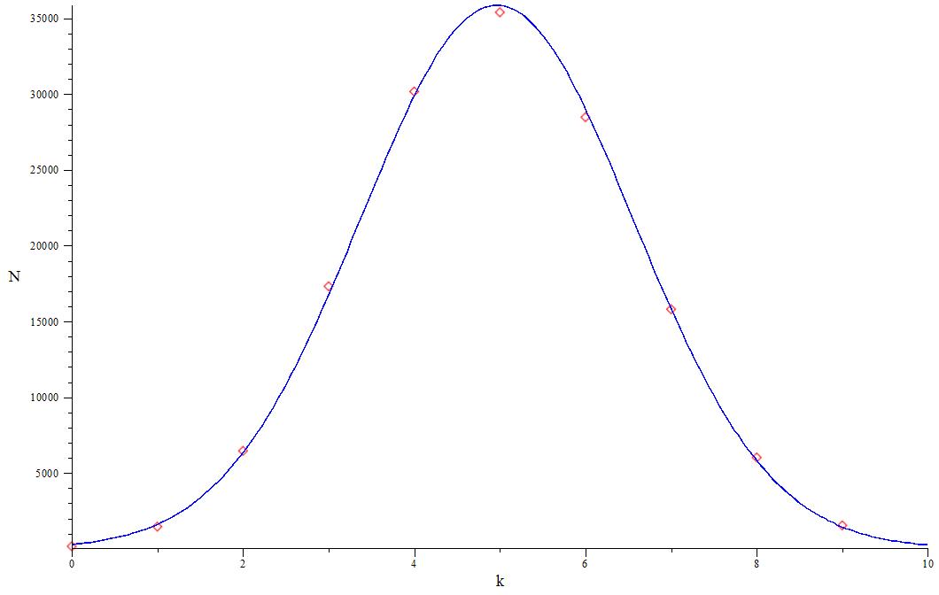
Figure 3: Red dots are $\hat{N}^{c=1}_{[2],-11,k}$ numbers, blue curve is a Gaussian distribution with parameters $\mu=4.96$ $\sigma=1.59$ $I=1.43\cdot 10^{5}$

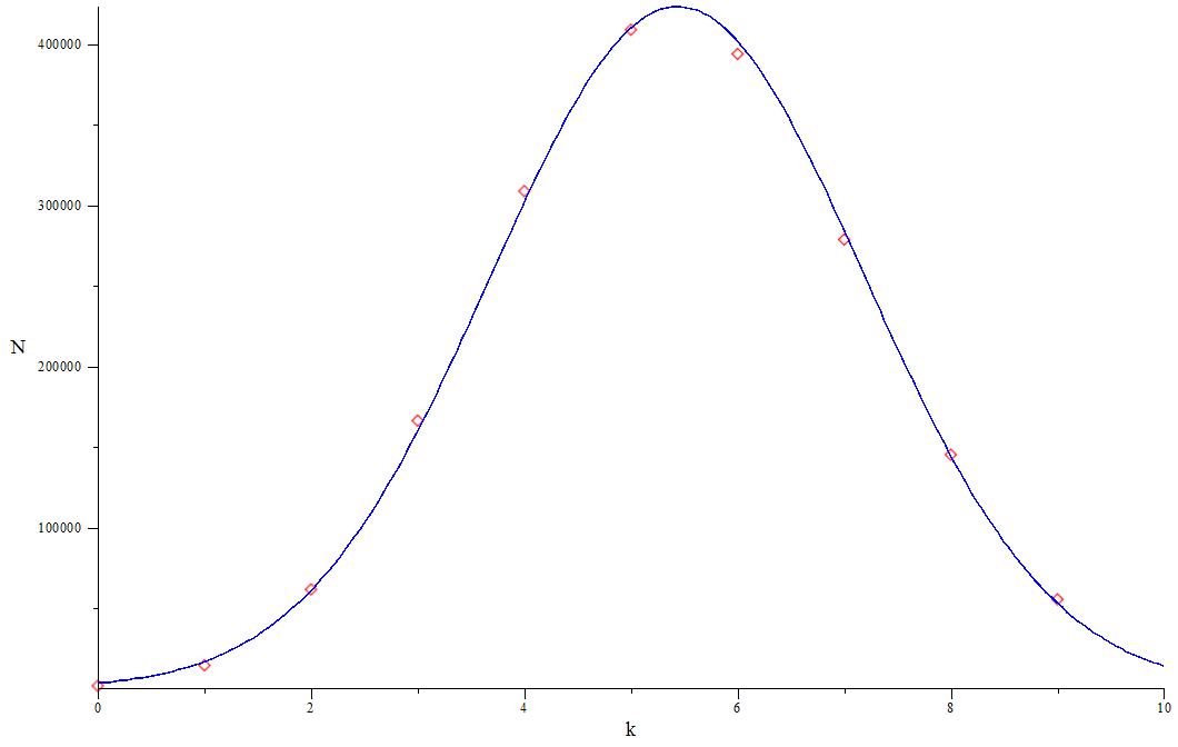
Figure 4: Red dots are $\hat{N}^{c=1}_{[1,1],-7,k}$ numbers, blue curve is a Gaussian distribution with parameters $\mu=5.44$ $\sigma=1.75$ $I=1.85\ 10^{6}$

6 Conclusion

In this paper, we reported a positive result of new tests of the LMOV integrality conjectures, made possible by a recent progress in evaluation of the colored knot polynomials and first corollary of the performed calculations: the Gaussian distribution of the LMOV invariants. The progress is a cumulative effect of merging of the different research directions:

• reformulation of the RT formalism in the spaces of intertwining operators [31]-[35] with developments of the highest weight technique [19, 21] and the eigenvalue conjecture [33, 1] to evaluate the inclusive and exclusive Racah matrices [21]-[23],

• representing the knot polynomials for all arborescent knots through the exclusive Racah matrices $S$ and $\bar{S}$ [17],

• developing the family technique [77, 18, 20] in order to adequately classify knots, at least, for calculational purposes,

• applying Vogel’s universality [85] to handle the adjoint representations and their descendants; important here is that deviations from the universality at the group theory level are not seen in knot polynomial calculus [74, 1].

The work in all these directions is hard, but interesting and important (see also a new development in another direction of an integrality conjecture for superpolynomials, [86]). The integrality tests are a non-trivial application of its results, and provide an additional stimulus for new advances.

References

- [1] A. Mironov and A. Morozov, Phys. Lett. B755 (2016) 47-57, arXiv:1511.09077
- [2] R.Gopakumar and C.Vafa, Adv.Theor.Math.Phys. 3 (1999) 1415-1443, hep-th/9811131; hep-th/9812127
- [3] H. Ooguri and C. Vafa, Nucl.Phys. B577 (2000) 419-438, arXiv:hep-th/9912123
-
[4]
S.-S. Chern and J. Simons,
Ann.Math. 99 (1974) 48-69
E. Witten, Comm.Math.Phys. 121 (1989) 351-399 -
[5]
J.W. Alexander, Trans.Amer.Math.Soc. 30 (2) (1928) 275-306
V.F.R. Jones, Invent.Math. 72 (1983) 1 Bull.AMS 12 (1985) 103 Ann.Math. 126 (1987) 335
L. Kauffman, Topology 26 (1987) 395
P. Freyd, D. Yetter, J. Hoste, W.B.R. Lickorish, K. Millet, A. Ocneanu, Bull. AMS. 12 (1985) 239
J.H. Przytycki and K.P. Traczyk, Kobe J. Math. 4 (1987) 115-139 - [6] J.H. Conway, Algebraic Properties, In: John Leech (ed.), Computational Problems in Abstract Algebra, Proc. Conf. Oxford, 1967, Pergamon Press, Oxford-New York, 329-358, 1970
- [7] J.M.F. Labastida and M. Mariño, Commun.Math.Phys. 217 (2001) 423-449, hep-th/0004196
- [8] J.M.F. Labastida, M. Mariño and C. Vafa, JHEP 0011 (2000) 007, hep-th/0010102
- [9] J.M.F. Labastida and M. Mariño, math/0104180
- [10] M. Mariño and C. Vafa, hep-th/0108064
-
[11]
S. Garoufalidis, P. Kucharski and P. Sułkowski, Commun.Math.Phys. 346 (2016) 75-113, arXiv:1504.06327
P. Kucharski and P. Sułkowski, JHEP 11 (2016) 120, arXiv:1608.06600
Wei Luo and Shengmao Zhu, arXiv:1611.06506 -
[12]
P. Ramadevi, T.R. Govindarajan and R.K. Kaul,
Mod.Phys.Lett. A9 (1994) 3205-3218, hep-th/9401095
S. Nawata, P. Ramadevi and Zodinmawia, J.Knot Theory and Its Ramifications 22 (2013) 13, arXiv:1302.5144
Zodinmawia’s PhD thesis, 2014 - [13] D. Galakhov, D. Melnikov, A. Mironov, A. Morozov and A. Sleptsov, Phys.Lett. B743 (2015) 71-74, arXiv:1412.2616
- [14] A. Mironov, A. Morozov and A. Sleptsov, JHEP 07 (2015) 069, arXiv:1412.8432
- [15] D. Galakhov, D. Melnikov, A. Mironov and A. Morozov, Nucl.Phys. B899 (2015) 194-228, arXiv:1502.02621
- [16] S. Nawata, P. Ramadevi and Vivek Kumar Singh, arXiv:1504.00364
- [17] A. Mironov, A. Morozov, An. Morozov, P. Ramadevi, and Vivek Kumar Singh, JHEP 1507 (2015) 109, arXiv:1504.00371
- [18] A.Mironov and A.Morozov, Nucl.Phys. B899 (2015) 395-413, arXiv:1506.00339
- [19] A. Mironov, A. Morozov, An. Morozov and A. Sleptsov, J. Mod. Phys. A30 (2015) 1550169, arXiv:1508.02870
- [20] A. Mironov, A. Morozov, An. Morozov, P. Ramadevi, Vivek Kumar Singh and A. Sleptsov, arXiv:1601.04199
- [21] A. Mironov, A. Morozov, An. Morozov and A. Sleptsov, arXiv:1605.02313
- [22] A. Mironov, A. Morozov, An. Morozov and A. Sleptsov, arXiv:1605.03098
- [23] A. Mironov, A. Morozov, An. Morozov and A. Sleptsov, Physics Letters B760 (2016) 45-58, arXiv:1605.04881
- [24] http://knotebook.org
-
[25]
M. Khovanov, Duke Math.J. 101 (2000) no.3, 359426, math/9908171;
Experimental Math. 12 (2003) no.3, 365374, math/0201306;
J.Knot theory and its Ramifications 14 (2005) no.1, 111-130, math/0302060;
Algebr. Geom. Topol. 4 (2004) 1045-1081, math/0304375;
Int.J.Math. 18 (2007) no.8, 869885, math/0510265; math/0605339; arXiv:1008.5084
D. Bar-Natan, Algebraic and Geometric Topology 2 (2002) 337-370, math/0201043; Geom.Topol. 9 (2005) 1443-1499, math/0410495; J.Knot Theory Ramifications 16 (2007) no.3, 243255, math/0606318
M. Khovanov and L. Rozansky, Fund. Math. 199 (2008), no. 1, 191, math/0401268; Geom.Topol. 12 (2008), no. 3, 13871425, math/0505056; math/0701333
N. Carqueville and D. Murfet, arXiv:1108.1081
V. Dolotin and A. Morozov, JHEP 1301 (2013) 065, arXiv:1208.4994; J. Phys. 411 012013, arXiv:1209.5109; Nucl.Phys. B878 (2014) 12-81, arXiv:1308.5759
A. Anokhina and A. Morozov, JHEP 07 (2014) 063, arXiv:1403.8087
S. Nawata and A. Oblomkov, arXiv:1510.01795
D. Galakhov and G. Moore, arXiv:1607.04222
S. Gukov, Du Pei, P. Putrov and C. Vafa, arXiv:1701.06567 -
[26]
N.Yu. Reshetikhin and V.G. Turaev, Comm. Math. Phys. 127 (1990) 1-26
E. Guadagnini, M. Martellini and M. Mintchev, Clausthal 1989, Procs.307-317; Phys.Lett. B235 (1990) 275
V.G. Turaev and O.Y. Viro, Topology 31, 865 (1992)
A. Morozov and A. Smirnov, Nucl.Phys. B835 (2010) 284-313, arXiv:1001.2003
A. Smirnov, Proc. of International School of Subnuclar Phys. Erice, Italy, 2009, arXiv:hep-th/0910.5011 -
[27]
R.K. Kaul, T.R. Govindarajan, Nucl.Phys. B380 (1992)
293-336, hep-th/9111063; ibid. B393 (1993) 392-412
P. Ramadevi, T.R. Govindarajan and R.K. Kaul, Nucl.Phys. B402 (1993) 548-566, hep-th/9212110; Nucl.Phys. B422 (1994) 291-306, hep-th/9312215; Mod.Phys.Lett. A10 (1995) 1635-1658, hep-th/9412084 - [28] P. Ramadevi and T. Sarkar, Nucl.Phys. B600 (2001) 487-511, hep-th/0009188
- [29] P. Borhade, P. Ramadevi and T. Sarkar, Nucl.Phys. B678 (2004) 656-681, hep-th/0306283
- [30] P. Ramadevi and Zodinmawia, arXiv:1107.3918; arXiv:1209.1346
-
[31]
A. Mironov, A. Morozov and An. Morozov, in: Strings, Gauge Fields, and the Geometry Behind: The Legacy of Maximilian Kreuzer, edited by A.Rebhan, L.Katzarkov, J.Knapp, R.Rashkov, E.Scheidegger (World Scietific Publishins Co.Pte.Ltd. 2013) pp.101-118, arXiv:1112.5754; JHEP 03 (2012) 034, arXiv:1112.2654
A. Anokhina, A. Mironov, A. Morozov and An. Morozov, Nucl.Phys. B868 (2013) 271-313, arXiv:1207.0279
A. Anokhina, arXiv:1412.8444 - [32] H. Itoyama, A. Mironov, A. Morozov and An. Morozov, IJMP A27 (2012) 1250099, arXiv:1204.4785
- [33] H. Itoyama, A. Mironov, A. Morozov and An. Morozov, IJMP A28 (2013) 1340009, arXiv:1209.6304
- [34] A. Anokhina, A. Mironov, A. Morozov and An. Morozov, Adv.High Energy Physics, 2013 (2013) 931830, arXiv:1304.1486
- [35] A. Anokhina and An. Morozov, Theor.Math.Phys. 178 (2014) 1-58, arXiv:1307.2216
- [36] E. Witten, J. Differential Geom. 17 (1982), 661-692
- [37] A. Kapustin and E. Witten, Commun. Numb. Th. Phys. 1 (2007) 1-236, hep-th/0604151
- [38] E. Witten, in R. Kirby, V. Krushkal, and Z. Wang, eds., Proceedings Of The FreedmanFest (Mathematical Sciences Publishers, 2012) 291-308, arXiv:1108.3103; arXiv:1401.6996; arXiv:1603.03854
- [39] D.E. Littlewood, The theory of group characters and matrix representations of groups, Oxford, 1958
- [40] P. Dunin-Barkowski, A. Mironov, A. Morozov, A. Sleptsov and A. Smirnov, JHEP 03 (2013) 021, arXiv:1106.4305
- [41] A. Mironov, A. Morozov and Sh. Shakirov, J. Phys. A: Math. Theor. 45 (2012) 355202, arXiv:1203.0667
- [42] J.J. Duistermaat and G. Heckman, Inv. Math. 69 (1982) 259-269, ibid. 72 (1983) 153-158
-
[43]
M. Blau, E. Keski-Vakkuri and A.J. Niemi, Phys. Lett. B246 (1990) 92-98
A.Yu. Morozov, A.J. Niemi and K. Palo, Phys. Lett. B271 (1991) 365-371
A. Hietamaki, A.Yu. Morozov, A.J. Niemi and K. Palo, Phys. Lett. B263 (1991) 417-424 -
[44]
A. S. Schwarz and O. Zaboronsky, Commun.Math.Phys. 183 (1997) 463 476, hep-th/9511112
C. Beasley and E. Witten, J.Diff.Geom. 70 (2005) 183 323, hep-th/0503126 - [45] J. Kallen, JHEP 1108 (2011) 008, arXiv:1104.5353
- [46] V. Pestun, Commun.Math.Phys. 313 (2012) 71-129, arXiv:0712.2824
-
[47]
A. Alexandrov, A. Mironov and A. Morozov,
Physica D235 (2007) 126-167, hep-th/0608228; JHEP 12 (2009) 053, arXiv:0906.3305
B. Eynard and N. Orantin, Commun. Number Theory Phys. 1 (2007) 347-452, math-ph/0702045
N. Orantin, arXiv:0808.0635 -
[48]
M. Tierz, Mod. Phys. Lett. A19 (2004) 1365-1378, hep-th/0212128
A.Brini, B.Eynard and M.Mariño, Annales Henri Poincaré. Vol. 13. No. 8. SP Birkhäuser Verlag Basel, 2012, arXiv:1105.2012 -
[49]
A.Alexandrov, A.Mironov, A.Morozov and An.Morozov,
JETP Letters 100 (2014) 271-278 (Pis’ma v ZhETF 100 (2014) 297-304), arXiv:1407.3754
A. Alexandrov and D. Melnikov, arXiv:1411.5698 - [50] R.Dijkgraaf, H.Fuji and M.Manabe, Nucl.Phys. B849 (2011) 166-211, arXiv:1010.4542
-
[51]
A. Mironov, A. Morozov and A.Sleptsov, Theor.Math.Phys. 177 (2013) 179-221, arXiv:1303.1015;
The European Physical Journal, C73 (2013) 2492, arXiv:1304.7499
A. Mironov, A. Morozov, A. Sleptsov and A. Smirnov, Nucl.Phys. B889 (2014) 757-777, arXiv:1310.7622
A. Sleptsov, Int.J.Mod.Phys. A29 (2014) 1430063 - [52] A. Mironov, A. Morozov and S. Natanzon, Theor.Math.Phys. 166 (2011) 1-22, arXiv:0904.4227; Journal of Geometry and Physics 62 (2012) 148-155, arXiv:1012.0433
-
[53]
A. Alexandrov, A. Mironov, A. Morozov and S. Natanzon, J. Phys. A: Math. Theor. 45 (2012) 045209, arXiv:1103.4100;
JHEP 11 (2014) 080, arXiv:1405.1395
A. Mironov, A. Morozov and S. Natanzon, JHEP 11 (2011) 097, arXiv:1108.0885 - [54] W.Fulton, Young tableaux: with applications to representation theory and geometry, London Mathematical Society, 1997
- [55] R. Dijkgraaf, Progress in Math. 129 (1995), 149-163, Brikhäuser
- [56] A. Okounkov, Math.Res.Lett. 7 (2000) 447-453
- [57] A. Mironov, A. Morozov, S. Shakirov and A. Smirnov, Nucl. Phys. B855 (2012) 128, arXiv:1105.0948
- [58] http://knotebook.org.s3-website-us-west-2.amazonaws.com/knotebook/HOMFLY/colored.htm
- [59] http://knotebook.org.s3-website-us-west-2.amazonaws.com/knotebook/HOMFLY/kauffman.htm
- [60] http://knotebook.org.s3-website-us-west-2.amazonaws.com/knotebook/HOMFLY/universal.htm
- [61] K. Liu and P. Peng, J. Diff. Geom. 85 (2010), no. 3 479-525, arXiv:0704.1526; Math.Res.Lett. 17 (2010) 493-506, arXiv:1012.2635
- [62] M. Marino, Commun.Math.Phys. 298 (2010) 613 643, arXiv:0904.1088
- [63] S. Stevan, Annales Henri Poincare 11 (2010) 1201-1224, arXiv:1003.2861
- [64] C. Paul, P. Borhade and P. Ramadevi, arXiv:1003.5282; Nucl.Phys. B841 (2010) 448-462, arXiv:1008.3453
- [65] S. Nawata, P. Ramadevi and Zodinmawia, JHEP 1401 (2014) 126, arXiv:1310.2240
-
[66]
A. Caudron, Classification des noeuds et des enlacements, Publ. Math. Orsay
82-4, University of Paris XI, Orsay, 1982
F. Bonahon and L. C. Siebenmann, http://www-bcf.usc.edu/fbonahon/Research/Preprints/BonSieb.pdf, New geometric splittings of classical knots and the classification and symmetries of arborescent knots, 2010 - [67] D. Bar-Natan and S. Morrison, http://katlas.org
- [68] M. Aganagic and C. Vafa, hep-th/0012041
- [69] S. Sinha and C. Vafa, hep-th/0012136
- [70] V. Bouchard, B. Florea and M. Mariño, JHEP 0412 (2004) 035, hep-th/0405083; JHEP 0502 (2005) 002, hep-th/0411227
- [71] P. Borhade and P. Ramadevi, Nucl.Phys. B727 (2005) 471-498, hep-th/0505008
-
[72]
L. Rudolph, Math. Proc. Cambridge Philos. Soc. 107 (1990) 319 327
H.R. Morton, Algebr. Geom. Topol. 7 (2007) 327-338
H.R. Morton and N.D.A. Ryder, arXiv:math.GT/0902.1339 - [73] K. Koike, Adv. Math. 74 (1989) 57
- [74] A. Mironov, R. Mkrtchyan, A. Morozov, JHEP 02 (2016) 78, arXiv:1510.05884
- [75] N.M. Dunfield, S. Gukov and J. Rasmussen, Experimental Math. 15 (2006) 129-159, math/0505662
- [76] H. Itoyama, A. Mironov, A. Morozov and An. Morozov, JHEP 2012 (2012) 131, arXiv:1203.5978
-
[77]
A. Mironov, A. Morozov and An. Morozov, AIP Conf. Proc. 1562 (2013) 123, arXiv:1306.3197
S. Arthamonov, A. Mironov, A. Morozov and An. Morozov, JHEP 04 (2014) 156, arXiv:1309.7984 - [78] S. Arthamonov, A. Mironov and A. Morozov, Theor.Math.Phys. 179 (2014) 509-542, arXiv:1306.5682
- [79] S. Gukov, S. Nawata, I. Saberi, M. Stosic and P. Sulkowski, arXiv:1512.07883
- [80] Ya. Kononov and A. Morozov, Pisma v ZhETF 101 (2015) 931934, arXiv:1504.07146
- [81] A. Morozov, arXiv:1605.09728; arXiv:1606.06015
- [82] I. Tuba and H. Wenzl, math/9912013
- [83] S. Nawata, P. Ramadevi and Zodinmawia, Lett.Math.Phys. 103 (2013) 1389-1398, arXiv:1302.5143
- [84] J. Gu and H. Jockers, arXiv:1407.5643
- [85] P. Vogel, The universal Lie algebra, preprint (1999), see at http://webusers.imj-prg.fr/pierre.vogel/
- [86] M. Kameyama and S. Nawata, Refined large N duality with torus knots, to appear