Visualizing Efimov Correlations in the Bose Polaron

Abstract

The Bose polaron is a quasi-particle of an impurity dressed by surrounding bosons. In few-body physics, it is known that two identical bosons and a third distinguishable particle can form a sequence of Efimov bound states in the vicinity of inter-species scattering resonance. On the other hand, in the Bose polaron system with an impurity atom embedded in many bosons, no signature of Efimov physics has been reported in the existing spectroscopy measurements up to date. In this work, we propose that a large mass imbalance between a light impurity and heavy bosons can help produce visible signatures of Efimov physics in such a spectroscopy measurement. Using the diagrammatic approach in the Virial expansion to include three-body effects from pair-wise interactions, we determine the impurity self-energy and its spectral function. Taking ⁶Li-¹³³Cs system as a concrete example, we find two visible Efimov branches in the polaron spectrum, as well as their hybridizations with the attractive polaron branch. We also discuss the general scenarios for observing the signature of Efimov physics in polaron systems. This work paves the way for experimentally exploring intriguing few-body correlations in a many-body system in the near future.

Top-down and bottom-up are two major approaches to studying correlations in a quantum many-body system. The cold atom system has intrinsic advantage for the bottom-up approach since it is a dilute system and the few-body problems therein are well understood. In this approach, one would like to understand how many-body physics is built up from few-body correlations. In cold atom system, one of the most intriguing three-body correlations lies in Efimov physics, which is characterized by an infinite number of trimer states nearby a two-body resonance and following a universal scaling law Efimov ; Braaten . Efimov physics has been observed in a number of cold atoms experiments, while all of them are at the few-body levelEfimov_Exp0 ; Efimov_Exp1 ; Efimov_Exp1bu ; Efimov_Exp3 ; Efimov_Exp4 ; Efimov_Exp5 ; Efimov_Exp9 ; Efimov_Exp10 ; Efimov_Exp6 ; Efimov_Exp7 ; Efimov_Exp8 ; Efimov_Exp11 ; rf_1 ; rf_2 ; scaling_1 ; scaling_2 ; scaling_3 . The manifestation of Efimov physics in the many-body system has yet to be observed.

In this context, a convenient and non-trivial testbed is the highly-polarized ultracold gases, which consist of minority impurity atoms interacting with the majority of fermionic or bosonic atoms, respectively called the Fermi or the Bose polarons. Lots of theoretical efforts have been paid to study the Fermi polaron Chevy ; Lobo ; Combescot1 ; Combescot2 ; Prokofev ; Punk ; Enss ; Cui ; Troyer ; Bruun ; Parish ; Zhou ; Zinner1 ; Nishida ; Cui1 ; Cui2 and the Bose polaron Pitaevskii ; Timmermans ; Blume ; Jaksch ; Huang ; Schmidt ; LiWeiran ; Wouters ; Demler1 ; Demler2 ; Devreese ; Zinner2 ; Levinsen1 ; Levinsen2 ; Giorgini ; Shchadilova . Nearby a Feshbach resonance, a Fermi polaron displays an attractive branch Chevy ; Lobo ; Combescot1 ; Combescot2 ; Prokofev ; Punk ; Enss and a repulsive branch Cui ; Troyer ; Bruun , which directly manifests two-body correlations in this system. In the past few years, the Fermi polaron has been studied by a number of experiments Zwierlein ; Salomon ; Grimm ; Kohl ; Grimm2016 ; Roati , while the Bose polaron has only recently been exploredAarhus ; JILA ; Lamb . Most of these experiments are the injection radio-frequency spectroscopy measurements, with which both the repulsive and the attractive branches have been observed Grimm ; Kohl ; Grimm2016 ; Roati ; Aarhus ; JILA .

From the bottom-up point of view, a difference between the Bose polarons Aarhus ; JILA ; Lamb and the Fermi polarons Zwierlein ; Salomon ; Grimm ; Kohl ; Grimm2016 ; Roati already exists in the three-body system consisting of two majority atoms and a third distinguishable particle (usually denoted by ”BB+X”), where the Bose systems exhibit the Efimov effect while the Fermi systems do not, because Efimov physics is facilitated by the Bose statistics Efimov ; Braaten . So far, the spectroscopy measurements of the Bose polarons by the Aarhus Aarhus and JILA JILA groups have not detected such extra Efimov correlation. Despite a few theoretical investigations of the three-body correlations in the Fermi polaron Parish ; Zhou ; Zinner1 ; Nishida ; Cui1 ; Cui2 and the Bose polaron Levinsen1 ; Levinsen2 ; Giorgini , it is still not clear under what circumstances, the spectroscopy measurement can reveal this difference. Nevertheless, the theoretical treatment of the Bose polaron problem is quite challenging, as it should work for the strong coupling regime and take into account the three-body effects in a non-perturbative way. So far the theoretical tools for this purpose have been quite limited, including the variational approach with truncated number of boson excitations Levinsen2 and the diffusion Monte Carlo methodGiorgini . It is thus imperative to develop an alternative method with controllable approximation for the problem in order to further guide the experiments.

Before going to details, let us summarize that, with the explicit calculation presented in this work, we can understand the challenge of observing the signature of Efimov physics in the Bose polarons as follows: Comparing the size of Efimov trimers in vacuum $l_{t}$ and the mean distance of background many-body system $d$, if $l_{t}\gg d$, which usually occurs for shallow Efimov trimers near resonance (see Fig.1(a)), their effect can be easily washed out by two-body correlations and is very difficult to resolve in experiments; if $l_{t}\ll d$, which occurs for deep Efimov trimers, their effect is also difficult to resolve in the injection spectroscopy of polarons due to the little wave function overlap with the initial scattering state. Therefore the most favorable situation is $l_{t}\sim d$.

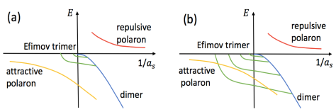
Figure 1: (Color Online). Schematics of two scenarios of Efimov trimers in vacuum (green lines) with respect to attractive and repulsive branches of a Bose polaron (orange and red lines). (a) supports shallow Efimov trimers with large scaling factor, while (b) supports reasonably deep trimers with small scaling factor. In (b), the trimer levels can be close or level-crossing with the attractive polaron branch. The signature of Efimov physics will be visible in the spectral function of the Bose polaron in (b) but is hardly visible in (a).

In this work, we propose to utilize the large mass imbalance between the impurity and the bosons to facilitate the observation of Efimov correlations in the Bose polarons. Our main results can be illustrated in Fig.1 by comparing two scenarios classified by the mass ratio $\eta=m_{\text{b}}/m_{\text{i}}$, where $m_{\text{b}}\ (m_{\text{i}})$ is the boson (impurity) mass. For the Efimov trimers of heteronuclear atomic systems, when $\eta\ll 1$, the scaling factor is largeBraaten , and the trimers are generally quite shallow and appear only close to the resonanceGreene , see Fig.1(a). Thus the Efimov correlation is hardly visible in the Bose polarons considering $l_{t}\gg d$. The Aarhus experiment with two different hyperfine states of ³⁹K ($\eta=1$)Aarhus and the JILA experiment with ⁴⁰K impurity in ⁸⁷Rb ($\eta=87/40$)JILA both belong to this scenario.

When $\eta\gg 1$, the scaling factor is small and the Efimov spectrum is dense Braaten ; meanwhile, the lowest Efimov trimer can appear far from resonance and can be quite deeply bound at resonanceGreene . Thus, some of the trimers can have the chance to fall into the $l_{t}\sim d$ regime which makes Efimov signatures visible in the Bose polarons, and the visibility can be further enhanced if these trimers are very close or level-crossing with the attractive polaron branch, as shown in Fig. 1(b). Fortunately, taking the experimentally well studied ⁶Li-¹³³Cs system as an example, our calculation shows two visible Efimov branches in the spectral response of an ⁶Li impurity immersed in ¹³³Cs bosons, and their hybridizations with the attractive polaron branch causing the spectral broadening and enhanced Efimov signals. The unique response properties revealed in this work suggest that the highly mass-imbalanced polaron systems can serve as an ideal platform for detecting intriguing few-body correlations in a many-body environment.

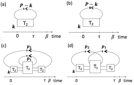
Figure 2: Feynman diagrams for the impurity self energy $\Sigma^{(1)}$ (a) and $\Sigma^{(2)}$(b-d). $T_{2}$ and $T_{3}$ are respectively the two-body and atom-dimer scattering matrixes; $\tilde{T}_{3}$ is $T_{3}$ excluding the first Born term in Eq.6 (i.e., excluding reducible diagrams). The boson propagator line with $n$ vertical dashes denotes the $n$-th order contribution $G^{(0,n)}$ in Eq. 2.

Formalism. Here we adopt the diagrammatic approach in the framework of the Virial expansion Kaplan ; Leyronas1 ; Leyronas2 ; Hofmann1 ; Ngampruetikorn ; Hofmann2 . The advantage of this method is that it is accurate at high temperature, and can systematically incorporate all the two-body and three-body contributions which allow us to extract the Efimov effect in a controllable way. The Hamiltonian of this $1+N$ system is written as

$$\mathcal{H}=\frac{{\bf p}_{i}^{2}}{2m_{\text{i}}}+\sum\limits_{j=1}^{N}\frac{{\bf p}_{j}^{2}}{2m_{\text{b}}}+\sum\limits_{j=1}^{N}V({\bf r}_{i}-{\bf r}_{j}),$$ (1)

where ${\bf r}_{i}$ and ${\bf p}_{i}$ label the position and momentum of the impurity atom, while ${\bf r}_{j}$ and ${\bf p}_{j}$ ($j=1,\dots,N$) label the position and momentum of $N$ majority bosons. The impurity-boson interaction $V({\bf r})$ is described by an $s$-wave scattering length $a_{\text{s}}$, which can be tuned across resonance. Note that here we have neglected the background boson-boson interaction for simplicity. The starting point is to expand the free boson propagator in powers of the fugacity $z_{b}=e^{\beta\mu_{b}}$ ($\mu_{\text{b}}$ is the boson chemical potential, $\beta=1/(k_{\text{B}}T)$):

$$G^{(0)}(\mathbf{p},\tau)=e^{\mu\tau}\sum_{n\geq 0}G^{(0,n)}(\mathbf{p},\tau)z_{b}^{n},$$ (2)

where $G^{(0,n)}(\mathbf{p},\tau)$ is $-\Theta(\tau)e^{-\tau\epsilon_{\mathbf{p}}}$ for $n=0$ and $-e^{-n\beta\epsilon_{\mathbf{p}}}e^{-\epsilon_{\mathbf{p}}\tau}$ for $n\geqslant 1$; $\tau\in(0,\beta]$ is the imaginary time; $\epsilon_{\mathbf{p}}={\bf p}^{2}/(2m_{b})$; $n_{b}(x)=1/(e^{\beta x}-1)$ is the Bose distribution function. With Eq. 2, all physical quantities can be expanded in powers of $z_{b}$.

In Fig. 2 we plot the Feynman diagrams for the impurity self-energy $\Sigma({\bf k},\tau)$, which contain all the two-body and three-body diagrams that contribute to the second and the third Virial coefficient ($b_{2}$ and $b_{3}$) in the Virial expansion. Fig. 2(a) leads to the lowest order of $\Sigma$ in $z_{b}$, denoted by

$$\Sigma^{(1)}=z_{b}\int\frac{d^{3}\mathbf{P}}{(2\pi)^{3}}e^{-\beta\epsilon_{\mathbf{P-k}}}T_{2}\left(\omega+i\delta+\epsilon_{\mathbf{P-k}}-\frac{P^{2}}{2(m_{i}+m_{b})}\right);$$ (3)

Fig. 2(b-d) leads to the second order contribution as:

$$\Sigma^{(2)}=z_{b}^{2}\left\{\int\frac{d^{3}\mathbf{P}}{(2\pi)^{3}}e^{-2\beta\epsilon_{\mathbf{P-k}}}T_{2}\left(\omega+i\delta+\epsilon_{\mathbf{P-k}}-\frac{P^{2}}{2(m_{i}+m_{b})}\right)\right.$$

$$+\int\frac{d^{3}\mathbf{p_{1}}}{(2\pi)^{3}}\int\frac{d^{3}\mathbf{p_{2}}}{(2\pi)^{3}}e^{-\beta(\epsilon_{\mathbf{p_{1}}}+\epsilon_{\mathbf{p_{2}}})}T_{2}^{2}\left(\omega+i\delta+\Delta-\frac{{p_{1}^{\prime}}^{2}}{2m_{AD}}\right)T_{3}(\mathbf{p^{\prime}_{1}},\mathbf{p^{\prime}_{1}},\omega+i\delta+\Delta)$$

$$+\left.\int\frac{d^{3}\mathbf{p_{1}}}{(2\pi)^{3}}\int\frac{d^{3}\mathbf{p_{2}}}{(2\pi)^{3}}e^{-\beta(\epsilon_{\mathbf{p_{1}}}+\epsilon_{\mathbf{p_{2}}})}T_{2}\left(\omega+i\delta+\Delta-\frac{{p^{\prime}_{1}}^{2}}{2m_{AD}}\right)\tilde{T}_{3}(\mathbf{p^{\prime}_{1}},\mathbf{p^{\prime}_{2}},\omega+i\delta+\Delta)T_{2}\left(\omega+i\delta+\Delta-\frac{{p^{\prime}_{2}}^{2}}{2m_{AD}}\right)\right\}.$$ (4)

Here $\Delta=\epsilon_{\mathbf{p_{1}}}+\epsilon_{\mathbf{p_{2}}}-P_{t}^{2}/(2M)$, with $\mathbf{P_{t}}=\mathbf{k}+\mathbf{p_{1}}+\mathbf{p_{2}}$ and $M=2m_{b}+m_{i}$ respectively the total momentum and the total mass of three-body system; $\mathbf{p^{\prime}_{1,2}}=\mathbf{p_{1,2}}-m_{b}\mathbf{P_{t}}/M$ and $m_{AD}=m_{b}(m_{b}+m_{i})/M$ are respectively the relative momenta and the reduced mass for atom-dimer scattering. $T_{2}(E)$ is the two-body scattering matrix with scattering energy $E$:

$$T_{2}(E)=\frac{2\pi}{m_{r}}\frac{1}{a_{s}^{-1}-\sqrt{-2m_{r}E}},$$ (5)

where $m_{r}=\frac{m_{b}m_{i}}{m_{b}+m_{i}}$ is the reduced mass. $T_{3}(\mathbf{p_{1}},\mathbf{p_{2}},E)$ is the atom-dimer scattering matrix at energy $E$, with $\mathbf{p_{1}},\mathbf{p_{2}}$ respectively the relative momenta of the incoming and outgoing atom-dimer states in the center-of-mass frame, and

$$T_{3}(\mathbf{p_{1}},\mathbf{p_{2}},E)=\frac{1}{E-\epsilon_{\mathbf{p}_{1}}-\epsilon_{\mathbf{p}_{2}}-(\mathbf{p}_{1}+\mathbf{p}_{2})^{2}/(2m_{i})}$$

$$+\int\frac{d^{3}\mathbf{q}}{(2\pi)^{3}}\frac{T_{2}(E-\frac{q^{2}}{2m_{AD}})}{E-\epsilon_{\mathbf{p}_{1}}-\epsilon_{\mathbf{q}}-\frac{(\mathbf{p}_{1}+\mathbf{q})^{2}}{2m_{i}}}T_{3}(\mathbf{q},\mathbf{p_{2}},E).$$ (6)

To this end we have obtained the impurity self-energy, $\Sigma=\Sigma^{(1)}+\Sigma^{(2)}$, up to the order of $z_{b}^{2}$. The spectral function can be computed from the propagator of the impurity, $G_{i}({\mathbf{k}},\omega)=(\omega+i\delta-k^{2}/(2m_{i})-\Sigma({\mathbf{k}},\omega+i\delta))^{-1}$, as

$$A({\mathbf{k}},\omega)=-\frac{1}{\pi}{\rm Im}\Big{(}G_{i}({\mathbf{k}},\omega)\Big{)}.$$ (7)

As a benchmark for our calculation, we have obtained the trimer energy $E_{T}^{(n)}$ at resonance from the pole of $T_{3}$ and determined the scattering length $a_{-}^{(n)}$ for the appearance of the $n$-th trimer state in $a_{s}<0$ side. We have verified that both $a_{-}^{(n)}$ and $E_{T}^{(n)}$ well follow the universal scaling law for large $n$, i.e., $a_{-}^{(n)}/a_{-}^{(n+1)}=\lambda$, $E_{T}^{(n)}/E_{T}^{(n+1)}=\lambda^{2}$, with $\lambda$ the scaling factorEfimov ; Braaten . We have also obtained $b_{3}$ with the same diagrams for $\Sigma^{(2)}$, and the result well reproduces the known analytical behaviors in both unitary and deep molecular regimes Hofmann2 .

Results. In Table 1 we compare $\eta$, $\lambda$, $\alpha^{(n)}\equiv 1/(k_{F}a_{-}^{(n)})$ and $\epsilon^{(n)}\equiv E_{T}^{(n)}/E_{F}$ for three different impurity-boson(i-b) systems, where $k_{F}=(6\pi^{2}n_{b})^{1/3},\ E_{F}=k_{F}^{2}/(2m_{b})$ and we take a typical density $n_{b}=2\times 10^{14}$cm^-3 for all boson systems. The three-body cutoff is chosen such that the obtained $a_{-}^{(1)}$ for different systems match the values in Refs.Aarhus ; Greene ; scaling_2 . Since the size of the trimer at resonance follows $l_{t}/d\propto\epsilon^{-1/2}$, the large (or small) $\epsilon$ corresponds to $l_{t}\ll d$ (or $l_{t}\gg d$). From the table, we can see that the first two systems, ³⁹K-³⁹K(i-b) and ⁴⁰K-⁸⁷Rb(i-b), both belong to case (a) in Fig. 1, where the trimers appear only sufficiently close to resonance ($|\alpha^{(n)}|\ll 1$) with their sizes $l_{t}\gg d$; while the third system, ⁶Li-¹³³Cs(i-b), belongs to case (b), where the first and the second trimers appear with $|\alpha^{(n)}|\sim 1$, and as varying $1/a_{s}$, these trimers can have sizes $l_{t}\sim d$.

impurity-boson	$\eta$	$\lambda$	$\alpha^{(1)}$	$\alpha^{(2)}$	$\alpha^{(3)}$	$\epsilon^{(1)}$	$\epsilon^{(2)}$	$\epsilon^{(3)}$
39K-39K Aarhus	1	1986	$-2.76\times 10^{-3}$	$-1.39\times 10^{-6}$	$-6.99\times 10^{-10}$	$1.51\times 10^{-4}$	$3.84\times 10^{-11}$	$9.73\times 10^{-18}$
40K-87Rb JILA	$2.2$	123	$-2.76\times 10^{-2}$	$-2.23\times 10^{-4}$	$-1.82\times 10^{-6}$	$1.40\times 10^{-2}$	$9.32\times 10^{-7}$	$6.19\times 10^{-11}$
6Li-133Cs scaling_2 ; scaling_3	$22.2$	$4.87$	$-2.56$	$-0.40$	$-7.87\times 10^{-2}$	185.9	6.09	0.25

Table 1: Mass ratio ($\eta\equiv m_{b}/m_{i}$), Efimov scaling factor from zero-range theory ($\lambda$), the interaction parameter for the appearance of the $n$-th Efimov trimers ($\alpha^{(n)}\equiv 1/(k_{F}a_{-}^{(n)})$), and the $n$-th trimer energy at resonance ($\epsilon^{(n)}\equiv E_{T}^{(n)}/E_{F}$) for three systems with different impurity-boson(i-b) combinations. The values of $a_{-}^{(1)}$ are from Refs.Aarhus ; Greene ; scaling_2 . For Li-Cs system, the relatively large derivation of the scaling factor for the two lowest trimer states from $\lambda$ is due to the very deep lowest trimer (with $E_{T}^{(1)}$ of the order of the cutoff energy), in which the finite range effect becomes non-negligible.

Below we present the spectral results for ³⁹K-³⁹K(i-b) system (Fig. 3) and ⁶Li-¹³³Cs(i-b) system (Fig. 4) as the representatives of two cases in Fig. 1. Since the injection spectroscopy used in the experiments Grimm ; Kohl ; Grimm2016 ; Roati ; Aarhus ; JILA can be described by $A(\mathbf{k}=0,\omega)$, taking $z_{b}=0.1$ for both systems (giving the thermal wavelength $\lambda_{T}=0.47d$), we show the contour plots of $A(0,\omega)$ in terms of $1/(k_{F}a_{s})$ and $\omega/E_{F}$ in Fig. 3(a) and 4(a), and slices of $A(0,\omega)$ in Fig. 3(b) and 4(b) for several typical values of $-1/(k_{F}a_{s})$ across resonance.

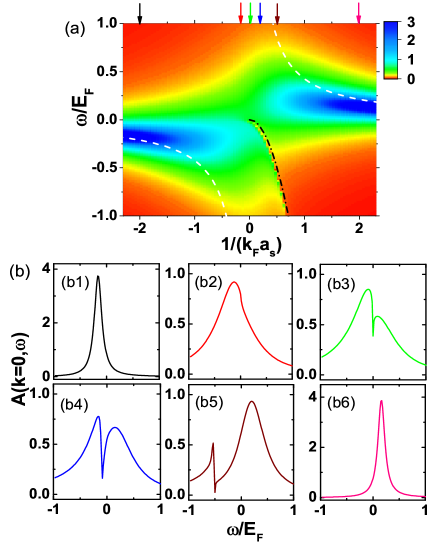
Figure 3: (Color online). Spectral function $A(\mathbf{k}=0,\omega)$ (in unit of $1/E_{F}$) for ³⁹K-³⁹K(i-b) system. (a) shows the contour plot of $A(\mathbf{k}=0,\omega)$ in term of $1/(k_{F}a_{s})$ and $\omega/E_{F}$. For comparison, we show the two-body binding energy (black dashed-dot) and the mean-field energies of attractive and repulsive branches (white dashed). (b) shows slices of $A(\mathbf{k}=0,\omega)$ for $1/(k_{F}a_{s})=-2,-0.2,0,0.2,0.5,2$ (from (b1) to (b6)), as labeled by the arrows in (a) with according colors. Here $z_{b}=0.1$.

In Fig. 3, the spectrum shows only attractive and repulsive polaron branches without any signature of Efimov physics. It shows that, at least in the temperature regime we are considering, the Efimov signature is not visible if $l_{t}\gg d$. As increasing $1/(k_{F}a_{s})$, the spectrum starts from a well-defined quasi-particle peak centered at negative $\omega$ (attractive polaron, Fig. 3(b1)), which gradually becomes broader (Fig. 3(b2)) to exhibit a two-peak structure near resonance (Fig. 3(b3-b5), and finally evolves to a single peak centered at positive $\omega$ (repulsive polaron, Fig. 3(b6)). All these features are consistent with current experimental observations Aarhus ; JILA .

Contrarily, in Fig. 4, besides the attractive and repulsive branches, there are two visible Efimov branches, which are associated with the first two Efimov trimers in vacuum emerging at $a_{-}^{(1,2)}<0$ (dotted lines in Fig. 4(a)). Interestingly, these Efimov branches can be very close or even level-crossing with the attractive branch of polarons, and the inter-branch hybridization leads to a much broadened spectrum near $a_{s}\sim a_{-}^{(1)}$ as well as an enhanced signal of the second Efimov branch near resonancefootnote .

Figure 4: (Color online). Same plot of $A(\mathbf{k}=0,\omega)$ as in Fig. 3 but for ⁶Li-¹³³Cs (i-b) system. From (b1) to (b6), $1/(k_{F}a_{s})=-3,-2.5,-2,-0.2,0,2$. The additional dotted lines in (a) show the energies of the first and the second Efimov trimers from three-body calculations. The gray arrows in (b2,b4,b5) mark the spectral peaks of the Efimov branches.

In this case, starting from a single attractive polaron branch (Fig. 4(b1)), with the increase of $1/(k_{F}a_{s})$, one can see the first Efimov branch appears around $a_{s}\sim a_{-}^{(1)}$ with a narrow peak near zero frequency (marked by the arrow in Fig. 4(b2)) and it hybridizes with the attractive polaron branch. This Efimov branch quickly merges into the attractive polaron branch away from their (avoided) level-crossing (Fig. 4(b3)). The second Efimov branch shows up as a nearby resonance (arrow in Fig. 4(b4)), and its signal can become more pronounced when its level moves closer to the attractive branch (Fig. 4(b5)). Finally it becomes a single branch at positive frequency (repulsive polaron, Fig. 4(b6)).

Note that the Efimov branches shown in Fig. 4 are only visible after including the three-body contributions ($\Sigma^{(2)}$). In contrast, we have checked that the inclusion of $\Sigma^{(2)}$ in Fig. 3 does not make qualitative change to the spectrum. This confirms the distinct roles of three-body effect played in the two systems, as illustrated in Fig. 1.

Another notable difference between Fig. 3 and Fig. 4 is that in the latter, the attractive and repulsive branches have much narrower relative spectral width, defined by the ratio of the absolute width to the mean location of the spectral peak. Near resonance, these branches are well separated and disconnected, unlike those in Fig. 3. This suggests that for given $\lambda_{T}/d$, the Bose polaron quasi-particle is more well-defined for larger mass ratio $\eta$.

Discussion and Outlook. In this work, we have revealed the signature of Efimov physics in the spectral response of the Bose polarons with large mass imbalance. The setting here is different from previous ones exploring the energetics of the Bose polarons with relatively small mass imbalanceLevinsen2 ; Giorgini . Nevertheless, the phenomenon of avoided level crossing shown in Fig.4 is physically in accordance with atom-trimer continuity in the ground state of the Bose polarons as studied in Ref.Levinsen2 .

Our results (assuming no interaction between bosons) can be directly probed in ⁶Li-¹³³Cs atomic system near $B_{0}=889$G Feshbach resonancenew_expt1 ; new_expt2 , where the boson-boson scattering length ($a_{bb}$) is small and the Efimov scenario is not modified by finite $a_{bb}$ (except for the ground state trimernew_expt1 ). Moreover, the diagrammatic approach we used in this work can be generalized to interacting boson systems, with the boson-boson interaction contributing to another scattering channel. Our method can also be systematically improved to include $n$-body correlations ($n>3$) in a controllable matter, for instance, the effect of four-body bound states consisting of one ⁶Li and three ¹³³Cs atoms Blume2 , which may result in additional signals near the location of their appearances.

In principle, our results can also be applied to the Fermi polarons. However, for the reduced three-body problem from Fermi polarons, the Efimov states appear only when the mass ratio exceeds $13.6$Petrov . Just above the critical mass ratio, the Efimov trimers are shallow and the scaling factor is large, so the system falls into the scenario (a) discussed here. Thus, in order to observe the signature of Efimov physics in Fermi polarons, one needs the mass ratio far exceeding $13.6$.

Acknowledgements. We thank Ran Qi, Cheng Chin, Jesper Levinsen, Ren Zhang, Pengfei Zhang and Zhigang Wu for helpful discussions, and the Supercomputer Center in Guangzhou for computational support. This work is supported by the National Natural Science Foundation of China (No. 11626436, 11374177, 11421092, 11534014, 11325418), the National Key Research and Development Program of China (No. 2016YFA0300603, 2016YFA0301600), and Tsinghua University Initiative Scientific Research Program.

References

- (1) V. Efimov, Yad. Fiz. 12, 1080 (1970); Sov. J. Nucl. Phys. 12, 589 (1971).
- (2) E. Braaten and H.-W. Hammer, Phys. Rep. 428, 259 (2006).
- (3) T. Kraemer, M. Mark, P. Waldburger, J. G. Danzl, C. Chin, B. Engeser, A. D. Lange, K. Pilch, A. Jaakkola, H.-C. Nägerl and R. Grimm, Nature 440, 315 (2006).
- (4) T. B. Ottenstein, T. Lompe, M. Kohnen, A. N. Wenz, and S. Jochim, Phys. Rev. Lett. 101, 203202 (2008).
- (5) J. R. Williams, E. L. Hazlett, J. H. Huckans, R. W. Stites, Y. Zhang, and K. M. O’Hara, Phys. Rev. Lett. 103, 130404 (2009).
- (6) M. Zaccanti, B. Deissler, C. D’Errico, M. Fattori, M. Jona-Lasinio, S. Müller, G. Roati, M. Inguscio and G. Modugno, Nat. Phys. 5, 586 (2009).
- (7) N. Gross, Z. Shotan, S. Kokkelmans and L. Khaykovich, Phys. Rev. Lett. 103, 163202 (2009).
- (8) S. E. Plooack, D. Dries and R. G. Hulet, Science 326, 1683 (2009).
- (9) S. Knoop, F. Ferlaino, M. Mark, M. Berninger, H. Schöbel, H.-C. Nägerl, and R. Grimm, Nat. Phys. 5, 227 (2009).
- (10) S. Nakajima, M. Horikoshi, T. Mukaiyama, P. Naidon and M. Ueda, Phys. Rev. Lett. 105, 023201 (2010).
- (11) T. Lompe, T. B. Ottenstein, F. Serwane, K. Viering, A. N. Wenz, G. Zürn, and S. Jochim, Phys. Rev. Lett. 105,103201 (2010)
- (12) M. Berninger, A. Zenesini, B. Huang, W. Harm, H.-C. Nägerl, F. Ferlaino, R. Grimm, P. S. Julienne and J. M. Hutson, Phys. Rev. Lett. 107, 120401 (2011).
- (13) R. J. Wild, P. Makotyn, J. M. Pino, E. A. Cornell and D. S. Jin, Phys. Rev. Lett. 108, 145305 (2012).
- (14) R. S. Bloom, M.-G. Hu, T. D. Cumby, and D. S. Jin, Phys. Rev. Lett. 111, 105301 (2013).
- (15) T. Lompe, T.B. Ottenstein, F. Serwane, A.N. Wenz, G. Zürn, S. Jochim, Science 330, 940 (2010).
- (16) S. Nakajima, M. Horikoshi, T. Mukaiyama, P. Naidon, and M. Ueda, Phys. Rev. Lett. 106, 143201 (2011).
- (17) B. Huang, L. A. Sidorenkov, R. Grimm and J. M. Hutson, Phys. Rev. Lett. 112, 190401 (2014).
- (18) S.-K. Tung, K. Jimenez-Garcia, J. Johansen, C. V. Parker, and C. Chin, Phys. Rev. Lett. 113, 240402 (2014).
- (19) R. Pires, J. Ulmanis, S. Hafner, M. Repp, A. Arias, E. D. Kuhnle, and M. Weidemuller, Phys. Rev. Lett. 112, 250404 (2014).
- (20) F. Chevy, Phys. Rev. A 74, 063628 (2006).
- (21) C. Lobo, A. Recati, S. Giorgini, and S. Stringari, Phys. Rev. Lett. 97, 200403 (2006).
- (22) R. Combescot, A. Recati, C. Lobo, and F. Chevy, Phys. Rev. Lett. 98, 180402 (2007).
- (23) R. Combescot and S. Giraud, Phys. Rev. Lett. 101, 050404 (2008).
- (24) N. V. Prokofev and B. V. Svistunov, Phys. Rev. B 77, 125101 (2008).
- (25) M. Punk, P. T. Dumitrescu, and W. Zwerger, Phys. Rev. A 80, 053605 (2009).
- (26) X. Cui and H. Zhai, Phys. Rev. A 81, 041602(R) (2010).
- (27) S. Pilati, G. Bertaina, S. Giorgini, and M. Troyer, Phys. Rev. Lett. 105, 030405 (2010).
- (28) P. Massignan and G. M. Bruun, Eur. Phys. J. D 65, 83 (2011).
- (29) R. Schmidt and T. Enss, Phys. Rev. A 83, 063620 (2011).
- (30) C. J. M. Mathy, M. M. Parish, and D. A. Huse, Phys. Rev. Lett. 106, 166404 (2011).
- (31) D. J. MacNeill and F. Zhou, Phys. Rev. Lett. 106, 145301 (2011).
- (32) N. G. Nygaard and N. T. Zinner, New J. Phys. 16, 023026 (2014).
- (33) Y. Nishida, Phys. Rev. Lett. 114, 115302 (2015).
- (34) W. Yi and X. Cui, Phys. Rev. A 92, 013620 (2015).
- (35) X. Qiu, X. Cui and W. Yi, Phys. Rev. A 94, 051604 (2016).
- (36) G. E. Astrakharchik and L. P. Pitaevskii, Phys. Rev. A 70, 013608 (2004).
- (37) F. M. Cucchietti and E. Timmermans, Phys. Rev. Lett. 96, 210401 (2006).
- (38) R. M. Kalas and D. Blume, Phys. Rev. A 73, 043608 (2006).
- (39) M. Bruderer, W. Bao, and D. Jaksch, Europhysics Letters 82, 30004 (2008).
- (40) B.-B. Huang and S.-L. Wan, Chinese Physics Letters 26, 080302 (2009).
- (41) S. P. Rath and R. Schmidt, Phys. Rev. A 88, 053632 (2013).
- (42) W. Li and S. Das Sarma, Phys. Rev. A 90, 013618 (2014).
- (43) W. Casteels and M. Wouters, Phys. Rev. A 90, 043602 (2014).
- (44) A. Shashi, F. Grusdt, D. A. Abanin, and E. Demler, Phys. Rev. A 89, 053617 (2014).
- (45) F. Grusdt, Y. E. Shchadilova, A. N. Rubtsov, and E. Demler, Sci. Rep. 5, 12124 (2015).
- (46) J. Vlietinck, W. Casteels, K. V. Houcke, J. Tempere, J. Ryckebusch, and J. T. Devreese, New Journal of Physics 17, 033023 (2015).
- (47) A. G. Volosniev, H.-W. Hammer, and N. T. Zinner, Phys. Rev. A 92, 023623 (2015).
- (48) R. S. Christensen, J. Levinsen, and G. M. Bruun, Phys. Rev. Lett. 115, 160401 (2015).
- (49) J. Levinsen, M. M. Parish and G. M. Bruun, Phys. Rev. Lett. 115, 125302 (2015).
- (50) L. A. Pena Ardila and S. Giorgini, Phys. Rev. A 92, 033612 (2015); ibid, Phys. Rev. A 94, 063640 (2016).
- (51) Y. E. Shchadilova, R. Schmidt, F. Grusdt and E. Demler, Phys. Rev. Lett. 117, 113002 (2016).
- (52) A. Schirotzek, C.-H. Wu, A. Sommer, and M. W. Zwierlein, Phys. Rev. Lett. 102, 230402 (2009).
- (53) S. Nascimbéne, N. Navon, K. J. Jiang, L. Tarruell, M. Teichmann, J. McKeever, F. Chevy, and C. Salomon, Phys. Rev. Lett. 103, 170402 (2009).
- (54) C. Kohstall, M. Zaccanti, M. Jag, A. Trenkwalder, P. Massignan, G. M. Bruun, F. Schreck, R. Grimm, Nature 485, 615 (2012).
- (55) M. Koschorreck, D. Pertot, E. Vogt, B. Frölich, M. Feld, M. Köhl, Nature 485, 619 (2012).
- (56) M. Cetina, M. Jag, R. S. Lous, I. Fritsche, J. T. M. Walraven, R. Grimm, J. Levinsen, M. M. Parish, R. Schmidt, M. Knap, E. Demler, Science 354, 96 (2016).
- (57) F. Scazza, G. Valtolina, P. Massignan, A. Recati, A. Amico, A. Burchianti, C. Fort, M. Inguscio, M. Zaccanti, G. Roati, arxiv:1609.09817.
- (58) N. B. Jrgensen, L. Wacker, K. T. Skalmstang, M. M. Parish, J. Levinsen, R. S. Christensen, G. M. Bruun, J. J. Arlt, Phys. Rev. Lett. 117, 055302 (2016).
- (59) M.-G. Hu, M. J. Van de Graaff, D. Kedar, J. P. Corson, E. A. Cornell, D. S. Jin, Phys. Rev. Lett. 117, 055301 (2016).
- (60) T. Rentrop, A. Trautmann, F. A. Olivares, F. Jendrzejewski, A. Komnik and M. K. Oberthaler, Phys. Rev. X 6, 041041 (2016).
- (61) Y. Wang, J. Wang, J. P. D’Incao, and C. H. Greene, Phys. Rev. Lett. 109, 243201 (2012).
- (62) D. B. Kaplan and S. Sun, Phys. Rev. Lett. 107, 030601 (2011).
- (63) X. Leyronas, Phys. Rev. A 84, 053633 (2011).
- (64) V. Ngampruetikorn, J. Levinsen, and M. M. Parish, Phys. Rev. Lett. 111, 265301 (2013).
- (65) M. Barth and J. Hofmann, Phys. Rev. A 89, 013614 (2014).
- (66) M. Sun and X. Leyronas, Phys. Rev. A 92, 053611 (2015).
- (67) M. Barth and J. Hofmann, Phys. Rev. A 92, 062716 (2015).
- (68) In Fig. 4 there exists a very small parameter regime nearby zero energy where becomes negative after including , and we attribute this to the convergency problem of the Virial expansion and the absence of higher-order contributions of beyond the level.
- (69) D. S. Petrov, Phys. Rev. A 67, 010703(R) (2003).
- (70) J. Ulmanis, S. Hafner, R. Pires, E. D. Kuhnle, Y. Wang, C. H. Greene, and M. Weidemueller, Phys. Rev. Lett. 117, 153201 (2016).
- (71) J. Johansen, B. J. DeSalvo, K. Patel, and C. Chin, arxiv:1612.05169.
- (72) D. Blume and Y. Yan, Phys. Rev. Lett. 113, 213201 (2014).