Minimally-corrected partial atomic charges for non-covalent electrostatic interactions

Abstract

We develop a new scheme for determining molecular partial atomic charges (PACs) with external electrostatic potential (ESP) closely mimicking that of the molecule. The PACs are the “minimal corrections” to a reference-set of PACs necessary for reproducing exactly the tensor components of the Cartesian zero- first- and second- molecular electrostatic multipoles. We evaluate the quality of ESP reproduction when “minimally correcting” (MC) Mulliken, Hirshfeld or iterated-Hirshfeld reference PACs. In all these cases the MC-PACs significantly improve the ESP while preserving the reference PACs’ invariance under the molecular symmetry operations. When iterative-Hirshfeld PACs are used as reference the MC-PACs yield ESPs of comparable quality to those of the ChElPG charge fitting method.

1 Introduction

Partial atomic charges (PACs), i.e. point charges placed on the nuclei position of a molecule are often used in large-scale molecular mechanics calculations to replace the detailed quantum mechanical charge distributions. ^{1, 2, 3, 4, 5, 6, 7} The model is extremely useful since by using them the long-range electrostatic forces acting between molecules can be expressed as a sum of pairwise interactions, enabling a fast computation, important especially as molecules jiggle around and rotate quite a lot during the course of the simulation. The question of just how to determine PACs for this purpose is critical. We argue that the most important constraint is the exact reproduction of the low-order electrostatic moments (ESM), the monopole $Q=e\int\rho\left(\boldsymbol{r}\right)d\boldsymbol{r}$, which is the total charge of the system, the dipole $\mu_{i}=e\int\rho\left(\boldsymbol{r}\right)r_{i}d\boldsymbol{r}$ ($i=x,y,z$) and the quadrupole moment $\Theta_{ij}=e\int\rho\left(\boldsymbol{r}\right)\left(3r_{i}r_{j}-\delta_{ij}r^{2}\right)d\boldsymbol{r}$, where $e\rho\left(\boldsymbol{r}\right)$ is the charge distribution within the molecule. These moments are of critical importance as they determine the far-field potential produced by the molecule , as evident from the monopole expnasion:

$$4\pi\epsilon_{0}\varphi\left(\boldsymbol{r}\right) \equiv e\int\rho\left(\boldsymbol{r}^{\prime}\right)\left|\boldsymbol{r}-\boldsymbol{r}^{\prime}\right|^{-1}d\boldsymbol{r}^{\prime}$$ (1)

$$=\frac{Q}{r}+\frac{\mu_{i}r_{i}}{r^{3}}+\frac{1}{2}\frac{r_{i}\Theta_{ij}r_{j}}{r^{5}}+....$$ (2)

These low-order ESMs also control the electrostatic interaction energy $W_{es}$ between the molecule (and through it the forces) with a weakly non-constant potential $\varphi^{other}\left(\boldsymbol{r}\right)$ resulting from the other molecules or distant charged sources⁸:

$$W_{es}=Q\varphi^{other}+\mu_{i}\varphi_{i}^{other}+\frac{1}{6}\Theta_{ij}\varphi_{ij}^{other}+\dots$$ (3)

where $\varphi_{i}^{other}=\frac{\partial\varphi^{other}}{\partial r_{i}}$ and $\varphi_{ij}^{other}=\frac{\partial^{2}\varphi^{other}}{\partial r_{i}\partial r_{j}}$ (estimated at a central point within the molecule) etc. This pivotal dual role of ESMs is what drives the requirement that the charge distribution of the PACs reproduce exactly low-lying molecular ESMs (MOL-ESMs). This point was discussed at length in ref. ⁹ where the importance of adherence to the ESMs was demonstrated. An efficient elegant method for achieving this in as many as possible moments has been developed ¹⁰ although inapplicable for large molecule charges due to numerical instabilities.¹¹

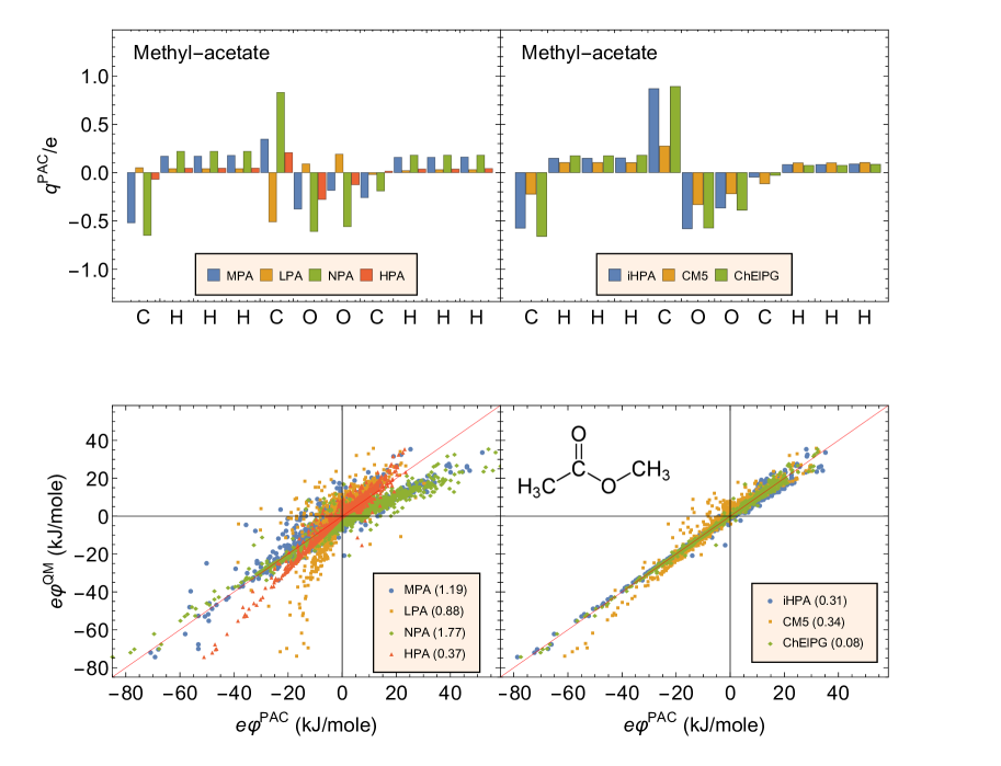
Figure 1: The PACs (top panels) and the ESP correlation (bottom panels) for the methyl-acetate molecule, using standard population analysis methods (left panels) and other PAC methods (right panels). The mean absolute relative deviation (MARD) of Eq. 5 appears in parenthesis near each PAC method. Each point in the ESP correlation plot describes a pair of potentials $\left[\varphi^{PAC}\left(\boldsymbol{r}\right),\varphi^{QM}\left(\boldsymbol{r}\right)\right]$, the abscissa is the PAC potential (Eq. (4)) and the ordinate the quantum potential (Eq. (1)) where $\boldsymbol{r}$ is taken from a subset of grid points of spacing $\Delta x=0.3\mathring{A}$ around the molecule (see description of the grid in Section (3)).

Another source of PACs are the quantum mechanical population analysis (PA) techniques, such as the Mulliken (MPA),¹², Loewdin (LPA),¹³, Hirshfeld (HPA)¹⁴, and natural population (NPA)¹⁵ analyses. These PAs reflect not only the charge distribution but also aspects of the quantum mechanical wave function. In Fig. 1 (top left) we show as bar-plot the PACs produced by these methods applied to the methyl acetate molecule. It is seen that the different methods produce sometimes significantly different sets of PACs, even PAC signs are not preserved! For example, the LPA assigns positive charges to oxygen atoms, which seems awkward given their high electronegativity. Furthermore, standard PAs do not reproduce the MOL-ESPs closely, as shown in the ESP correlation plot of Fig. 1 (bottom left), where several PAC-ESPs,

$$\varphi^{PAC}\left(\boldsymbol{r}\right)=\frac{e}{4\pi\epsilon_{0}}\sum_{a}\frac{q_{a}}{\left|\boldsymbol{r}-\boldsymbol{R}_{a}\right|},$$ (4)

are plotted vs. the MOL-ESP $\varphi\left(\boldsymbol{r}\right)$ calculated from the QM density (Eq. 1) at a grid point $\boldsymbol{r}$. The thin red line in the plot corresponds to the perfectly correlated condition $\varphi^{PAC}=\varphi^{QM}$. In order to quantify the quality of $\varphi^{PAC}\left(\boldsymbol{r}\right)$ we define the mean absolute relative deviation (MARD) from $\varphi\left(\boldsymbol{r}\right)$ as

$$MARD\left(\varphi^{PAC},\varphi\right)=\left\langle\left|\frac{\varphi^{PAC}\left(\boldsymbol{r}\right)-\varphi\left(\boldsymbol{r}\right)}{\varphi\left(\boldsymbol{r}\right)}\right|\right\rangle,$$ (5)

where an average is taken over all grid-points $\boldsymbol{r}$ for which: 1) $\boldsymbol{r}$ is “outside of the molecule”, i.e. its distance from any nucleus $a$ is larger than the atomic van-der-Waals radius $R_{a}^{vdW}$ ¹⁶) and 2) $\boldsymbol{r}$ is not too far from the molecule, so that its potential $\left|\varphi\left(\boldsymbol{r}\right)\right|$ is not smaller than the threshold value of $e\varphi_{thresh}=0.3eV$. PACs obtained by “standard” PAs have large MARDs: ranging from 0.37 for HPA up to a whopping 1.76 for NPA. On the right panel of the figure we show data concerning the same molecule, but using the iterated-Hirshfeld method (iHPA),^{17, 18, 19} the CM5 method ²⁰, which is a parameterized database correction to HPA charges, and the ChElPG method²¹, which selects PACs that reconstruct the ab initio ESP on a set of grid points as close as possible. The latter approach is taken here as representative of a class of methods routinely used for PACs determination. Other members of this method class are the “charge from ESPs” (ChElP)²², the Merz-Kollman^{23, 16, 24}, the charge-restraint ESPs (RESP)^{25, 26}, atomic multipoles ESPs²⁷, in combination with molecular multipoles²⁸ (related to the method proposed here), the dynamical RESP (D-RESP)²⁹ and Hu-Yang fitting³⁰.The iHPA, CM5 and ChElPG methods yield much improved description of the ESP with MARD going from 0.3 for iHPA and CM5 down to 0.08 for ChElPG. Despite the close ESP fit, ChElPG produces PACs that are usually not invariant under transformations preserving the point symmetry of the molecule or under rotations or translations of the nuclei with respect to the real space grid used to perform the fit. Furthermore, in larger molecules the PACs of atoms distant from the molecular surface can become unwieldy large. Both of these issues are discussed in the literature^{31, 30}This instability is likely linked to the fact that the number of parameters derivable from the ESP in a statistically significant way is considerably less than the number of atoms.³² Therefore, iHPA and CM5 are often considered preferred approaches for PACs, although as seen in the figure, both methods leave ample room for improvement. Note that the iHPA charges for this molecule are close to the ChElPG PACs.

Here, we study a new idea: take PACs which are as close as possible to a reference set, for example the MPA, HPA or iHPA PACs, but insist that they reproduce exactly the components of the lowest ESM tensors (dipole and quadrupole) characterizing the molecular charge distribution. We formulate a straightforward method to determine such “minimally-corrected PACs” (section 2) and then benchmark the results using a subset of molecules taken from the database of ref. ²⁰ (section 3). Final conclusions are summarized in section 4. All MPA, HPA and iHPA PACs, as well as the associated MOL-ESPs and MOL-ESMs were computed using developer versions of Q-Chem 4.3 and 4.4 ³³ at the M06-L DFT level ³⁴ and using the MG3 semi-diffuse (MG3S) basis set ³⁵. This functional/basis set combination was used for developing of the CM5 approach. The CM5, NPA and LPA results were taken from ref. 20.

2 Method

Consider a molecule having $A$ nuclei at given Cartesian positions $\boldsymbol{R}^{a}=\left(R_{x}^{a},\,R_{y}^{a},\,R_{z}^{a}\right)$ ($a=1,\dots,A$), for which a QM calculation has determined the charge density $\rho\left(\boldsymbol{r}\right)$ of the molecule and from it, low order moments the charge $Q$, the dipole $\mu_{i}$ and the symmetric traceless quadrupole moment tensor $\Theta_{ij}$. Note that below, we use the notation $\Theta_{i}^{D}\equiv\Theta_{ii}$ for the diagonal elements of $\Theta$ and $\Theta_{i}^{OD}\equiv\Theta_{jk}$ where $i=x,y,z$ and $ijk$ is a cyclic permutation of $xyz$. For any set of PACs $\boldsymbol{q}=\left(q_{1},\dots,q_{A}\right)$ we define the PAC-ESMs as: the monopole (total charge) $Q^{PAC}\equiv e\sum_{a}q_{a}$, the dipole $\mu_{i}^{PAC}\equiv e\sum_{a}q_{a}R_{i}^{a}$ and the quadrupole $\Theta_{ij}^{PAC}\equiv e\sum_{a}q_{a}\left(3R_{i}^{a}R_{j}^{a}-\delta_{ij}\left(R^{a}\right)^{2}\right)$, ($i,j=x,y,z$) . Given a set of reference PACs $\boldsymbol{q}^{ref}$ we seek to determine a “minimally-corrected” set of PACs $\boldsymbol{q}^{mc}=\boldsymbol{q}^{ref}+\Delta\boldsymbol{q}$ such that that the size of the correction $\left\|\Delta\boldsymbol{q}\right\|^{2}=\Delta\boldsymbol{q}\cdot\Delta\boldsymbol{q}$ is minimal but the multipoles are equal to the QM determined multipoles, i.e. the following constraints are satisfied:

$$c =Q-Q^{PAC}=0,$$

$$c_{i} =\mu_{i}-\mu_{i}^{PAC}=0,$$ (6)

$$c_{ij} =\Theta_{ij}-\Theta_{ij}^{PAC}=0.$$

Note that the number of constraints (denoted $C$) in Eq. (6) is $9$ and not $13$ since the electric quadrupole tensor is symmetric and traceless. Point symmetries can reduce this number of constraints further. If, for example, both positive and negative charge densities are symmetric against the reflection through a plane (the x-y plane, for example) then there are 3 constraint less (one from the z component of the dipole and and 2 from XZ and YZ components of the quadrupole, which are zero by symmetry). Only when the number of atoms $A$ in the molecule is greater than the number of constraints $C$ can we hope to reproduce the constraints exactly. We therefore demand that $A>9$ and use the $A-C$ additional “degrees of freedom” to minimize the deviance $\Delta\boldsymbol{q}$. When $2\leq A\leq 9$ we avoid the quadrupole moment constraint and use only the dipole moment constraint.

We are led to consider the Lagrangian

$$L_{mcDQ} =\frac{1}{2}\sum_{a}\left(q_{a}^{mc}-q_{a}^{ref}\right)^{2}-\lambda c-\lambda_{i}c_{i}$$ (7)

$$-\sum_{xy,yz,zx}\lambda_{ij}^{OD}c_{ij}-\sum_{x,y,z}\lambda_{ii}^{D}c_{ii}$$

as a function of the $A$ $q^{\prime}s$ and the ten Lagrange multipliers: one $\lambda,$ three $\lambda_{i}$’s , three diagonal $\lambda_{ii}^{D}$ and three off-diagonal$\lambda_{jk}^{OD}$ where $i=x,y,z$ and $ijk$ is a cyclic permutation of $xyz$. Taking derivatives with respect to these variables and equating to zero leads to the following set of $\left(10+A\right)$ linear equations in $\left(10+A\right)$ unknowns, given here in block-matrix/vector form:

$$S \left(\begin{array}[]{c}q_{1}^{mc}\\ \vdots\\ q_{A}^{mc}\\ \lambda_{1\times 1}\\ \lambda_{3\times 1}\\ \lambda_{3\times 1}^{D}\\ \lambda_{3\times 1}^{OD}\end{array}\right)=\left(\begin{array}[]{c}q_{1}^{ref}\\ \vdots\\ q_{A}^{ref}\\ Q_{1\times 1}\\ \mu_{3\times 1}\\ \Theta_{3\times 1}^{D}\\ \Theta_{3\times 1}^{OD}\end{array}\right).$$ (22)

The $\left(A+10\right)\times\left(A+10\right)$ matrix $S$ is of the following form:

$$S=\left(\begin{array}[]{ccccccccccccc}\text{\textSFi}&\cdots&\text{\textSFiii}&-1&\text{\textSFi}&&\text{\textSFiii}&\text{\textSFi}&&\text{\textSFiii}&\text{\textSFi}&&\text{\textSFiii}\\ \vdots&I_{A\times A}&\vdots&\vdots&\vdots&-D_{A\times 3}&\vdots&\vdots&-T_{A\times 3}^{D}&\vdots&\vdots&-T_{A\times 3}^{OD}&\vdots\\ \text{\textSFii}&\cdots&\text{\textSFiv}&-1&\text{\textSFii}&&\text{\textSFiv}&\text{\textSFii}&&\text{\textSFiv}&\text{\textSFii}&&\text{\textSFiv}\\ 1&\cdots&1&0&0&0&0&0&0&0&0&0&0\\ \text{\textSFi}&\cdots&\text{\textSFiii}&0&0&0&0&0&0&0&0&0&0\\ &D_{3\times A}&&0&0&0&0&0&0&0&0&0&0\\ \text{\textSFii}&\cdots&\text{\textSFiv}&0&0&0&0&0&0&0&0&0&0\\ \text{\textSFi}&\cdots&\text{\textSFiii}&0&0&0&0&0&0&0&0&0&0\\ &T_{3\times A}^{D}&&0&0&0&0&0&0&0&0&0&0\\ \text{\textSFii}&\cdots&\text{\textSFiv}&0&0&0&0&0&0&0&0&0&0\\ \text{\textSFi}&\cdots&\text{\textSFiii}&0&0&0&0&0&0&0&0&0&0\\ &T_{3\times A}^{OD}&&0&0&0&0&0&0&0&0&0&0\\ \text{\textSFii}&\cdots&\text{\textSFiv}&0&0&0&0&0&0&0&0&0&0\end{array}\right)$$ (23)

and depends only on the location of the atomic nuclei. The matrix is composed of blocks: the $I_{A\times A}$ block is a $A\times A$ unit matrix, $D_{A\times 3}$, $T_{A\times 3}^{D}$ and $T_{A\times 3}^{OD}$ are matrices of dimension $A\times 3$ ($3$ columns each of length $A$) of matrix elements: $D_{ai}=eR_{i}^{a}$ and $T_{ai}^{D}=e\left(3R_{i}^{a}R_{i}^{a}-\|R^{a}\|^{2}\right)$ for $a=1,\dots,A$ and $i=x,y,z$ and and $T_{ai}^{OD}=3eR_{j}^{a}R_{k}^{a}$ (where the ordered set $i,j,k$ is a cyclic permutation of $x,y,z$). The $D_{3\times A}$, $T_{3\times A}^{D}$, and $T_{3\times A}^{OD}$ blocks are respectively the transposed matrices. The $A+10$ column-vector on the left-hand-side of Eq. 22 includes the unknowns, the $A$ partial charges $q_{a}^{mc}$ and the $\lambda^{\prime}s$, the ten Lagrange multipliers for the ten constraints. The $10+A$ column-vector on the right-hand-side has $A$ values of the reference charges $q_{a}^{ref}$, followed by the total charge on the molecule $Q$, then the three values of the QM dipole moment $\mu_{i}$ followed by the three values of the diagonal elements of the given QM quadrupole tensor $\Theta_{i}^{D}=\Theta_{ii}$ and finally the QM values of the three off-diagonal elements $\Theta_{i}^{OD}=\Theta_{jk}$ where $i=x,y,z$ and $ijk$ is a cyclic permutation of $xyz$). A similar equation holds for the mcD method, where the six last rows are erased from $S$ and from the column vectors and the six right columns are erased from $S$ as well. This leaves us with a $\left(A+4\right)\times\left(A+4\right)$ system of equations.

The structural matrix $S$ may become singular or rank deficient. One trivial source for singularity the use of 3 diagonal constraints while their sum is composed to be zero. The use of the singular-value-decomposition pseudo-inverse ³⁶ for solving Eq. 22 helps to bypass such a singularity. A more delicate source of singularities may arise from symmetry. For example, when the molecule is perfectly planar (or has a plane of symmetry) in the x-y plane then the row corresponding to the dipole in the z direction $D_{az}=eR_{z}^{a}$ must be identically zero and the matrix $S$ will be rank deficient. In this case the $T_{ai}^{OD}$ with $i=x$and $y$ must also be zero). In these cases the SVD pseudoinverse will automatically eliminate constraints that cannot be met due to this kind of symmetry. But for near-symmetrical configurations, instabilities may exist. In cases such as these we can still spot problems by examining the values of the Lagrange multipliers $\lambda,$$\lambda_{i}$ and $\lambda_{ij}$in the solution vector of Eq. 22. The Lagrange multiplier is equal to the derivative of the minimal value of the Lagrangian $L$ with respect to the constraint value ($Q$, $\mu_{i}$ and $\Theta_{ij}$, respectively). Thus if the ab initio dipole moment $\mu_{x}$ is given to precision $\delta\mu_{x}$, the product $\left|\lambda_{x}\delta\mu_{x}\right|$is expected to be the error in the minimal value of $L$. Clearly, the minimizing procedure is meaningless unless this error is much smaller than 1. Hence, it is important to eliminate “offending” constraints from the matrix equation (the corresponding row and column in the matrix and the entry in the column vectors) for those having large Lagrange multipliers. We know that ab initio multipole properties are usually given to 3 digits hence we eliminate constraints corresponding to Lagrange multipliers large than 1000. The reduced equation is then solved and the remaining Lagrange multipliers are examined again. We repeat such elimination until all Lagrange multipliers have proper magnitudes. This pruning procedure helps avoid cases where small inaccuracies of the input data dominate the final result. Within the molecules studied here such a pruning procedure was used only for few cases of molecules having a near plane symmetry.

When symmetry is active, our procedures reduce the number of constraints and hence the number of independent $q_{a}$’s (called number of degrees of freedom (NDOFs)). For example, the water molecule has 3 nuclei but due to symmetry the two H nuclei will have the same PACs and so NDOF=2. Due to the symmetry only the dipole moment in the direction of the $C_{2}$ axis is a constraint (the components perpendicular to the C2 axis are zero by symmetry). Together with the charge of water (0) we already have 2 constraints so one must give up imposing the quadrupole moment for water.

Figure 2: The PACs (top panels) and and ESP correlation plots (bottom panels) for MPA, mcD-MPA and mcDQ-MPA (left panels) and iHPA, mcD-iHPA and mcDQ-iHPA (right panels) in the 1-fluoro-4-nitrobenzene molecule. The mean absolute relative deviations (MARD) appears in parenthesis near each PAC method.

3 Results

To demonstrate the efficacy of the method we show in Fig. 2 the MPA and iHPA PACs and their ESP correlation plots before and after applying the minimal corrections required for imposing dipole and quadrupole moments (denoted mcD/mcDQ-MPA and mcD/mcDQ-iHPA respectively).

Notice that the MPA-ESP has low correlation with the MOL-ESP, as can be evident visually and also by the reported MARD of 2. The mcD corrections improve the ESP but only mcDQ corrections show high quality ESP (with MARD of 0.05). In accordance with previous reports,¹⁹ the iHPA ESP already correlates nicely with the MOL-ESP (MARD of 0.16) but the mcDQ-iHPA improves the correlation significantly and the MARD reduces by a factor of 4. For this molecule, both mcDQ-MPA and mcDQ-iHPA have similar MARDs but this is not typical, for most molecules the mcDQ-iHPA MARDs are much smaller than those of mcDQ-MPA (see Fig.3). The mcDQ-MPA PACs are not drastically different from the MPA PACs yet their MARDs are considerably lower. This shows the power of the minimally-corrected PACs, where a small change in PACs can improve the PAC based ESP considerably.

In Fig. 3 we display a log-scale bar-plot of MARDs of several PAC-based potentials on selected molecules containing 10-18 atoms. Each PAC method can be characterized by a pair of numbers (shown in parenthesis within the legend box) indicating the median/maximal MARD taken over the given set of molecules. The PACs obtained by minimally-correcting the $q\equiv 0$ reference (called 0PA) are actually the minimal PACs that give the dipole and quadrupole of the molecules. It is seen that their correlation with the exact ESP is considerably higher than that of MPA and HPA, somewhat similar to that of mcDQ-MPA and mcDQ-HPA, close to that of CM5. This goes to show that the fit of just the dipole and quadrupole, keeping the charges as small as possible gives a reasonably behaved ESP, although in general, for very large molecules the mcDQ-0PA performance may degrade with size compared to the PA methods. We see that MPA and HPA have similar MARDs while iHPA seems to give considerably smaller MARDs (by a factor 2-3). The minimal corrected (mcDQ) to MPA and HPA yield smaller MARDs by a factor 4 and for iHPA by a factor 2. Altogether the mcDQ significantly improves the ESP. The mcDQ-iHPA median MARD is 7% is similar to that of ChElPG (5%).

It is worthwhile to examine the sensitivity of the MARD estimation with respect to the distance of grid points from the nearest nuclei. In Fig. 3 all sampling grid points were at a distance larger than $1.5\times r_{vdW}$ from any atom. When MARD is estimated using points further way (distance larger than a value of $2\times r_{vdW}$) the iHPA MARD dropped from 0.14 to 0.09 and mcDQ-iHPA MARD dropped from 0.07 to 0.03. ChElPG MARD also reduced, from 0.05 to 0.03. This finding is consistent with the fact that the MCDQ methods provide an asymptotically exact far-field ESP resulting from their reconstruction of the molecular dipole and quadrupole moments.

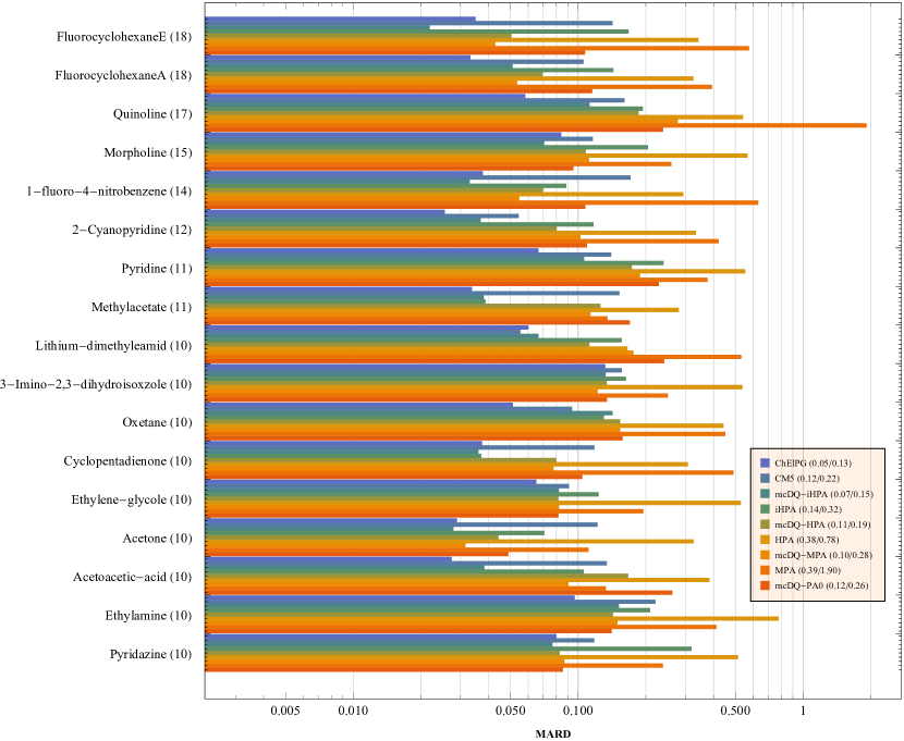
Figure 3: The MARD (Eq. (5)) of various PACs schemes for a subset of molecule taken from ref. ²⁰. Numbers in parenthesis appearing near the molecule names indicate the number of atoms in that molecule. The pair of numbers (median/max) appearing in the legend box near each scheme is, respectively, the median and maximum of the relative deviance taken over the shown set molecules.

In Table 1 we show, for each set of PACs the magnitude of the charge correction $\left\|\Delta q\right\|_{\infty}$. For a given molecule the mcD correction is largest for 0PA and then for MPA and HPA and it is smallest for iHPA. mcDQ corrections are in general considerably larger than mcD but in both methods $\left\|\Delta q\right\|_{\infty}$ decreases as the number of atoms in the molecule grows. This is due to the fact that in large systems even small charge shifts have a large affect on the dipole and the quadrupole moments.

Molecule	Sym	$A$	$F$	$C$	$\left\|\Delta q\right\|_{\infty}$ (mcD)								$\left\|\Delta q\right\|_{\infty}$ (mcDQ)
					0PA		MPA		HPA		iHPA		0PA		MPA		HPA		iHPA
Pyridazine	$C_{2v}$	10	7	6	0.	11	0.	02	0.	06	0.	04	0.	27	0.	29	0.	17	0.	12
Ethylamine	$C_{s}$	10	7	6	0.	04	0.	01	0.	03	0.	01	1.	17	1.	61	1.	22	1.	28
Acetoacetic acid	$C_{1}$	10	9	6	0.	07	0.	02	0.	03	0.	01	0.	54	0.	26	0.	25	0.	21
Acetone	$C_{2v}$	10	5	5	0.	17	0.	02	0.	05	0.	01	0.	52	0.	48	0.	34	0.	08
Ethylene-glycol	$C_{1}$	10	10	9	0.	09	0.	03	0.	05	0.	02	0.	67	0.	88	0.	64	0.	54
Cyclopentadienone	$C_{2v}$	10	6	6	0.	09	0.	04	0.	03	0.	00	0.	19	0.	22	0.	05	0.	02
Oxetane	$C_{s}$	10	7	6	0.	08	0.	05	0.	03	0.	01	1.	09	1.	29	1.	09	1.	09
3-Imino-2,3-dihydroisoxzole	$C_{s}$	10	8	6	0.	05	0.	02	0.	02	0.	01	0.	79	0.	83	0.	69	0.	41
Lithium-dimethylamine	$C_{2v}$	10	6	4	0.	31	0.	16	0.	05	0.	04	0.	31	0.	16	0.	05	0.	04
Methylacetate	$C_{s}$	11	9	6	0.	10	0.	02	0.	02	0.	01	0.	53	0.	22	0.	26	0.	01
Pyridine	$C_{2v}$	11	7	4	0.	06	0.	02	0.	03	0.	01	0.	15	0.	23	0.	09	0.	03
2-Cyanopyridine	$C_{s}$	12	12	6	0.	12	0.	05	0.	04	0.	01	0.	19	0.	19	0.	07	0.	03
1-fluoro-4-nitrobenzene	$C_{2v}$	14	9	6*	0.	05	0.	06	0.	01	0.	01	0.	13	0.	20	0.	05	0.	04
Morpholine	$C_{s}$	15	9	6	0.	03	0.	01	0.	02	0.	01	0.	47	0.	04	0.	33	0.	08
Quinoline	$C_{s}$	17	17	6	0.	03	0.	12	0.	02	0.	01	0.	10	0.	26	0.	05	0.	02
Fluorocyclohexane (A)	$C_{s}$	18	12	6	0.	05	0.	03	0.	02	0.	01	0.	17	0.	06	0.	05	0.	02
Fluorocyclohexane (E)	$C_{s}$	18	12	6	0.	04	0.	03	0.	01	0.	01	0.	17	0.	08	0.	07	0.	04
Median					0.	07	0.	03	0.	03	0.	01	0.	31	0.	23	0.	17	0.	04
Max					0.	31	0.	16	0.	06	0.	04	1.	17	1.	61	1.	22	1.	28

Table 1: The PAC change $\left\|\Delta q\right\|_{\infty}=max_{1\leq a\leq A}\left|\Delta q_{a}\right|$ induced by mcD and mcDQ for 0PA (where the reference PACs are all zero), MPA, HPA and iHPA for the set of molecules of Fig. 3. Also shown the number of atoms $A$ the number of degrees of freedom $F$ and the number of constraints $C$ for each molecule.

In table 2 we summarize the MARD statistics (median and maximal) for for four sets of reference charges: 0PA (reference charges are equal to zero) and MPA, HPA, iHPA. The efficiency of the mc procedure is apparent for MPA, HPA and iHPA, where the mcD reduces the median/maximal MARD by about a factor of 2. mcDQ reduces the MARD further, by a factor of 3 for 0PA and ~2 for MPA and HPA and only 1.1 for iHPA. We thus see that iHPA reconstruction of the ESP strongly benefits from a dipole correction and, interestingly, much less a quadrupole correction.

	0PA	MPA	HPA	iHPA
no-correction	NA	0.39/1.90	0.38/0.78	0.14/0.32
mcD	0.41/0.67	0.18/0.60	0.18/0.53	0.08/0.17
mcDQ	0.12/0.26	0.10/0.28	0.11/0.19	0.07/0.15

Table 2: The median/maximal MARD (for the set of molecules used above) determined for each PAC reference found for: non-corrected, and minimally-corrected schemes, mcD and mcDQ .

PACs are sometimes used when molecules distort. In this case, it is important that the they remain continuous under the distortion, so as to enable force calculations. The MPA/HPA/iHPA do not show non-smooth behavior and the mcDQ which is a minimization procedure does not show it as well. In 4 we show the MPA, mcDQ-MPA and ChElPG PACs of the oxygen atom in N-methylethanamide³⁰ the as a function of the dihedral angle $\phi$. It is seen that as the angle increases from 0 the mcDQ-MPA PAC slightly decreases and then increase rapidly followed by a rapid yet continuous drop near $\phi_{c}=0.25$ from a value of $q_{O}=-0.25$ to $q_{O}\approx-0.64$. An additional very sharp feature is seen near $\phi=\pi$. We have checked that this sharp feature is not discontinuous (see inset in Fig. 4) and that the matrix $S$ of Eq. 23 does not become rank deficient. Similar behavior is seen for the PACs of other atoms. We thus conclude that the charges change continuously although sometimes very rapid charge fluctuations can occur.

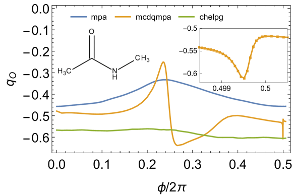
Figure 4: The partial charge, determined by MPA, mcDQ-MPA and ChElPG on the oxygen atom as a function of the O-C-N-H dihedral angle $\phi$ in N-methylethanamide (NMA). Inset om the right shows the sharp feature near $\phi=\pi$.

4 Summary and conclusions

We have studied a new scheme for minimally correcting reference PACs so that they reproduce the exact dipole and quadrupole moments of a molecule and we found that such a minimal correction greatly improves the correlation of the PAC-ESP with respect to the MOL-ESP. The minimal correction scheme does not alter symmetry properties of the reference PACs. Hence, minimally-corrected PACs (mc-PACs) based on MPA, HPA, iHPA fully respect the point-symmetry and rotational/translational symmetries of the molecule.

An additional benefit of the mc-PACs is their stability for inner (or buried) atoms of large molecules. This rises from the stability of the standard population schemes themselves and the fact that mc-PACs involve rather small corrections. As an example, consider the 2-(Dimethylamino)-2-propanol molecule:

for which the ChElPG, HPA and mcDQ-HPA PACs are shown in Fig. 5. Here, ChElPG tends to polarize the molecule: the oxygen and nitrogen share between them a negative unit charge and this is counteracted by the positive unit charge of the central carbon atom C3. On the other hand, MPA assigns a low charge for C3 and spreads rather evenly the remaining positive charge on the 12 terminal hydrogen atoms. mc-MPA charges are very close to those of MPA and thus yet they improve significantly the ESP description for this molecule: the MPA MARD is 0.35 while that of the mc-MPA is 0.1. It is worthwhile to note that the PACs assigned by ChElPG also have a MARD of 0.1.

When the underlying reference is the iHPA set of PACs the resulting ESP is of similar quality to that of the ChElPG set of PACs resulting from a best-fit to ESPs. The dependence of the PACs on the molecular distortion was demonstrated to have sometimes very sharp features however all the changes were smooth, hence forces can be calculated on the atoms of the molecule.

The method here bears a similarity to the optimal point-charge model of Ref. ¹⁰ which determines PACs that reproduce as many low-order moments as possible. The crucial difference is best seen when systems grow, model of Ref. ¹⁰ would target increasingly higher electrostatic moments as more atoms are included while the present method targets multipoles up to second order and not beyond, thereby avoiding the numerical instabilities described in see Ref. ¹¹. On the other hand. the optimal point-charge model treats the multipole constraints in a more systematic way by minimizing the error over unused moments in the last incomplete spherical shell.

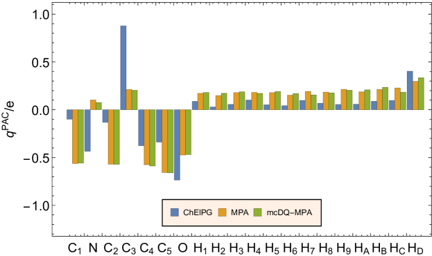
Figure 5: The ChElPG, MPA and mc-MPA PACs for the 2-(Dimethylamino)-2-propanol

References

- Lifson and Warshel 1968 Lifson, S.; Warshel, A. J. Chem. Phys. 1968, 49, 5116
- Warshel and Levitt 1976 Warshel, A.; Levitt, M. J. Mol. Biol. 1976, 103, 227–249
- Allinger et al. 1989 Allinger, N. L.; Yuh, Y. H.; Lii, J. H. J. Am. Chem. Soc. 1989, 111, 8551–8566
- Field et al. 1990 Field, M. J.; Bash, P. A.; Karplus, M. J. Comput. Chem. 1990, 11, 700–733
- Duffy and Jorgensen 2000 Duffy, E. M.; Jorgensen, W. L. J. Am. Chem. Soc. 2000, 122, 2878–2888
- Politzer and Truhlar 2013 Politzer, P.; Truhlar, D. G. Chemical applications of atomic and molecular electrostatic potentials: reactivity, structure, scattering, and energetics of organic, inorganic, and biological systems; Springer Science & Business Media, 2013
- Mei et al. 2015 Mei, Y.; Simmonett, A. C.; Pickard, F. C.; DiStasio, R.; Brooks, B. R.; Shao, Y. J. Phys. Chem. A 2015,
- Jackson 1999 Jackson, J. D. Classical Electrodynamics, 3rd ed.; Wiley: New York, 1999
- Verstraelen et al. 2016 Verstraelen, T.; Vandenbrande, S.; Heidar-Zadeh, F.; Vanduyfhuys, L.; Van Speybroeck, V.; Waroquier, M.; Ayers, P. W. arXiv preprint arXiv:1608.05556 2016,
- Simmonett et al. 2005 Simmonett, A. C.; Gilbert*, A. T.; Gill, P. M. Mol. Phys. 2005, 103, 2789–2793
- Gilbert and Gill 2006 Gilbert, A.; Gill, P. Mol. Simul. 2006, 32, 1249–1253
- Mulliken 1955 Mulliken, R. S. J. Chem. Phys. 1955, 23, 1833–1840
- Löwdin 1950 Löwdin, P.-O. J. Chem. Phys. 1950, 18, 365–375
- Hirshfeld 1977 Hirshfeld, F. Theor. Chim. Acta 1977, 44, 129–138
- Foster and Weinhold 1980 Foster, J.; Weinhold, F. J. Am. Chem. Soc. 1980, 102, 7211–7218
- Singh and Kollman 1984 Singh, U. C.; Kollman, P. A. J. Comput. Chem. 1984, 5, 129–145
- Bultinck et al. 2007 Bultinck, P.; Van Alsenoy, C.; Ayers, P. W.; Carbó-Dorca, R. J. Chem. Phys. 2007, 126, 144111
- Bultinck et al. 2009 Bultinck, P.; Cooper, D. L.; Van Neck, D. Phys. Chem. Chem. Phys. 2009, 11, 3424–3429
- Van Damme et al. 2009 Van Damme, S.; Bultinck, P.; Fias, S. J. Chem. Theory Comput. 2009, 5, 334–340
- Marenich et al. 2012 Marenich, A. V.; Jerome, S. V.; Cramer, C. J.; Truhlar, D. G. J. Chem. Theory Comput. 2012, 8, 527–541
- Breneman and Wiberg 1990 Breneman, C. M.; Wiberg, K. B. J. Comput. Chem. 1990, 11, 361–373
- Chirlian and Francl 1987 Chirlian, L. E.; Francl, M. M. J. Comput. Chem. 1987, 8, 894–905
- Momany 1978 Momany, F. A. J. Phys. Chem. 1978, 82, 592–601
- Besler et al. 1990 Besler, B.; Merz Jr, K.; Kollman, P. J. Comput. Chem 1990, 11, 431–439
- Bayly et al. 1993 Bayly, C. I.; Cieplak, P.; Cornell, W.; Kollman, P. A. J. Phys. Chem. 1993, 97, 10269–10280
- Cornell et al. 1993 Cornell, W. D.; Cieplak, P.; Bayly, C. I.; Kollmann, P. A. J. Am. Chem. Soc. 1993, 115, 9620–9631
- Williams 1988 Williams, D. E. J. Comput. Chem. 1988, 9, 745–763
- Sigfridsson and Ryde 1998 Sigfridsson, E.; Ryde, U. Journal of Computational Chemistry 1998, 19, 377–395
- Laio et al. 2002 Laio, A.; VandeVondele, J.; Rothlisberger, U. J. Phys. Chem. B 2002, 106, 7300–7307
- Hu et al. 2007 Hu, H.; Lu, Z.; Yang, W. J. Chem. Theory Comput. 2007, 3, 1004–1013
- Francl and Chirlian 2000 Francl, M. M.; Chirlian, L. E. Rev. Comput. Chem. 2000, 14, 1–31
- Jakobsen and Jensen 2016 Jakobsen, S.; Jensen, F. Journal of chemical theory and computation 2016, 12, 1824–1832
- Shao et al. 2015 Shao, Y. et al. Mol. Phys. 2015, 113, 184–215
- Zhao and Truhlar 2006 Zhao, Y.; Truhlar, D. G. The Journal of chemical physics 2006, 125, 194101
- Lynch et al. 2003 Lynch, B. J.; Zhao, Y.; Truhlar, D. G. The Journal of Physical Chemistry A 2003, 107, 1384–1388
- Golub and van Loan 1996 Golub, G. H.; van Loan, C. F. Matrix Computations, 3rd ed.; The John Hopkins University Press: Baltimore, 1996