Cosmic Rays in Intermittent Magnetic Fields

Abstract

The propagation of cosmic rays in turbulent magnetic fields is a diffusive process driven by the scattering of the charged particles by random magnetic fluctuations. Such fields are usually highly intermittent, consisting of intense magnetic filaments and ribbons surrounded by weaker, unstructured fluctuations. Studies of cosmic ray propagation have largely overlooked intermittency, instead adopting Gaussian random magnetic fields. Using test particle simulations, we calculate cosmic ray diffusivity in intermittent, dynamo-generated magnetic fields. The results are compared with those obtained from non-intermittent magnetic fields having identical power spectra. The presence of magnetic intermittency significantly enhances cosmic ray diffusion over a wide range of particle energies. We demonstrate that the results can be interpreted in terms of a correlated random walk.

Introduction

Cosmic rays are charged relativistic particles (mostly protons) scattered, as they propagate, by random magnetic fields (Berezinskii et al., 1990). Over sufficiently long time and length scales, their propagation is diffusive (Cesarsky, 1980). Assuming an interstellar magnetic field of strength $5\,\mu{\rm G}$, the Larmor radius $r_{\text{L}}$ of a cosmic ray proton of energy $5\,{\rm GeV}$ is of order $10^{12}\,{\rm cm}$, much smaller than the correlation length of interstellar MHD turbulence ($\sim 10^{20}\,{\rm cm}$). Thus, cosmic rays closely follow field lines (for a significant time) and so the geometry and statistical properties of magnetic fields control their propagation. The dominant contribution to particle scattering is from magnetic irregularities at a scale comparable to $r_{\text{L}}$. In this paper, we mostly discuss cosmic rays that propagate diffusively.

With exceptions discussed below (see also Alouani-Bibi & le Roux, 2014; Pucci et al., 2016), studies of cosmic ray propagation employ random magnetic fields with Gaussian statistics that are completely described by the two-point correlation function or the power spectrum (e.g., Michalek & Ostrowski, 1997; Giacalone & Jokipii, 1999; Casse et al., 2002; Parizot, 2004; Candia & Roulet, 2004; DeMarco et al., 2007; Globus et al., 2008; Plotnikov et al., 2011; Harari et al., 2014; Snodin et al., 2016; Subedi et al., 2017). However, the interstellar and intergalactic magnetic fields have a more complicated structure. The fluctuation (small-scale) dynamo (Zeldovich et al., 1990; Wilkin et al., 2007) and random shock waves (Bykov & Toptygin, 1987) produce highly intermittent, strongly non-Gaussian, essentially three-dimensional magnetic fields with random magnetic filaments and ribbons surrounded by weaker fluctuations. Filamentary and planar structures in the interstellar medium, consistent with the notion of spatial intermittency, have been detected in the radio (Sect. 5.2 in Haverkorn & Spangler, 2013) and sub-millimeter (Zaroubi et al., 2015) ranges as well as in the neutral hydrogen distribution (Heiles & Troland, 2005). In such a magnetic field, the propagation of charged particles is controlled not only by its power spectrum, but also by the size and separation of the magnetic structures. The influence of such a complex magnetic field upon cosmic ray propagation is poorly understood. Existing theories, on the quasilinear approach (Jokipii, 1966; Schlickeiser, 2002; Berezinskii et al., 1990), or its nonlinear extensions and alternative ideas (e.g., Matthaeus et al., 2003; Shalchi, 2009; Yan & Lazarian, 2002; Vlad et al., 1998), do not consider intermittency, or use the Corrsin hypothesis (Corrsin, 1959), which assumes Gaussian statistics for the magnetic field. Recent test particle simulations used magnetic fields obtained from simulations of MHD turbulence (e.g., Dmitruk et al., 2004; Reville et al., 2008; Beresnyak et al., 2011; Lynn et al., 2012; Weidl et al., 2015; Cohet & Marcowith, 2016) (see also Roh et al., 2016). These models are free from the assumption of Gaussian statistics but they do not consider any effects of magnetic structures even if those were present. There have been no systematic attempts to examine the significance of realistic, physically realizable magnetic intermittency in 3D; this is our goal here. In intermittent magnetic fields, particle trapping can be important even in 3D. We note that the Kubo number, often used to delineate different transport regimes, depends only on second-order correlations and is therefore insensitive to intermittency.

We use test particle simulations (Giacalone & Jokipii, 1999; Casse et al., 2002; Desiati & Zweibel, 2014; Snodin et al., 2016), integrating the equation of motion for a large number of particles in a statistically isotropic, prescribed magnetic field, in the regime where cosmic ray pressure is too low to excite significant MHD waves. The magnetic field is obtained as a solution of the induction equation with a prescribed velocity field that drives the fluctuation dynamo. This produces a realistic, intermittent magnetic field. The degree of intermittency depends on the magnetic Reynolds number $R_{\mathrm{m}}$. As $R_{\mathrm{m}}$ increases, the magnetic structures occupy a smaller proportion of the volume. The intermittency introduces two distinct particle propagation regimes, one within a magnetic structure and another between them. Cosmic ray particles are strongly scattered by the magnetic structures and move relatively freely between them. By comparing particle diffusion in an intermittent field with that in a magnetic field lacking structure, but with identical power spectrum, we demonstrate that intermittency can significantly enhance diffusion, and so diffusion cannot be described in terms of the power spectrum alone.

Magnetic Field Produced by Dynamo Action

We generate intermittent, statistically isotropic, fully three-dimensional random magnetic fields $\mathbf{b}$ by solving the induction equation with a prescribed velocity field $\mathbf{u}$,

$$\frac{\partial\mathbf{b}}{\partial t}=\nabla\times(\mathbf{u}\times\mathbf{b})+R_{\mathrm{m}}^{-1}\nabla^{2}\mathbf{b},\qquad\nabla\cdot\mathbf{b}=0,$$ (1)

with periodic boundary conditions in a cubic domain of width $L=2\pi$ and $256^{3}$ or $512^{3}$ mesh points. Equation (1) is written in a dimensionless form, expressing length in the units of the flow scale $l_{0}$ and time in the units of $l_{0}/u_{0}$, where $u_{0}$ is the rms flow speed. Here $R_{\mathrm{m}}=l_{0}u_{0}/\eta$ is the magnetic Reynolds number and $\eta$ is the magnetic diffusivity, assumed to be constant. In a generic, three-dimensional, random flow, dynamo action occurs (i.e., the mean magnetic energy density grows exponentially with $t$) provided $R_{\mathrm{m}}>R_{\mathrm{m,c}}$, where $R_{\mathrm{m,c}}$ is the critical magnetic Reynolds number (Zeldovich et al., 1990). Depending on the nature of the velocity field, typically $R_{\mathrm{m,c}}\simeq 10$–$100$, and the magnetic field decays for $R_{\mathrm{m}}<R_{\mathrm{m,c}}$ (Brandenburg & Subramanian, 2005). As $R_{\mathrm{m}}\to\infty$, the magnetic structures produced by the dynamo become progressively more filamentary in nature, with the thickness of each filament of the order of $d=l_{0}R_{\mathrm{m}}^{-1/2}$, and a characteristic filament length (radius of curvature) of the order of $l_{0}$ (Zeldovich et al., 1990; Wilkin et al., 2007). The magnetic field used in our simulations is an eigenfunction obtained by renormalizing the exponentially growing solution of Eq. (1) to have a constant rms field strength $b_{0}$. We expect the magnetic structure of the corresponding nonlinear dynamo to be similar to that of the marginal eigenfunction obtained at $R_{\mathrm{m}}\approx R_{\mathrm{m,c}}$ (Subramanian, 1999). However, we consider a wider range of $R_{\mathrm{m}}$ to explore the effects of a variable degree of intermittency: it increases with $R_{\mathrm{m}}$.

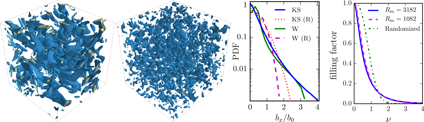
Figure 1.— Isosurfaces of magnetic field strength $b^{2}/b_{0}^{2}=2.5$ (blue) and $b^{2}/b_{0}^{2}=5$ (yellow) with $b_{0}$ the rms magnetic field, for magnetic field generated by the KS flow (3) at $R_{\mathrm{m}}=1082$ (left) and for the same magnetic field after Fourier phase randomization as described in the text (second from left). Magnetic field generated by the W flow (2) is similarly affected (not shown). The second from right panel shows the PDFs of a magnetic field component $b_{x}$ for the original (KS,W: solid) and randomized [KS (R), W (R): dashed] magnetic fields obtained with both velocity fields (only $b_{x}>0$ is show as the PDFs are essentially symmetric about $b_{x}=0$). The randomized fields have almost perfectly Gaussian statistics, whereas magnetic intermittency leads to heavy tails. The panel on the right shows the fractional volume within magnetic structures where $b\geq\nu b_{0}$, with $b_{0}$ the rms field strength, as a function of $\nu$ for the intermittent magnetic field produced by the flow (3) (solid for $R_{\mathrm{m}}=3182$ and dashed for $R_{\mathrm{m}}=1082$) and its Gaussian counterpart (dash-dotted, for $R_{\mathrm{m}}=3142$ and $1082$) obtained by Fourier phase randomization; the filling factor of the randomized fields is independent of $R_{\mathrm{m}}$.

To isolate robust features of cosmic ray propagation independent of the particular form of intermittent magnetic field, we use two types of incompressible flow to drive the dynamo, both chaotic, but one of a single scale, and the other multi-scale with a controlled power spectrum. The first flow (Willis, 2012), henceforth referred to as flow W, is stationary,

$$\mathbf{u}(\mathbf{x})=(2/\sqrt{3})(\sin y\cos z,\sin z\cos x,\sin x\cos y).$$ (2)

It is a very efficient dynamo with $R_{\mathrm{m,c}}\approx 11$, producing regularly spaced magnetic structures in the form of ellipsoids of identical size that become thinner as $R_{\mathrm{m}}$ increases and whose positions are determined solely by the flow geometry (so are independent of $R_{\mathrm{m}}$). The second flow (KS) is time-dependent and multi-scale; it was employed for dynamo simulations (Wilkin et al., 2007) and as a Lagrangian model of turbulence (Fung et al., 1992):

$$\mathbf{u}(\mathbf{x},t)=\sum_{n=0}^{N-1}\left(\mathbf{C}_{n}\cos\phi_{n}+\mathbf{D}_{n}\sin\phi_{n}\right),$$ (3)

where $\phi_{n}=\mathbf{k}_{n}\cdot\mathbf{x}+\omega_{n}t$, with $\mathbf{k}_{n}$ a randomly oriented wave vector (of magnitude $k_{n}$) and $\omega_{n}$ a frequency specified below. The random vectors, $\mathbf{C}_{n}$ and $\mathbf{D}_{n}$, are chosen to be orthogonal to $\mathbf{k}_{n}$ to ensure $\nabla\cdot\mathbf{u}=0$. We select $N=40$ distinct wave vectors, with magnitudes between $k_{0}=2\pi/L$ and $k_{N-1}\approx 8k_{0}$, so that the flow is periodic with the outer scale $l_{0}=L$. The amplitudes of $\mathbf{C}_{n}$ and $\mathbf{D}_{n}$ are selected to produce an energy spectrum $E(k)\propto k^{-5/3}$ with $\int_{k_{0}}^{k_{N-1}}E(k)dk=u_{0}^{2}/2$. We take $\omega_{n}=[k_{n}^{3}E(k_{n})]^{1/2}$, which introduces a scale-dependent time variation. The dynamo in this flow has $R_{\mathrm{m,c}}\approx 1000$ (Wilkin et al., 2007). The flow produces transient magnetic structures, consisting of filaments of various sizes, as illustrated in the leftmost panel of Fig. 1.

To identify the effect of magnetic intermittency on cosmic ray diffusion, we also consider random magnetic fields where the structures have been destroyed but the magnetic energy spectrum remains unchanged (Snodin et al., 2013). This is achieved by taking the spatial Fourier transform of $\mathbf{b}(\mathbf{x})$ from Eq. (1), and then multiplying each complex Fourier mode by $\exp[\mathrm{i}\psi(\mathbf{k})]$, with $\psi(\mathbf{k})$ a random phase selected independently for each $\mathbf{k}$. The inverse Fourier transform of the result produces a magnetic field with an unchanged spectrum but with little remaining structure, as demonstrated in the second from left panel of Fig. 1. As shown on the second from right panel of Fig. 1, the probability density functions (PDFs) of the field components for the intermittent fields produced by each flow (W and KS) have long, heavy tails, while the phase randomization produces nearly Gaussian random fields. Another aspect of this difference is also illustrated in the rightmost panel of Fig. 1 where the fractional volume occupied by magnetic structures with $b/b_{0}>\nu$ is shown as a function of $\nu$: an intermittent magnetic field has more strong, localized structures with $\nu\gtrsim 1.4$ than a Gaussian field with identical power spectrum.

To explore the effects of a mean magnetic field, we also consider particle propagation in a magnetic field given by $\mathbf{B}=\mathbf{b}+\mathbf{B}_{0}$, where $\mathbf{B}_{0}$ is an imposed uniform magnetic field. In such cases, the rms magnetic field $\tilde{b}_{0}$ quoted below includes the mean part, $\tilde{b}_{0}^{2}=B_{0}^{2}+b_{0}^{2}$.

Cosmic Ray Propagation

Using magnetic field realizations generated from Eq. (1), or the corresponding randomized magnetic fields, we obtain an ensemble of cosmic ray trajectories ($\geq 1000$ in number) by solving numerically the dimensionless equation of motion for the particle trajectories $\mathbf{x}(t)$,

$$\ddot{\mathbf{x}}=\alpha\dot{\mathbf{x}}\times\mathbf{B}(\mathbf{x}),$$ (4)

with $\alpha=ql_{0}\tilde{b}_{0}/(\gamma mcv_{0})$, $q$ the particle charge, $m$ its rest mass, $\tilde{b}_{0}$ the total rms field strength,$\gamma$ the Lorentz factor, $v_{0}$ the particle speed and $c$ the speed of light. As in most cosmic ray propagation models (Berezinskii et al., 1990; Schlickeiser, 2002; Shalchi, 2009), we neglect electric fields in Eq. (4): they are negligible at the scales of interest ($\simeq 1\,{\rm kpc}$ in galaxies and $\simeq 10\,{\rm kpc}$ in galaxy clusters). Hence, the particle speed $v_{0}$ remains constant. Each particle is given a random initial position and propagation direction, but the same initial speed. The characteristic dimensionless Larmor radius, based on the rms magnetic field strength, is $r_{\text{L}}/l_{0}=\alpha^{-1}$; we use this ratio to characterize the particle properties. When $B_{0}=0$, we calculate the isotropic diffusion coefficient $\kappa=\lim_{t\to\infty}\langle|\Delta\mathbf{x}(t)|^{2}\rangle/(6t)$, where $\Delta\mathbf{x}(t)$ is the particle displacement, and the angular brackets denote averaging over particle displacements. In the presence of a mean magnetic field directed along the $z$-axis, we introduce similarly defined parallel and perpendicular diffusion coefficients, $\kappa_{\parallel}=\lim_{t\to\infty}\langle\Delta z(t)^{2}\rangle/(2t)$ and $\kappa_{\perp}=\lim_{t\to\infty}\langle[\Delta x(t)^{2}+\Delta y(t)^{2}]\rangle/(4t)$.

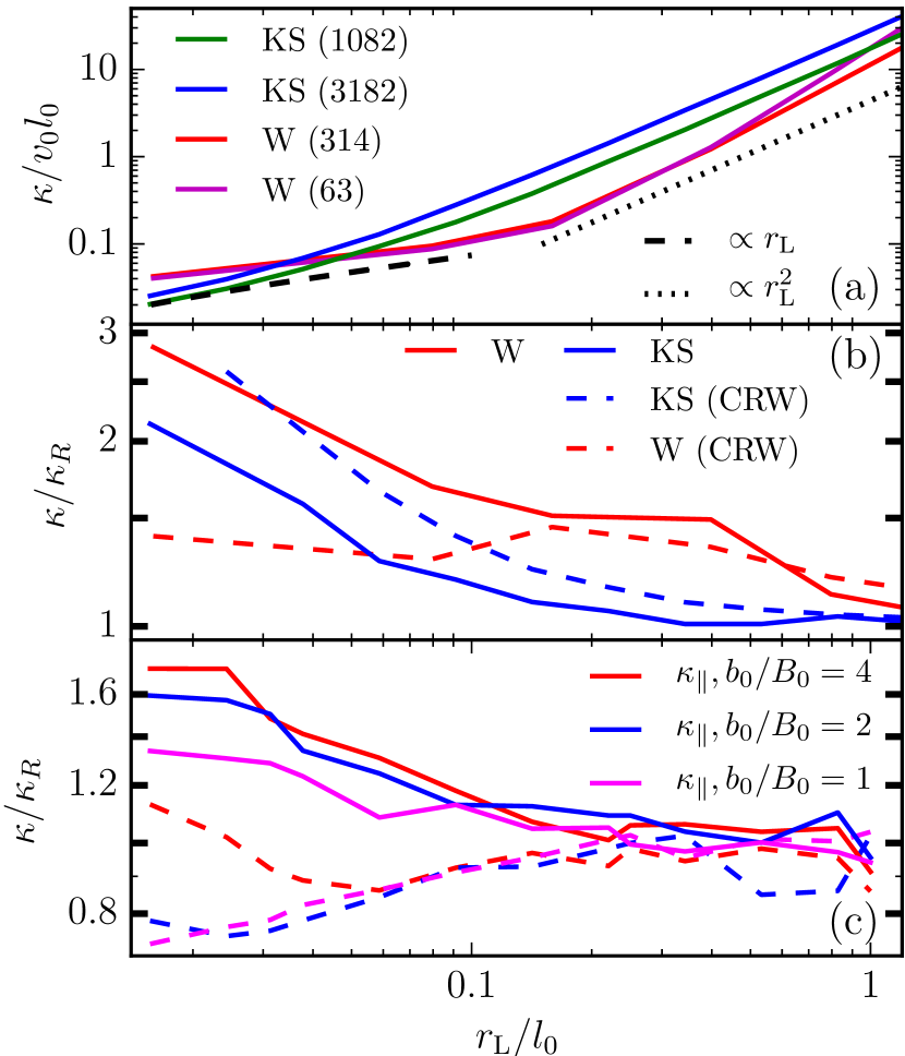
Figure 2.— (a) The cosmic ray diffusion coefficient for the W flow (2) (red, magenta) and the KS flow (3) (blue, green) as a function of $r_{\text{L}}/l_{0}$ for the values of $R_{\mathrm{m}}$ given in parenthesis in the legend. The dotted and dashed line shows the scaling $\kappa\propto r_{\text{L}}^{2}$ and $\kappa\propto r_{\text{L}}$ respectively. (b) The ratio of diffusion coefficients from intermittent, $\kappa$, and randomized, $\kappa_{\mathrm{R}}$, magnetic fields for the two flows (solid lines, KS with $R_{\mathrm{m}}=3182$, W with $R_{\mathrm{m}}=314$). The dashed lines of same color show the corresponding CRW model, Eq. (7). (c) As in (b) but in the presence of a mean magnetic field $B_{0}$, of the relative strength specified in the legend, for the KS flow with $R_{\mathrm{m}}=3182$; $\kappa_{\parallel}$ and $\kappa_{\perp}$ are shown solid and dashed, respectively.

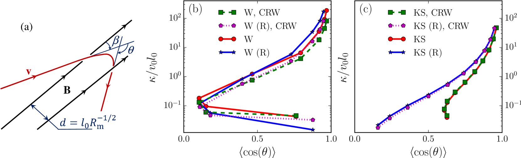
Figure 3.— (a) A charged particle with the pitch angle $\beta$ is deflected by an angle $\theta$ in a magnetic structure of a thickness $d$, thus introducing correlation into the random particle trajectory. The dependence of the diffusivity in simulations on $\langle\cos\theta\rangle$ in the W flow and the randomized (R) magnetic field is shown in (b) (solid lines). The corresponding CRW approximations (Eq. (7)) are shown with broken lines. (c) is as in (b), but for the KS flow. These results are obtained for $B_{0}=0$.

Cosmic Ray Diffusivity

Figure 2a shows the dependence of the cosmic ray diffusion coefficient on $r_{\text{L}}/l_{0}$ (proportional to the particle energy) for $B_{0}=0$. For $r_{\text{L}}/l_{0}\gg 1$, we recover the asymptotic scaling $\kappa\propto r_{\text{L}}^{2}$ (high energy limit) in agreement with earlier results (Parker, 1965; Aloisio & Berezinsky, 2004; Parizot, 2004; Globus et al., 2008; DeMarco et al., 2007; Beresnyak et al., 2011; Plotnikov et al., 2011; Harari et al., 2014; Snodin et al., 2016; Subedi et al., 2017). At lower energies, the dependence of $\kappa$ on particle energy is weaker and is sensitive to magnetic structure. Magnetic intermittency is expected to be important at those energies where

$$r_{\text{L}}/l_{0}\lesssim 1,$$ (5)

and the dependence $\kappa(r_{\text{L}}/l_{0})$ in Fig. 2a indeed deviates from the asymptotic form in this range. The role of magnetic intermittency is demonstrated in Fig. 2b, showing the ratio of the diffusivity $\kappa$ calculated with a dynamo generated magnetic field to that in the corresponding randomized field, $\kappa_{\mathrm{R}}$ ($B_{0}=0$ in Panels a and b). At high energies (large $r_{\text{L}}/l_{0}$), $\kappa/\kappa_{\mathrm{R}}\simeq 1$, suggesting that the magnetic structures play little role. However, $\kappa/\kappa_{\mathrm{R}}$ increases rapidly up to more than $2.5$ at lower energies: magnetic structures enhance diffusion when inequality (5) is satisfied. We find that the ratio $\kappa/\kappa_{\mathrm{R}}$ at fixed $r_{\text{L}}/l_{0}$ increases with $R_{\mathrm{m}}$ for a given flow. At high values of $r_{\text{L}}/l_{0}$, the diffusivity still depends on $R_{\mathrm{m}}$ via changes in the magnetic correlation length (Fig. 2a), but not via the $R_{\mathrm{m}}$-dependent intermittency, as suggested by Fig. 2b where $\kappa/\kappa_{R}$ tends to unity as $r_{\text{L}}/l_{0}$ increases. One might expect a change in the diffusivity behavior at $r_{\text{L}}/l_{0}\approx R_{\mathrm{m}}^{-1/2}$, associated with the thickness of magnetic filaments, and this may explain the variation in slope of $\kappa$ at low $r_{\text{L}}/l_{0}$ in Fig. 2a (or the ratios in Fig. 2b). However, at present the role of this scale is unclear.

Figure 2c illustrates the effects of the mean magnetic field, presenting the ratio of the parallel and perpendicular diffusivities in the intermittent and Gaussian magnetic fields. A mean magnetic field somewhat reduces the effect of intermittency, but does not eliminate it even for $b_{0}/B_{0}=1$. Magnetic intermittency enhances $\kappa_{\parallel}$ (i.e. $\kappa_{\parallel}>(\kappa_{\parallel})_{\mathrm{R}}$) at all but the highest energies, but $\kappa_{\perp}<(\kappa_{\perp})_{\mathrm{R}}$ at lower energies for $b_{0}/B_{0}=2$ and $b_{0}/B_{0}=1$. The effects of the mean field will be discussed in detail elsewhere.

Cosmic Ray Propagation as a Correlated Random Walk

The Brownian motion is a widely used model for diffusive processes. This is the simplest type of random walk where each step is made in a direction independent of the previous direction. In a continuum limit, it leads to the diffusion equation. However, a charged particle moves differently. As illustrated in Fig. 3a, the direction of its motion after deflection by a magnetic structure is correlated with the previous direction. The deflection angle $\theta$ is related to $r_{\text{L}}$, the angle between the velocity and magnetic field, $\beta$, and the magnetic structure width $d$,

$$\theta\simeq d/(r_{\text{L}}\sin\beta).$$ (6)

This is a correlated random walk (CRW) (Gillis, 1955), a first-order Markov chain (since the correlation does not extend beyond two consecutive steps). For a symmetric probability distribution of $\theta$, the CRW diffusivity depends on $\langle\cos\theta\rangle$, where angular brackets denote the ensemble average. The mean-square displacement in the CRW was obtained in 2D (Kareiva & Shigesada, 1983), and implies the following 3D diffusivity (Eq. (3.3.7) in Chen & Renshaw, 1992):

$$\kappa=\frac{\langle l^{2}\rangle}{6\tau}+\frac{\langle l\rangle^{2}}{3\tau}\frac{\langle\cos\theta\rangle}{1-\langle\cos\theta\rangle},$$ (7)

with $\tau=\langle l\rangle/v$, $v$ the particle speed and $l$ the step length. To calculate $\langle\cos\theta\rangle$, we assume that the pitch angle $\beta$ is uniformly distributed between $0$ and $\pi$. Defining $a=d/r_{\text{L}}\simeq l_{0}R_{\mathrm{m}}^{-1/2}/r_{\text{L}}$, it can be shown that

$$\langle\cos\theta\rangle =\pi^{-1}\int_{0}^{\pi}\cos\left({a}/{\sin\beta}\right)\mathrm{d}\beta$$

$$=1-\tfrac{1}{2}\pi a\left[J_{0}(a)\mathcal{H}_{-1}(a)-J_{-1}(a)\mathcal{H}_{0}(a)\right],$$ (8)

where $J_{n}(x)$ and $\mathcal{H}_{n}(x)$ are the Bessel and Struve functions (2.5.8.6 in Prudnikov et al., 1991). Finite length of the magnetic structures can be accounted for, but this represents a small correction and the integral cannot be taken analytically.

To derive $\langle\cos\theta\rangle$ in the simulations, the particle trajectories were sampled each local Larmor time; the sampling frequency does not affect the results much (cf. Codling & Hill, 2005; Rosser et al., 2013). $\langle\cos\theta\rangle$ computed using Eq. (Cosmic Ray Propagation as a Correlated Random Walk) and the same obtained from the simulations show reasonable qualitative agreement if we adopt $d=l_{0}R_{\mathrm{m}}^{-1/2}$ for the flow (2) and $d$ as the thickness of the magnetic structures calculated using the Minkowski functionals (Wilkin et al., 2007) for the flow (3).

Figure 3b,c shows the variation of $\kappa$ with $\langle\cos\theta\rangle$, where $\kappa$ is obtained numerically for both the intermittent and randomized magnetic fields, and in each case the corresponding $\kappa$ predicted from Eq. (7) is also shown. For $\tau$ in Eq. (7), we have used $r_{\text{L}}/v_{0}$, where $r_{\text{L}}$ is the local Larmor radius. The agreement is remarkably good for the flow (2) and excellent for the less regular magnetic field resulting from the flow (3). This confirms directly that the cosmic ray propagation is a CRW with the diffusivity given by Eq. (7). This applies to both intermittent and Gaussian random magnetic fields (see also Fig. 2b). We note that the first term in Eq. (7) dominates at large $r_{\text{L}}$.

Conclusions

We have demonstrated that cosmic ray propagation in random magnetic fields is affected by magnetic intermittency in the range of energies (5), or

$$\frac{E}{1\,{\rm GeV}}\lesssim 10^{9}\frac{l_{0}}{1\,{\rm kpc}}\,\frac{B}{1\,\mu{\rm G}}.$$

In the interstellar medium, $l_{0}\simeq 100\,{\rm pc}$ and $B\simeq 10\,\mu{\rm G}$ and for ultra-relativistic protons, this energy range is $E\lesssim 10^{9}\,{\rm GeV}$. In galaxy clusters, $l_{0}\simeq 10\,{\rm kpc}$, $B\simeq 2\,\mu{\rm G}$ and $E\lesssim 10^{10}\,{\rm GeV}$.

Assuming $R_{\rm m,eff}=R_{\mathrm{m,c}}=100$ in the interstellar medium, we might expect some effect at $r_{\text{L}}/l_{0}=0.1$, which would correspond to $10^{8}\,{\rm GeV}$ protons using the above values. Such an effect might produce a knee or spectral break in the cosmic ray energy spectrum near this energy. The influence of magnetic intermittency extends to below this energy (the effect of intermittency on cosmic ray diffusivity increases as energy decreases), but further investigation is needed to quantify this. Finally, we note that magnetic intermittency may also affect ultrahigh energy cosmic rays that propagate non-diffusively, and that their propagation can also be interpreted as a CRW.

References

- Aloisio & Berezinsky (2004) Aloisio, R., & Berezinsky, V. 2004, Astrophys. J., 612, 900
- Alouani-Bibi & le Roux (2014) Alouani-Bibi, F., & le Roux, J. A. 2014, Astrophys. J., 781, 93
- Beresnyak et al. (2011) Beresnyak, A., Yan, H., & Lazarian, A. 2011, Astrophys. J., 728, 60
- Berezinskii et al. (1990) Berezinskii, V. S., Bulanov, S. V., Dogiel, V. A., & Ptuskin, V. S. 1990, Astrophysics of Cosmic Rays (Amsterdam: North-Holland)
- Brandenburg & Subramanian (2005) Brandenburg, A., & Subramanian, K. 2005, Phys. Rep., 417, 1
- Bykov & Toptygin (1987) Bykov, A. M., & Toptygin, I. N. 1987, Astrophys. Space Sci., 138, 341
- Candia & Roulet (2004) Candia, J., & Roulet, E. 2004, J. Cosmol. Astropart. Phys., 10, 7
- Casse et al. (2002) Casse, F., Lemoine, M., & Pelletier, G. 2002, Phys. Rev. D, 65, 023002
- Cesarsky (1980) Cesarsky, C. J. 1980, Ann. Rev. Astron. Astrophys., 18, 289
- Chen & Renshaw (1992) Chen, A., & Renshaw, E. 1992, J. Appl. Probab., 29, 792
- Codling & Hill (2005) Codling, E., & Hill, N. 2005, J. Theor. Biol., 233, 573
- Cohet & Marcowith (2016) Cohet, R., & Marcowith, A. 2016, Astron. Astrophys., 588, A73
- Corrsin (1959) Corrsin, S. 1959, Advances in Geophysics, 6, 161
- DeMarco et al. (2007) DeMarco, D., Blasi, P., & Stanev, T. 2007, J. Cosmol. Astropart. Phys., 6, 027
- Desiati & Zweibel (2014) Desiati, P., & Zweibel, E. G. 2014, Astrophys. J., 791, 51
- Dmitruk et al. (2004) Dmitruk, P., Matthaeus, W. H., & Seenu, N. 2004, Astrophys. J., 617, 667
- Fung et al. (1992) Fung, J. C. H., Hunt, J. C. R., Malik, N. A., & Perkins, R. J. 1992, J. Fluid Mech., 236, 281
- Giacalone & Jokipii (1999) Giacalone, J., & Jokipii, J. R. 1999, Astrophys. J., 520, 204
- Gillis (1955) Gillis, J. 1955, Proc. Cambridge Philos. Soc., 51, 639
- Globus et al. (2008) Globus, N., Allard, D., & Parizot, E. 2008, Astron. Astrophys., 479, 97
- Harari et al. (2014) Harari, D., Mollerach, S., & Roulet, E. 2014, Phys. Rev. D, 89, 123001
- Haverkorn & Spangler (2013) Haverkorn, M., & Spangler, S. R. 2013, SSRv, 178, 483
- Heiles & Troland (2005) Heiles, C., & Troland, T. H. 2005, Astrophys. J., 624, 773
- Jokipii (1966) Jokipii, J. R. 1966, Astrophys. J., 146, 480
- Kareiva & Shigesada (1983) Kareiva, P. M., & Shigesada, N. 1983, Oecologia, 56, 234
- Lynn et al. (2012) Lynn, J. W., Parrish, I. J., Quataert, E., & Chandran, B. D. G. 2012, Astrophys. J., 758, 78
- Matthaeus et al. (2003) Matthaeus, W. H., Qin, G., Bieber, J. W., & Zank, G. P. 2003, Astrophys. J. Lett., 590, L53
- Michalek & Ostrowski (1997) Michalek, G., & Ostrowski, M. 1997, Astron. Astrophys., 326, 793
- Parizot (2004) Parizot, E. 2004, Nucl. Phys. B, Proc. Suppl., 136, 169
- Parker (1965) Parker, E. N. 1965, Planet. Space Sci., 13, 9
- Plotnikov et al. (2011) Plotnikov, I., Pelletier, G., & Lemoine, M. 2011, Astron. Astrophys., 532, A68
- Prudnikov et al. (1991) Prudnikov, A. P., Brychkov, Y. A., & Marichev, O. I. 1991, Integrals and Series: Elementary Functions (Vol. 1) (NY: Gordon & Breach)
- Pucci et al. (2016) Pucci, F., Malara, F., Perri, S., et al. 2016, Mon. Not. R. Astron. Soc., 459, 3395
- Reville et al. (2008) Reville, B., O’Sullivan, S., Duffy, P., & Kirk, J. G. 2008, Mon. Not. R. Astron. Soc., 386, 509
- Roh et al. (2016) Roh, S., Inutsuka, S.-i., & Inoue, T. 2016, Astropart. Phys., 73, 1
- Rosser et al. (2013) Rosser, G., Fletcher, A. G., Maini, P. K., & Baker, R. E. 2013, J. R. Soc. Interface, 10, 20130273
- Schlickeiser (2002) Schlickeiser, R. 2002, Cosmic Ray Astrophysics (Berlin: Springer)
- Shalchi (2009) Shalchi, A. 2009, Nonlinear Cosmic Ray Diffusion Theories (Berlin: Springer), doi:10.1007/978-3-642-00309-7
- Snodin et al. (2013) Snodin, A. P., Ruffolo, D., Oughton, S., Servidio, S., & Matthaeus, W. H. 2013, Astrophys. J., 779, 56
- Snodin et al. (2016) Snodin, A. P., Shukurov, A., Sarson, G. R., Bushby, P. J., & Rodrigues, L. F. S. 2016, Mon. Not. R. Astron. Soc., 457, 3975
- Subedi et al. (2017) Subedi, P., Sonsrettee. W., Blasi, P., et al. 2017, Accepted for publication in Astrophys. J., arXiv:1612.09507
- Subramanian (1999) Subramanian, K. 1999, Phys. Rev. Lett., 83, 2957
- Vlad et al. (1998) Vlad, M., Spineanu, F., Misguich, J. H., & Balescu, R. 1998, Phys. Rev. E, 58, 7359
- Weidl et al. (2015) Weidl, M. S., Jenko, F., Teaca, B., & Schlickeiser, R. 2015, Astrophys. J., 811, 8
- Wilkin et al. (2007) Wilkin, S. L., Barenghi, C. F., & Shukurov, A. 2007, Phys. Rev. Lett., 99, 134501
- Willis (2012) Willis, A. P. 2012, Phys. Rev. Lett., 109, 251101
- Yan & Lazarian (2002) Yan, H., & Lazarian, A. 2002, Phys. Rev. Lett., 89, 281102
- Zaroubi et al. (2015) Zaroubi, S., Jelić, V., de Bruyn, A. G., et al. 2015, Mon. Not. R. Astron. Soc., 454, L46
- Zeldovich et al. (1990) Zeldovich, Ya. B., Ruzmaikin, A. A., & Sokoloff, D. D. 1990, The Almighty Chance (Singapore: World Scientific)