Evidence for criticality in financial data

Abstract

We provide evidence that cumulative distributions of absolute normalized returns for the $100$ American companies with the highest market capitalization, uncover a critical behavior for different time scales $\Delta t$. Such cumulative distributions, in accordance with a variety of complex –and financial– systems, can be modeled by the cumulative distribution functions of $q$-Gaussians, the distribution function that, in the context of nonextensive statistical mechanics, maximizes a non-Boltzmannian entropy. These $q$-Gaussians are characterized by two parameters, namely $(q,\beta)$, that are uniquely defined by $\Delta t$. From these dependencies, we find a monotonic relationship between $q$ and $\beta$, which can be seen as evidence of criticality. We numerically determine the various exponents which characterize this criticality.

PACS numbers: 05.10.-a 71.45.Gm 89.65.Gh 05.45.Tp

The analysis of financial data by methods developed for physical systems, has extensively attracted the interest of physicists [1, 2, 3, 4, 5, 6, 7, 8, 9, 10, 11, 12]. In fact, financial markets are strongly fluctuating complex systems whose dynamics are difficult to understand because of the complexity of their internal elements and correlations, and also because of the many intractable external factors acting on them. However, remarkably enough, the interactions between these various ingredients generate many observables whose statistical properties appear to be similar for quite different markets. Consequently, we are allowed to refer to some “universal” trends, on which we focus herein.

As a matter of fact, it has been observed, in financial data, that rare events give raise to pronounced tails in the appropriate probability distributions — tails that are in fact frequently found in complex systems. Such is the case of the return distributions associated with time series [5, 13] on varying time scales, $\Delta t$. These fat tails reveal long-range correlations that frequently cause standard statistical mechanics to be inadequate for describing them. This kind of scenario also emerges in the systems that permanently reside in the neighborhood of their critical point, where physical quantities present power-law dependences of the type $f(x)\sim x^{-\tau}$, characterized by a critical exponent $\tau$.

Nonextensive statistical mechanics [14, 15], a current generalization of the Boltzmann-Gibbs (BG) statistical mechanics when its associated entropy $S_{BG}$ does not obey the standard asymptotic behavior $S_{BG}(N)\sim N$ for $N\to\infty$ ($N$ being the number of elements), occurs useful in the description of such complex finantial systems [16, 17, 18, 19, 20, 21].

This theory has been developed around the concept of nonadditive entropy, which is maximized, with the appropriate constraints [22], by the family of the $q$-Gaussian distributions

$$G_{q}(x)=A(q,\beta_{q})\exp_{q}[-\beta_{q}(x-\mu_{q})^{2}],$$ (1)

where $q$ is a characteristic index, $\beta_{q}$ is a sort of inverse temperature [23], $\mu_{q}$ is the Escort averaged fist moment [24], $A(q,\beta)$ is a normalization factor, and the function

$$\exp_{q}(x)\equiv[1+(1-q)x]_{+}^{1/(1-q)}$$ (2)

with $[x]_{+}=x$ if $x>0$ and $[x]_{+}=0$ otherwise, is a generalization of the exponential function — the $q\to 1$ limit makes $\exp_{q}(x)\to\exp(x)$ —. The normalization factor in eq. (1) reads [25], for the values of $q$ we are now involved ($1<q<3$):

$$A(q,\beta_{q})=\sqrt{\frac{q-1}{\pi}\beta_{q}}\frac{\Gamma\left[{\frac{1}{q-1}}\right]}{\Gamma\left[{\frac{3-q}{2\left({q-1}\right)}}\right]}.$$ (3)

The $q$-Gaussian distribution (1) generalizes the Gaussian distribution in a similar way as nonadditive entropy generalizes $S_{BG}$ [14]. In fact, the $q\to 1$ limit makes eqs. (1-3) to recover the Gaussian distribution, i.e., $G_{1}(x)=\frac{1}{\sigma_{1}\sqrt{2\pi}}\,\exp[\frac{(x-\mu_{1})^{2}}{2\sigma_{1}^{2}}]$. A generalization of the Central Limit Theorem, where the $q$-Gaussian distributions themselves become their attractors, has already been formulated [26, 27, 28].

In the present work, we follow along the lines of [29]. Namely, we apply a nonextensive statistical analysis to empirical distribution data of normalized returns in financial market. Our objective is to uncover some empirical laws that seem to govern such a financial markets.

The absolute normalized returns are conventionally defined in the following manner. For the time series $W(t)$ that represent the prizes — or the market index value — at time $t$, the returns over a sample interval $\Delta t$, $R_{\Delta t}(t)$, are defined as

$$R_{\Delta t}(t)\equiv\ln W(t+\Delta t)-\ln W(t)\simeq\frac{W(t+\Delta t)-W(t)}{W(t)},$$ (4)

where the approximation holds for small variations of $W(t)$. By centering and normalizing $R_{\Delta t}(t)$, to have unit variance, the normalized returns are obtained:

$$r_{\Delta t}(t)\equiv[R_{\Delta t}(t)-\langle R_{\Delta t}(t)\rangle_{T}]/v_{\Delta t}$$ (5)

where $\langle\dots\rangle_{T}$ denotes a time average, and volatility $v_{\Delta t}$ is the standard deviation of the returns over the period $T$.

In the spirit of fig. 61 in [29], we are interested in studding the cumulative distribution functions (CDF) of the absolute normalized returns, for different time scales $\Delta t$, of the $100$ American companies with the highest market capitalization. In other words, we analyze the probability for an absolute return to be larger than a threshold $x$, i.e., $CDF(x)\equiv P(|r_{\Delta t}|>x)$. The negative and positive wings of empirical distributions are supposed to present negligible quantitative discrepancies and, consequently, we focus on the analysis of absolute returns.

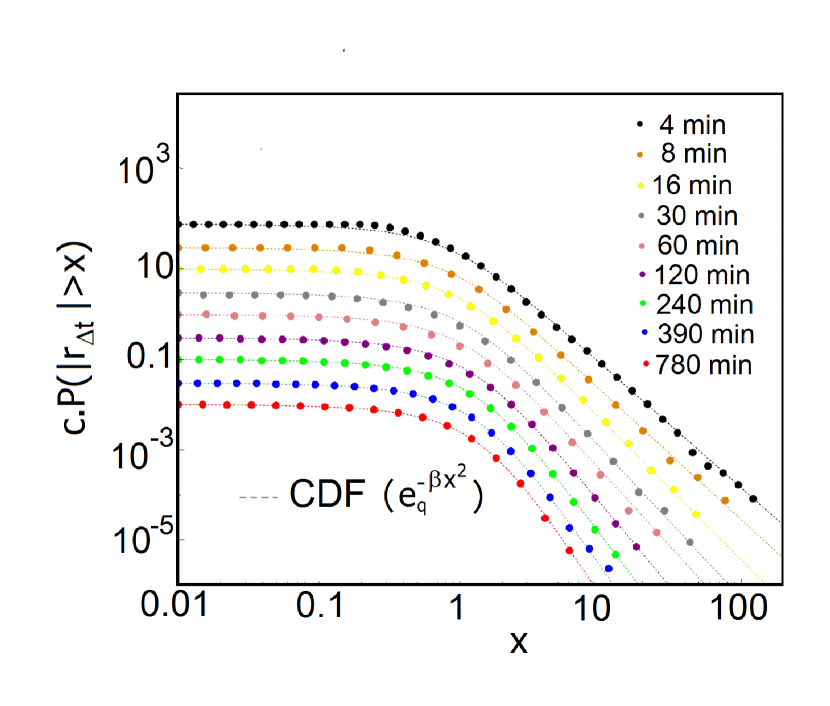
Figure 1: (Color online) Cumulative distributions of absolute normalized returns that correspond to different time scales $\Delta t$ for the 100 American companies with the highest market capitalization (points), and the fitted cumulative $q$-Gaussian distributions (lines). In order to better visualize the results, each $q$-Gaussian CDF and the respective experimental data have been multiplied by a positive factor, $c\neq 1$.

The asymptotic behavior of such normalized returns has been observed to follow an asymptotical power-law-like dependence of the type $CDF(x)\sim 1/x^{\alpha}$ ($\alpha>0$). This is but one of the arguments that make $q$-Gaussian distributions attractive to describe them; indeed $q$-Gaussian asymptotically ($x\gg 1$) develop a power-law form $G_{q}(x)\sim x^{2/1-q}$.

First, we analytically obtain the CDF of a $q$-Gaussian probability distribution function (pdf), with $\mu=0$ and re-normalized temperature $\beta^{-1}$, as

$$P(\left|r_{\Delta t}\right|>x)=1-2A(q,\beta)\,\,x\,\,_{2}F_{1}\left(\alpha,\delta;\gamma,\tau\right),$$ (6)

where $\alpha=1/2$, $\delta=1/(q-1)$, $\gamma=3/2$, $\tau=\beta\left(1-q\right)x^{2}$ and where ${}_{2}F_{1}\left(\alpha,\delta;\gamma,\tau\right)$ is the hypergeometric function. Eq. (6) provides a $q$-dependent asymptotical ($x\gg 1$) behavior of the type $\sim x^{(q-3)/(q-1)}$, that fits the $\alpha$-dependent asymptotical behavior of absolute normalized returns, and provides the $q$-Gaussian index through the relation:

$$q=\frac{3+\alpha}{1+\alpha}.$$ (7)

Even in the case that empirical data of a particular time scale did not attain the asymptotical behavior yet, we observe that cumulative distributions are also properly fitted by the CDF of a $q$-Gaussian pdf (6). We obtain the value of $\beta$ associated to the index $q$ that corresponds to each time scale $\Delta t$, by a least squares fitting technique. Our $q$ versus $\Delta t$ results (see table 1), are in a quite satisfactory agreement with [29].

Table 1: Time scales of absolute normalized returns, and the $(q,\beta)$ values of their respective estimated CDFs.

$\Delta t$	$q$	$\beta$
4	1.53	1.78
8	1.52	1.67
16	1.48	1.52
30	1.46	1.42
60	1.45	1.33
120	1.42	1.25
240	1.39	1.14
390	1.37	1.10
780	1.35	1.03

The fitted CDF are represented, for all time scales, in fig. 1, together with the experimental data provided in [29]. The convergence of the CDF exhibits that, as $\Delta t$ increases, the value of $q$ decreases. Hypothetical final convergence to a Gaussian ($q\to 1$) appears to be abrupt (see fig. 2).

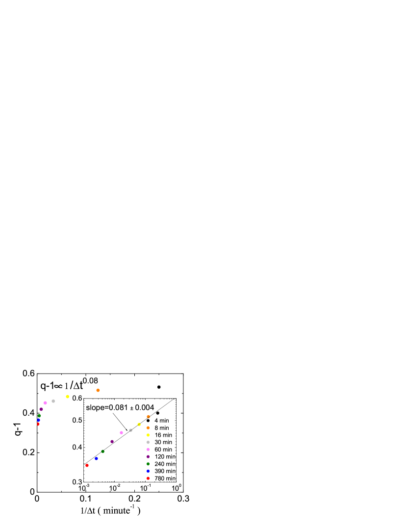
Figure 2: (Color on line) Dependence, versus temporal scale $\Delta t$, of nonextensive index $q$, for the estimated $q$-Gaussian pdfs of normalized absolute returns. Inset: Log-log representation shows a power-law dependence of the type $q-1\propto\Delta t^{-\tau}$, with $\tau=0.081\pm 0.004$.

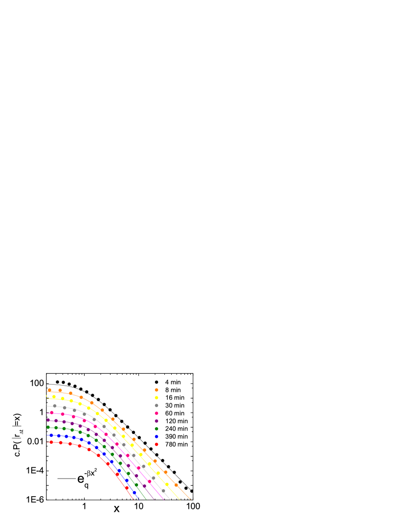
Figure 3: (Color on line) Log-log representation of the probability density distributions of absolute normalized returns for different time scales $\Delta t$. Points have been obtained by numerical derivation of cumulative values. Lines represent the $q$-Gaussian pdfs that lead to the fitted CDFs in fig.1. In order to better visualize the results, each $q$-Gaussian and the respective numerically estimated values, are multiplied by a positive factor $c\neq 1$.

Figure 4: Log-linear representation of the probability density distribution of absolute normalized returns, for time scale $\Delta t=4$. Points have been obtained by numerical derivation of cumulative values. Line represent the $q$-Gaussian pdf that leads to the corresponding CDF in fig.1, i.e., $q=1.53$ and $\beta=1.78$.

Fig. 3 and fig. 4 exhibit the good agreement with the $q$-Gaussian pdfs that lead to eq. (6), with respect to the derivatives of the experimental cumulative distributions.

Figure 5: Log-log representation of the re-normalized inverse temperature $\beta$ versus temporal scale $\Delta t$, for the estimated $q$-Gaussian pdfs of normalized absolute returns. A power-law dependence of the type $\beta^{-1}\propto\Delta t^{-\gamma}$ is observed, with $\gamma=0.106\pm 0.002$.

Figure 6: Log-log representation of the re-normalized inverse temperature $\beta$ versus $q-1$, for the estimated $q$-Gaussian pdfs of normalized absolute returns. A power-law dependence of the type $\beta^{-1}\propto(q-1)^{-\delta}$ is observed, with $\delta=1.29\pm 0.07$.

We have also observed that simple relations exist between the quantities $(q,\beta)$ involved for each time scale $\Delta t$. A power-law dependence is observed for both $q$ and $\beta$ as a function of time scale $\Delta t$, the exponents being $\tau=0.081\pm 0.004$ (fig. 2) and $\gamma=0.106\pm 0.002$ (fig. 5). Fig. 6 shows in fact that the re-normalized temperature $\beta^{-1}$ is not a free value, but it also exhibits a power-law dependence versus $q$, mainly $\beta^{-1}=(q-1)^{-\delta}$, with $\delta=1.29\pm 0.07$.

Summarizing, our results show that $q$-statistics describes complex systems that emerge in the analysis of the present particular financial data. Similar results have been previously obtained [16, 18, 29]. But, undoubtedly, the novelty of the present results is that we have also exhibited that both parameters $(q,\beta)$ of the nonextensive scenario are specific values that are fixed by $\Delta t$. Such a behavior is analogous to the behavior of a variety of other systems that are properly described by $q$-statistics, for example scale-free $d$-dimensional geographically-located networks [30], quark-gluon soup in high-energy particle collisions [31], LHC/CERN and RHIC/Brookhaven experiments [32] and anomalous diffusion in confined granular media [33]. Another simple and paradigmatic example is the logistic map where, as a reminiscence of this type of behavior, the $q$-generalized Lyapunov exponent depends on the value of $q$ that characterizes the sensitivity to initial conditions at the edge of chaos [34, 35]. This frequent feature comes from the fact that $q$-statistics typically emerges at critical-like regimes and appears to be deeply related to an hierarchical occupation of phase space.

We are grateful to professors J. Kwapień and S. Drożdż for sharing with us their empirical cumulative distribution data. One of us (G. R.) is grateful to professor C. Tsallis for is fruitful suggestions. One of us (G. R.) also acknowledges the warm hospitality at the CBPF (Brazil) and the partial financial support by the John Templeton Foundation (USA).

References

- [1] R. N. Mantegna and H. E. Stanley, An introduction to Econophysics: Correlations and Complexity in Finance (Cambridge University Press, Cambridge, 2000).
- [2] H. Takayasu H. (ed.) Empirical Science of Finantial Fluctuations: The Advent of Econophysics (Springer, Berlin, 2002).
- [3] A. Bunde, H. J. Schellnhuber and J. Kropp, The Science of Disasters: Climate Disruptions, Hearth Attacks and Market Crashes (Springer, Berlin, 2002).
- [4] L. Bachelier, Ann. Sci. École Norm. Suppl. 3, 21 (1900).
- [5] B. B. Mandelbrot, J. Business 36, 294 (1962).
- [6] A. Pagan, J. Empirical Finance 3, 15 (1996).
- [7] X. Gabaix, P. Gopikrishnan, V. Plerou and H. E. Stanley, Nature 423, 267 (2003).
- [8] P. Gopikrishnan, M. Meyer, L. A. N. Amaral, and H. E. Stanley, Eur. Phys. J. B 3, 138 (1998).
- [9] P. Gopikrishnan, V. Plerou, L. A. N. Amaral, M. Meyer and H. E. Stanley, Phys. Rev. E 60, 5305 (1999).
- [10] M. Denys, T. Gubiec, M. Jagielski, R. Kutner, and H. E. Stanley, Phys. Rev. E 94, 042305 (2016).
- [11] P. Oświecimka, J. Kwapień and S. Drożoż, Physica A 347, 626 (2005).
- [12] J. Kwapień, P. Oświecimka and S. Drożoż, Physica A 350, 466 (2005).
- [13] B. B. Mandelbrot, Fractals and Scaling in Finance (Springer, Berlin, 1997).
- [14] C. Tsallis, J. Stat. Phys. 52, 479 (1988).
- [15] C. Tsallis, Introduction to Nonextensive Statistical Mechanics – Approaching a Complex World (Springer, New York, 2009).
- [16] C. Tsallis, C. Anteneodo, L. Borland and R. Osorio, Physica A 324, 89 (2003).
- [17] F. Michael and M. D. Johnson, Physica A 320, 525 (2003).
- [18] R. Rak, S. Drożdż and J. Kwapień, Physica A 374, 315 (2007).
- [19] S. Drożdż, M. Forczek, J. Kwapień, P. Oświecimka and R. Rak, Physica A 383, 59 (2007).
- [20] J. Ludescher, C. Tsallis and A. Bunde, Eur. Phys. Lett. 95, 68002 (2011).
- [21] C. Tsallis, Chaos, Solitons and Fractals 88, 254 (2016).
- [22] C. Tsallis, S. V. F. Levy, A. M. C. Souza and R. Maynard, Phys. Rev. Lett. 75, 3589 (1995).
- [23] C. Tsallis, R.S. Mendes and A. R. Plastino, Physica A 261, 534 (1998).
- [24] C. Tsallis, A. R. Plastino and R. F. Alvarez-Estrada, J. Math. Phys. 50, 043303 (2009).
- [25] D. Prato and C. Tsallis, Phys. Rev. E 60, 2398 (1999).
- [26] L.G., Moyano, C. Tsallis and M. Gell-Mann, Europhys Lett 73, 813 (2006).
- [27] S. Umarov, C. Tsallis and S. Steinberg, Milan J. Math. 76, 307 (2008).
- [28] S. Umarov and C. Tsallis, J. Phys. A: Math. Theor. 49, 415204(2016).
- [29] J. Kwapień and S. Drożdż, Physics Report 515, 115 (2012).
- [30] S. G. A. Brito, L. R. da Silva and C. Tsallis, Nature - Scientific Reports 6, 27992 (2016).
- [31] D. B. Walton and Rafelshi J., Phys Rev. Lett. 84, 31 (2000).
- [32] V. Khachatryan et al., Phys. Rev. Lett. 105, 022002 (2010).
- [33] G. Combe, V. Richefeu, M. Stasiak and A. P. F. Atman, Phys Rev. Lett. 115, 238301 (2016).
- [34] M. L. Lyra and C. Tsallis, Phys. Rev. Lett 80, 53 (1998).
- [35] F. Baldovin and A. Robledo, Phys. Rev. E 69, 045202(R) (2004).