Comprehensive classification for Bose-Fermi mixtures

Abstract

We present analytical studies of a boson-fermion mixture at zero temperature with spin-polarized fermions. Using the Thomas-Fermi approximation for bosons and the local-density approximation for fermions, we find a large variety of different density shapes. In the case of continuous density, we obtain analytic conditions for each configuration for attractive as well as repulsive boson-fermion interaction. Furthermore, we analytically show that all the scenarios we describe are minima of the grand-canonical energy functional. Finally, we provide a full classification of all possible ground states in the interpenetrative regime. Our results also apply to binary mixtures of bosons.

1 Introduction

Since the experimental observation of Bose-Einstein condensation [1, 2], interest was also oriented toward the study of ultracold fermions and mixtures of bosons and fermions. The theoretical study of the density profiles of trapped boson-fermion mixtures was done, however, mainly numerically, only carried out for certain parameter ranges, and stability considerations lacked completeness. In this paper we provide a comprehensive classification of all continuous ground-state profiles of a spin-polarized boson-fermion mixture, we will derive analytic conditions for each scenario, and rigorously show stability.

1.1 The richness of Bose-Fermi mixtures

Originally, interest in ultracold fermions was, among other reasons, spurred by the possible observation of the famous transition to the Bardeen-Cooper-Schrieffer state. Quantum degeneracy for fermionic systems, however, was hard to achieve as the Pauli exclusion principle forbids $s$-wave scattering in a spin-polarized sample and $p$-wave interaction is strongly suppressed at low temperatures [3]. Therefore, a fermionic gas cannot be cooled evaporatively in a magnetic trap. This problem was circumvented by preparing the system in two spin states [4] or by employing boson-fermion mixtures, where the Bose-Einstein condensate is cooled evaporatively and then used as a sympathetic coolant for the fermionic species [5, 6, 7]. When boson-fermion mixtures with attractive interaction between the components were studied [8], a collapse of the system was observed [9] whenever the number of fermions exceeded a certain threshold as predicted by Ref. [10]. A Feshbach resonance enabled [11, 12] to tune the boson-fermion interaction from the collapse at attractive values via regimes where the densities interpenetrate to strong repulsion, where the system tends to demix. While the onset of superfluidity in a pure Fermi mixture of two spin states was proved in 2005 by the observation of quantized vortices [13], it was not until 2014 that the simultaneous superfluidity of a boson-fermion mixture was observed at unitarity [14].
A lot of effort has also been devoted to boson-fermion mixtures on the theoretical side to analyze the phase diagram. Describing the bosons by the Gross-Pitaevskii equation and the fermions within the local-density approximation, the collapse in attractive mixtures was studied numerically [10, 15, 16, 17, 18, 19], semi-analytically by a variational Gauss ansatz [20, 21], or in the Thomas-Fermi approximation [22]. Scaling laws to determine the boundaries in parameter space between collapse, mixing, and phase separation were obtained as functions of the chemical potential. Their dependence on the particle numbers, however, could only be established numerically or by rough estimates.
Repulsive interaction leads to a large variety of stable density configurations in the mixed regime, some of which were found numerically in Refs. [23, 24, 25, 26]. In addition, many interesting cases in the phase-separated region, e.g. mirror-symmetry breaking or the ‘boson burger’ in an anisotropic trap were investigated in Ref. [23]. The discussion was complemented by further ‘exotic’ configurations found at higher energies [25]. A thorough stability consideration was made for the homogeneous case [27] but has not been generalized to trapped systems yet. Finally, the influence of finite temperature [28, 29] and beyond mean-field effects [30, 31, 32, 33] have also been investigated.

1.2 Methodology

In this paper we consider a mixture of a Bose-Einstein condensate with fermions, which are either spin polarized or at unitarity. We provide a comprehensive classification of possible ground states in the regime where the densities are continuous. Configurations with discontinuities, for example when phase separation occurs, will only be discussed briefly. In our classification of density shapes we group the large variety of different configurations with respect to characteristic features, e.g. the number of maxima in the densities or which species encloses the other, similarly to what has been done for a binary mixture of Bose-Einstein condensates in [34] and [35]. A summary of our results can be found in Fig. 1 for repulsive interaction and in Fig. 2 for attractive interaction.

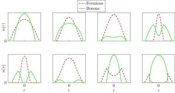
Figure 1: Possible density profiles within our classification scheme for repulsive interaction. Analytical conditions for every configuration and their detailed derivation will be presented in subsequent sections. The parameters involved are: The chemical potentials, the confinement for each species, and the interaction strength among the particles.

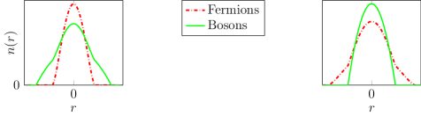
Figure 2: Possible density profiles within our classification scheme for attractive interaction.

Working in the Thomas-Fermi approximation for bosons [36] and the local-density approximation for fermions [37], the equations for the densities could in principle be solved analytically by means of Cardano’s formula. It is, however, much more instructive to deduce simple but rigorous algebraic conditions which determine the qualitative density shapes by understanding the behavior of the equations for a given set of parameters. The discussion will be supplemented with a thorough stability consideration. Indeed, we will rigorously show stability for all the configurations we find. The conditions contain the chemical potentials $\mu_{\mathrm{F}}$ and $\mu_{\mathrm{B}}$ as parameters rather than the particle numbers $N_{\mathrm{F}}$ and $N_{\mathrm{B}}$. We will not be able to provide an analytic relation between $N$ and $\mu$ due to the nonlinearity of the equations. For that, one still has to resort to numerical methods. Moreover, it should be noted that conditions are stated using $>,<$ instead of $\geq,\leq$ since the subset of parameters where the real equalities hold has zero measure.
Finally, let us comment upon the reliability of our model. While the local-density approximation precisely describes the fermionic density even for a small number of particles, the Thomas-Fermi approximation is only expected to provide accurate results when the bosonic density behaves smoothly and the particle number is not too small. In the vicinity of sharp edges, which e.g. occur in the case of phase separation or at the surface of the cloud, the density will be smoothed out as predicted by the Gross-Pitaevskii equation [38], but the Thomas-Fermi approximation is still expected to provide qualitatively correct results.
Furthermore, it should be emphasized that by a certain choice of parameters our model also reproduces all the possible density configurations for Bose-Bose mixtures.

1.3 Overview

The paper is structured as follows. In Sec. 2 we minimize the grand-cannonical energy functional and obtain nonlinear equations from which the density distributions follow. The structure of the equations allows several solution branches. In Sec. 3 we derive stability conditions to determine which of those are stable and obtain conditions for the number of solutions. We then turn to the shape of the solutions. By using geometric arguments we first study the fermionic density profiles in Sec. 4. Using the results of A, we also establish the bosonic profiles and provide a full classification of all possible ground-state density configurations for the boson-fermion mixture in Sec. 5.

2 Minima of the grand-canonical energy

In this section we compute the first and second functional derivative of the energy functional and obtain equations for the density shapes as well as conditions for stability.

2.1 Energy functional

We start our consideration with the mean-field energy functional

$$E[n_{\mathrm{B}},n_{\mathrm{F}}]=\int\mathrm{d}^{3}\mathbf{r}\bigg{(}\frac{1}{2}g_{\mathrm{B}}n^{2}_{\mathrm{B}}(\mathbf{r})+V_{\mathrm{B}}(\mathbf{r})n_{\mathrm{B}}(\mathbf{r}) +\frac{1}{\gamma+1}\kappa n_{\mathrm{F}}(\mathbf{r})^{\gamma+1}+V_{\mathrm{F}}(\mathbf{r})n_{\mathrm{F}}(\mathbf{r})$$

$$+g_{\mathrm{BF}}n_{\mathrm{F}}(\mathbf{r})n_{\mathrm{B}}(\mathbf{r})\bigg{)}\;,$$ (2.1)

of a boson-fermion mixture in the Thomas-Fermi approximation for bosons and in the local-density approximation for fermions. We have introduced the real parameter $\gamma\in(0,1)$ as a generalization. If $\gamma=2/3$, we obtain the energy functional of a spin polarized boson-fermion mixture at quantum degeneracy with $\kappa=\frac{\hbar^{2}}{2m_{\mathrm{F}}}(6\pi^{2})^{2/3}$. Likewise, for a mixture of superfluid bosons and fermions at unitarity $\kappa=\xi\frac{\hbar^{2}}{2m_{\mathrm{F}}}(3\pi^{2})^{2/3}$ [39], where $\xi$ is a dimensionless renormalization factor. Conversely, $\gamma\rightarrow 1$ describes a boson-boson mixture where $\kappa$ is the particle-particle interaction parameter of one bosonic species. The fermionic and bosonic potentials, $V_{\mathrm{B}}$ and $V_{\mathrm{F}}$, can be very general. The minimal requirement is that $V_{\mathrm{F}}=\alpha_{\mathrm{F}}V$ and $V_{\mathrm{B}}=\alpha_{\mathrm{B}}V$, where $\alpha_{\mathrm{B}},\alpha_{\mathrm{F}}>0$ are constant factors and $V$ is monotonic in the sense that for any given direction $\mathbf{d}$ the function

$$\tilde{V}(r)=V(r\mathbf{d})$$ (2.2)

is monotonic for $r>0$. Additionally, we choose $V(0)=0$ at $\mathbf{r}=0$ and $V$ to be continuous.
$n_{\mathrm{B}}$ and $n_{\mathrm{F}}$ are the bosonic and fermionic particle densities, $g_{\mathrm{B}}$ the bosonic particle-particle interaction parameter, and $g_{\mathrm{BF}}$ accounts for the interspecies interaction.
To keep notation simple, we will omit the spatial coordinate $\mathbf{r}$ throughout the whole paper.

2.2 First derivative of the energy functional

We will now calculate the first functional derivative of Eq. (2.1) in order to obtain equations for the density configurations. Assuming chemical equilibrium with particle reservoirs, the state of the system minimizes the grand-canonical energy

$$K[n_{\mathrm{B}},n_{\mathrm{F}}]=\int\mathrm{d}^{3}\mathbf{r}\,\mathcal{K}=\int\mathrm{d}^{3}\mathbf{r}\,\left(\mathcal{E}-\mu_{\mathrm{B}}n_{\mathrm{B}}-\mu_{\mathrm{F}}n_{\mathrm{F}}\right)$$ (2.3)

at zero temperature, where the energy density $\mathcal{E}$ is given by the integrand of Eq. (2.1). In order to perform the minimization, we first split the integral into three parts $\Omega_{\mathrm{B}}=\left\{\mathbf{r}:n_{\mathrm{B}}\neq 0,n_{\mathrm{F}}=0\right\}$, $\Omega_{\mathrm{F}}=\left\{\mathbf{r}:n_{\mathrm{B}}=0,n_{\mathrm{F}}\neq 0\right\}$, and $\Omega_{\mathrm{BF}}=\left\{\mathbf{r}:n_{\mathrm{B}}\neq 0,n_{\mathrm{F}}\neq 0\right\}$ to characterize regions where either the bosonic or fermionic density equals zero or both species coexist. Thus, the first variation of Eq. (2.3) reads

$$\delta K[n_{\mathrm{B}},n_{\mathrm{F}}] =\delta K_{\Omega_{\mathrm{BF}}}+\delta K_{\Omega_{\mathrm{F}}}+\delta K_{\Omega_{\mathrm{B}}}$$

$$=\int_{\Omega_{\mathrm{BF}}}\mathrm{d}^{3}\mathbf{r}\left(\frac{\partial\mathcal{K}}{\partial n_{\mathrm{B}}}\delta n_{\mathrm{B}}+\frac{\partial\mathcal{K}}{\partial n_{\mathrm{F}}}\delta n_{\mathrm{F}}\right)$$

$$+\int_{\Omega_{\mathrm{F}}}\mathrm{d}^{3}\mathbf{r}\left.\left(\frac{\partial\mathcal{K}}{\partial n_{\mathrm{B}}}\delta n_{\mathrm{B}}+\frac{\partial\mathcal{K}}{\partial n_{\mathrm{F}}}\delta n_{\mathrm{F}}\right)\right|_{n_{\mathrm{B}}=0}$$

$$+\int_{\Omega_{\mathrm{B}}}\mathrm{d}^{3}\mathbf{r}\left.\left(\frac{\partial\mathcal{K}}{\partial n_{\mathrm{B}}}\delta n_{\mathrm{B}}+\frac{\partial\mathcal{K}}{\partial n_{\mathrm{F}}}\delta n_{\mathrm{F}}\right)\right|_{n_{\mathrm{F}}=0}\;.$$ (2.4)

Using Eq. (2.1), we obtain the relations

$$\delta K_{\Omega_{\mathrm{BF}}} =\int_{\Omega_{\mathrm{BF}}} \mathrm{d}^{3}\mathbf{r}\left(g_{\mathrm{B}}n_{\mathrm{B}}+V_{\mathrm{B}}+g_{\mathrm{BF}}n_{\mathrm{F}}-\mu_{\mathrm{B}}\right)\delta n_{\mathrm{B}}$$

$$+\int_{\Omega_{\mathrm{BF}}} \mathrm{d}^{3}\mathbf{r}\left(\kappa n_{\mathrm{F}}^{\gamma}+V_{\mathrm{F}}+g_{\mathrm{BF}}n_{\mathrm{B}}-\mu_{\mathrm{F}}\right)\delta n_{\mathrm{F}}\;,$$ (2.5)

$$\delta K_{\Omega_{\mathrm{F}}} =\int_{\Omega_{\mathrm{F}}} \mathrm{d}^{3}\mathbf{r}\left(V_{\mathrm{B}}+g_{\mathrm{BF}}n_{\mathrm{F}}-\mu_{\mathrm{B}}\right)\delta n_{\mathrm{B}}+\int_{\Omega_{\mathrm{F}}}\mathrm{d}^{3}\mathbf{r}\left(\kappa n_{\mathrm{F}}^{\gamma}+V_{\mathrm{F}}-\mu_{\mathrm{F}}\right)\delta n_{\mathrm{F}}\;,$$ (2.6)

$$\delta K_{\Omega_{\mathrm{B}}} =\int_{\Omega_{\mathrm{B}}} \mathrm{d}^{3}\mathbf{r}\left(g_{\mathrm{B}}n_{\mathrm{B}}+V_{\mathrm{B}}-\mu_{\mathrm{B}}\right)\delta n_{\mathrm{B}}+\int_{\Omega_{\mathrm{B}}}\mathrm{d}^{3}\mathbf{r}\left(V_{\mathrm{F}}+g_{\mathrm{BF}}n_{\mathrm{B}}-\mu_{\mathrm{F}}\right)\delta n_{\mathrm{F}}\;.$$ (2.7)

We now search for $n_{\mathrm{B}}$ and $n_{\mathrm{F}}$ such that

$$\delta K[n_{\mathrm{B}},n_{\mathrm{F}}]\geq 0$$ (2.8)

for every infinitesimal $\delta n_{\mathrm{B}}$, $\delta n_{\mathrm{F}}$. We note that $\delta n(\mathbf{r}_{1})$ is independent of $\delta n(\mathbf{r}_{2})$ for $\mathbf{r}_{1}\neq\mathbf{r}_{2}$, so Eq. (2.8) has to be fulfilled in every region $\Omega_{\mathrm{F}}$, $\Omega_{\mathrm{B}}$, and $\Omega_{\mathrm{BF}}$ independently.
Let us disregard for the moment the first term in Eq. (2.6) and the second in Eq. (2.7). We will turn to them in Sec. 2.3. Choosing

$$\mu_{\mathrm{B}} =V_{\mathrm{B}}+g_{\mathrm{B}}n_{\mathrm{B}}+g_{\mathrm{BF}}n_{\mathrm{F}} \mathbf{r}\in\Omega_{\mathrm{BF}}\;,$$ (2.9)

$$\mu_{\mathrm{F}} =V_{\mathrm{F}}+\kappa n_{\mathrm{F}}^{\gamma}+g_{\mathrm{BF}}n_{\mathrm{B}} \mathbf{r}\in\Omega_{\mathrm{BF}}\;,$$ (2.10)

$$\mu_{\mathrm{B}} =V_{\mathrm{B}}+g_{\mathrm{B}}n_{\mathrm{B}} \mathbf{r}\in\Omega_{\mathrm{B}}\;,$$ (2.11)

$$\mu_{\mathrm{F}} =V_{\mathrm{F}}+\kappa n_{\mathrm{F}}^{\gamma} \mathbf{r}\in\Omega_{\mathrm{F}}\,,$$ (2.12)

then leads to

$$\delta K[n_{\mathrm{B}},n_{\mathrm{F}}]=0\,,$$ (2.13)

so that the solutions of these equations make Eq. (2.3) stationary.

2.3 Second derivative of the energy functional

In order to be a minimum, the second variation has to be greater than zero, which yields the expressions

$$0< \int_{\Omega_{\mathrm{F}}} \mathrm{d}^{3}\mathbf{r}\,\gamma\kappa\,n_{\mathrm{F}}^{\gamma-1}\,(\delta n_{\mathrm{F}})^{2}\;,$$ (2.14)

$$0< \int_{\Omega_{\mathrm{B}}} \mathrm{d}^{3}\mathbf{r}\,g_{\mathrm{B}}\,(\delta n_{\mathrm{B}})^{2}\;,$$ (2.15)

$$0< \int_{\Omega_{\mathrm{BF}}} \mathrm{d}^{3}\mathbf{r}\begin{pmatrix}\delta n_{\mathrm{B}}&\delta n_{\mathrm{F}}\end{pmatrix}\begin{pmatrix}g_{\mathrm{B}}&g_{\mathrm{BF}}\\ g_{\mathrm{BF}}&\gamma\kappa n_{\mathrm{F}}^{\gamma-1}\end{pmatrix}\begin{pmatrix}\delta n_{\mathrm{B}}\\ \delta n_{\mathrm{F}}\end{pmatrix}\;.$$ (2.16)

Note that Eq. (2.14) is always satisfied as $\kappa$ and $(\delta n_{\mathrm{F}})^{2}$ are always greater than zero. From Eq. (2.15) we deduce that

$$g_{\mathrm{B}}>0$$ (2.17)

must hold true since $(\delta n_{\mathrm{B}})^{2}>0$. Therefore, stable configurations only exist for repulsive interaction among the bosons. The expression Eq. (2.16) is fulfilled for every possible infinitesimal variation of the densities exactly if the matrix is positive definite, which is true exactly if the leading principal minors are greater than zero, since the matrix is symmetric. This again provides us with $g_{\mathrm{B}}>0$ together with the condition

$$n_{\mathrm{F}}<\left(\frac{\gamma g_{\mathrm{B}}\kappa}{g_{\mathrm{BF}}^{2}}\right)^{\frac{1}{1-\gamma}}\;\;\;\;\;\;\;\;\;\;\;\;\;\forall\mathbf{r}\in\Omega_{\mathrm{BF}}\,,$$ (2.18)

which imposes a constraint on the fermionic density.
We now turn to the first contribution in Eq. (2.6). The bosonic density is zero in $\Omega_{\mathrm{F}}$, therefore only $\delta n_{\mathrm{B}}\geq 0$ for all $\mathbf{r}\in\Omega_{\mathrm{F}}$ are valid density variations, so that the bosonic density corresponds to a physical density which is larger than zero. The same applies to the fermionic density variation for the second term in Eq. (2.7). Because of that, Eq. (2.8) is satisfied by the additional requirement

$$V_{\mathrm{B}} +g_{\mathrm{BF}}n_{\mathrm{F}}-\mu_{\mathrm{B}}\geq 0 \forall\mathbf{r}\in\Omega_{\mathrm{F}}$$ (2.19)

$$V_{\mathrm{F}} +g_{\mathrm{BF}}n_{\mathrm{B}}-\mu_{\mathrm{F}}\geq 0 \forall\mathbf{r}\in\Omega_{\mathrm{B}}\;.$$ (2.20)

Hence, there exist density variations where Eq. (2.8) is true with the $>$-sign. In summary we have shown that the solutions of Eq. (2.9)-(2.12), (2.17), (2.18), (2.19) and Eq. (2.20) correspond to a minimum of the grand-canonical energy functional, which, however, due to Eq. (2.19) and Eq. (2.20) do not necessarily make Eq. (2.3) stationary.
It is easy to recognize that the solutions correspond to a minimum if and only if these conditions hold true because if only one is violated, one can always choose $\delta n_{\mathrm{B}}$, $\delta n_{\mathrm{F}}$ such that Eq. (2.8) is violated, too and therefore the densities do not correspond to a minimum anymore.

We conclude this section by noting that the stability considerations made above are valid for any topology of $\Omega_{\mathrm{BF}}$, $\Omega_{\mathrm{B}}$, and $\Omega_{\mathrm{F}}$. In principle, one can think of three classes of solutions:
The first are configurations with $\Omega_{\mathrm{BF}}$ being the empty set, i.e. the two species do not interpenetrate each other. In this case we have to solve Eq. (2.11) on $\Omega_{\mathrm{B}}$ and Eq. (2.12) on $\Omega_{\mathrm{F}}$, which in general lead to discontinuities in the densities. One can also think of a second class of solutions where $\Omega_{\mathrm{BF}}$ exists but there still is at least one discontinuity. The densities calculated for these two classes, however, will only be local minima of $K$ when (2.19) and Eq. (2.20) are satisfied, that is, only for certain parameter ranges and topologies of the pure regions. We will refer to every stable, discontinuous configuration with a coexisting region as ‘partially phase separated’ and as ‘fully phase separated’ if there is no such region. In C it is shown that in the case of $g_{\mathrm{BF}}<0$ phase separation cannot occur. A further discussion of this interesting phenomenon, however, is not within the main scope of this paper.
We want to focus on the third class of solutions, that is, configurations with continuous densities. These are constructed as follows. For a given set of parameters we first solve Eq. (2.9) and (2.10). If existent, $\Omega_{\mathrm{BF}}$ is given by the region where both densities are larger than zero. We also obtain the boundaries of this region, which is where one of the densities first reaches zero. We then use Eq. (2.11) and (2.12), respectively, to calculate the densities in the regions where only one particle species exists. Finally, we have to disregard all solutions which do not agree with Eq. (2.18). As it will turn out, this condition can be used to select the stable solution branch out of all possible solutions. We will furthermore show in B that every density configuration constructed in this manner is a local minimum of $K$, that is, the conditions (2.19) and (2.20) will be automatically satisfied.

3 Existence and number of real solutions

In the previous section we have derived conditions from the energy functional, which allow us to calculate density distributions for a given set of parameters. In this section we will examine the nonlinear equations for the density configurations, derive a simple criterion for the stability of a solution branch, and determine conditions for the number of possible solutions.

3.1 Selection of the stable solution branch

In order to distinguish stable solutions of Eq. (2.9) and Eq. (2.10) from those which are unphysical, we will now elucidate how to use the constraint Eq. (2.18) on the fermionic density.
By substituting Eq. (2.9) and (2.10) into each other, the two equations can be decoupled as follows:

$$n_{\mathrm{F}}^{\gamma}=\frac{1}{\kappa}\left(\mu_{\mathrm{F}}-\frac{g_{\mathrm{BF}}}{g_{\mathrm{B}}}\mu_{\mathrm{B}}\right)+\frac{1}{\kappa}\left(\frac{g_{\mathrm{BF}}}{g_{\mathrm{B}}}\alpha_{\mathrm{B}}-\alpha_{\mathrm{F}}\right)V+\frac{g_{\mathrm{BF}}^{2}}{g_{\mathrm{B}}\kappa}n_{\mathrm{F}}$$ (3.21)

$$\frac{\kappa^{\frac{1}{\gamma}}}{g_{\mathrm{BF}}}\left(\mu_{\mathrm{B}}-V_{\mathrm{B}}\right)-\frac{\kappa^{\frac{1}{\gamma}}g_{\mathrm{B}}}{g_{\mathrm{BF}}}n_{\mathrm{B}}=\left(\mu_{\mathrm{F}}-V_{\mathrm{F}}-g_{\mathrm{BF}}n_{\mathrm{B}}\right)^{\frac{1}{\gamma}}.$$ (3.22)

As the equations are nonlinear in the densities, we expect several solution branches for a given set of parameters. Obviously, not every solution is positive or even real, so we do not necessarily find physical solutions in every case. By means of geometric arguments we will demonstrate that there are always none, one, or two real solutions to both Eq. (3.21) and (3.22). Furthermore, we will derive criteria for deciding which corresponds to a minimum of Eq. (2.1). To do this, we consider both sides of Eq. (3.21) as functions of $n_{\mathrm{F}}$. Then, for a given value of $\mathbf{r}$ there exists a real solution when the concave function $n_{\mathrm{F}}^{\gamma}$, corresponding to the left-hand side, intersects with the straight line, the right-hand side of the equation. This can be seen in Fig. 3.

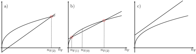
Figure 3: Geometric method to solve Eq. (3.21). Plot of the right-hand side (straight line) and the left-hand side (concave function) as a function of $n_{\mathrm{F}}$. The points where these two functions intersect correspond to the solutions of Eq. (3.21). There are three possible scenarios depending on the set of parameters: One solution: Fig. 3.a, two solutions: Fig. 3.b, and no solution: Fig. 3.c.

Since $\frac{g_{\mathrm{BF}}^{2}}{g_{\mathrm{B}}\kappa}>0$, the straight line always has positive slope and there are exactly three possible scenarios. There are either zero, one or two intersection points and therefore either no, one or two real solutions to Eq. (3.21). The same conclusion can be drawn for Eq. (3.22). Given a solution $n_{\mathrm{F}}$, it can be substituted in Eq. (2.9) yielding a real solution for $n_{\mathrm{B}}$ as well.
We now determine, which of those solutions are physically stable and which are not. To do this, we first turn to the situation where there are two intersection points, which we shall denote by $n_{\mathrm{F}{(1)}}$ and $n_{\mathrm{F}{(2)}}$. This situation is visualized in Fig. 3.b. The mean value theorem states that there always exists a $n_{\mathrm{F}{(0)}}\in\left(n_{\mathrm{F}{(1)}},n_{\mathrm{F}{(2)}}\right)$ such that the slope of the tangent to the concave function, given by the first derivative $\mathrm{d}\left(n_{\mathrm{F}}^{\gamma}\right)/\mathrm{d}n_{\mathrm{F}}$ at $n_{\mathrm{F}}=n_{\mathrm{F}(0)}$, equals the slope of the straight line. This leads to the relation

$$\gamma\,n_{\mathrm{F}(0)}^{\gamma-1} =\frac{g_{\mathrm{BF}}^{2}}{g_{\mathrm{B}}\kappa}$$ (3.23)

or, equivalently,

$$n_{\mathrm{F}(0)} =\left(\frac{\gamma g_{\mathrm{B}}\kappa}{g_{\mathrm{BF}}^{2}}\right)^{\frac{1}{1-\gamma}}\;.$$ (3.24)

Comparison with Eq. (2.18) then shows that $n_{\mathrm{F}(2)}>n_{\mathrm{F}(0)}$ is unstable. Similarly, in the case of one intersection point $n_{\mathrm{F}(2)}$ as depicted in Fig. 3.a we rewrite Eq. (3.21) as

$$0 =c+\frac{g_{\mathrm{BF}}^{2}}{g_{\mathrm{B}}\kappa}n_{\mathrm{F}(2)}-n_{\mathrm{F}(2)}^{\gamma}\;,$$ (3.25)

where $$c c<0$$ is the ordinate intersection of the straight line and therefore or, equivalently,

$$-c =\frac{g_{\mathrm{BF}}^{2}}{g_{\mathrm{B}}\kappa}n_{\mathrm{F}(2)}-n_{\mathrm{F}(2)}^{\gamma}>0\;,$$ (3.26)

which yields after rearranging

$$n_{\mathrm{F}(2)}>\left(\frac{g_{\mathrm{B}}\kappa}{g_{\mathrm{BF}}^{2}}\right)^{\frac{1}{1-\gamma}}>\left(\frac{\gamma g_{\mathrm{B}}\kappa}{g_{\mathrm{BF}}^{2}}\right)^{\frac{1}{1-\gamma}}\;.$$ (3.27)

Thus, $n_{\mathrm{F}(2)}$ is an unstable solution.
In summary, we have shown that if there exists exactly one solution branch, it is unstable. In the case of two solutions only the fermionic branch with the smaller value is stable. If there exist two fermionic solution branches, there are two bosonic as well because of relation Eq. (2.9). We now establish which bosonic branch belongs to the stable fermionic one. For this purpose, we denote again the different solutions by $n_{\mathrm{F}(1)}$, $n_{\mathrm{B}(1)}$ and $n_{\mathrm{F}(2)}$, $n_{\mathrm{B}(2)}$. When we substitute each solution into Eq. (2.9) and subtract the resulting expressions from each other, we arrive at

$$0=g_{\mathrm{B}}\left(n_{\mathrm{{B}(1)}}-n_{\mathrm{{B}(2)}}\right)+g_{\mathrm{BF}}\left(n_{\mathrm{{F}(1)}}-n_{\mathrm{{F}(2)}}\right)\;.$$ (3.28)

Let $n_{\mathrm{{F}(1)}}$ be the fermionic solution with the smaller value. For $g_{\mathrm{BF}}>0$ the second contribution in Eq. (3.28) is then smaller than zero. Hence, the first term is larger than zero and therefore $n_{\mathrm{{B}(1)}}>n_{\mathrm{{B}(2)}}$. Thus, the fermionic solution with the smaller value corresponds to the bosonic solution with the greater value and these solutions are stable. In contrast, for $g_{\mathrm{BF}}<0$ the smaller fermionic solution corresponds to the smaller bosonic one, which are the stable solutions in this case.

3.2 Conditions for the number of solutions

The next step is to derive conditions which determine the number of real solutions to Eq. (3.21) and (3.22). We start our analysis by introducing the following abbreviations in Eq. (3.21):

$$d=\frac{g_{\mathrm{BF}}^{2}}{g_{\mathrm{B}}\kappa}\;\;\;\;\text{and}\;\;\;\;c=\frac{1}{\kappa}\left(\mu_{\mathrm{F}}-\frac{g_{\mathrm{BF}}}{g_{\mathrm{B}}}\mu_{\mathrm{B}}\right)+\frac{1}{\kappa}\left(\frac{g_{\mathrm{BF}}}{g_{\mathrm{B}}}\alpha_{\mathrm{B}}-\alpha_{\mathrm{F}}\right)V\;,$$ (3.29)

which lead to

$$n_{\mathrm{F}}^{\gamma}=d\,n_{\mathrm{F}}+c\;,$$ (3.30)

and where it is important to note that $\gamma\in(0,1)$ and $d>0$.
As discussed above and seen from Fig. 3.a, for $c<0$ there is one positive solution.
Let us analyze what happens for $c>0$. We start our consideration by noting that the derivative of $n^{\gamma}$ with respect to $n$ is greater than zero for $n\in(0,\infty)$. Then it follows that for every $c>0$ there exists one $d_{0}>0$ such that the straight line $y=d_{0}\,n_{\mathrm{F}}+c$ is tangent to $y=n_{\mathrm{F}}^{\gamma}$ at $n_{\mathrm{F}}=n_{\mathrm{F}(0)}$ as can be seen in Fig. 4. Thus, we find

no real solution for $$d>d_{0}$$ (3.31)

and two positive solutions for $$d<d_{0}\;.$$ (3.32)

When we solve the system of equations

$$\gamma n_{\mathrm{F}(0)}^{\gamma-1} =d_{0}\;,$$ (3.33)

$$n_{\mathrm{F}(0)}^{\gamma} =d_{0}n_{\mathrm{F}(0)}+c\;,$$ (3.34)

we obtain the explicit expression

$$d_{0}=\gamma\left(\frac{1-\gamma}{c}\right)^{\frac{1-\gamma}{\gamma}}\;.$$ (3.35)

Finally, the combination of Eq. (3.35) with Eq. (3.31) and (3.32) leads after rearranging terms to the conditions

$$\left(\frac{\gamma}{d}\right)^{\frac{\gamma}{1-\gamma}}\left(1-\gamma\right)\; <\; c\quad\quad$$ for no real solution, (3.36)

$$\left(\frac{\gamma}{d}\right)^{\frac{\gamma}{1-\gamma}}\left(1-\gamma\right)\; >\; c>0\quad\quad$$ for two positive solutions, and (3.37)

$$c<0\quad\quad$$ for one positive solution. (3.38)

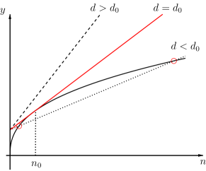
Figure 4: Visualization of Eq. (3.30). Plot of the left-hand side (concave function) and the right-hand side (straight line), which intersect at points that correspond to a solution. For every $c>0$ there exists a single straight line (solid line) with slope $d_{0}$ which is tangent to the concave function. If $d<d_{0}$, there are two solutions (dotted line) and if $d>d_{0}$, there is no solution (dashed line).

Substituting back the expressions for $d$ and $c$ according to Eq. (3.29), the three cases become

- no real solution if

$$\chi\left(1-\gamma\right)< \left(\mu_{\mathrm{F}}-\frac{g_{\mathrm{BF}}}{g_{\mathrm{B}}}\mu_{\mathrm{B}}\right)+\left(\frac{g_{\mathrm{BF}}}{g_{\mathrm{B}}}\alpha_{\mathrm{B}}-\alpha_{\mathrm{F}}\right)V\;,$$ (3.40)

- two solutions if

$$\chi\left(1-\gamma\right)> \left(\mu_{\mathrm{F}}-\frac{g_{\mathrm{BF}}}{g_{\mathrm{B}}}\mu_{\mathrm{B}}\right)+\left(\frac{g_{\mathrm{BF}}}{g_{\mathrm{B}}}\alpha_{\mathrm{B}}-\alpha_{\mathrm{F}}\right)V>0\;,$$ (3.41)

- one solution if

$$\left(\mu_{\mathrm{F}}-\frac{g_{\mathrm{BF}}}{g_{\mathrm{B}}}\mu_{\mathrm{B}}\right)+\left(\frac{g_{\mathrm{BF}}}{g_{\mathrm{B}}}\alpha_{\mathrm{B}}-\alpha_{\mathrm{F}}\right)V<0\;.$$ (3.42)

Here, we have defined

$$\chi:=\kappa\left(\frac{g_{\mathrm{B}}\kappa\gamma}{g^{2}_{\mathrm{BF}}}\right)^{\frac{\gamma}{1-\gamma}}$$ (3.43)

for convenience. These conditions also determine the possible solutions for the bosonic density, which follow from Eq. (3.22). This is because given any solution for the fermionic density, the bosonic density can be easily obtained from the linear relation Eq. (2.9). For example, if there are two fermionic branches, there will be two bosonic ones as well. The value of the bosonic solutions can, however, be negative, which does not correspond to a physical density. Therefore, their positivity needs to be explicitly checked. This will be done in A.

4 Qualitative shape of the fermionic solutions

At first sight these conditions may not seem very helpful. However, we will show that one can already make a full classification of the qualitative shape of the solutions to Eq. (3.21) from the conditions that we have derived in the previous sections. To this end, we will again make use of geometric arguments. Recall from Eq. (3.29) that $c$ depends on $V(\mathbf{r})$ and therefore on $\mathbf{r}$. Since $V$ is monotonic, an increase of $|\mathbf{r}|$ corresponds to a vertical shift of the straight line in Fig. 3. The line moves

upwards if $$\frac{g_{\mathrm{BF}}}{g_{\mathrm{B}}}\alpha_{\mathrm{B}}-\alpha_{\mathrm{F}}>0\;\;\text{ and}$$ (4.44)

downwards if $$\frac{g_{\mathrm{BF}}}{g_{\mathrm{B}}}\alpha_{\mathrm{B}}-\alpha_{\mathrm{F}}<0\;.$$ (4.45)

At the origin $V(\mathbf{r})=0$ by definition and therefore

$$c=\frac{1}{\kappa}\left(\mu_{\mathrm{F}}-\frac{g_{\mathrm{BF}}}{g_{\mathrm{B}}}\mu_{\mathrm{B}}\right)\;.$$ (4.46)

In Fig. 5 we summarize the possible solutions and display them together with their corresponding conditions. We indicate stable density configurations by solid lines, while we use dashed lines for unstable solutions.
We illustrate how to proceed in general using the case depicted in Fig. 5.a as an example. The condition above Fig. 5.a states that there are two solutions at the origin. This situation is depicted by the dotted line in Fig. 4. The condition below Fig. 5.a corresponds to an upwards moving straight line, that is, the value of the greater solution becomes smaller, while the value of the smaller solution becomes larger as we increase $|\mathbf{r}|$ and therefor $V$ until they reach the same value at the point where the straight line is tangent to the concave function. We will refer to such a point as a ‘tangent point’. Here, the branches end, hence there is no solution for larger values of $|\mathbf{r}|$ anymore.
There is a second way for a solution branch to disappear, which can be seen for instance in Fig. 5.b. At the origin we observe two solutions again, the straight line in Fig. 4 moves downwards, the solution with the smaller value becomes smaller until it reaches zero and then disappears. We will refer to such a point as a ‘ceasing point’.
In this spirit, we obtain all the possible different density profiles for the fermions. Recall from Sec. 3 that if there are two solutions the lower is stable, and if there is only one solution, it is unstable.

$$\text{Stable solution at the origin:}\quad\quad\quad\quad\chi\left(1-\gamma\right)>\left(\mu_{\mathrm{F}}-\frac{g_{\mathrm{BF}}}{g_{\mathrm{B}}}\mu_{\mathrm{B}}\right)>0$$

$$\hskip 27.0pt\frac{g_{\mathrm{BF}}}{g_{\mathrm{B}}}\alpha_{\mathrm{B}}-\alpha_{\mathrm{F}}>0\hskip 196.0pt\frac{g_{\mathrm{BF}}}{g_{\mathrm{B}}}\alpha_{\mathrm{B}}-\alpha_{\mathrm{F}}<0$$

$$\text{No solution at the origin:}\quad\quad\quad\quad\quad\;\;\chi\left(1-\gamma\right)<\left(\mu_{\mathrm{F}}-\frac{g_{\mathrm{BF}}}{g_{\mathrm{B}}}\mu_{\mathrm{B}}\right)$$

$$\hskip 27.0pt\frac{g_{\mathrm{BF}}}{g_{\mathrm{B}}}\alpha_{\mathrm{B}}-\alpha_{\mathrm{F}}>0\hskip 196.0pt\frac{g_{\mathrm{BF}}}{g_{\mathrm{B}}}\alpha_{\mathrm{B}}-\alpha_{\mathrm{F}}<0$$

$$\text{Unstable solution at the origin:}\quad\quad\quad\,\mu_{\mathrm{F}}-\frac{g_{\mathrm{BF}}}{g_{\mathrm{B}}}\mu_{\mathrm{B}}<0$$

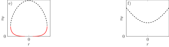
$$\hskip 27.0pt\frac{g_{\mathrm{BF}}}{g_{\mathrm{B}}}\alpha_{\mathrm{B}}-\alpha_{\mathrm{F}}>0\hskip 196.0pt\frac{g_{\mathrm{BF}}}{g_{\mathrm{B}}}\alpha_{\mathrm{B}}-\alpha_{\mathrm{F}}<0$$

Figure 5: Classification of the solutions of Eq. (3.21). The conditions Eq. (3.40)-(3.42) for the number of solutions at the origin are used in combination with geometric arguments based on the conditions Eq. (4.44) and (4.45) in order to determine the six different qualitative fermionic density profiles.

5 Classification of density configurations

In the preceding section we were able to provide a full classification of solutions to Eq. (3.21) with the help of geometric arguments. When we apply the same reasoning to Eq. (3.22), a problem arises, which will be discussed next. The left-hand side of Eq. (3.22) corresponds to a straight line with negative slope for $g_{\mathrm{BF}}>0$ and positive slope for $g_{\mathrm{BF}}<0$, while the right-hand side is a convex function. The solutions of Eq. (3.22) are then identified by the values of $n_{\mathrm{B}}$ where the two functions intersect. The next step in Sec. 4 was to increase the potential in Eq. (3.21) and to track the change of the intersection points in order to obtain the qualitative, spatial dependency of the solutions. However, in Eq. (3.22) both sides depend on $V$, that is, both the convex function and the straight line change as the potential varies, but in possibly different directions and we cannot infer how the value of the intersection point changes. The classification of fermionic solutions has, nevertheless, already provided us with a lot of information about the bosonic solutions. Indeed, it follows from Eq. (2.9) that they will exhibit ceasing and tangent points at the same locations as the fermionic solutions, just as the number of fermionic and bosonic solution branches at every point $\mathbf{r}$ is the same. Since the value of the bosonic solutions at these points may be negative, as can be seen from Eq. (2.9), in order to correspond to a physical solution, its positivity has to be checked explicitly. We will address these problems in A. The calculations in this appendix are somewhat technical, the reader who is mainly interested in the classification of density profiles can skip the details. First, in A.1 we recall the condition for two solutions at the origin and subsequently establish further conditions to specify the sign of $n_{\mathrm{B}}$. In the second step in A.2 we make analytical statements about the value of the bosonic solution at ceasing, tangent and stationary points (the derivative of the bosonic solution becomes zero). These two steps will provide us with all the information we need for a full classification.
Before we start to discuss the different scenarios, let us first make a few general remarks. As mentioned before, we focus on a classification of continuous density profiles. If the fermionic solution branch disappears at a connection point e.g. in Fig. 5.a, d or e, the bosonic solution has to be smaller than zero at this point. If this were not the case, it would not be possible to continuously connect the solution to the pure region, where only one species is present. Contrary to that, at a fermionic ceasing point, e.g. in Fig. 5.b, d or e the bosonic solution can be positive, if this point is the border to the pure bosonic region, or negative, then the point at which the bosonic solution branch crosses zero is the border to the pure fermionic solution. In the conditions we use the abbreviations

$$\beta=\kappa\left(\gamma\frac{\alpha_{\mathrm{B}}}{\alpha_{\mathrm{F}}}\frac{\kappa}{g_{\mathrm{BF}}}\right)^{\frac{\gamma}{1-\gamma}}\quad\quad\text{and}\quad\quad\chi=\kappa\left(\frac{g_{\mathrm{B}}\kappa\gamma}{g^{2}_{\mathrm{BF}}}\right)^{\frac{\gamma}{1-\gamma}}\;,$$ (5.47)

defined in Eq. (3.43) and A.63 for better readability.

5.1 Classification for repulsive interaction $g_{\mathrm{BF}}>0$

Keeping these remarks in mind, we proceed as described in the following. Choosing a fermionic scenario in Fig. 5 defines the number of fermionic and therefore bosonic solutions at the origin. A provides further conditions, which determine their sign at the origin and their values at ceasing, tangent, and stationary points.

5.1.1 Fermionic scenario Fig. 5.a and Fig. 5.b

We start with the fermionic scenarios depicted in Fig. 5.a and 5.b, which both feature two solutions at the origin. If the greater and therefore stable bosonic solution is larger than zero, that is, the additional conditions below Fig. 6.b or 6.c are satisfied, the configuration exhibits a mixed region at the origin. Let us discuss Fig. 5.b first. Here, we observe a ceasing point, which will also be found in the bosonic solution. If the value of the bosonic ceasing point is smaller than zero, that is $\mu_{\mathrm{F}}-\frac{\alpha_{\mathrm{F}}}{\alpha_{\mathrm{B}}}\mu_{\mathrm{B}}>0$ in Eq. (A.57), the bosonic density reaches zero before the fermionic does. The point where the bosonic density becomes zero determines the border of the mixed region to the pure fermionic region. If a stationary point exists due to Eq. (A.64), it will be found in the bosonic solution branch which corresponds to the fermionic branch with negative slope because of Eq. (A.65). This is the stable solution. Furthermore, it follows from Eq. (A.58) that the slope at the ceasing point is negative in the direction of increasing $V$. As there is only one stationary point additionally to the one at the origin, it has to be a maximum. This either leads to scenario 1.1.1 or scenario 1.1.2. If the ceasing point in contrast is larger than zero, $\mu_{\mathrm{F}}-\frac{\alpha_{\mathrm{F}}}{\alpha_{\mathrm{B}}}\mu_{\mathrm{B}}<0$ is true. Following along the same lines as before, we can easily convince ourselves that we find scenario 1.2.1 and scenario 1.2.2.
Before we discuss Fig. 5.b in combination with condition Fig. 6.a, let us turn to Fig. 5.a, where we observe a tangent point but no ceasing point, first again in combination with Fig. 6.b or 6.c. In Fig. 5.a the fermionic density does not reach zero. Consequently, in order to represent a physically reasonable configuration the bosonic tangent point has to be smaller than zero to delimit the mixed region. This is ensured by using Eq. (A.60). Since $\frac{\partial n_{\mathrm{F}}}{\partial V}>0$ everywhere, Eq. (A.65) cannot be satisfied and there is no stationary point. In summary, we find scenario 1.3.
Let us now discuss Fig. 5.a in the context of the conditions of Fig. 6.a. It is easy to convince ourselves that there is no physical scenario with this fermionic density. As the stable fermionic solution does never become zero, for a physically reasonable scenario, the bosonic solution, which is smaller than zero at the origin, should increase, cross zero and then decrease until it reaches zero again. This, however, would imply the existence of a stationary point, which contradicts Eq. (A.65).
Contrary to that, Fig. 5.b in combination with the conditions of Fig. 6.a leads to further scenarios. At the origin the bosonic solution is smaller than zero, however, as the potential increases it might become larger and eventually cross zero, leading to a mixed region.

1. $g_{\mathrm{BF}}>0$, mixed region at the origin

$$\chi\left(1-\gamma\right)>\left(\mu_{\mathrm{F}}-\frac{g_{\mathrm{BF}}}{g_{\mathrm{B}}}\mu_{\mathrm{B}}\right)>0$$

$$\frac{\kappa^{\frac{1}{\gamma}}\mu_{\mathrm{B}}}{g_{\mathrm{BF}}}>\mu_{\mathrm{F}}^{\frac{1}{\gamma}}\quad\text{or}\quad\left[\frac{\kappa^{\frac{1}{\gamma}}\mu_{\mathrm{B}}}{g_{\mathrm{BF}}}<\mu_{\mathrm{F}}^{\frac{1}{\gamma}}\quad\text{and}\quad\frac{1}{\gamma}\mu_{\mathrm{F}}^{\frac{1}{\gamma}-1}>\frac{\kappa^{\frac{1}{\gamma}}g_{\mathrm{B}}}{g_{\mathrm{BF}}^{2}}\right]$$

1.1 Fermionic density decreases, the bosonic density reaches zero first

$$\frac{g_{\mathrm{BF}}}{g_{\mathrm{B}}}\alpha_{\mathrm{B}}-\alpha_{\mathrm{F}}<0,\quad\mu_{\mathrm{F}}-\frac{\alpha_{\mathrm{F}}}{\alpha_{\mathrm{B}}}\mu_{\mathrm{B}}>0$$

1.1.1 No stationary point

$$g_{\mathrm{B}}\mu_{\mathrm{F}}-g_{\mathrm{BF}}\mu_{\mathrm{B}}+\beta\left(g_{\mathrm{BF}}\gamma\frac{\alpha_{\mathrm{B}}}{\alpha_{\mathrm{F}}}-g_{\mathrm{B}}\right)<0$$

1.1.2 Stationary point

$$g_{\mathrm{B}}\mu_{\mathrm{F}}-g_{\mathrm{BF}}\mu_{\mathrm{B}}+\beta\left(g_{\mathrm{BF}}\gamma\frac{\alpha_{\mathrm{B}}}{\alpha_{\mathrm{F}}}-g_{\mathrm{B}}\right)>0$$

1.2 Fermionic density decreases and reaches zero first

$$\frac{g_{\mathrm{BF}}}{g_{\mathrm{B}}}\alpha_{\mathrm{B}}-\alpha_{\mathrm{F}}<0,\quad\mu_{\mathrm{F}}-\frac{\alpha_{\mathrm{F}}}{\alpha_{\mathrm{B}}}\mu_{\mathrm{B}}<0$$

1.2.1 No stationary point

$$\,g_{\mathrm{B}}\mu_{\mathrm{F}}-g_{\mathrm{BF}}\mu_{\mathrm{B}}+\beta\left(g_{\mathrm{BF}}\gamma\frac{\alpha_{\mathrm{B}}}{\alpha_{\mathrm{F}}}-g_{\mathrm{B}}\right)<0$$

1.2.2 Stationary point

$$g_{\mathrm{B}}\mu_{\mathrm{F}}-g_{\mathrm{BF}}\mu_{\mathrm{B}}+\beta\left(g_{\mathrm{BF}}\gamma\frac{\alpha_{\mathrm{B}}}{\alpha_{\mathrm{F}}}-g_{\mathrm{B}}\right)>0$$

1.3 Fermionic density increases in the mixed region

$$\frac{g_{\mathrm{BF}}}{g_{\mathrm{B}}}\alpha_{\mathrm{B}}-\alpha_{\mathrm{F}}>0,\quad\chi\left(\gamma\frac{g_{\mathrm{B}}}{g_{\mathrm{BF}}}-\frac{\alpha_{\mathrm{B}}}{\alpha_{\mathrm{F}}}\right)+\frac{\alpha_{\mathrm{B}}}{\alpha_{\mathrm{F}}}\mu_{\mathrm{F}}-\mu_{\mathrm{B}}<0$$

There are two ways to achieve that. First, we choose $\mu_{\mathrm{F}}-\frac{\alpha_{\mathrm{F}}}{\alpha_{\mathrm{B}}}\mu_{\mathrm{B}}<0$ in Eq. (A.57), so that the value of the ceasing point is larger than zero. As a result of Eq. (A.58) the slope at the ceasing point is negative, leading to a stationary point. Consequently, we find scenario 2.1. Secondly, if we choose $\mu_{\mathrm{F}}-\frac{\alpha_{\mathrm{F}}}{\alpha_{\mathrm{B}}}\mu_{\mathrm{B}}>0$ the ceasing point is below zero. In order to be physical, there has to be a stationary point, that is, Eq. (A.64) has to be true, and its value has to be above zero, which is guaranteed by Eq. (A.62). In summary, we find scenario 2.2.

2. $g_{\mathrm{BF}}>0$, zero bosonic density at the origin

$$\chi\left(1-\gamma\right)>\left(\mu_{\mathrm{F}}-\frac{g_{\mathrm{BF}}}{g_{\mathrm{B}}}\mu_{\mathrm{B}}\right)>0$$

$$\frac{\kappa^{\frac{1}{\gamma}}\mu_{\mathrm{B}}}{g_{\mathrm{BF}}}<\mu_{\mathrm{F}}^{\frac{1}{\gamma}},\quad\frac{1}{\gamma}\mu_{\mathrm{F}}^{\frac{1}{\gamma}-1}<\frac{\kappa^{\frac{1}{\gamma}}g_{\mathrm{B}}}{g_{\mathrm{BF}}^{2}}$$

2.1 Fermionic density reaches zero first

$$\frac{g_{\mathrm{BF}}}{g_{\mathrm{B}}}\alpha_{\mathrm{B}}-\alpha_{\mathrm{F}}<0,\quad\mu_{\mathrm{F}}-\frac{\alpha_{\mathrm{F}}}{\alpha_{\mathrm{B}}}\mu_{\mathrm{B}}<0$$

2.2 Bosonic density reaches zero first

$$\frac{g_{\mathrm{BF}}}{g_{\mathrm{B}}}\alpha_{\mathrm{B}}-\alpha_{\mathrm{F}}<0,\quad\mu_{\mathrm{F}}-\frac{\alpha_{\mathrm{F}}}{\alpha_{\mathrm{B}}}\mu_{\mathrm{B}}>0$$

$$\mu_{\mathrm{F}}-\frac{\alpha_{\mathrm{F}}}{\alpha_{\mathrm{B}}}\mu_{\mathrm{B}}<\beta(1-\gamma)$$

$$g_{\mathrm{B}}\mu_{\mathrm{F}}-g_{\mathrm{BF}}\mu_{\mathrm{B}}+\beta\left(g_{\mathrm{BF}}\gamma\frac{\alpha_{\mathrm{B}}}{\alpha_{\mathrm{F}}}-g_{\mathrm{B}}\right)>0$$

There is a second set of parameters for scenario 2.1 and 2.2, which are

$$\chi\left(1-\gamma\right)<\left(\mu_{\mathrm{F}}-\frac{g_{\mathrm{BF}}}{g_{\mathrm{B}}}\mu_{\mathrm{B}}\right)$$

$$\frac{g_{\mathrm{BF}}}{g_{\mathrm{B}}}\alpha_{\mathrm{B}}-\alpha_{\mathrm{F}}<0,\quad\mu_{\mathrm{F}}-\frac{\alpha_{\mathrm{F}}}{\alpha_{\mathrm{B}}}\mu_{\mathrm{B}}<0$$

$$\chi\left(\gamma\frac{g_{\mathrm{B}}}{g_{\mathrm{BF}}}-\frac{\alpha_{\mathrm{B}}}{\alpha_{\mathrm{F}}}\right)+\frac{\alpha_{\mathrm{B}}}{\alpha_{\mathrm{F}}}\mu_{\mathrm{F}}-\mu_{\mathrm{B}}>0$$

$$\chi\left(1-\gamma\right)<\left(\mu_{\mathrm{F}}-\frac{g_{\mathrm{BF}}}{g_{\mathrm{B}}}\mu_{\mathrm{B}}\right)$$

$$\frac{g_{\mathrm{BF}}}{g_{\mathrm{B}}}\alpha_{\mathrm{B}}-\alpha_{\mathrm{F}}<0,\quad\mu_{\mathrm{F}}-\frac{\alpha_{\mathrm{F}}}{\alpha_{\mathrm{B}}}\mu_{\mathrm{B}}>0$$

$$\chi\left(\gamma\frac{g_{\mathrm{B}}}{g_{\mathrm{BF}}}-\frac{\alpha_{\mathrm{B}}}{\alpha_{\mathrm{F}}}\right)+\frac{\alpha_{\mathrm{B}}}{\alpha_{\mathrm{F}}}\mu_{\mathrm{F}}-\mu_{\mathrm{B}}>0$$

$$\mu_{\mathrm{F}}-\frac{\alpha_{\mathrm{F}}}{\alpha_{\mathrm{B}}}\mu_{\mathrm{B}}<\beta(1-\gamma)$$

$$g_{\mathrm{B}}\mu_{\mathrm{F}}-g_{\mathrm{BF}}\mu_{\mathrm{B}}+\beta\left(g_{\mathrm{BF}}\gamma\frac{\alpha_{\mathrm{B}}}{\alpha_{\mathrm{F}}}-g_{\mathrm{B}}\right)>0$$

5.1.2 Fermionic scenario Fig. 5.c and Fig. 5.d

The next step is to consider the fermionic scenarios Fig. 5.c and 5.d but clearly only the latter leads to a physical configuration. Hence, $\frac{g_{\mathrm{BF}}}{g_{\mathrm{B}}}\alpha_{\mathrm{B}}-\alpha_{\mathrm{F}}<0$ and a ceasing as well as tangent point exist. When we require the ceasing point to be greater and the tangent point to be smaller than zero by means of Eq. (A.57) and Eq. (A.60), we find a second set of parameters for scenario 2.1. If, in contrast, the ceasing and tangent point are both smaller than zero, we have to require a stationary point and it has to be above zero. Using Eq. (A.62) and Eq. (A.64), this leads to a second set of parameters for scenario 2.2.

5.1.3 Fermionic scenario Fig. 5.e and Fig. 5.f

It is left to investigate the case of Fig. 5.e and Fig. 5.f but clearly only the former can lead to a physical situation as the solution in Fig. 5.f is unstable everywhere. Thus, $\frac{g_{\mathrm{BF}}}{g_{\mathrm{B}}}\alpha_{\mathrm{B}}-\alpha_{\mathrm{F}}>0$. As the positive slope of the stable fermionic solution branch prohibits a bosonic stationary point, the ceasing point has to be larger and the tangent point smaller than zero, ensured by Eq. (A.57) and Eq. (A.60). Therefore, we arrive at scenario 3.

3. $g_{\mathrm{BF}}>0$, zero fermionic density at the origin

$$\vspace{-0.15cm}\mu_{\mathrm{F}}-\frac{g_{\mathrm{BF}}}{g_{\mathrm{B}}}\mu_{\mathrm{B}}<0$$

$$\vspace{-0.15cm}\mu_{\mathrm{F}}-\frac{\alpha_{\mathrm{F}}}{\alpha_{\mathrm{B}}}\mu_{\mathrm{B}}>0,\quad\frac{g_{\mathrm{BF}}}{g_{\mathrm{B}}}\alpha_{\mathrm{B}}-\alpha_{\mathrm{F}}>0$$

$$\vspace{-0.15cm}\chi\left(\gamma\frac{g_{\mathrm{B}}}{g_{\mathrm{BF}}}-\frac{\alpha_{\mathrm{B}}}{\alpha_{\mathrm{F}}}\right)+\frac{\alpha_{\mathrm{B}}}{\alpha_{\mathrm{F}}}\mu_{\mathrm{F}}-\mu_{\mathrm{B}}<0$$

5.2 Classification for attractive interaction $g_{\mathrm{BF}}<0$

We now turn to the situation where $g_{\mathrm{BF}}<0$. While the geometric arguments we used to obtain the fermionic solutions in Fig. 5 are still valid, the discussion in A.1 is not due to the change of sign of $g_{\mathrm{BF}}$ in Eq. (A.50). As it will turn out, there are only two distinct scenarios here, which we will be able to obtain by the results of A.2 that are valid for both signs of $g_{\mathrm{BF}}$. It is important to note that according to Eq. (3.28) now the lower fermionic and the lower bosonic solution correspond to the stable density, whereas the upper bosonic solution is now unstable. From the conditions in Fig. 5 we recognize that $g_{\mathrm{BF}}<0$ is only compatible with Fig. 5.b, d and f but obviously Fig. 5.f does not lead to a physical configuration. In these cases $\frac{g_{\mathrm{BF}}}{g_{\mathrm{B}}}\alpha_{\mathrm{B}}-\alpha_{\mathrm{F}}<0$ is always true. Recall from the discussion in A.2 that if $g_{\mathrm{BF}}<0$, there is no stationary point.
We will first investigate the bosonic solution corresponding to Fig. 5.d. This solution shows a tangent point and a ceasing point. In order to result in a reasonable density, we have to require that the bosonic tangent point is smaller than zero. When we recall that the slope of the bosonic solution branch at the ceasing point is negative due to Eq. (A.58) and that there is no stationary point, it follows that $n_{\mathrm{B}}<0$ everywhere and we therefore conclude that Fig. 5.d for $g_{\mathrm{BF}}<0$ does not lead to a physical density distribution.

4. $g_{\mathrm{BF}}<0$

$$\chi\left(1-\gamma\right)>\left(\mu_{\mathrm{F}}-\frac{g_{\mathrm{BF}}}{g_{\mathrm{B}}}\mu_{\mathrm{B}}\right)$$ (5.48)

4.1 Fermionic density reaches zero first

$$\mu_{\mathrm{F}}-\frac{\alpha_{\mathrm{F}}}{\alpha_{\mathrm{B}}}\mu_{\mathrm{B}}<0$$

4.2 Bosonic density reaches zero first

$$\mu_{\mathrm{F}}-\frac{\alpha_{\mathrm{F}}}{\alpha_{\mathrm{B}}}\mu_{\mathrm{B}}>0$$

If the conditions of Fig. 5.b are fulfilled we observe a ceasing point. We first show that $n_{\mathrm{B}}>0$ at the origin. To this end, we cast Eq. (2.9) in the form

$$n_{\mathrm{B}}=\frac{1}{g_{\mathrm{B}}}\left(\mu_{\mathrm{B}}+|g_{\mathrm{BF}}|n_{\mathrm{F}}\right)>0\;.$$ (5.49)

Depending on whether we choose the ceasing point above or below zero, we find two distinct configurations, namely scenario 4.1 and 4.2
We show in C that neither full nor partial phase separation can occur in the case of attractive interaction. Thus, if the parameters do not allow the continuous configurations 4.1 or 4.2, there is no stable configuration possible and the system collapses, which happens exactly if Eq. (5.48) is violated. This condition has already been obtained by Refs. [22, 20] in order to determine the unstable regime in parameter space.
It is important to note that all the configurations described in this section are minima of the grand-canonical energy. Stability in the mixed region is guaranteed by selecting the stable solution branch in Sec. 3. We show in B that the configurations are also stable with respect to density variations in the pure regions.

6 Conclusion

We have presented a complete classification of all continuous ground-sate density configurations of a boson-fermion mixture at zero temperature. The results of this paper are valid for spin-polarized fermions or for a superfluid mixture at unitarity. We have assumed the bosons to interact among themselves and with the fermions via s-wave scattering. In contrast, the interaction between the fermions can be neglected at extremely low temperatures. The system is trapped by a potential, which can be quite general, in particular it is not necessarily harmonic: It only has to be continuous and monotonous along every direction. We have started from the mean-field grand-canonical energy functional, where the local-density approximation for fermions has been employed. In addition, we have neglected the bosonic kinetic-energy term in the spirit of the Thomas-Fermi approximation. It has been shown that the binary form of the system allows three different regions, which have to be treated separately: A mixed region, where the bosonic and fermionic densities overlap, and two pure regions where only one species is present. We have referred to the possible density configurations as ‘fully phase separated’, if no mixed region exists, here one expects in general discontinuities in the densities, ‘partially phase separated’ if a mixed region exists but there is at least one discontinuity, and ‘continuous’ if the densities are continuous. We have briefly discussed phase separation in the context a mixture with attractive inter-species interaction, where we showed that phase separated configurations are not stable. This explains the onset of collapse in these systems when the choice of parameters do not allow continuous configurations.
In this paper we have investigated in detail continuous density profiles, which led to numerous scenarios. By taking the first variation of the grand-canonical energy functional, we have obtained coupled equations for the bosonic and fermionic density, respectively. The equations could be decoupled but are still nonlinear in the mixed region, giving rise to in general several solution branches. Remarkably, we have shown that the stability conditions for the coexisting region, resultant from the second variation of the energy functional, can be used to select, if existent, the stable solution branch, which is then unique. In the following course of constructing the density shapes we have pursued a geometric approach, that is, by trying to understand the behavior of the equations, conditions could be derived to first determine six different classes of fermionic density shapes. By additionally including analytic results about, for instance, the existence of maxima in the bosonic density or which species encloses the other, we were also able to establish the shape of the bosonic densities in the coexisting region. These could then be complemented by the solutions in the pure regions to finally obtain in total ten different configurations. Finally, we have proved that every continuous configuration constructed in this manner is also stable with respect to density variations in the pure regions.
To our knowledge scenario 2.2 has not yet been described in the literature. This configurations consists of a shell of bosons completely enclosed by the fermionic cloud. It is the only density shape with two distinct pure regions of the same species. This feature is a manifestation of the nonlinearity of the equation as discussed in B. Our results can also be applied to a binary mixture of bosons by taking the limit $\gamma\rightarrow 1$ in all the conditions. It is worthwhile noting that most of the configurations we find for the boson-fermion mixture are also possible in a binary mixture of bosons. There are two exceptions namely scenario 1.1.2 and 2.2 which cannot occur in this case.
In conclusion, we have developed a rigorous and comprehensive classification scheme for the ground-state density profiles of a boson-fermion mixture with spin-polarized fermions and we have analytically proved stability for all the configurations that we describe.

Appendix A Qualitative shape of the bosonic solutions for $g_{\mathrm{BF}}>0$

As described in Sec. 5, the form of Eq. (3.22) does not permit to predict the qualitative shape of the bosonic solutions by the same simple arguments as used in Sec. 4 for the fermionic classification. Complementing the discussion with the additional analytic conditions derived in this appendix, we will be able to determine the bosonic density shapes as well. First, in the case of two solutions at the origin their sign is determined in A.1, followed by A.2 where we determine the values of the bosonic density at ceasing, tangent, and stationary points.

A.1 Sign of bosonic solutions at the origin ($V=0$)

At the origin $V=0$ and Eq. (3.22) takes the simpler form

$$\frac{\kappa^{\frac{1}{\gamma}}\mu_{\mathrm{B}}}{g_{\mathrm{BF}}}-\frac{\kappa^{\frac{1}{\gamma}}g_{\mathrm{B}}}{g_{\mathrm{BF}}}n_{\mathrm{B}}=\left(\mu_{\mathrm{F}}-g_{\mathrm{BF}}n_{\mathrm{B}}\right)^{\frac{1}{\gamma}}\;.$$ (A.50)

This equation exhibits zero, one, or two real solutions. The case studied in this section is two solutions for which Eq. (3.41) with $V=0$ provides the condition

$$\chi\left(1-\gamma\right)>\left(\mu_{\mathrm{F}}-\frac{g_{\mathrm{BF}}}{g_{\mathrm{B}}}\mu_{\mathrm{B}}\right)>0\;.$$ (A.51)

The left-hand side of Eq. (A.50) is interpreted as a straight line with negative slope (for $g_{\mathrm{BF}}>0$), the right-hand side as a convex function. The solutions for $n_{\mathrm{B}}$ at the origin are again given by the intersection points of these two functions. Depending on the sign of the solutions, there can be three subcases, i.e. two negative, two positive, or one positive and one negative solution. These situations are illustrated in Fig. 6.a-6.c. In the following we derive conditions to distinguish these three cases by comparing the ordinate intersection of the two functions, given by $\frac{\kappa^{\frac{1}{\gamma}}\mu_{\mathrm{B}}}{g_{\mathrm{BF}}}$ for the straight line and by $\mu_{\mathrm{F}}^{\frac{1}{\gamma}}$ for the convex function as can be seen from Eq. (A.50) by setting $n_{\mathrm{B}}=0$. Thus, if $\frac{\kappa^{\frac{1}{\gamma}}\mu_{\mathrm{B}}}{g_{\mathrm{BF}}}<\mu_{\mathrm{F}}^{\frac{1}{\gamma}}$ the straight line crosses the ordinate below the convex function e.g. in Fig. 6.a and 6.b, while, in contrast, for $\frac{\kappa^{\frac{1}{\gamma}}\mu_{\mathrm{B}}}{g_{\mathrm{BF}}}>\mu_{\mathrm{F}}^{\frac{1}{\gamma}}$ we observe the behavior depicted in Fig. 6.c.
In the case of $\frac{\kappa^{\frac{1}{\gamma}}\mu_{\mathrm{B}}}{g_{\mathrm{BF}}}<\mu_{\mathrm{F}}^{\frac{1}{\gamma}}$, there are either two negative (Fig. 6.a) or two positive solutions (Fig. 6.b). In order to distinguish between these two situations, we compare the slope of the straight line with the slope of the convex function at $n_{\mathrm{B}}=0$ and find two positive solutions if the slope of the straight line is greater than the first derivative of the convex function, which means

$$\frac{1}{\gamma}\mu_{\mathrm{F}}^{\frac{1}{\gamma}-1}>\frac{\kappa^{\frac{1}{\gamma}}g_{\mathrm{B}}}{g_{\mathrm{BF}}^{2}}\;.$$ (A.52)

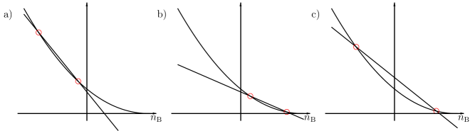
$$\frac{\kappa^{\frac{1}{\gamma}}\mu_{\mathrm{B}}}{g_{\mathrm{BF}}} <\mu_{\mathrm{F}}^{\frac{1}{\gamma}}\qquad\qquad\qquad \frac{\kappa^{\frac{1}{\gamma}}\mu_{\mathrm{B}}}{g_{\mathrm{BF}}} <\mu_{\mathrm{F}}^{\frac{1}{\gamma}}\qquad\qquad\quad\quad\qquad \frac{\kappa^{\frac{1}{\gamma}}\mu_{\mathrm{B}}}{g_{\mathrm{BF}}}>\mu_{\mathrm{F}}^{\frac{1}{\gamma}}$$ (A.53)

$$\frac{1}{\gamma}\mu_{\mathrm{F}}^{\frac{1}{\gamma}-1} <\frac{\kappa^{\frac{1}{\gamma}}g_{\mathrm{B}}}{g_{\mathrm{BF}}^{2}}\qquad\qquad\qquad \frac{1}{\gamma}\mu_{\mathrm{F}}^{\frac{1}{\gamma}-1} >\frac{\kappa^{\frac{1}{\gamma}}g_{\mathrm{B}}}{g_{\mathrm{BF}}^{2}}$$

Figure 6: Geometric solution to Eq. (3.22). Depending on the conditions Eq. (A.53), two negative (Fig. 6.a), two positive (Fig. 6.b), or one positive and one negative bosonic solutions (Fig. 6.c) emerge at the origin.

Similarly, we find two negative solutions if the slope of the straight line is smaller than the first derivative of the convex function, i.e.

$$\frac{1}{\gamma}\mu_{\mathrm{F}}^{\frac{1}{\gamma}-1}<\frac{\kappa^{\frac{1}{\gamma}}g_{\mathrm{B}}}{g_{\mathrm{BF}}^{2}}\;.$$ (A.54)

Below Fig. 6 we have summarized the additional conditions to specify the sign of the bosonic solutions at the origin in the case of two real solutions.

A.2 Values of $n_{\mathrm{B}}$ at ceasing, tangent, and stationary points

We complete this appendix by deriving conditions for the existence and the values of ceasing, tangent, and stationary points in the bosonic solutions.
Ceasing points:          
When both functions e.g. in Fig. 6.a move to the left as $V$ is varied, but the straight line is ‘slower’, there exists a $V^{(0)}$ where the upper solution branch ceases and there is no solution for $V>V^{(0)}$ anymore. This happens exactly when the right-hand side and the left-hand side of Eq. (3.22) are simultaneously zero at the same point $n_{\mathrm{B}}^{(0)}$, giving rise to the system of equations

$$\alpha_{\mathrm{B}}V^{(0)}\;+\;g_{\mathrm{B}}\;n_{\mathrm{B}}^{(0)}-\mu_{\mathrm{B}}=0$$ (A.55)

$$\alpha_{\mathrm{F}}V^{(0)}\;+\;g_{\mathrm{BF}}n_{\mathrm{B}}^{(0)}-\mu_{\mathrm{F}}=0$$ (A.56)

with the solution

$$n_{\mathrm{B}}^{(0)}=\frac{\alpha_{\mathrm{B}}}{g_{\mathrm{B}}}\;\frac{\mu_{\mathrm{F}}-\frac{\alpha_{\mathrm{F}}}{\alpha_{\mathrm{B}}}\mu_{\mathrm{B}}}{\frac{g_{\mathrm{BF}}}{g_{\mathrm{B}}}\alpha_{\mathrm{B}}-\alpha_{\mathrm{F}}}\,.$$ (A.57)

When we take the derivative of Eq. (3.22) with respect to $$V$$ at the ceasing point, we find

$$\frac{\partial n_{\mathrm{B}}^{(0)}}{\partial V}=-\frac{\alpha_{\mathrm{B}}}{g_{\mathrm{B}}}\,.$$ (A.58)

Therefore, the bosonic density decreases at a ceasing point in the direction of increasing $V$. Moreover, it is worthwhile noting that if a ceasing point exists, it is in the upper bosonic solution as can easily be seen from Fig. 6.

Tangent points:          
If the straight line moves ‘faster’, the two intersection points approach each other until they combine. At this point $V^{(t)}$ the straight line is tangent to the convex function. Here, the two solution branches connect and there is no real solution for $V>V^{(t)}$. Thus, in addition to satisfying Eq. (3.22) we require the derivative with respect to $n_{\mathrm{B}}$ of its left-hand side and the derivative of its right-hand side to be equal at constant $V$. After rearranging terms, this reads

$$\chi=\mu_{\mathrm{F}}-V^{(t)}_{\mathrm{F}}-g_{\mathrm{BF}}n_{\mathrm{B}}^{(t)}\;,$$ (A.59)

where we have recalled Eq. (3.43). Again, Eq. (3.22) and Eq. (A.59) constitute a system of equations promoting the solution

$$n_{\mathrm{B}}^{(t)}=\frac{\alpha_{\mathrm{F}}}{g_{\mathrm{B}}}\;\frac{\chi\left(\gamma\frac{g_{\mathrm{B}}}{g_{\mathrm{BF}}}-\frac{\alpha_{\mathrm{B}}}{\alpha_{\mathrm{F}}}\right)+\frac{\alpha_{\mathrm{B}}}{\alpha_{\mathrm{F}}}\mu_{\mathrm{F}}-\mu_{\mathrm{B}}}{\frac{g_{\mathrm{BF}}}{g_{\mathrm{B}}}\alpha_{\mathrm{B}}-\alpha_{\mathrm{F}}}\;.$$ (A.60)

Stationary points:          
In order to completely capture the behavior of the bosonic solutions, we have to investigate if $n_{\mathrm{B}}$ exhibits stationary points, that is, if there exists a $V^{(s)}>0$ with $\partial n_{\mathrm{B}}^{(s)}/\partial V=0$. When we take the derivative with respect to $V$ on both sides of Eq. (3.22) and set $\partial n_{\mathrm{B}}^{(s)}/\partial V=0$, we obtain

$$\frac{\alpha_{\mathrm{B}}}{\alpha_{\mathrm{F}}}\gamma\frac{\kappa^{\frac{1}{\gamma}}}{g_{\mathrm{BF}}}=\left(\mu_{\mathrm{F}}-V_{\mathrm{F}}^{(s)}-g_{\mathrm{BF}}n_{\mathrm{B}}^{(s)}\right)^{\frac{1}{\gamma}-1}\;.$$ (A.61)

Clearly, there is no solution to this equation if $g_{\mathrm{BF}}<0$, thus there will be no stationary point in the case of attractive inter-species interaction. For repulsive interaction the system of Eq. (3.22) and Eq. (A.61) admits the solution

$$n_{\mathrm{B}}^{(s)}=\frac{\alpha_{\mathrm{B}}}{g_{\mathrm{B}}\left(\frac{g_{\mathrm{BF}}}{g_{\mathrm{B}}}\alpha_{\mathrm{B}}-\alpha_{\mathrm{F}}\right)}\left[\mu_{\mathrm{F}}-\frac{\alpha_{\mathrm{F}}}{\alpha_{\mathrm{B}}}\mu_{\mathrm{B}}-\beta\left(1-\gamma\right)\right]\;.$$ (A.62)

Here we have defined the parameter

$$\beta:=\kappa\left(\gamma\frac{\alpha_{\mathrm{B}}}{\alpha_{\mathrm{F}}}\frac{\kappa}{g_{\mathrm{BF}}}\right)^{\frac{\gamma}{1-\gamma}}\;.$$ (A.63)

Thus, a stationary point additionally to the one at the origin exist if

$$-V^{(s)}=\frac{1}{g_{\mathrm{B}}\left(\frac{g_{\mathrm{BF}}}{g_{\mathrm{B}}}\alpha_{\mathrm{B}}-\alpha_{\mathrm{F}}\right)}\left[g_{\mathrm{B}}\mu_{\mathrm{F}}-g_{\mathrm{BF}}\mu_{\mathrm{B}}+\beta\left(g_{\mathrm{BF}}\gamma\frac{\alpha_{\mathrm{B}}}{\alpha_{\mathrm{F}}}-g_{\mathrm{B}}\right)\right]<0\,.$$ (A.64)

When we take the derivative with respect to $V$ of Eq. (2.9) and set $\partial n_{\mathrm{B}}^{(s)}/\partial V=0$ at the stationary point, we arrive at

$$0=\alpha_{\mathrm{B}}+g_{\mathrm{BF}}\frac{\partial n_{\mathrm{F}}^{(s)}}{\partial V}$$ (A.65)

Obviously, for positive $g_{\mathrm{BF}}$ this can only be true when the fermionic density decreases as $V$ is increased. This argument therefore determines which solution branch becomes stationary.

Appendix B Stability in $\Omega_{\mathrm{B}}$ and $\Omega_{\mathrm{F}}$

In this appendix we show that every scenario with a mixed region and continuous densities is stable with respect to the inequalities Eq. (2.19) and (2.20) in the pure region. We then conclude that every scenario derived in Sec. 5 is stable.
We start by defining

$$f_{\mathrm{B}} :=V_{\mathrm{F}}+g_{\mathrm{BF}}n_{\mathrm{B}}-\mu_{\mathrm{F}}\quad\quad\text{and}$$ (B.66)

$$f_{\mathrm{F}} :=V_{\mathrm{B}}+g_{\mathrm{BF}}n_{\mathrm{F}}-\mu_{\mathrm{B}}\;,$$ (B.67)

so that it remains to show that

$$f_{i} \geq 0\;\;\text{in}\;\;\Omega_{i}\;\;\text{for}\;\;i=\mathrm{B,F}.$$ (B.68)

Note that the functions $$f_{i}$$ are continuous as the potentials and the densities are continuous. Comparing Eq. (B.66) and Eq. (B.67) with Eq. (2.9) and Eq. (2.10) leads to

$$f_{\mathrm{B}} =-\kappa n_{\mathrm{F}}^{\gamma}\quad\quad\text{and}$$ (B.69)

$$f_{\mathrm{F}} =-g_{\mathrm{B}}n_{\mathrm{B}}$$ (B.70)

for $\mathbf{r}\in\Omega_{\mathrm{BF}}$. Thus, $f_{i}$ is smaller than zero in the mixed region and $f_{i}=0$ at the border between $\Omega_{\mathrm{BF}}$ and $\Omega_{i}$ by definition of the pure region. Consequently, $f_{i}$ switches sign from negative to positive at the border between the mixed and the pure region and thus it is left to show that $f_{i}\neq 0$ everywhere else in $\Omega_{i}$. Before we prove that this is indeed true, it is important to note that $n_{i}$ is a monotonous function over the union of all pure regions of species $i$ in the same sense of monotony as defined in Sec. 2. This statement follows from Eq. (2.11) and Eq. (2.12) as the potentials are monotonous. As a consequence, it is sufficient to consider $f_{i}$ a function of $n_{i}$ instead of $\mathbf{r}$.
By writing $V_{\mathrm{B}}=\alpha_{\mathrm{B}}V$ and $V_{\mathrm{F}}=\alpha_{\mathrm{F}}V$, we insert Eq. (2.11) into Eq. (B.66) and Eq. (2.12) into Eq. (B.67) to eliminate the potentials. This leads to the expressions

$$f_{\mathrm{B}} =-\left(\mu_{\mathrm{F}}-\frac{\alpha_{\mathrm{F}}}{\alpha_{\mathrm{B}}}\mu_{\mathrm{B}}\right)+\frac{g_{\mathrm{B}}}{\alpha_{\mathrm{B}}}\left(\frac{g_{\mathrm{BF}}}{g_{\mathrm{B}}}\alpha_{\mathrm{B}}-\alpha_{\mathrm{F}}\right)n_{\mathrm{B}}$$ (B.71)

and

$$f_{\mathrm{F}} =\frac{\alpha_{\mathrm{B}}}{\alpha_{\mathrm{F}}}\left(\mu_{\mathrm{F}}-\frac{\alpha_{\mathrm{F}}}{\alpha_{\mathrm{B}}}\mu_{\mathrm{B}}+\frac{\alpha_{\mathrm{F}}}{\alpha_{\mathrm{B}}}g_{\mathrm{BF}}n_{\mathrm{F}}-\kappa n_{\mathrm{F}}^{\gamma}\right)\;,$$ (B.72)

valid in the pure bosonic and fermionic regions, respectively.
Eq. (B.71) is a linear function of $n_{\mathrm{B}}$ and therefore admits one or no zero. If a border between $\Omega_{\mathrm{BF}}$ and $\Omega_{\mathrm{B}}$ exists, then $f_{\mathrm{B}}$ is negative in $\Omega_{\mathrm{BF}}$, zero at the border, and consequently positive in $\Omega_{\mathrm{B}}$, hence we have proved Eq. (B.68) for $i=\mathrm{B}$.
The argument for $f_{\mathrm{F}}$, on the other hand, is slightly more involved. Nevertheless, when we realize that the right-hand side of Eq. (B.72) is of the same form as Eq. (3.21), provided that $g_{\mathrm{BF}}>0$, we are able to apply the considerations made in Sec. 3.2 according to which a function of this form can have no, one or two zeros. In the case of one zero the pure fermionic region is stable according to the same argument as used for $f_{\mathrm{B}}$. In the case of two zeros, let us determine how $f_{\mathrm{F}}$ behaves for large $n_{\mathrm{F}}$. As $\gamma<1$,

$$f_{\mathrm{F}}\rightarrow\infty\quad\quad\text{for}\quad\quad n_{\mathrm{F}}\rightarrow\infty\;,$$ (B.73)

that is, the function qualitatively looks like as depicted in Fig. 7. Note that $f_{\mathrm{F}}(n_{\mathrm{F}}=0)>0$ since we consider the case of two zeros. Given a border between $\Omega_{\mathrm{BF}}$ and $\Omega_{\mathrm{F}}$, it might correspond to the first or second zero of $f_{\mathrm{F}}$. But irrespectively of that, once a border from the mixed region to the pure fermionic region is crossed, $f_{\mathrm{F}}$ stays larger than zero. It is also readily shown that $f_{\mathrm{F}}$ assumes no or one zero if $g_{\mathrm{BF}}<0$. Thus, we have proved Eq. (B.68) also for $i=\mathrm{F}$.

Figure 7: Qualitative shape of $f_{\mathrm{F}}$ in the case of two zeros.

In summary we have found that all density configurations which are constructed as described in the end of Sec. 2 are (meta-) stable. It is interesting to note that the results of this appendix only allow at most one border between mixed and pure bosonic region but two borders between mixed and pure fermionic region in a given direction. This is exactly what we observe in Sec. 5.1 and Sec. 5.2 where the only configuration with two borders between $\Omega_{\mathrm{BF}}$ and $\Omega_{\mathrm{F}}$ is scenario (2.2).

Appendix C Origin of the collapse in the case of $g_{\mathrm{BF}}<0$

In this appendix we show that $g_{\mathrm{BF}}<0$ precludes phase separation.
Clearly, in this case the components attract each other and the system therefore rather tries to increase the overlap between the densities than tends to separate and demix. But what is clear from physical reasoning can also be shown rigorously.
We begin by noting that for $g_{\mathrm{BF}}<0$ Eq. (B.71) and Eq. (B.72) are monotonically decreasing functions of the respective densities. Depending on the sign of $\mu_{\mathrm{F}}-\frac{\alpha_{\mathrm{F}}}{\alpha_{\mathrm{B}}}\mu_{\mathrm{B}}$, either $f_{\mathrm{B}}$ or $f_{\mathrm{F}}$ only assumes negative values and therefore precludes a pure region for that species. Hence, scenarios with both a pure fermionic and a pure bosonic region do not exist and full phase separation cannot occur.
In the second step we prove that every partially phase separated scenario is unstable as well. To this end, let us assume a mixed region where at a certain point the density of one component suddenly drops to zero, the density of the other species will then show a discontinuity. Exemplarily, we assume that the bosonic density drops to zero, the discontinuity will then emerge in the fermionic density. The proof in case of a bosonic discontinuity goes along similar lines and will therefore not be shown here. Let us now denote all quantities at the discontinuity by the superscript $(d)$ when they correspond to the limit from the pure region and by $(m)$ for the limit from the mixed region. Evaluating Eq. (B.67) at both sides of the discontinuity and subtracting the results from each other yields

$$f_{\mathrm{F}}^{(d)}-f_{\mathrm{F}}^{(m)}=g_{\mathrm{BF}}\left(n_{\mathrm{F}}^{(d)}-n_{\mathrm{F}}^{(m)}\right)\;.$$ (C.74)

We also obtain

$$n_{\mathrm{F}}^{\gamma\;(d)}-n_{\mathrm{F}}^{\gamma\;(m)}=\frac{g_{\mathrm{BF}}}{\kappa}n_{\mathrm{B}}^{(m)}<0$$ (C.75)

from Eq. (2.10) and Eq. (2.12). Note that from the equation above it follows that the density jumps to a greater value at the border from the pure to the mixed region. With the help of the mean-value theorem we rewrite

$$n_{\mathrm{F}}^{\gamma\;(d)}-n_{\mathrm{F}}^{\gamma\;(m)}=\gamma\xi^{\gamma-1}\left(n_{\mathrm{F}}^{(d)}-n_{\mathrm{F}}^{(m)}\right)<\gamma n_{\mathrm{F}}^{\gamma-1\;(m)}\left(n_{\mathrm{F}}^{(d)}-n_{\mathrm{F}}^{(m)}\right)\;,$$ (C.76)

where we have made use of the fact that $\xi\in(n_{\mathrm{F}}^{(d)},n_{\mathrm{F}}^{(m)})$ and $n_{\mathrm{F}}^{(m)}>n_{\mathrm{F}}^{(d)}$. When we substitute Eq. (B.70), into Eq. (C.74), we obtain the relation

$$f_{\mathrm{F}}^{(d)} =-g_{\mathrm{B}}n_{\mathrm{B}}^{(m)}+g_{\mathrm{BF}}\left(n_{\mathrm{F}}^{(d)}-n_{\mathrm{F}}^{(m)}\right)$$

$$<-g_{\mathrm{B}}n_{\mathrm{B}}^{(m)}+\frac{g_{\mathrm{BF}}}{\gamma}n_{\mathrm{F}}^{1-\gamma\;(m)}\left(n_{\mathrm{F}}^{\gamma\;(d)}-n_{\mathrm{F}}^{\gamma\;(m)}\right)$$

$$=g_{\mathrm{B}}n_{\mathrm{B}}^{(m)}n_{\mathrm{F}}^{1-\gamma\;(m)}\left(\frac{g_{\mathrm{BF}}^{2}}{\kappa\gamma g_{\mathrm{B}}}-n_{\mathrm{F}}^{\gamma-1\;(m)}\right)$$

$$<0\;.$$ (C.77)

The first inequality follows from Eq. (C.76) since $g_{\mathrm{BF}}<0$. We then use Eq. (C.75) and the last inequality follows from Eq. (2.18), that is, from the stability of the density in the mixed region.
In summary we have shown that in the case of attractive interaction there are neither stable fully phase-separated nor stable partially phase-separated configurations. When the conditions above scenario 4.1 and 4.2 are not satisfied, then there exists no other stable solution within our model. Indeed, the system collapses as has been experimentally observed by [9].

References

- [1] M. H. Anderson, J. R. Ensher, M. R. Matthews, C. E. Wieman, and E. A. Cornell. Observation of Bose-Einstein Condensation in a Dilute Atomic Vapor. Science, 269:198, 1995.
- [2] K. B. Davis, M. O. Mewes, M. R. Andrews, N. J. van Druten, D. S. Durfee, D. M. Kurn, and W. Ketterle. Bose-Einstein Condensation in a Gas of Sodium Atoms. Phys. Rev. Lett., 75:3969, 1995.
- [3] B. DeMarco, J. L. Bohn, J. P. Burke, M. Holland, and D. S. Jin. Measurement of -Wave Threshold Law Using Evaporatively Cooled Fermionic Atoms. Phys. Rev. Lett., 82:4208, 1999.
- [4] B. DeMarco and D. S. Jin. Onset of Fermi Degeneracy in a Trapped Atomic Gas. Science, 285:1703, 1999.
- [5] F. Schreck, L. Khaykovich, K. L. Corwin, G. Ferrari, T. Bourdel, J. Cubizolles, and C. Salomon. Quasipure Bose-Einstein Condensate Immersed in a Fermi Sea. Phys. Rev. Lett., 87:080403, 2001.
- [6] Z. Hadzibabic, C. A. Stan, K. Dieckmann, S. Gupta, M. W. Zwierlein, A. Görlitz, and W. Ketterle. Two-Species Mixture of Quantum Degenerate Bose and Fermi Gases. Phys. Rev. Lett., 88:160401, 2002.
- [7] A. G. Truscott, K. E. Strecker, W. I. McAlexander, G. B. Partridge, and R. G. Hulet. Observation of Fermi Pressure in a Gas of Trapped Atoms. Science, 291:2570, 2001.
- [8] G. Roati, F. Riboli, G. Modugno, and M. Inguscio. Fermi-Bose Quantum Degenerate Mixture with Attractive Interaction. Phys. Rev. Lett., 89:150403, 2002.
- [9] G. Modugno, G. Roati, F. Riboli, F. Ferlaino, R. J. Brecha, and M. Inguscio. Collapse of a Degenerate Fermi Gas. Science, 297:2240, 2002.
- [10] K. Mølmer. Bose Condensates and Fermi Gases at Zero Temperature. Phys. Rev. Lett., 80:1804, 1998.
- [11] C. Ospelkaus, S. Ospelkaus, K. Sengstock, and K. Bongs. Interaction-Driven Dynamics of Fermion-Boson Gas Mixtures in the Large-Particle-Number Limit. Phys. Rev. Lett., 96:020401, 2006.
- [12] S. Ospelkaus, C. Ospelkaus, L. Humbert, K. Sengstock, and K. Bongs. Tuning of Heteronuclear Interactions in a Degenerate Fermi-Bose Mixture. Phys. Rev. Lett., 97:120403, 2006.
- [13] M. W. Zwierlein, J. R. Abo-Shaeer, A. Schirotzek, C. H. Schunck, and W. Ketterle. Vortices and superfluidity in a strongly interacting Fermi gas. Nature, 435:1047, 2005.
- [14] I. Ferrier-Barbut, M. Delehaye, S. Laurent, A. T. Grier, M. Pierce, B. S. Rem, F. Chevy, and C. Salomon. A mixture of Bose and Fermi superfluids. Science, 345:1035, 2014.
- [15] R. Roth and H. Feldmeier. Mean-field instability of trapped dilute boson-fermion mixtures. Phys. Rev. A, 65:021603, 2002.
- [16] X. Liu, M. Modugno, and H. Hu. Finite-temperature effects on the collapse of trapped Bose-Fermi mixtures. Phys. Rev. A, 68:053605, 2003.
- [17] M. Modugno, F. Ferlaino, F. Riboli, G. Roati, G. Modugno, and M. Inguscio. Mean-field analysis of the stability of a K-Rb Fermi-Bose mixture. Phys. Rev. A, 68:043626, 2003.
- [18] S. K. Adhikari. Mean-field description of a dynamical collapse of a fermionic condensate in a trapped boson-fermion mixture. Phys. Rev. A, 70:043617, 2004.
- [19] A. M. Belemuk, V. N. Ryzhov, and S.-T. Chui. Stable and unstable regimes in Bose-Fermi mixtures with attraction between components. Phys. Rev. A, 76:013609, 2007.
- [20] T. Miyakawa, T. Suzuki, and H. Yabu. Induced instability for boson-fermion mixed condensates of alkali-metal atoms due to the attractive boson-fermion interaction. Phys. Rev. A, 64:033611, 2001.
- [21] T. Karpiuk, M. Brewczyk, M. Gajda, and K. Rza̧żewski. On the stability of Bose–Fermi mixtures. Journal of Physics B, 38:L215, 2005.
- [22] S. Röthel and A. Pelster. Density and stability in ultracold dilute boson-fermion mixtures. The European Physical Journal B, 59:343, 2007.
- [23] N. Nygaard and K. Mølmer. Component separation in harmonically trapped boson-fermion mixtures. Phys. Rev. A, 59:2974, 1999.
- [24] R. Roth. Structure and stability of trapped atomic boson-fermion mixtures. Phys. Rev. A, 66:013614, 2002.
- [25] Z. Akdeniz, A. Minguzzi, P. Vignolo, and M. P. Tosi. Demixing in mesoscopic Boson-Fermion clouds inside cylindrical harmonic traps: Quantum phase diagram and role of temperature. Phys. Rev. A, 66:013620, 2002.
- [26] Z. Akdeniz, P. Vignolo, and M. P. Tosi. Boson–fermion mixtures inside an elongated cigar-shaped trap. Journal of Physics B, 38:2933, 2005.
- [27] L. Viverit, C. J. Pethick, and H. Smith. Zero-temperature phase diagram of binary boson-fermion mixtures. Phys. Rev. A, 61:053605, 2000.
- [28] M. Amoruso, A. Minguzzi, S. Stringari, M. P. Tosi, and L. Vichi. Temperature-dependent density profiles of trapped boson-fermion mixtures. Eur. Phys. J. D, 4:261, 1998.
- [29] Z. Akdeniz, P. Vignolo, A. Minguzzi, and M.P. Tosi. Phase separation in a boson-fermion mixture of lithium atoms. Journal of Physics B, 35:L105, 2002.
- [30] L. Viverit and S. Giorgini. Ground-state properties of a dilute Bose-Fermi mixture. Phys. Rev. A, 66:063604, 2002.
- [31] A. P. Albus, S. A. Gardiner, F. Illuminati, and M. Wilkens. Quantum field theory of dilute homogeneous Bose-Fermi mixtures at zero temperature: General formalism and beyond mean-field corrections. Phys. Rev. A, 65:053607, 2002.
- [32] A. P. Albus, F. Illuminati, and M. Wilkens. Ground-state properties of trapped Bose-Fermi mixtures: Role of exchange correlation. Phys. Rev. A, 67:063606, 2003.
- [33] X. Liu and H. Hu. Collisionless and hydrodynamic excitations of trapped boson-fermion mixtures. Phys. Rev. A, 67:023613, 2003.
- [34] T. L. Ho and V. B. Shenoy. Binary mixtures of Bose condensates of alkali atoms. Phys. Rev. Lett., 77:3276, 1996.
- [35] F. Riboli and M. Modugno. Topology of the ground state of two interacting Bose-Einstein condensates. Phys. Rev. A, 65:063614, 2002.
- [36] G. Baym and C. J. Pethick. Ground-State Properties of Magnetically Trapped Bose-Condensed Rubidium Gas. Phys. Rev. Lett., 76:6, 1996.
- [37] D. A. Butts and D. S. Rokhsar. Trapped Fermi gases. Phys. Rev. A, 55:4346, 1997.
- [38] H. Pu and N. P. Bigelow. Properties of Two-Species Bose Condensates. Phys. Rev. Lett., 80:1130, 1998.
- [39] S. Giorgini, L. P. Pitaevskii, and S. Stringari. Theory of ultracold atomic Fermi gases. Rev. Mod. Phys., 80:1215, 2008.