Positive Representations of a Class of Complex Measures

Abstract

We study the problem of constructing positive representations of complex measures. In this paper we consider complex densities on a direct product of $U(1)$ groups and look for representations by probability distributions on the complexification of those groups. After identifying general necessary and sufficient conditions we propose several concrete realizations. Finally we study some of those realizations in examples representing problems in abelian lattice gauge theories.

Keywords: Lattice Field Theory, Complex Actions, Wilson Loops, Polyakov Loops

1 Introduction

Feynman’s “sum over histories” assigns complex amplitudes rather than positive probabilities to the different possible histories, so expectation values are obtained by complex weights. Examples range from simple time dependent problems in quantum mechanics to quantum field theory. This feature persists in many cases even when continuing to imaginary (euclidean) time.

On the other hand, existing positive representations of euclidean Feynman path integrals provide an intriguing statistical interpretation of many field theories and have led to the development of very successful, non-perturbative, lattice solutions of QCD and other theories [1, 2, 3, 4].

The most prominent situations where such representations are still lacking, however, include motion in an external magnetic field, detailed studies of the mechanism of confinement [5, 6, 7], QCD at finite chemical potential [8] and the original formulation of fermionic path integrals in terms of Grassmann variables [9, 10]. Similarly, studies of the real (i.e. Minkowski) time evolution of quantum systems encounter the same difficulty [11, 12]. Technically the problem, often referred to as the “sign problem”, arises because summation of the oscillating functions of the huge number of variables cannot be done using statistical, i.e. Monte Carlo techniques.

Consequently, research on the sign problem has a long history which goes back to the beginning of the formulation of lattice field theory. One way to deal with the difficulty employs stochastic quantization based on the the complex Langevin equations [13, 14]. A revival of the interest in the sign problem was triggered by recent progress [11, 12] and [15], leading to successes in more and more realistic models up to full QCD [16, 17, 18, 19].

Nevertheless the old troubles [20, 21], which had plagued the method, resurfaced again and, in spite of substantially better understanding [22], the approach still has serious difficulties and limitations [23, 24, 25].

The essential goal of the complex Langevin approach is summarized by the following relation

$$\frac{\int f(x)\rho(x)dx}{\int\rho(x)dx}=\frac{\int\int f(x+iy)P(x,y)dxdy}{\int\int P(x,y)dxdy}\,,$$ (1)

where the weight $\rho(x)=e^{-S(x)}$ can be complex, and $P(x,y)$ is the equilibrium probability distribution the stochastic process in the complexified configuration space, associated with the analytically continued action $S(x+iy)$. The precise form of the Langevin equation is not relevant here. It suffices to say that for a real action the Langevin process is real – the density $P(x)$ is concentrated on the real axis. It satisfies the Fokker-Planck (FP) equation whose solution converges to $e^{-S(x)}$ for large Langevin time. On the other hand, for complex actions the stochastic trajectory is driven into the complex extension of the configuration space. The density $P(x,y)$ satisfies a FP equation in twice as many variables, however the asymptotic (in the Langevin time) behaviour of solutions and their equilibrium distribution $P$ are in general not known explicitly and their relation to the original, complex actions is quite intricate [26].

One can also attempt to construct a positive density $P(x,y)$ directly from the “matching equation” eq.(1). It was proven in [27] that such distributions indeed exist under certain conditions, however no practical construction was provided. Explicit derivations for Gaussian and related cases were given in Ref.[28]; they were extended to densities on certain compact spaces in [29]. Recently Salcedo [30, 31] presented very nice explicit derivations for a circle. The general constructions discussed here will contain his solution as a special case. A somewhat different approach was proposed recently, avoiding again any reference to stochastic processes [32]. With the aid of a second complex variable a simple integral relation between $\rho$ and $P$ was derived and solved for the Gaussian case again. This time, however, the generalization to an infinite number of degrees of freedom, including careful treatment of the continuum limit, was also achieved. This provided for the first time a positive representation of some classic quantum mechanical problems directly in the Minkowski time.

In this paper we construct positive representations for measures on a class of compact abelian group spaces. Our approach was already extended to non-compact variables by Ruba and Wyrzykowski [36]. For an interesting, entirely new attempt see Ref.[37].

Evidently the solution of eq.(1) in terms of $P$ is not unique and we present a few realizations which illustrate this freedom. The general construction, given in the next Section, is then followed by few examples with various numbers of variables with the aim of finding a positive representation of Wilson lines in $U(1)$ lattice gauge theory.

2 General construction for $U(1)$ models

2.1 The principle

We describe the general priniciple by which positive measures, equivalent to a complex measure on the $N$-torus ${\cal T}^{N}=(U(1))^{N}$ can be constructed. The starting point is a complex density $\rho$, representing a complex measure on ${\cal T}^{N}=(U(1))^{N}$, normalized as

$$\int_{{\cal T}^{N}}\rho(\vec{x})d^{N}x=1\,$$ (2)

and of bounded variation, i.e.

$$\int_{{\cal T}^{N}}|\rho(\vec{x})|d^{N}x\equiv B<\infty\,.$$ (3)

Unlike in the Complex Langevin approach, we do not need to assume that it has any holomorphicity properties; in fact $\rho$ may contain $\delta$ functions.

The weight $\rho$ has the Fourier decomposition

$$\rho(\vec{x})=\sum_{\vec{n}}a_{\vec{n}}\exp\left(i\vec{n}\cdot\vec{x}\right);\quad a_{\vec{n}}=\frac{1}{(2\pi)^{N}}\int_{{\cal T}^{N}}\rho(\vec{x})\exp\left(-i\vec{n}\cdot\vec{x}\right)d^{N}x$$ (4)

and by eq.(3) the Fourier coefficients are uniformly bounded

$$|a_{\vec{n}}|\leq 2\pi B\,.$$ (5)

Note that by eq.(2) $a_{\vec{0}}=1$. We are going to construct a probability measure $P(\vec{x},\vec{y})$ on the complexification ${\cal T}_{C}^{N}={\cal T}^{N}\times\mathbb{R}^{N}$ of ${\cal T}^{N}$ in terms of its partial Fourier modes $P_{\vec{n}}(\vec{y})$:

$$P_{\vec{n}}(\vec{y})=\int_{T^{N}}P(\vec{x},\vec{y})\exp\left(-i\vec{n}\cdot\vec{x}\right)d^{N}x\,.$$ (6)

Consistency of $P$ with $\rho$ means that the expectation values agree for holomorphic obervables, in particular that

$$\frac{1}{(2\pi)^{N}}\int_{{\cal T}^{N}_{C}}{\rm e\,}^{-i\vec{n}\cdot\vec{x}+\vec{n}\cdot\vec{y}}P(x,y)d^{N}xd^{N}y=\frac{1}{(2\pi)^{N}}\int_{{\cal T}^{N}_{C}}{\rm e\,}^{-i\vec{n}\cdot\vec{x}}\rho(\vec{x})d^{N}x=a_{\vec{n}}$$ (7)

or equivalently

$$\int_{\mathbb{R}^{N}}P_{\vec{n}}(\vec{y}){\rm e\,}^{\vec{n}\cdot\vec{y}}d^{N}y=a_{\vec{n}}\,,$$ (8)

and the requirement that $P$ is real means

$$P_{-\vec{n}}(\vec{y})=P_{\vec{n}}(\vec{y})^{*}$$ (9)

for all $\vec{n}$. Since the full density $P$ is given by

$$P(\vec{x},\vec{y})=\sum_{\vec{n}}P_{\vec{n}}(\vec{y})\exp\left(i\vec{n}\cdot\vec{x}\right)\,,$$ (10)

positivity of $P$ will be assured if the zero mode $P_{\vec{0}}(\vec{y})$ is positive and dominates the other modes sufficiently, so typically some damping of the higher modes will be needed.

It is useful to rephrase the conditions in terms of the Fourier coefficients of the real and imaginary parts of $\rho$. They are, respectively

$$\alpha_{\vec{n}}\equiv\frac{1}{2}(a_{\vec{n}}+a_{-\vec{n}}^{*})\,,\qquad\beta_{\vec{n}}\equiv\frac{1}{2i}(a_{\vec{n}}-a_{-\vec{n}}^{*})\,,$$ (11)

and satisfy

$$\alpha_{-\vec{n}}=\alpha_{\vec{n}}^{*}\,,\qquad\beta_{-\vec{n}}=\beta_{\vec{n}}^{*}\,.$$ (12)

In particular, because of the normalization of $\rho$ we have

$$\alpha_{\vec{0}}=1\,,\qquad\beta_{\vec{0}}=0\,.$$ (13)

Taking the complex conjugate of eq.(8) and replacing $\vec{n}$ by $-\vec{n}$, we obtain

$$\int P_{\vec{n}}(\vec{y}){\rm e\,}^{-\vec{n}\cdot\vec{y}}d^{N}y=a_{-\vec{n}}^{*}\,,$$ (14)

so that the consistency condition eq.(8) is equivalent to the two conditions

$$\int P_{\vec{n}}(\vec{y})\cosh(\vec{n}\cdot\vec{y})d^{N}y=\alpha_{\vec{n}}\,,\qquad\int P_{\vec{n}}(\vec{y})\sinh(\vec{n}\cdot\vec{y})d^{N}y=i\beta_{\vec{n}}\quad\forall\vec{n}\,,$$ (15)

or, defining the even and odd parts of $P_{\vec{n}}$ by

$$P^{+}_{\vec{n}}(\vec{y})\equiv\frac{1}{2}\left(P_{\vec{n}}(\vec{y})+P_{\vec{n}}(-\vec{y})\right)\,;\qquad P^{-}_{\vec{n}}(\vec{y})\equiv\frac{1}{2}\left(P_{\vec{n}}(\vec{y})-P_{\vec{n}}(-\vec{y})\right)\,,$$ (16)

$$\int P^{+}_{\vec{n}}(\vec{y})\cosh(\vec{n}\cdot\vec{y})d^{N}y=\alpha_{\vec{n}}\,,\qquad\int P^{-}_{\vec{n}}(\vec{y})\sinh(\vec{n}\cdot\vec{y})d^{N}y=i\beta_{\vec{n}}\quad\forall\vec{n}\,.$$ (17)

These relations are the basis of our construction. Their solutions are not unique and some possibilities are discussed below in detail.

Remark: These two conditions are necessary and sufficient for $P$ being a real measure equivalent to $\rho$. They also have to hold for the equilibrium measure of the Complex Langevin approach in order to give correct results.

For a real $\rho$ with a possible sign problem, $\beta_{\vec{n}}=0$, hence $P$ will be even in $\vec{y}$; on the other hand a complex $\rho$ will require that $P$ has a part that is odd in $\vec{y}$.

2.2 Concrete realizations

The consistency conditions eq.(15) can be satisfied in a wide variety of ways. Let us consider first the following simple ansatz

$$P^{+}_{\vec{n}}(\vec{y})= \frac{A_{\vec{n}}}{2(2\pi\sigma)^{N/2}}\left[\exp\left(-\frac{(\vec{y}-\vec{y}_{s})^{2}}{2\sigma}\right)+\exp\left(-\frac{(\vec{y}+\vec{y}_{s})^{2}}{2\sigma}\right)\right]$$

$$P^{-}_{\vec{n}}(\vec{y})= \frac{iB_{\vec{n}}}{2(2\pi\sigma)^{N/2}}\left[\exp\left(-\frac{(\vec{y}-\vec{y}_{s})^{2}}{2\sigma}\right)-\exp\left(-\frac{(\vec{y}+\vec{y}_{s})^{2}}{2\sigma}\right)\right]\,.$$ (18)

Consistency eq.(15) will be fulfilled by choosing

$$A_{\vec{n}}=\frac{\alpha_{\vec{n}}}{\cosh(\vec{n}\cdot\vec{y}_{s})}\exp\left(-\frac{\vec{n}^{2}\sigma}{2}\right)\,,\qquad B_{\vec{n}}=\frac{\beta_{\vec{n}}}{\sinh(\vec{n}\cdot\vec{y}_{s})}\exp\left(-\frac{\vec{n}^{2}\sigma}{2}\right)$$ (19)

(and of course $B_{\vec{0}}=0$). Of course one has to make sure that $\vec{n}\cdot\vec{y}_{s}\neq 0$ for all $\vec{n}$.

To ensure that $P$ is positive, the damping of the higher modes have to be so strong that the zero mode dominates the sum of the others. This can be achieved either by making $\sigma$ or $y_{s}$ large enough; see, however, below about avoiding the possible small denominator.

Remark: In eq.(18) it is allowed to choose $\sigma$ and $\vec{y}_{s}$ different for each $\vec{n}$ and also different for the even and odd terms.

Defining

$$\lambda_{\vec{n}}\equiv\frac{A_{\vec{n}}+iB_{\vec{n}}}{2}\,,\qquad\mu_{\vec{n}}\equiv\frac{A_{\vec{n}}-iB_{\vec{n}}}{2}\,,$$ (20)

we find

$$\lambda_{\vec{n}}= \exp\left(-\frac{\vec{n}^{2}\sigma}{2}\right)\frac{{\rm e\,}^{\vec{n}\cdot\vec{y}_{s}}a_{\vec{n}}-{\rm e\,}^{-\vec{n}\cdot\vec{y}_{s}}a_{-\vec{n}}^{*}}{2\sinh(2\vec{n}\cdot\vec{y}_{s})}$$

$$\mu_{\vec{n}}= \exp\left(-\frac{\vec{n}^{2}\sigma}{2}\right)\frac{{\rm e\,}^{\vec{n}\cdot\vec{y}_{s}}a_{-\vec{n}}^{*}-{\rm e\,}^{-\vec{n}\cdot\vec{y}_{s}}a_{\vec{n}}}{2\sinh(2\vec{n}\cdot\vec{y}_{s})}\quad\quad(\vec{n}\neq\vec{0})\,$$ (21)

as well as

$$\lambda_{\vec{0}}=\frac{1}{2}\,,\quad\mu_{\vec{0}}=\frac{1}{2}\,$$ (22)

and we can rewrite eq.(18) in slightly simpler form as

$$P_{\vec{n}}(\vec{y})\equiv\frac{\lambda_{\vec{n}}}{(2\pi\sigma)^{N/2}}\exp\left(-\frac{(\vec{y}-\vec{y}_{s})^{2}}{2\sigma}\right)+\frac{\mu_{\vec{n}}}{(2\pi\sigma)^{N/2}}\exp\left(-\frac{(\vec{y}+\vec{y}_{s})^{2}}{2\sigma}\right)\,.$$ (23)

Salcedo’s construction [30, 31] is obtained by sending $\sigma\to 0$:

$$P_{\vec{n}}(\vec{y})=A_{\vec{n}}(\delta(\vec{y}-\vec{y}_{s})+\delta(\vec{y}+\vec{y}_{s}))+iB_{\vec{n}}(\delta(\vec{y}-\vec{y}_{s})-\delta(\vec{y}+\vec{y}_{s}))\,$$ (24)

with

$$A_{\vec{n}}=\frac{\alpha_{\vec{n}}}{\cosh(\vec{n}\cdot\vec{y}_{s})}\,,\qquad B_{\vec{n}}=\frac{\beta_{\vec{n}}}{\sinh(\vec{n}\cdot\vec{y}_{s})}\,.$$ (25)

$\vec{y}_{s}$ is still allowed to depend on $\vec{n}$ and may also be chosen different for the even and odd parts. Again this can be rewritten in slightly simpler form as

$$P_{\vec{n}}(\vec{y})\equiv\lambda_{\vec{n}}\delta(\vec{y}-\vec{y}_{s})+\mu_{\vec{n}}\delta(\vec{y}+\vec{y}_{s})\,.$$ (26)

with

$$\lambda_{\vec{n}}= \frac{{\rm e\,}^{\vec{n}\cdot\vec{y}_{s}}a_{\vec{n}}-{\rm e\,}^{-\vec{n}\cdot\vec{y}_{s}}a_{-\vec{n}}^{*}}{2\sinh(2\vec{n}\cdot\vec{y}_{s})}$$

$$\mu_{\vec{n}}= \frac{{\rm e\,}^{\vec{n}\cdot\vec{y}_{s}}a_{-\vec{n}}^{*}-{\rm e\,}^{-\vec{n}\cdot\vec{y}_{s}}a_{\vec{n}}}{2\sinh(2\vec{n}\cdot\vec{y}_{s})}\quad\quad(\vec{n}\neq\vec{0})\,.$$ (27)

For the construction to be well-defined, it is obviously necessary that $\vec{n}\cdot\vec{y}_{s}\neq 0$ for all $\vec{n}$. One way to ensure this is by choosing $\vec{y}_{s}$ parallel to $\vec{n}$, i.e.

$$\vec{y}_{s}=\alpha\vec{n}\,.$$ (28)

The damping of the higher modes is then manifest, but there is a problem with positivity: while by construction the coefficients $\lambda_{\pm\vec{n}}+\mu_{\mp\vec{n}}$ multiplying $\delta(\vec{y}\pm\alpha\vec{n})$ are real, they are in general not positive. This can be cured, however, by spreading the zero mode over the different $\delta$ functions by setting:

$$P_{\vec{0}}=\sum_{\vec{n}}r_{\vec{n}}\left(\delta(\vec{y}-\alpha\vec{n})+\delta(\vec{y}+\alpha\vec{n})\right)$$ (29)

with

$$\sum_{\vec{n}}r_{\vec{n}}=1/2\,.$$ (30)

Since the coefficients $\lambda_{\vec{n}},\,\mu_{\vec{n}}$ decay like $\exp(-\alpha\vec{n}^{2})$, it is possible to choose the $r_{\vec{n}}$ in such a way that the coefficients of $\delta(\vec{y}+\alpha\vec{n})$

$$r_{\vec{n}}+\lambda_{\vec{n}}+\mu_{-\vec{n}}>0\qquad\forall\vec{n}\neq\vec{0}.$$ (31)

We finally note that it is possible to rewrite the measure $P$, using the fact that multplication of the Fourier components corresponds to convolution in direct space, as follows:

$$P(\vec{x},\vec{y})= \frac{1}{2(2\pi\sigma)^{N/2}}\left[\exp\left(-\frac{(\vec{y}-\vec{y}_{s})^{2}}{2\sigma}\right)+\exp\left(-\frac{(\vec{y}+\vec{y}_{s})^{2}}{2\sigma}\right)\right]\int d^{N}x^{\prime}{\rm Re}\rho(\vec{x}^{\prime})c(\vec{x}-\vec{x}^{\prime})$$

$$+ \frac{1}{2(2\pi\sigma)^{N/2}}\left[\exp\left(-\frac{(\vec{y}-\vec{y}_{s})^{2}}{2\sigma}\right)+\exp\left(-\frac{(\vec{y}+\vec{y}_{s})^{2}}{2\sigma}\right)\right]\int d^{N}x^{\prime}{\rm Im}\rho(\vec{x}^{\prime})s(\vec{x}-\vec{x}^{\prime})\,,$$ (32)

where convoluting smoothing functions $c$ and $s$ are

$$c(\vec{x})\equiv 1+\sum_{\vec{n}\neq 0}\exp\left(-\frac{\vec{n}^{2}\sigma}{2}\right)\frac{\cos(\vec{n}\cdot\vec{x})}{\cosh(\vec{n}\cdot\vec{y}_{s})};\qquad s(\vec{x})\equiv\sum_{\vec{n}\neq 0}\exp\left(-\frac{\vec{n}^{2}\sigma}{2}\right)\frac{\sin(\vec{n}\cdot\vec{x})}{\sinh(\vec{n}\cdot\vec{y}_{s})}\,.$$ (33)

For $\sigma=0$ these formulae were given already in Ref.[31], but because of the danger of the denominator $\sinh(\vec{n}\cdot\vec{y}_{s})$ becoming small they were considered usable only for special cases. But as pointed out above, the problem can be avoided altogether by making the shift $\vec{y}_{s}$ dependent on $\vec{n}$, cf. eq.(28) .

In the next section we will also encounter “physical” examples in which the formulation with a constant shift vector causes no problems, because the Fourier coefficients decay sufficiently fast to overcome the smallness of the denominator.

A further way of handling the difficulty of the small denominator $\sinh(\vec{n}\cdot\vec{y}_{s})$ is worth pointing out: we can make the shift $\vec{y}_{s}$ zero for the even part, and keep only the first order term in $\vec{y}_{s}$ in the odd part; in the latter case it is convenient to choose $\vec{y}_{s}$ parallel to $\vec{n}$. This way the even and odd parts become

$$P^{+}_{\vec{n}}(\vec{y})= \frac{A_{\vec{n}}}{(2\pi\sigma_{+})^{N/2}}\exp\left(-\frac{\vec{y}^{2}}{2\sigma_{+}}\right)$$

$$P^{-}_{\vec{n}}(\vec{y})= \frac{B_{\vec{n}}}{(2\pi\sigma_{-})^{N/2}}\vec{y}\cdot\vec{n}\exp\left(-\frac{\vec{y}^{2}}{2\sigma_{-}}\right)\,,$$ (34)

where we also chose explicitly different width $\sigma_{+}$ and $\sigma_{-}$ for the even and odd parts. Consistency then requires

$$A_{\vec{n}}=\alpha_{\vec{n}}\exp(-\frac{\vec{n}^{2}\sigma_{+}}{2})\,,\quad B_{\vec{n}}=\frac{\beta_{\vec{n}}}{|\vec{n}|\sigma_{-}}\exp(-\frac{\vec{n}^{2}\sigma_{-}}{2})\,.$$ (35)

where $\sigma_{\pm}$ may depend on $\vec{n}$.

We can again express the resulting real density $P$ by convolution as follows:

$$P(\vec{x},\vec{y})= \frac{1}{(2\pi\sigma_{+})^{N/2}}\exp\left(-\frac{\vec{y}{\,{}^{2}}}{2\sigma_{+}}\right)\int d^{N}x^{\prime}{\rm Re}\rho(\vec{x}^{\prime})c(\vec{x}-\vec{x}^{\prime})$$

$$+ \frac{1}{(2\pi\sigma_{-})^{N/2}}\exp\left(-\frac{\vec{y}^{\,2}}{2\sigma_{-}}\right)\left(\vec{y}\cdot\int d^{N}x^{\prime}{\rm Im}\vec{\nabla}_{\vec{x}}\rho(\vec{x}^{\prime})\right)s(\vec{x}-\vec{x}^{\prime})\,.$$ (36)

where the convoluting functions are now given by

$$c(\vec{x})\equiv\sum_{\vec{n}}\cos(\vec{n}\cdot\vec{x})\exp(-\frac{\vec{n}^{2}\sigma_{+}}{2})=\frac{1}{(2\pi\sigma_{+})^{N/2}}\sum_{\vec{n}}\exp\left(-\frac{(\vec{x}-2\pi\vec{n})^{2}}{2\sigma_{+}}\right)$$ (37)

and

$$s(\vec{x})\equiv\sum_{\vec{n}\neq 0}\frac{1}{\sigma_{-}|\vec{n}|}\cos(\vec{n}\cdot\vec{x})\exp\left(-\frac{\vec{n}^{2}\sigma_{-}}{2}\right)\,.$$ (38)

To arrive at this we replaced $\vec{n}$ by $-i\vec{\nabla}_{\vec{x}}$ in the Fourier series and integrated by parts with respect to $\vec{x}$.

The expression eq.(36) is manifestly real, but positivity is not obvious. In fact one has to choose $\sigma_{-}<\sigma_{+}$ and both quantities large enough. Another possibility is to replace the factor $\vec{n}\cdot\vec{y}$ in the odd part of eq.(34) by a bounded odd function of $\vec{n}\cdot\vec{y}$, for instance by setting

$$P^{-}_{\vec{n}}(\vec{y})=\frac{B_{\vec{n}}}{(2\pi\sigma_{-})^{N/2}}\tanh(\vec{y}\cdot\vec{n})\exp\left(-\frac{\vec{y}^{2}}{2\sigma_{-}}\right)\,.$$ (39)

The one can choose $\sigma_{+}=\sigma_{-}$.

The smoothing function $c$ is just the heat kernel on the torus ${\cal T}^{N}$. For real $\rho$ and $\vec{y}_{s}=\vec{0}$ this becomes particularly simple:

$$P(\vec{x},\vec{y})=\frac{1}{(2\pi\sigma_{+})^{N/2}}\left[\exp\left(-\frac{\vec{y}^{2}}{2\sigma_{+}}\right)\int d^{N}x^{\prime}{\rm Re}\rho(\vec{x}^{\prime})c(\vec{x}-\vec{x}^{\prime})\right]$$ (40)

The expression eq.(40) can be recognized as a generalization of an example in Appendix B of [25].

3 Examples

3.1 A prototype of a one plaquette action with the Polyakov line

3.1.1 $\sigma>0$

The complex density reads

$$\rho_{P}(x)=\frac{1}{I_{1}(\beta)}e^{ix}\exp{\left(\beta\cos(x)\right)},$$ (41)

with the Fourier components

$$a_{n}=\int_{-\pi}^{\pi}\frac{dx}{2\pi}e^{-inx}\rho_{P}(x)=\frac{I_{n-1}(\beta)}{I_{1}(\beta)},\;\;\;-\infty<n<\infty.$$ (42)

This leads to the manifestly real density. Setting $y_{s}=1$ for simplicity, eq.(23) gives

$$P_{P}(x,y)= \frac{1}{2\sqrt{2\pi\sigma}}\left(e^{-(y-1)^{2}/2\sigma}+e^{-(y+1)^{2}/2\sigma}\right)$$

$$+ \frac{1}{\sqrt{2\pi\sigma}}\sum_{n=1}^{\infty}e^{-n^{2}\sigma/2}\cos{(nx)}\left\{e^{-(y-1)^{2}/2\sigma}C_{n}^{+}+e^{-(y+1)^{2}/2\sigma}C_{n}^{-}\right\},$$

$$C_{n}^{+}=\frac{e^{n}a_{n}-e^{-n}a_{-n}}{\sinh(2n)},\;\;\;\;\;\;\;\;\;\;C_{n}^{-}=\frac{e^{n}a_{-n}-e^{-n}a_{n}}{\sinh(2n)}\,,$$ (43)

which indeed becomes positive for $\sigma\gtrsim 3.0$.

The weight $\rho_{P}(x)$ is normalized from the construction

$$\int_{-\pi}^{\pi}\frac{dx}{2\pi}\rho_{P}(x)=a_{0}=1,$$ (44)

as well as the positive density

$$\int_{-\pi}^{\pi}\frac{dx}{2\pi}\int_{-\infty}^{\infty}dyP_{P}(x,y)=\int_{-\pi}^{\pi}\frac{dx}{2\pi}\left\{1+\sum_{n=1}^{\infty}e^{-n^{2}\sigma/2}\left\{C_{n}^{+}+C_{n}^{-}\right\}\cos{(nx)}\right\}=1.$$ (45)

We then check two simple averages, $\langle\cos(x)\rangle$ and $\langle\sin(x)\rangle$. From the complex weight

$$\int_{-\pi}^{\pi}\frac{dx}{2\pi}\cos(x)\rho_{P}(x)=\frac{1}{2I_{1}(\beta)}\left(I_{0}(\beta)+I_{2}(\beta)\right),$$ (46)

$$\int_{-\pi}^{\pi}\frac{dx}{2\pi}\sin(x)\rho_{P}(x)=\frac{i}{2I_{1}(\beta)}\left(I_{0}(\beta)-I_{2}(\beta)\right).$$ (47)

While for the positive density and with the aid of the following simple gaussian integrals

$$\int_{-\infty}^{\infty}dye^{i(x+iy)}e^{-(y\pm 1)^{2}/2\sigma}=\sqrt{2\pi\sigma}e^{\pm 1+ix+\sigma/2}$$ (48)

$$\int_{-\infty}^{\infty}dye^{-i(x+iy)}e^{-(y\pm 1)^{2}/2\sigma}=\sqrt{2\pi\sigma}e^{\mp 1-ix+\sigma/2}$$ (49)

one readily obtains

$$\int_{-\pi}^{\pi}\frac{dx}{2\pi}\int_{-\infty}^{\infty}dye^{i(x+iy)}P_{P}(x,y)=\frac{1}{2}\left(e^{-1}C_{1}^{+}+e^{1}C_{1}^{-}\right)=\frac{I_{2}(\beta)}{I_{1}(\beta)}$$

$$\int_{-\pi}^{\pi}\frac{dx}{2\pi}\int_{-\infty}^{\infty}dye^{-i(x+iy)}P_{P}(x,y)=\frac{1}{2}\left(e^{1}C_{1}^{+}+e^{-1}C_{1}^{-}\right)=\frac{I_{0}(\beta)}{I_{1}(\beta)}$$ (50)

which indeed matches eq.(46) and eq.(47). Extension for arbitrary moments is straightforward.

3.1.2 Polyakov line case at $\sigma=0$.

In this limit the positive density $P_{P}$ is just the sum of two Dirac delta distributions in $y$

$$P_{P}(x,y)=P^{+}(x)\delta(y-y_{s})+P^{-}(x)\delta(y+y_{s})$$ (51)

with

$$P^{\pm}(x)=\frac{1}{2}+\sum_{n=1}^{\infty}\cos{(nx)}C^{\pm}_{n}.$$ (52)

For given $\beta$ one can choose $y_{s}$ such that $P^{\pm}(x)$ are positive. For example, for $\beta\gtrsim 1.0$, $y_{s}\gtrsim 3.0$ is sufficient to guarantee dominance of the lowest mode for all $-\pi<x<\pi$, while for $\beta=0.1$ one needs $y_{s}\gtrsim 5.0$.

It may proove useful to rewrite $P_{P}$ introducing an Ising-like variable $\sigma=\pm 1$

$$P_{P}(x,y)=\sum_{\sigma=-1,+1}P^{(\sigma)}(x)\delta(y-\sigma y_{s})$$ (53)

where

$$C_{n}^{(\sigma)}=\frac{e^{n\sigma y_{s}}a_{n}-e^{-n\sigma y_{s}}a_{-n}}{\sinh(2n\sigma y_{s})},\;\;\;\;0<n.$$ (54)

To illustrate the matching of both averages consider $<\sin^{2}(x)>$. Complex distribution gives

$$\int_{-\pi}^{\pi}\frac{dx}{2\pi}\sin^{2}(x)\rho_{P}(x)=\frac{1}{4I_{1}(\beta)}\left(I_{1}(\beta)-I_{3}(\beta)\right)$$ (55)

while using the positive density one obtains after a simple algebra

$$\int\frac{dx}{2\pi}\sin^{2}{(x+iy_{0})}\left\{\frac{1}{2}+\sum_{n=1}^{\infty}\cos{(nx)}C^{+}_{n}\right\}+\int\frac{dx}{2\pi}\sin^{2}{(x-iy_{0})}\left\{\frac{1}{2}+\sum_{n=1}^{\infty}\cos{(nx)}C^{-}_{n}\right\}=$$

$$\frac{1}{2}-\frac{1}{4}\cosh{(2y_{s})}\left(C^{+}_{2}+C^{-}_{2}\right)=\frac{1}{4I_{1}(\beta)}\left(I_{1}(\beta)-I_{3}(\beta)\right),$$

which is independent of $y_{s}$, and reproduces the above as expected.

3.2 Complex one plaquette model with gauge invariance

Again we consider the case $\sigma=0$. The only nonvanishing, i.e. gauge invariant, complex density analogous to eq.(41) reads

$$\rho_{P}(x_{1},x_{2},x_{3},x_{4})=e^{i(x_{1}+x_{2}-x_{3}-x_{4})}\exp{\left(\beta\cos(x_{1}+x_{2}-x_{3}-x_{4})\right)}=\sum_{\vec{n}}a_{\vec{n}}e^{i\vec{n}\cdot\vec{x}}$$

the Fourier components are

$$a_{\vec{n}}=\sum_{m}I_{m-1}\delta_{m,n_{1}}\delta_{m,n_{2}}\delta_{m,-n_{3}}\delta_{m,-n_{4}}$$ (56)

The positive distributions eq.(52) can be written in a manifestly real form

$$P^{+}(\vec{x})=\frac{a_{\vec{0}}}{2}+\sum_{\vec{n},\vec{n}\neq\vec{0}}\frac{e^{\vec{n}\cdot\vec{y}_{s}}a_{\vec{n}}}{\sinh{(2\vec{n}\cdot\vec{y}_{s})}}\cos{\left({\vec{n}\cdot\vec{x}}\right)},$$ (57)

and similarly for $P^{-}$ contribution.

With the explicit form of the Fourier components eq.(56) we choose the symmetric shift vector, $\vec{y}_{s}=y_{s}(1,1,-1,-1)$, to obtain for both components $(\sigma=\pm 1)$

$$P^{\sigma}(\vec{x})=\frac{I_{1}}{2}+\sum_{m,m\neq 0}\frac{e^{4my_{s}}I_{m-\sigma}}{\sinh{(8my_{s})}}\cos{\left(m(x_{1}+x_{2}-x_{3}-x_{4}\right)}.$$ (58)

Not surprisingly, the final result is very much the same as for the one variable with the replacement $x\rightarrow x_{P}=x_{1}+x_{2}-x_{3}-x_{4}$ and a multiple $\delta^{(4)}(\vec{y}-\sigma\vec{y}_{s})$ function.

3.3 2x2 periodic lattice, with two Polyakov lines

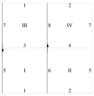
Figure 1: A $2\times 2$ lattice with two Polyakov lines.

The complex density depends now on 8 link angles labeled as in figure1. To save writing we sometimes denote a component by its mere number i.e. $x_{5}\rightarrow 5$

$$\rho(\vec{x})= B(3+8-1-7)B(4+7-2-8)$$

$$B(1+6-3-5)B(2+5-4-6)$$

$$U(-5-7)U(6+8)$$

where

$$B(\phi)=e^{\beta\cos{(\phi)}}\,,U(\phi)=e^{i\phi}$$ (60)

Many link variables are redundant due to the gauge invariance. However in two dimensions one can rewrite the partition function, up to a constant Jacobian, in terms of independent plaquette angles $\vec{\phi}$

$$Z_{\phi}=\int_{\vec{\phi}}\rho(\vec{\phi}).$$ (61)

For a 2x2 lattice there are three independent plaquettes and we choose $(\phi_{I},\phi_{II},\phi_{III})\equiv(\phi_{1},\phi_{2},\phi_{3})$ as our variables

$$\rho(\vec{\phi})=B(\phi_{1})B(\phi_{2})B(\phi_{3})B(\phi_{1}+\phi_{2}+\phi_{3})U(\phi_{1})U(\phi_{3}).$$ (62)

The only reason this system does not factorize is due to the constraint $\phi_{1}+\phi_{2}+\phi_{3}+\phi_{4}=0$, forced by the periodic boundary conditions.

The Fourier components are then

$$a_{\vec{n}}= \int_{-\pi}^{\pi}\frac{d\phi_{1}}{2\pi}e^{-in_{1}\phi_{1}}\int_{-\pi}^{\pi}\frac{d\phi_{2}}{2\pi}e^{-in_{2}\phi_{2}}\int_{-\pi}^{\pi}\frac{d\phi_{3}}{2\pi}e^{-in_{3}\phi_{3}}$$

$$e^{\beta\cos(\phi_{1})}e^{\beta\cos(\phi_{2})}e^{\beta\cos(\phi_{3})}e^{\beta\cos(\phi_{1}+\phi_{2}+\phi_{3})}e^{i(\phi_{1}+\phi_{3})}=$$

$$\sum_{m}I_{m}I_{m-n_{2}}I_{m-n_{1}+1}I_{m-n_{3}+1}$$ (63)

and the corresponding positive density can be readily constructed. Replacing $\phi_{k}$ by $x_{k}+iy_{k}$, we get

$$P(\vec{x},\vec{y})= \frac{a_{\vec{0}}}{2}\left(\delta(\vec{y}-\vec{y}_{s})+\delta(\vec{y}+\vec{y}_{s})\right)$$

$$+ \sum_{\vec{n}\neq\vec{0}}\left\{\frac{e^{\vec{n}\cdot\vec{y}_{s}}a_{\vec{n}}-e^{-\vec{n}\cdot\vec{y}_{s}}a_{-\vec{n}}}{2\sinh{(2\vec{n}\cdot\vec{y}_{s})}}\delta(\vec{y}-\vec{y}_{s})+\frac{e^{\vec{n}\cdot\vec{y}_{s}}a_{-\vec{n}}-e^{-\vec{n}\cdot\vec{y}_{s}}a_{\vec{n}}}{2\sinh{(2\vec{n}\cdot\vec{y}_{s})}}\delta(\vec{y}+\vec{y}_{s})\right\}e^{i\vec{n}\cdot\vec{x}}$$ (64)

To guarantee that zero of sinh is only at the origin, we take $\vec{y}_{s}=y_{s}(1,\sqrt{2},\sqrt{3})$. Again choosing large enough $y_{s}$ makes the lowest mode dominant, leading to positivity of $P$.

Remark: There is a mathematical (number theoretic) subtlety behind this: while it is obvious that the denominator can never vanish, it will nevertheless become very small whenever the integer vector $\vec{n}$ becomes very nearly parallel to a real vector $\vec{y}$ with $\vec{y}\cdot\vec{y}_{s}=0$. Numerically we see that this happens only for $|\vec{n}|$ so large that the decay of the Fourier coefficients $a_{\vec{n}}$ compensates for the small denominator.

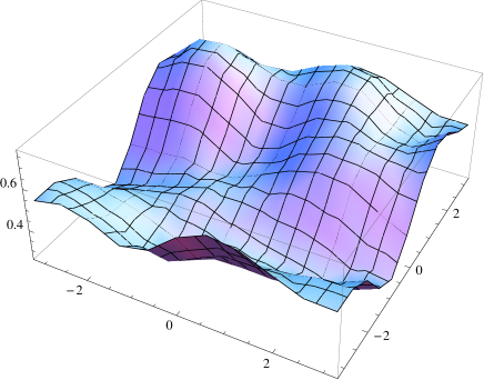
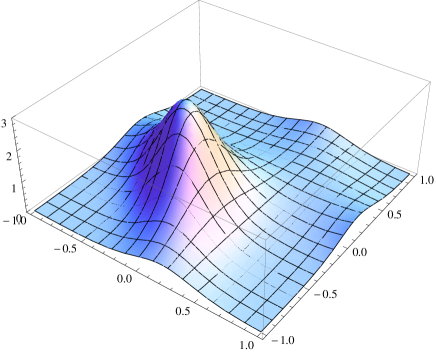
Figure 2: Positive densities with (left) and without the Polyakov loop (right).

A particular cross section $-\pi<x_{1}<\pi,\;-\pi<x_{2}<\pi,\;$of $P^{+}(\vec{x})$ at $x_{3}=.6\pi$ and $y_{s}=8.0$ is displayed in figure 2. To see the effect of Polyakov lines we show also the original positive Boltzmann weight eq.(62) without the loop factors. Needless to say, the effect of Polyakov lines is dramatic, emphasizing the relevance of the statistical formulation.

The second good news is that the variation of $P$ is substantial. This means that the dominance of the first mode, required for positivity, does not preclude the importance of other modes giving rise to a nontrivial structure of the positive distribution.

Instead of checking a particular simple observable, we can verify that the matching equations are satisfied for arbitrary moments of three independent U(1) variables.

It is readily seen that the normalisation of both densities indeed coincide

$$\int\frac{d^{3}\phi}{(2\pi)^{3}}\rho(\vec{\phi})=\int\frac{d^{3}x}{(2\pi)^{3}}d^{3}yP(\vec{x},\vec{y})\equiv Z=a_{\vec{0}}$$ (65)

It remains to verify the averages of generic moments

$$\langle\left(e^{i\phi_{1}}\right)^{r_{1}}\left(e^{i\phi_{2}}\right)^{r_{2}}\left(e^{i\phi_{3}}\right)^{r_{3}}\rangle_{\rho(\vec{\phi})}=\langle\left(e^{i(x_{1}+iy_{1})}\right)^{r_{1}}\left(e^{i(x_{2}+iy_{2})}\right)^{r_{2}}\left(e^{i(x_{3}+iy_{3})}\right)^{r_{3}}\rangle_{P(\vec{x},\vec{y})}$$ (66)

The LHS is obviously the Fourier component $a_{-\vec{r}}$.

On the other hand, the positive distribution $P$ reproduces the Fourier modes by its very construction. Let us check this nevertheless.

$$Z\langle\left(e^{i(x_{1}+iy_{1})}\right)^{r_{1}}\left(e^{i(x_{2}+iy_{2})}\right)^{r_{2}}\left(e^{i(x_{3}+iy_{3})}\right)^{r_{3}}\rangle_{P(\vec{x},\vec{y})}=$$

$$\int d^{3}ye^{-\vec{r}\cdot\vec{y}}\int\frac{d^{3}x}{(2\pi)^{3}}e^{i\vec{r}\cdot\vec{x}}\Biggl{(}\frac{a_{\vec{0}}}{2}\delta(\vec{y}-\vec{y}_{s})+\frac{a_{\vec{0}}}{2}\delta(\vec{y}+\vec{y}_{s})+$$

$$\sum_{\vec{n}\neq\vec{0}}e^{i\vec{n}\cdot\vec{x}}\left\{\frac{e^{\vec{n}\cdot\vec{y}_{s}}a_{\vec{n}}-e^{-\vec{n}\cdot\vec{y}_{s}}a_{-\vec{n}}}{2\sinh{(2\vec{n}\cdot\vec{y}_{s})}}\delta(\vec{y}-\vec{y}_{s})+\frac{e^{\vec{n}\cdot\vec{y}_{s}}a_{-\vec{n}}-e^{-\vec{n}\cdot\vec{y}_{s}}a_{\vec{n}}}{2\sinh{(2\vec{n}\cdot\vec{y}_{s})}}\delta(\vec{y}+\vec{y}_{s})\right\}\Biggr{)}$$

$$a_{\vec{0}}\delta_{\vec{r}}+(1-\delta_{\vec{r}})\left(e^{-\vec{r}\cdot\vec{y}_{s}}\frac{e^{-\vec{r}\cdot\vec{y}_{s}}a_{-\vec{r}}-e^{\vec{r}\cdot\vec{y}_{s}}a_{\vec{r}}}{2\sinh{(-2\vec{r}\cdot\vec{y}_{s})}}+e^{\vec{r}\cdot\vec{y}_{s}}\frac{e^{-\vec{r}\cdot\vec{y}_{s}}a_{\vec{r}}-e^{\vec{r}\cdot\vec{y}_{s}}a_{-\vec{r}}}{2\sinh{(-2\vec{r}\cdot\vec{y}_{s})}}\right)=a_{-\vec{r}}$$

3.4 Larger lattices and separability in plaquette variables

Generalization to larger lattices is straightforward, c.f. figure 3.

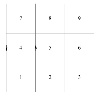
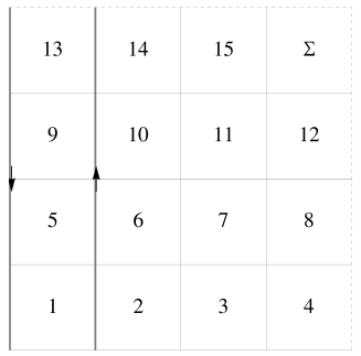
Figure 3: Towards larger abelian lattices. Plaquette labeled Σ $\Sigma$ is determined by the others and periodic boundary conditions.

For example the complex weight which includes two Polyakov lines on the 3x3 periodic lattice reads

$$\rho(1...8)=B(1)B(2)...B(8)B(1+2+3+...+8)U(1)U(4)U(7)$$ (67)

and its Fourier components are readily available

$$a_{\vec{n}}=\sum_{m}(I_{m-n_{7}+1}I_{m-n_{8}}I_{m})\,(I_{m-n_{4}+1}I_{m-n_{5}}I_{m-n_{6}})\,(I_{m-n_{1}+1}I_{m-n_{2}}I_{m-n_{3}})$$ (68)

and similarly for larger, $N\times N$, lattices. The rule for arbitrary lattice is evident: the Fourier coefficients are the sums, over one flux $m$, of products of $N^{2}$ modified Bessel functions. The indices of Bessel functions are given by the differences $m-n_{i}$ if corresponding plaquettes do not tail inner region between the Polyakov lines and they are shifted by one if they do. The index of the last Bessel function is just $m$. All this is well known e.g. from the duality transformations studied decades ago [33, 34].

Corresponding positive distributions follow from our general representation eq.(23).

Before concluding this section let us discuss briefly the issues of locality and separability of resulting positive distributions in the case of many variables.

In practical applications it is desirable, but not necessary, that $P(\vec{x},\vec{y})$ admits a local update algorithm. For example the original density eq.(67) without Polyakov lines does so. Even the ”last” Boltzmann factor can be easily accommodated by a local algorithm. Alternatively one can employ a free boundary conditions or just ignore the single constraint in the large $N$ limit. In this case our complex density reads

$$\rho(\vec{\phi})=\left(\prod_{exterior\;of\;W}B(\phi_{ext})\right)\left(\prod_{interior\;of\;W}B(\phi_{int})U(\phi_{int})\right)$$ (69)

This does not only factorize, but separates as well, i.e. no common variables are shared among these factors. Therefore our construction can be applied independently to each factor.

However in higher dimensions there are many more relations between plaquette variables, even for free boundary conditions, so the positive measures will be highly nonlocal and one has to look for other possibilities.

Second, with more variables the direct Fourier inversion becomes much more time consuming. Hence one should explore other representations which would allow resummation of the series eq.(10).

It remains to be seen to what extent the freedom inherent in the whole approach can be used to circumvent these problems and to generalize the method to more interesting, higher dimensional systems.

4 Summary and directions of future research

Given a complex measure on an $N-$torus, we have presented a general construction of a positive (probability) measure on the complexification of that torus, which is equivalent in the sense that expectations of holomorphic observables agree. We identified necessary and sufficient conditions which such a measure has to fulfill (in addition to being positive) and tested the construction in a number of cases.

Our examples range from one to many degrees of freedom, also with local gauge invariance. They all focus on the classic, by now, question of the space structure of confining strings. It was attracting considerable attention from the beginning of lattice field theory. However the problem was always plagued by strong oscillations of the measure induced by Wilson lines. In the last application the positive density, which incorporates Wilson lines, is explicitly constructed. Even though this is achieved for the simple abelian, and lower dimensional, system the intricacies of the large number of variables were successfully addressed, and exposed in this context, for the first time.

We did not present in this paper an algorithm capable of dealing with complex actions on large lattices. The reason is that the positive measures we are able to construct, are not local in the sense that they are not built up from contributions located at links, plaquettes or other small structures. Our aim was so far to demonstrate mathematically that positive measures representing complex ones exist quite generally, and to provide an explicit construction for them.

With respect to their inherent nonlocality, our measures should be compared to the effective measures for theories with fermions featuring a nonlocal determinant of the Dirac operator (and zero chemical potential). In that case, eventually a workable algorithm was found: the universally used ‘Hybrid Monte Carlo’ algorithm. So one direction of research to be pursued is to search for the possibility to overcome the nonlocality obstacle. Let us list several avenues that could be followed:

1) Search for an analogue of the ‘Hybrid Monte Carlo’ algorithm for our measures.

2) Since the key of the construction is to decompose the complex measure using harmonic (Fourier) analysis, Fast Fourier Transform (FFT) could be helpful.

3) Applying the Real Langevin algorithm to our positive measures appears to be feasible, just as the Complex Langevin algorithm can be applied to full QCD with chemical potential [18, 25]. For toy models the Real Langevin algorithm has been applied successfully, but this is rather trivial and we do not want to burden the reader with details about such a well-known method.

4) Salcedo [30] has devised an ingenious scheme to deal with the nonlocality issue by regarding each variable to be updated separately. The original complex measure, keeping all other variables fixed, is considered as a measure for only the variable to be updated; by complexifying only the variable in question, one obtains an equivalent positive measure for this variable, which can then be updated by a standard Monte Carlo procedure. The feasibility of this strategy for larger lattices is yet to be tested.

Furthermore there is the issue of generalizing the construction to non-abelian gauge theories. A straightforward generalization would use harmonic analysis for non-abelian groups. Some results in this direction have been recently obtained in Ref. [35].

Acknowledgment: this work is supported in part by the NCN grant UMO-2016/21/B/ST2/01492.

References

- [1] K. G. Wilson, Confinement of Quarks, Phys. Rev. D10 (1974) 2445.
- [2] M. Creutz, Monte Carlo Study of Renormalization in Lattice Gauge Theory, Phys. Rev. D23 (1981) 1815.
- [3] Peter Weisz and Pushan Majumdar (2012), Lattice gauge theories, Scholarpedia, 7(4):8615.
- [4] C. Liu, Review on Hadron Spectroscopy, PoS(LATTICE2016)006, arXiv:1612.00103 [hep-lat].
- [5] M. Fukugita, I. Niuya, Distribution of Chromoelectric Flux in SU(2) Lattice Gauge Theory, Phys. Lett. B132 (1983) 374.
- [6] J. Wosiek and R. W. Haymaker,“On the Space Structure of Confining Strings,” Phys. Rev. D 36 (1987) 3297.
- [7] H. Ichie, V. Bornyakov, T. Streuer and G. Schierholz, Flux tubes of two and three quark system in full QCD, Nucl. Phys. A721 (2003) 899.
- [8] F. Karsch, Lattice simulations of the thermodynamics of strongly interacting elementary particles and the exploration of new phases of matter in relativistic heavy ion collisions, J. Phys. Conf. Ser. 46 (2006) 122 [hep-lat/0608003].
- [9] F. A. Berezin, The Method of Second Quantization, Academic Press, N.Y., 1966.
- [10] S. Duane, A. D. Kennedy, B. J. Pendleton and D. Roweth,“Hybrid Monte Carlo,”Phys. Lett. B 195 (1987) 216.
- [11] J. Berges and I.-O. Stamatescu, Simulating nonequilibrium quantum fields with stochastic quantization techniques, Phys. Rev. Lett. 95 (2005) 202003 [hep-lat/0508030].
- [12] J. Berges, S. Borsanyi, D. Sexty and I.-O. Stamatescu, Lattice simulations of real-time quantum fields, Phys. Rev. D75 (2007) 045007 [hep-lat/0609058].
- [13] G. Parisi, On complex probabilities Phys. Lett. B131 (1983) 393.
- [14] J. R. Klauder, Coherent-state Langevin equations for canonical quantum systems with applications to the quantized Hall effect Phys. Rev. A29 (1984) 2036.
- [15] G. Aarts and I. O. Stamatescu, Stochastic quantization at finite chemical potential, JHEP 0809 (2008) 018 [arXiv:0807.1597 [hep-lat]].
- [16] E. Seiler, D. Sexty, I.-O. Stamatescu, Gauge cooling in complex Langevin for QCD with heavy quarks, Phys. Lett. B723 (2013) 213.
- [17] G. Aarts, F. Attanasio, B. Jäger and D. Sexty, The QCD phase diagram in the limit of heavy quarks using complex Langevin dynamics, JHEP 1609 (2016) 087.
- [18] D. Sexty, Simulating full QCD at nonzero density using the complex Langevin equation, Phys. Lett. B729 (2014) 108 [arXiv:1307.7748 [hep-lat]].
- [19] G. Aarts, E. Seiler, D. Sexty and I. O. Stamatescu, Simulating QCD at nonzero baryon density to all orders in the hopping parameter expansion, Phys. Rev. D90 (2014) 114505 [arXiv:1408.3770 [hep-lat]].
- [20] J. Ambjorn and S. -K. Yang, Numerical problems in applying the Langevin equation to complex effective actions, Phys. Lett. B165 (1985) 140.
- [21] R. W. Haymaker and J. Wosiek, Complex Langevin simulations of non-Abelian integrals, Phys. Rev. D37 (1988) 969.
- [22] G. Aarts, F. A. James, E. Seiler, I.-O. Stamatescu, Complex Langevin: Etiology and Diagnostics of its Main Problem, Eur. Phys. J. C71 (2011) 1756.
- [23] J.. Bloch, J. Mahr and S. Schmalzbauer, “Complex Langevin in low-dimensional QCD: the good and the not-so-good,” PoS LATTICE 2015 (2016) 158 [arXiv:1508.05252 [hep-lat]].
- [24] J. Glesaaen, M. Neuman and O. Philipsen, Equation of state for cold and dense heavy QCD, JHEP 1603 (2016) 100 [arXiv:1512.05195[hep-lat]].
- [25] G. Aarts, E. Seiler, D. Sexty and I. O. Stamatescu, Complex Langevin dynamics and zeroes of the fermion determinant, JHEP 1705 (2017) 044 [arXiv:1701.02322 [hep-lat]].
- [26] P. Damgaard and H. Hüffel Stochastic quantization, Phys. Rep. 152 (1987)227.
- [27] D. Weingarten, Complex probabilities on as real probabilities on and application to path integrals, Phys. Rev. Lett. 89 (2002) 240201-1.
- [28] L. L. Salcedo, Representation of complex probabilities, J. Math. Phys. (N.Y.) 38 (1997) 1710.
- [29] L. L. Salcedo, Existence of positive representations for complex weights, J. Phys. A40 (2007) 9399.
- [30] L. L. Salcedo, Gibbs sampling of complex valued distributions, Phys. Rev. D94 (2016) 074503.
- [31] L. L. Salcedo, Does the complex Langevin method give unbiased results?, Phys. Rev. D94 (2016) 114505 [arXiv:1611.06390 [hep-lat]].
- [32] J. Wosiek, Beyond complex Langevin equations: from simple examples to positive representation of Feynman path integrals directly in the Minkowski time, JHEP 1604 (2016) 146 [arXiv:1511.09114 [hep-th]].
- [33] S. Elitzur, R. B. Pearson and J. Shigemitsu, The Phase Structure of Discrete Abelian Spin and Gauge Systems, Phys. Rev. D19 (1979) 3698.
- [34] T. Banks, R. Myerson and J. B. Kogut, Phase Transitions in Abelian Lattice Gauge Theories, Nucl. Phys. B129 (1977) 493.
- [35] L. L. Salcedo, Representation of complex probabilities and complex Gibbs sampling, Proc. of the 35th International Symp. on Lattice Field Theory (Lattice 2017, Granada, Spain) EPJ Web Conf. (arXiv:1710.03195) in press.
- [36] B. Ruba and A. Wyrzykowski, Explicit positive representation for weights on , Proc. of the 35th International Symp. on Lattice Field Theory (Lattice 2017, Granada, Spain) EPJ Web Conf. (arXiv:1710.04318) in press.
- [37] A. Wyrzykowski and B. Ruba, Satisfying positivity conditions in Beyond Complex Langevin approach, Proc. of the 35th International Symp. on Lattice Field Theory (Lattice 2017, Granada, Spain) EPJ Web Conf. (arXiv:1710.04828) in press.