Exploring anomalous $hb\bar{b}$ and $hb\bar{b}\gamma$ couplings in the context of the LHC and an $e^{+}e^{-}$ collider

Abstract

In the light of the 125 GeV Higgs ($h$) discovery at the Large Hadron Collider (LHC), one of the primary goals of the LHC and possible future colliders is to understand its interactions more precisely. Here we have studied the $h$-$b$-$\bar{b}$-$\gamma$ effective interaction terms arising out of gauge invariant dimension six operators in a model independent setting, as a potential source of new physics. Their role in some detectable final states have been compared with those coming from anomalous $h$-$b$-$\bar{b}$ interactions. We have considered the bounds coming from the existing collider and other low energy experimental data in order to derive constraints on the potential new physics couplings and predict possible collider signals for the two different new physics scenarios in the context of 14 TeV LHC and and a future $e^{+}e^{-}$ machine. We conclude that the anomalous $h$-$b$-$\bar{b}$-$\gamma$ coupling can be probed at the LHC at 14 TeV at the 3$\sigma$ level with an integrated luminosity of $\sim 2000~{}{\rm fb}^{-1}$, which an $e^{+}e^{-}$ collider can probe at the 3$\sigma$ level with $\sim 12(7)~{}{\rm fb}^{-1}$ at $\sqrt{s}=250(500)~{}{\rm GeV}$. It is also found that anomalous $h$-$b$-$\bar{b}$ interactions, subject to the existing LHC constraints, can not compete with the rates driven by $h$-$b$-$\bar{b}$-$\gamma$ effective interactions.

I Introduction

The question as to whether the 125 GeV scalar, discovered in 2012 Aad et al. (2012); Chatrchyan et al. (2012), is ‘the Higgs’ or ‘a Higgs’ continues to be pertinent. The second possibility may give us a much-awaited glimpse of physics beyond the standard model. Experimentally, one of the most important endeavors in this respect is to measure carefully the coupling strengths of the scalar to standard model (SM) particle pairs. This has to be backed up with theoretical predictions on the observable consequence of deviation from SM couplings, not only at the Large Hadron Collider (LHC) but also at high-energy $e^{+}e^{-}$ collisions.

A one-stroke pointer to ‘non-standardness’ could of course be the Higgs self-coupling strength which, however, is notoriously difficult to measure precisely, at the LHC as well as in electron-positron machines. The (effective) couplings of the ‘Higgs’ to $W$, $Z$ and photon pairs are being probed with increasing precision, largely because of either the abundance or the distinctiveness of the resulting final states. The measurements related to fermion pair couplings, especially those to $b{\bar{b}}$ and $\tau^{+}\tau^{-}$ pairs, still exhibit considerable uncertainty. For $hb{\bar{b}}$ interaction, in particular, the measurement of total rates of two-body decays (as reflected in the so-called signal strength, namely, $\mu=\sigma/\sigma_{SM}$) remains the only handle, and is beset with a substantial error-bar. The decay kinematics for $h\to b{\bar{b}}$ is difficult to use to one’s benefit. This is because (a) the two-body decay is isotropic in the rest frame of $h$, a spinless particle, and (b) the b-hadrons mostly do not retain information such as that of the polarisation of the b-quark formed. Such information could have potentially revealed useful clues on the Lorentz structure of the $hb{\bar{b}}$ coupling, where a small deviation from the SM nature could be a matter of great interest. This is what stonewalls investigations based on model-independent, gauge-invariant effective couplings, of which exhaustive lists exist in the literature Buchmuller and Wyler (1986); Grzadkowski et al. (2010); Dedes et al. (2017).

Under such circumstances, one line of thinking, where one may be greeted by new physics, is to look not for effective couplings involving the Higgs-like object and a $b{\bar{b}}$-pair, but those which lead to three-body decays of the $h$ rather than a two-body one. We investigate this possibility by considering the $hb{\bar{b}}\gamma$ effective interaction. This interaction should exhibit departure from the SM character as a result of new physics in the sector comprising the $h$ and the bottom quark, contributing to the three-body radiative decay $h\to b{\bar{b}}\gamma$. Here we focus on this kind of Higgs decay. Just like the $hb{\bar{b}}$ effective coupling, the anomalous ‘radiative coupling’, too, can be motivated from dimension-6 gauge invariant effective operators. However, the coefficients of such operators are much less constrained from existing data. This immediately implies possible excess/modification in the signal rate for $pp\to hX\to b\bar{b}\gamma X$. The signal, however, can be mimicked by not only SM channels but also radiative Higgs decays where anomalous $hb{\bar{b}}$ interactions play a part. We show that current constraints allow such values of the effective $hb{\bar{b}}\gamma$ coupling strength, for which the resulting three-body radiative Higgs decays can be distinguished from standard model backgrounds at the LHC as well as high-energy $e^{+}e-$ colliders. Furthermore, they lead to excess $b{\bar{b}}\gamma$ events at a rate which cannot be faked by anomalous $hb{\bar{b}}$ interaction, given the existing constraints on the latter.

The paper is organised in the following way. In section II we discuss the effective Lagrangian terms we have used for our study and the new couplings parameterising the BSM contribution to the Higgs interaction terms. In this section, we also discuss the higher dimensional operators which can give rise to such terms, and show the constraints on the new parameters using Higgs measurement data at the LHC. In section III, we present our collider analyses for the two BSM scenarios (those involving anomalous $hb{\bar{b}}\gamma$ as well as $hb{\bar{b}}$ couplings) we consider here in the context of both the LHC and $e^{+}e^{-}$ colliders. We have also proposed a kinematic variable which can help to distinguish between a two-body and a three-body Higgs decay giving rise to similar final states. We summarise and conclude in section IV.

II Higgs-bottom anomalous coupling

II.1 Parameterization of the interactions

As has already been stated, we adopt a model independent approach, parameterizing the anomalous $hb{\bar{b}}\gamma$ vertex in terms of Wilson coefficients that encapsulate the effects of the high scale theory entering into low-energy physics. Such interaction terms follow from $d>4$, $SU(2)\times U(1)$ gauge-invariant operators. This is consistent with the assumption that their origin lies above the electroweak symmetry breaking scale.

The anomalous interactions relevant for our study are as follows:

• The $h$-$b$-$\bar{b}\gamma$ vertex of the form

  $${\mathcal{L}}_{hb\bar{b}\gamma}=\frac{1}{\Lambda^{2}}F^{\mu\nu}\bar{b}\sigma_{\mu\nu}(d_{1}+id_{2}\gamma_{5})bh$$ (1)

  Such an effective coupling can arise out of dimension 6 operators of the form Grzadkowski et al. (2010); Dedes et al. (2017)

  $$O_{dB}\sim\frac{1}{\Lambda^{2}}(\bar{q}_{p}\sigma^{\mu\nu}d_{r})\Phi B_{\mu\nu}$$ (2)

  and

  $$O_{dW}\sim\frac{1}{\Lambda^{2}}(\bar{q}_{p}\sigma^{\mu\nu}d_{r})\tau^{i}\Phi W^{i}_{\mu\nu}$$ (3)

  where $\Phi$, $q$ and $d$ are the scalar doublet, left-handed quark doublet and right-handed down type quarks respectively, and $B_{\mu\nu}$ and $W_{\mu\nu}$ are the $U(1)$ and $SU(2)_{L}$ field strength tensors respectively. $\Lambda$ is the cut-off scale at which new physics sets in .

• An $h$-$b$-$\bar{b}$ anomalous vertex modifying the SM coupling strength, can be a potential contributor to the process $h\to b\bar{b}\gamma$. The modification to the SM $h$-$b$-$\bar{b}$ coupling may be written as

  $${\mathcal{L}}_{hb\bar{b}}=\Big{(}\frac{gm_{b}}{2m_{W}}\Big{)}\bar{b}(c_{1}+ic_{2}\gamma_{5})bh.$$ (4)

  where $m_{b}$ and $m_{W}$ are the b-quark and W-boson mass respectively. Again, such interactions may be generated from dimension-6 fermion-Higgs operators of the kind Grzadkowski et al. (2010)

  $$O_{d\phi}\sim\frac{C}{\Lambda^{2}}(\Phi^{\dagger}\Phi)(\bar{q}_{p}d_{r}\Phi)+{\rm h.c.}$$ (5)

for a complex $C$. It should be noted that both the sets $\left\{d_{1},d_{2}\right\}$ and $\left\{c_{1},c_{2}\right\}$ include the possibility of CP-violation, a possibility that cannot be ruled out in view of observations such as the baryon-antibaryon asymmetry in our universe. Thus both of the paired parameters in each case should affect event rates at colliders, irrespectively of whether CP-violating effects can be discerned.

Note that only the contribution from the third family in Eqs. 2, 3 and 5 have been included in the present study. While all possible higher-dimensional operators are in principle to be included in an effective field theory approach, the proliferation of terms (and free parameters) caused by such universal inclusion will make any phenomenological study difficult. Keeping in mind and remembering that our purpose here is to look for non-standard Higgs signals based on $b$-quark interactions, we have assumed that only the terms with $p$=$r$=3 are non-vanishing in Eqs. 2, 3 and 5.

Fig. 1 illustrates how the anomalous couplings affect the three-body decay of the Higgs boson into $b\bar{b}\gamma$ in the two scenarios described above. As has been mentioned in the introduction, our interest is primarily on the first set of anomalous operators, as they have not yet been investigated. However, any observable effect arising from them can in principle be always faked by interactions of the second kind, and therefore the latter need to be treated with due merit in the study of the final states of our interest.

Figure 1: $h\to b\bar{b}\gamma$ via anomalous couplings $h$-$b$-$\bar{b}$ and $h$-$b$-$\bar{b}$-$\gamma$.

II.2 Constraints from Higgs data and other sources

The addition of a non-standard Higgs vertex or having the standard interaction terms with modified coefficients will change the Higgs signal strengths ($\mu=\sigma/\sigma_{SM}$). The Higgs-related data at the LHC already put strong constraints on such deviations, the measured values of $\mu$ being always consistent with unity at the 2$\sigma$-level. The non-standard effects under consideration here will have to be consistent with such constraints to start with. In applying these constraints, we have taken the most updated measurements of various $\mu$-values provided by ATLAS and CMS so far Aad et al. (2014); Khachatryan et al. (2014); Aad et al. (2015a); Chatrchyan et al. (2014a); Aad et al. (2015b, c); Chatrchyan et al. (2014b); Aad et al. (2015d); Chatrchyan et al. (2014c); Aad et al. (2015e); Chatrchyan et al. (2014d); CMS (2015). These values and their corresponding 1$\sigma$ error bars, based on the (7+8) TeV data, are shown in Table 1.

Decay channel	ATLAS+CMS
$\mu^{\gamma\gamma}$	$1.16^{+0.20}_{-0.18}$ Aad et al. (2014); Khachatryan et al. (2014)
$\mu^{ZZ}$	$1.31^{+0.27}_{-0.24}$ Aad et al. (2015a); Chatrchyan et al. (2014a)
$\mu^{WW}$	$1.11^{+0.18}_{-0.17}$ Aad et al. (2015b, c); Chatrchyan et al. (2014b)
$\mu^{bb}$	$1.12^{+0.25}_{-0.23}$ Aad et al. (2015d); Chatrchyan et al. (2014c)
$\mu^{\tau\tau}$	$0.69^{+0.29}_{-0.27}$ Aad et al. (2015e); Chatrchyan et al. (2014d)

Table 1: ATLAS and CMS $\sqrt{s}$=7 and 8 TeV combined $\mu$ values along with their total uncertainties for different Higgs boson decay channels as quoted in Table 11 of Ref. CMS (2015).

The non-standard effective interaction terms in Eq. 1 and 4 have been added to the existing SM Lagrangian using FeynRules Christensen and Duhr (2009); Alloul et al. (2014) modifying the CP-even coupling coefficient in the $h$-$b$-$\bar{b}$ vertex in the latter case to $(1+c_{1})\frac{gm_{b}}{2m_{W}}$.

First consider the effective $h$-$b$-$\bar{b}$-$\gamma$ vertex scenario. This vertex does not contribute to any of the standard Higgs decay modes and gives rise to the three-body decay $h\to b{\bar{b}}\gamma$. This invites an additional perturbative suppression by $\alpha_{em}$ within the framework of the SM, and also in presence of the anomalous couplings $\{c_{1},c_{2}\}$. However, the dimension-6 operators shown in Eq. 2 and 3 can in principle boost this decay channel, depending on the values of $d_{1}$ and $d_{2}$. To the best of our understanding, no dedicated search for $h\to b{\bar{b}}\gamma$ has been reported so far. We therefore depend on global fits of the LHC data which yield an upper limit of about 23$\%$ Aad et al. (2015f) on any non-standard decay branching ratio (BR) of the 125 GeV scalar at 95$\%$ confidence level. This includes, for example, invisible decays as well as decays into light-quark or gluon jets. In our case, the same limit is assumed to apply on BR($h\to b\bar{b}\gamma$), which translates into a bound on the couplings $|d_{1}|,|d_{2}|\leq$ 10 for $d_{1}\approx d_{2}$. However, such a large BR for $h\to b\bar{b}\gamma$ might affect the event count for a $h\to b\bar{b}$ study if the photon goes untagged. Also, it might come into conflict with the predicted two-gluon BR for the Higgs, if the invisible decay width gets further constrained by even a small amount. In view of this, we have carried out our analysis with a relatively conservative choice, namely, $|d_{1}|,|d_{2}|\leq$ 5. It is found that, even with such values, the contribution to BR($h\to b\bar{b}\gamma$) is about one order higher than what could come from purely SM interactions. Thus the effects of such additional couplings are unlikely to be faked by SM effects. The new physics parameters $d_{1}$ and $d_{2}$ are not constrained from any other experimentally measured quantities. In principle, $d_{2}$ could be constrained from neutron electric dipole moment (nEDM) measurement Pospelov and Ritz (2005); Baker et al. (2006); Czarnecki and Krause (1997); Brod et al. (2013) since the presence of the $h$-$b$-$\bar{b}$-$\gamma$ vertex can lead to contribution to the up quark EDM at one-loop level as shown in Fig. 2.

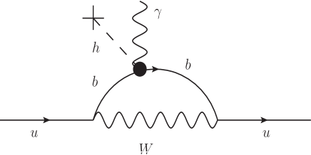
Figure 2: Contribution to the up-quark EDM arising from the anomalous $h$-$b$-$\bar{b}$-$\gamma$ vertex at one loop.

The contribution to the up quark EDM ($d_{u}$) coming from this anomalous vertex is given as

$$\frac{d_{u}}{e}\simeq\frac{d_{2}}{3}\frac{m_{u}m_{b}}{{m_{W}}^{2}-{m_{b}}^{2}}\left(\frac{|V_{ub}|g}{2\sqrt{2}}\right)^{2}\left(\frac{v}{\Lambda^{2}}\right)K(\Lambda,m_{W},m_{b})$$ (6)

where $K(\Lambda,m_{W},m_{b})=\frac{1}{4\pi^{2}}\Big{[}\frac{5}{8}+\frac{3}{4}{\rm ln}(\frac{\Lambda^{2}}{{m_{W}}^{2}})-{\rm ln}(\frac{\Lambda^{2}}{{m_{b}}^{2}})\Big{]}$.
Here $m_{u}$ is the up quark mass, $m_{W}$ is the mass of W boson, $m_{b}$ is the $b$-quark mass and $v$ is the Higgs vacuum expectation value respectively. As is evident from Eq. 6, the contribution to nEDM from such a diagram is proportional to the quark mixing element, $|V_{ub}|^{2}$. The smallness of $|V_{ub}|(\sim 4\times 10^{-3})$ results in a suppressed nEDM contribution and thus the constraint on $d_{2}$ becomes much more relaxed compared to that derived from non-standard Higgs decay branching ratio constraint.

The situation is different for the anomalous effective $hb\bar{b}$ vertex scenario. Since this vertex directly affects the most dominant Higgs decay mode, i.e $h\to b\bar{b}$, the existing Higgs data impose a much more severe constraint on the non-standard couplings in this case, since even a small change in the BR($h\to b\bar{b}$) can alter the other SM Higgs signal strengths significantly. In order to ascertain the consequently allowed values of $\{c_{1},c_{2}\}$, we compute the corresponding $\mu$-values within our effective theory framework. Non-vanishing $c_{1},c_{2}$ are assumed to keep the Higgs production rate unaffected, and all other Higgs couplings are assumed to be SM-like for simplicity of the analysis. The allowed regions thus obtained at the 95.6% C.L. are shown in Fig. 3.

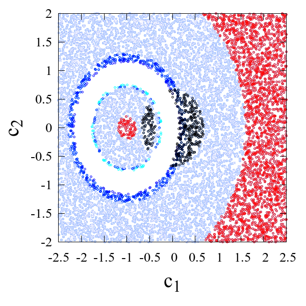
Figure 3: The light blue, red, blue, cyan and black points indicate the regions of the parameter space excluded from the signal strength ($\mu$) measurements of $\tau\bar{\tau}$, $b\bar{b}$, $\gamma\gamma$, $WW^{*}$ and $ZZ^{*}$ decay modes of the Higgs at 2$\sigma$ level. The blank space is the allowed region.

The white annular region in Fig. 3 represents the allowed 95.6% C.L. parameter space in the $c_{1}$-$c_{2}$ plane. The light blue, red, blue, cyan and black regions are excluded by the measurement of $\mu^{\tau\tau}$, $\mu^{bb}$, $\mu^{\gamma\gamma}$, $\mu^{WW}$ and $\mu^{ZZ}$ respectively. Note that large positive values of $c_{1}$ will be disfavored since it tends to enhance BR($h\to b\bar{b}$) beyond acceptable limits.

III Collider Analysis

Collider signatures of possible anomalous Higgs vertices have been studied both theoretically, see e.g. Gonzalez-Garcia (1999); Han and Jiang (2001); Choi et al. (2003); Han and Mellado (2010); Gao et al. (2010); De Rujula et al. (2010); Desai et al. (2011); Boughezal et al. (2012); Stolarski and Vega-Morales (2012); Djouadi et al. (2013); Godbole et al. (2014); Banerjee et al. (2012, 2014); Gunion and He (1996); Chen et al. (2014); Han et al. (2015); Boudjema et al. (2015); Braguta et al. (2003a); Hagiwara et al. (2016); Dwivedi et al. (2016), and experimentally Aad et al. (2016); Khachatryan et al. (2016). However, as has been already stated, none of these studies include three-body decays such as $h\to b\bar{b}\gamma$ and their possible signals at colliders.

Keeping collinear divergences in mind, we have retained the b-quark mass. In addition, we make sure that the photon is well-separated from the $b$-partons at the generation level. The non-standard effective Lagrangian terms have been encoded using FeynRules in order to generate the model files for implementation in MadGraph Alwall et al. (2011, 2014) which was used for computing the required cross-sections and generating events for collider analyses. The Higgs branching ratios are calculated at the tree-level.

We have put a minimum isolation, namely, $\Delta R>0.4$, between any two visible particles in the final state while generating the events at the parton level. Additionally, we have put minimum $p_{T}$ thresholds on both the $b$-jets and the photon, namely, $p_{T}^{b}>20$ GeV and $p_{T}^{\gamma,\ell}>10$ GeV. These cuts ensure that a certain angular separation is maintained among the final state particles, thus avoiding the infrared and collinear divergences in the lowest order calculation. For the effective $h$-$b$-$\bar{b}$-$\gamma$ scenario, MadGraph treats $h\to b\bar{b}\gamma$ as just another non-standard decay of the Higgs at the tree level. However, for the effective $h$-$b$-$\bar{b}$ scenario, the $\gamma$ has to be radiated from one of the $b$-partons originating from $h$. The cancellation of the already mentioned infrared/collinear divergences in such a case calls for a full one-loop calculation. We have checked using MadGraph that the one-loop corrected Higgs decay width in the framework of the SM differs from that at the leading order by a factor of $\sim 1.1$. Hence with such loop-corrected Higgs decay width the relevant branching ratio ($\approx 10^{-4}$) does not differ by more than 1-2$\%$. We have thus retained the tree-level branching ratio for $h\to b\bar{b}\gamma$.

After generating events with MadGraph, we have used PYTHIA Sjostrand et al. (2006) for the subsequent decay, showering and hadronization of the parton level events. For the LHC analysis we have used the nn23lo1 Ball et al. (2015) parton distribution function and the default dynamic renormalisation and factorisation scales http://cp3.irmp.ucl.ac.be/projects/madgraph/wiki/FAQ-General-13 in MadGraph for our analysis. Finally, detector simulation was done using Delphes3 de Favereau et al. (2014). The $b$-tagging efficiency and mistagging efficiencies of the light jets as $b$-jets incorporated in Delphes3 can be found in ATL (2015); Chatrchyan et al. (2013). Jets were constructed using the anti-kT algorithm Cacciari et al. (2008). The following cuts were applied on the jets, leptons and photons at the parton level in Madgraph while generating all the events throughout this work:

• All the charged leptons and jets including $b$-jets are selected with a minimum transverse momentum cut of 20 GeV, $p_{T}^{b,\ell}>20$ GeV. They must also lie within the pseudo-rapidity window $|\eta|^{b,\ell}<2.5$. For $e^{+}e^{-}$ collider analysis, the lepton $p_{T}$ requirement is changed to $p_{T}^{\ell}>10$ GeV following Abramowicz et al. (2013).

• All the photons in the final state must satisfy $p_{T}^{\gamma}>10$ GeV and $|\eta|^{\gamma}<2.5$.

• In order to make sure that all the final state particles are well-separated, we demand $\Delta R>0.4$ between all possible pairs.

Note that we have tagged the hardest photon in the final state in order to reconstruct the 125 GeV Higgs mass. In the signal process we always obtain one such hard photon arising from Higgs decay. However, for the background processes, events can be found with an isolated bremsstrahlung photon or one coming from $\pi^{0}$ decay. In general, photons from showering as well as initial state radiation do constitute backgrounds to our signal, and the selection cuts need to be chosen so as to suppress them.

III.1 Effective $h$-$b$-$\bar{b}$-$\gamma$ scenario

III.1.1 LHC Search

To start with, we are concerned with $b\bar{b}$-pairs (along with a photon) being produced in Higgs decay. Existing studies indicate that, in such a case, $Z$-boson associated production, with $Z$ decaying into an opposite-sign same-flavor lepton pair, is the most suitable one for studying such final states Aad et al. (2015d). We thus concentrate on

$$pp\rightarrow Zh,h\rightarrow b\bar{b}\gamma,Z\rightarrow\ell^{+}\ell^{-}$$ (7)

leading to the final state $\ell^{+}\ell^{-}b\bar{b}\gamma$, with $\ell=e,\mu$. One can also look for associated $Wh$ production where $W$ decays leptonically to yield the $\ell+b\bar{b}\gamma$ final state ($\ell=e,\mu$). However, the signal acceptance efficiency is smaller compared to that for the $Z$-associated production channel Aad et al. (2015d), where the invariant mass of the lepton-pair from Z-decay can be used to one’s advantage. Higgs production via vector boson fusion (VBF) can be another possibility which, however, is more effective in probing gauge-Higgs anomalous vertex Plehn et al. (2002); Hankele et al. (2006). Higgs production associated with a top-pair has a much smaller cross-section https://twiki.cern.ch/twiki/bin/view/LHCPhysics/HiggsEuropeanStrategy and hence is not effective for such studies. Finally, the most dominant Higgs production mode at the LHC, namely, gluon fusion, can give rise to a $b\bar{b}\gamma$ final state which is swamped by the huge SM background.

The main contribution to the SM background comes from the following channels:

1. $pp\rightarrow Zh\gamma,h\rightarrow b\bar{b}$, $Z\rightarrow\ell^{+}\ell^{-}$

2. $pp\rightarrow t\bar{t}\gamma$, $t\rightarrow bW^{-}$, $W^{-}\rightarrow\ell^{-}\nu$

3. $pp\rightarrow\ell^{+}\ell^{-}b\bar{b}\gamma$

4. $pp\rightarrow\ell^{+}\ell^{-}jj\gamma$

Let us re-iterate that the radiative process can in each case be faked by the corresponding process without the photon emission but with the photon arising through showering. Such showering photons, however, are mostly softer than what is expected of the signal photons, since the latter come from three-body decays of the 125 GeV scalar, and thus their $p_{T}$ peaks at values close to 40 GeV.

We use the following criteria (C0) for the pre-selection of our final state:

• The number of jets in the final state: $N_{j}\geq 2$.

• At least one, and not more than two $b$-jets: $1\leq N_{b}\leq 2$.

• One hard photon with $E_{T}\geq 20$ GeV.

• Two same-flavor, opposite-sign charged leptons ($e,\mu$).

Such final states are further subjected to the following kinematical criteria:

• C1: $\cancel{E}_{T}<30$ GeV.

• C2: An invariant mass window for the invariant mass $M_{b\bar{b}(j)\gamma}$ (see Fig. 4): $105~{}{\rm GeV}\leq M_{b\bar{b}(j)\gamma}\leq 135~{}{\rm GeV}$. When two b-jets are tagged, both are included. When only one $b$ is identified, it is combined with the hardest of the remaining jets together with the hardest photon.

  

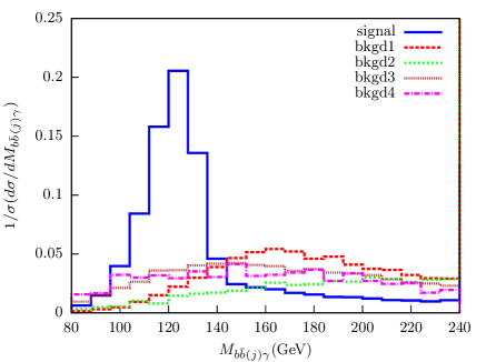
  Figure 4: Normalized distribution for $M_{b\bar{b}(j)\gamma}$ for the signal process ($d_{1}=5.0$, $d_{2}=5.0$) and various background channels : "bkgd1" refers to $pp\rightarrow Zh\gamma$ , "bkgd2" to $pp\rightarrow t\bar{t}\gamma$, "bkgd3" to $pp\to\ell^{+}\ell^{-}b\bar{b}\gamma$ and "bkgd4" to $pp\to\ell^{+}\ell^{-}jj\gamma$ respectively.

• C3: An invariant mass window for the associated lepton pair: $(m_{Z}-15~{}{\rm GeV})\leq M_{\ell^{+}\ell^{-}}\leq(m_{Z}+15~{}{\rm GeV})$.

• C4: Finally, the $Z$ and $h$ are produced almost back-to-back in the transverse plane for our signal process. This, along with the fact that the Higgs decay products are considerably boosted in the direction of the Higgs, prompts us to impose an azimuthal angle cut between the photon and the dilepton system ( Fig. 5): $\Delta\phi(\gamma,\ell^{+}\ell^{-})>1.5$.

  

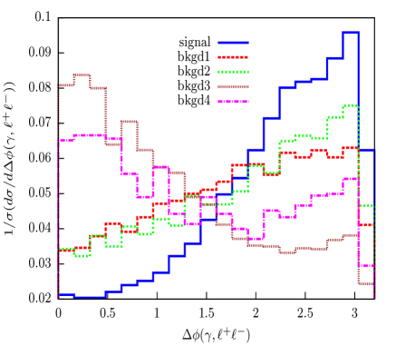
  Figure 5: Normalized distribution for $\Delta\phi(\gamma,\ell^{+}\ell^{-})$ for the signal process ($d_{1}=5.0$, $d_{2}=5.0$) and various background channels : “bkgd1“ refers to $pp\rightarrow Zh\gamma$ , "bkgd2" to $pp\rightarrow t\bar{t}\gamma$, "bkgd3" to $pp\to\ell^{+}\ell^{-}b\bar{b}\gamma$ and "bkgd4" to $pp\to\ell^{+}\ell^{-}jj\gamma$ respectively.

Among the selection criteria listed above, we have checked that C2 and C4 are effective in reducing the contamination from showering photons.

We present the results of our analysis for $\sqrt{s}=14$ TeV. Signal events were generated for $d_{1}=d_{2}=5.0$ which results in BR($h\to b\bar{b}\gamma$)$\simeq 5\%$.

Tables 2 and 3 show the signal rates and the response of signal and background events to the cuts mentioned above.

Process	$\sqrt{s}=$8 TeV	$\sqrt{s}=$14 TeV
	$\sigma$ (pb)	$\sigma$(pb)
$pp\rightarrow Zh,h\to b\bar{b}\gamma$	$1.795\times 10^{-4}$	$3.332\times 10^{-4}$

Table 2: Cross sections at LHC for our signal processes at $\sqrt{s}=$8 TeV and 14 TeV.

Since the production cross-section is small to start with, one depends on the high luminosity run of the LHC. As seen from Table 2, the 8 TeV run has understandably been inadequate to reveal the signal under investigation. Hence any hope of seeing the signal events lies in the high-energy run (14 TeV). A detailed cut-flow table for both the signal and background events is shown in Table 3.

Process	$\sqrt{s}=$14 TeV
	$\sigma$ (pb)	NEV ($\mathcal{L}=$1000 ${\rm fb}^{-1}$)
		C0	C1	C2	C3	C4
$pp\rightarrow Zh,h\to b\bar{b}\gamma$	$3.332\times 10^{-4}$	83	70	41	39	29
$pp\rightarrow Zh\gamma$	$4.765\times 10^{-5}$	17	13	1	1	-
$pp\rightarrow t\bar{t}\gamma$	0.03144	5214	586	31	5	4
$pp\rightarrow\ell^{+}\ell^{-}b\bar{b}\gamma$	0.01373	3149	2507	345	98	54
$pp\rightarrow\ell^{+}\ell^{-}jj\gamma$	3.589	5355	4523	427	213	107

Table 3: Cross-sections for the signal (corresponding to $d_{1}=d_{2}=5.0$) and various background channels are shown in pb alongside the number of expected events for the individual channels at 1000 ${\rm fb}^{-1}$ luminosity after each of the cuts C0-C4 as listed in the text. NEV $\equiv$ number of events.

As we can see, contributions to the background from $pp\to Zh\gamma$ is reduced by the cuts rather significantly, whereas $pp\to\ell^{+}\ell^{-}jj\gamma$ contributes the most. Demanding two $b$-tagged jets in the final state would have significantly reduced this background, given the faking probability of a light jet as a $b$-jet (as emerging from DELPHES). However, that would have reduced our signal events further, since the second hardest b-jet peaks around 30 GeV, and thus the tagging efficiency drops. The next largest contributor to the background events is the process $pp\to\ell^{+}\ell^{-}b\bar{b}\gamma$. The invariant mass and $\Delta\phi$ cuts play rather important roles in reducing both this background and the one discussed in the previous paragraph. The $t{\bar{t}}\gamma$ production channel, too, could contribute menacingly to the background. However, the large missing transverse energy associated with this channel allows us to suppress its effects, by requiring $\cancel{E}_{T}<30$ GeV. Further enhancement of the signal significance occurs via invariant mass cuts on the $b\bar{b}\gamma$ and $\ell^{+}\ell^{-}$ systems. In principle, one may also expect some significant contribution to the background from the production channels $t\bar{t}W^{\pm}\gamma$ and $W^{+}W^{-}\gamma+{\rm jets}$. However, these channels are associated with large $\cancel{E}_{T}$. We have checked that the our $\cancel{E}_{T}$ and $M_{b\bar{b}(j)\gamma}$ requirements render these background contributions negligible. On the whole, the background contributions add up to a total of 165 events compared to 29 signal events at 1000 ${\rm fb}^{-1}$ for our choice of $d_{1}=d_{2}=5.0$, which amounts to a statistical significance of 2.2$\sigma$ for the $\ell^{+}\ell^{-}b\bar{b}\gamma$ final state. Hence a 3$\sigma$ statistical significance can be achieved for such a signal at 14 TeV with a luminosity$\sim$ 1900 ${\rm fb}^{-1}$. Such, and higher, luminosities should be able to probe the signature of the the $hb{\bar{b}}\gamma$ effective interaction with strength well within the present experimental limits.

III.1.2 Search at an $e^{+}e^{-}$ collider

It is evident from the previous section that the scenario under consideration can be probed at least with moderate statistical significance at the LHC at high luminosity at the 14 TeV run. We next address the question as to whether an electron-positron collider can improve the reach.

An $e^{+}e^{-}$ machine is expected to provide a much cleaner environment compared to the LHC. Here the dominant Higgs production modes are the $Z$-boson mediated s-channel process and gauge boson fusion processes, resulting in the production of $Zh$ and $h\nu\bar{\nu}$ respectively Arbey et al. (2015). The $Zh$ mode has the largest cross-section at relatively lower center-of-mass energies ($\sqrt{s}$), peaking around $\sqrt{s}=250$ GeV. However, as $\sqrt{s}$ increases, this cross-section goes down, making this channel less significant while the $W$-boson fusion production mode dominates. Hence we include both these production modes in our analysis and explore our scenario at two different center-of-mass energies, namely, $\sqrt{s}=250$ GeV and 500 GeV. For $\sqrt{s}=250$ GeV, we consider two possible final states depending on whether $Z$ decays into a pair of leptons or a pair of neutrinos. For the latter final state, there is also some contribution from the $W$-fusion diagram, which is small but not entirely negligible. For $\sqrt{s}=500$ GeV, however, most of the contribution comes from the $h\nu\bar{\nu}$ production via $W$ fusion along with a small contribution from $Zh$ production. The production channels we consider are therefore

$$e^{+}e^{-}\rightarrow Zh,Z\rightarrow\ell^{+}\ell^{-},h\rightarrow b\bar{b}\gamma$$ (8)

$$e^{+}e^{-}\rightarrow\nu\bar{\nu}h,h\rightarrow b\bar{b}\gamma$$ (9)

resulting in the final state $\ell^{+}\ell^{-}b\bar{b}\gamma$ or $b\bar{b}\gamma+\cancel{E}$. Let us first take up the $\ell^{+}\ell^{-}b\bar{b}\gamma$ final state, which is relevant for $\sqrt{s}=250$ GeV. The major SM background contributions are:

1. $e^{+}e^{-}\rightarrow Zh\gamma,Z\rightarrow\ell^{+}\ell^{-},h\rightarrow b\bar{b}$

2. $e^{+}e^{-}\rightarrow\ell^{+}\ell^{-}b\bar{b}\gamma$

3. $e^{+}e^{-}\rightarrow\ell^{+}\ell^{-}jj\gamma$. with at least one $j$ faking a $b$-jet.

After passing through the pre-selection cuts C0, the signal as well as the background events are further subjected to the following kinematical requirements:

• D1 : Since we have two same-flavor opposite-sign leptons in the event arising from $Z$-decay, their momentum information can be used to reconstruct the Higgs boson mass irrespective of its decay products via the recoil mass variable defined as

  $$m_{rec}\equiv\sqrt{(\sqrt{s}-E_{\ell^{+}\ell^{-}})^{2}-\vec{p}_{\ell^{+}\ell^{-}}^{2}}$$ (10)

  where $E_{\ell^{+}\ell^{-}}$ and $\vec{p}_{\ell^{+}\ell^{-}}$ are the net energy and three-momentum of the $\ell^{+}\ell^{-}$ system or that of the reconstructed $Z$-boson. This variable is free from jet tagging and smearing effects and shows a much sharper peak at the Higgs mass ($m_{h}$) compared to $M_{b\bar{b}(j)\gamma}$ as shown in Fig. 6. This variable is thus more effective in reducing the SM background. We demand $122~{}{\rm GeV}\leq m_{rec}\leq 128~{}{\rm GeV}$.

  

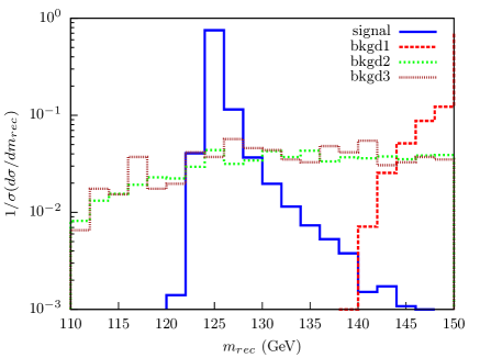
  Figure 6: Normalized distribution for $m_{rec}$ for the signal process ($d_{1}=5.0$, $d_{2}=5.0$) and the backgrounds at $\sqrt{s}=250$ GeV. “bkgd1” refers to $e^{+}e^{-}\rightarrow Zh\gamma,Z\rightarrow\ell^{+}\ell^{-},h\rightarrow b\bar{b}$, “bkgd2” to $e^{+}e^{-}\rightarrow\ell^{+}\ell^{-}b\bar{b}\gamma$ and “bkgd3” to $e^{+}e^{-}\rightarrow\ell^{+}\ell^{-}jj\gamma$ respectively.

• D2 : As before, we select an invariant mass window for the associated lepton pair: $(m_{Z}-15~{}{\rm GeV})\leq M_{\ell^{+}\ell^{-}}\leq(m_{Z}+15~{}{\rm GeV})$.

We summarise our results for our signal and background analysis in the subsequent Tables 4 and 5. As evident from Table 5, variable $m_{rec}$ is highly effective in reducing the background events resulting in a statistical significance of 3$\sigma$ and 5$\sigma$ at $\sim 85~{}\mbox{${\rm fb}^{-1}$}$ and $\sim 250~{}\mbox{${\rm fb}^{-1}$}$ integrated luminosities respectively.

Process	$\sqrt{s}=$250 GeV
	$\sigma$ (pb)
$e^{+}e^{-}\rightarrow Zh,Z\rightarrow\ell^{+}\ell^{-},h\rightarrow b\bar{b}\gamma$	$2.79\times 10^{-4}$

Table 4: Cross-section for the signal process ($d_{1}=5.0$, $d_{2}=5.0$) presented at $\sqrt{s}=250$ GeV, before applying the cuts C0, D1 and D2.

	$\sqrt{s}=$250 GeV
Process	$\sigma$ (fb)	NEV ($\mathcal{L}=$250 ${\rm fb}^{-1}$)
		C0	D1	D2
$e^{+}e^{-}\rightarrow Zh$	0.279	13	11	11
$Z\to\ell^{+}\ell^{-}$, $h\rightarrow b\bar{b}\gamma$
$e^{+}e^{-}\rightarrow Zh\gamma$	0.079	1	-	-
$Z\to\ell^{+}\ell^{-}$, $h\rightarrow b\bar{b}$
$e^{+}e^{-}\rightarrow\ell^{+}\ell^{-}b\bar{b}\gamma$	0.990	19	3	1
$e^{+}e^{-}\rightarrow\ell^{+}\ell^{-}jj\gamma$	3.059	8	1	1

Table 5: Cross-section and expected number of events at 250 ${\rm fb}^{-1}$ luminosity for the signal and various processes contributing to background at $\sqrt{s}=250$ GeV . We have used $d_{1}=d_{2}$ = 5.0, with $\Lambda=1$ TeV.

Although the $\ell^{+}\ell^{-}b\bar{b}\gamma$ final state is capable of probing the $d_{1}$, $d_{2}$ couplings at a reasonable luminosity, it is at the same time interesting to explore the invisible decay of the $Z$, which has a three times larger branching ratio than that of $Z\to\ell^{+}\ell^{-}$. In addition, the $\nu\bar{\nu}b\bar{b}\gamma$ final state can get contribution from the $W$-fusion process as mentioned earlier. This additional contribution becomes dominant at higher center-of-mass energies ($\sqrt{s}\gtrsim 500$ GeV) and hence for this analysis, we present our results for $\sqrt{s}=250$ GeV and 500 GeV. The major SM backgrounds to this final state are as follows:

1. $e^{+}e^{-}\rightarrow\nu\bar{\nu}h\gamma,~{}h\rightarrow b\bar{b}$

2. $e^{+}e^{-}\rightarrow\nu\bar{\nu}b\bar{b}\gamma$

3. $e^{+}e^{-}\rightarrow\nu\bar{\nu}jj\gamma$. with one $j$ faking a $b$-jet.

4. $e^{+}e^{-}\rightarrow t\bar{t}$, $t\rightarrow bW^{-}$, $W^{-}\rightarrow\ell^{-}\nu$

We use the following criteria (I0) to pre-select our signal events:

• We impose veto on any charged lepton with energy greater than 20 GeV.

• Since we are working in a leptonic environment, the presence of ISR jets is unlikely. Hence we restrict the number of jets in the final state, demanding $N_{j}=2$.

• Taking into account the $b$-jet tagging efficiency, as before, we demand $1\leq N_{b}\leq 2$.

• We restrict number of hard photons in the final state: $N_{\gamma}=1$.

Further, the following kinematic selections are made to reduce the SM background contributions:

• I1: Given the fact that the signal has direct source of missing energy ($\cancel{E}$), and that one can measure the net amount of $\cancel{E}$ at an $e^{+}e^{-}$ collider, we demand $\cancel{E}>110$ GeV for $\sqrt{s}=250$ GeV and $\cancel{E}>280$ GeV for $\sqrt{s}=500$ GeV. For illustration, in Fig. 7 we have shown the $\cancel{E}$ distribution for both the signal and background events at $\sqrt{s}=500$ GeV.

  

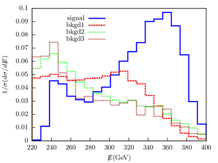
  Figure 7: Normalized distribution for $\cancel{E}$ for the signal process and the backgrounds at $\sqrt{s}=500$ GeV. “bkgd1” refers to $e^{+}e^{-}\rightarrow\nu\bar{\nu}h\gamma,h\rightarrow b\bar{b}$, “bkgd2” to $e^{+}e^{-}\rightarrow\nu\bar{\nu}b\bar{b}\gamma$ and “bkgd3” to $e^{+}e^{-}\rightarrow\nu\bar{\nu}jj\gamma$ respectively.

• I2: Invariant mass reconstructed with the two hardest jets after ensuring that at least one of them is a $b$-jet, and the sole photon in the event should lie within the window (see Fig. 8): $90~{}{\rm GeV}\leq M_{b\bar{b}(j)\gamma}\leq 126~{}{\rm GeV}$.

  

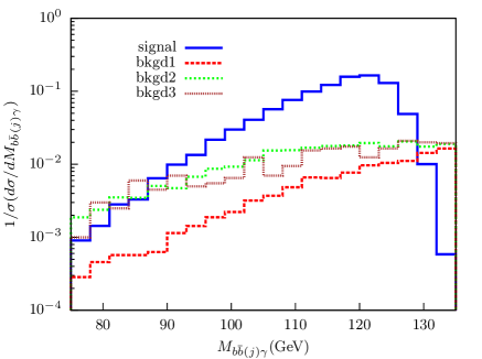
  Figure 8: Normalized distribution for $M_{b\bar{b}(j)\gamma}$ for the signal process and the backgrounds at $\sqrt{s}=500$ GeV.

• I3: Moreover, the invariant mass of the jet pair with $1\leq N_{b}\leq 2$ should lie within the window (see Fig. 9): $20~{}{\rm GeV}\leq M_{b\bar{b}(j)}\leq 70~{}{\rm GeV}$.

  

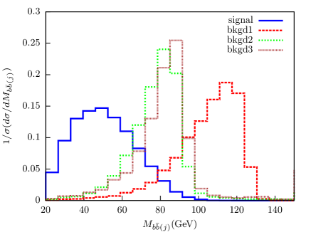
  Figure 9: Normalized distribution for $M_{b\bar{b}(j)}$ for the signal process and the backgrounds at $\sqrt{s}=500$ GeV.

Note that the charged lepton veto as well as the restriction on the number of jets together with the demand of a photon in the final state suppress the $t\bar{t}$ background. In addition I1, I2 and I3 turn out to be quite effective in killing the background. Once more the inclusion of I2 plays an effective role in reducing the contribution from showring photons.

We summarise the results of our analysis in Tables 6 and 7.

Process	$\sqrt{s}=$250 GeV	$\sqrt{s}=$500 GeV
	$\sigma$ (fb)	$\sigma$ (fb)
$e^{+}e^{-}\rightarrow Zh,Z\rightarrow\nu\bar{\nu},h\rightarrow b\bar{b}\gamma$	0.997	0.261
$W$-fusion: $e^{+}e^{-}\rightarrow\nu\bar{\nu}h,h\rightarrow b\bar{b}\gamma$	0.169	1.618

Table 6: Individual cross-sections of the contributing production channels for the signal process $e^{+}e^{-}\rightarrow\nu\bar{\nu}h,h\rightarrow b\bar{b}\gamma$ presented at $\sqrt{s}=250$ and $\sqrt{s}=500$ GeV, before applying the cuts I0 - I3. We have used $d_{1}=d_{2}$ = 5.0, with $\Lambda=1$ TeV.

Table 6 shows the individual contributions of the $Z$-associated and $W$-fusion Higgs production channels to the total cross-section of $e^{+}e^{-}\rightarrow\nu\bar{\nu}b\bar{b}\gamma$ for $\sqrt{s}=250$ and $\sqrt{s}=500$ GeV.

	$\sqrt{s}=$250 GeV					$\sqrt{s}=$500 GeV
Process	$\sigma$ (fb)	NEV ($\mathcal{L}=$100 ${\rm fb}^{-1}$)				$\sigma$ (fb)	NEV ($\mathcal{L}=$100 ${\rm fb}^{-1}$)
		I0	I1	I2	I3		I0	I1	I2	I3
$e^{+}e^{-}\rightarrow\nu\bar{\nu}h$	1.17	41	37	36	31	1.86	70	57	53	46
$h\rightarrow b\bar{b}\gamma$
$e^{+}e^{-}\rightarrow\nu\bar{\nu}h\gamma$	0.36	4	2	1	-	1.76	62	25	3	1
$h\rightarrow b\bar{b}$
$e^{+}e^{-}\rightarrow\nu\bar{\nu}b\bar{b}\gamma$	1.22	24	19	14	5	2.16	76	24	9	4
$e^{+}e^{-}\rightarrow\nu\bar{\nu}jj\gamma$	4.87	10	7	5	1	8.40	34	10	3	1
$e^{+}e^{-}\rightarrow t\bar{t}$	-	-	-	-	-	548.4	40	11	2	-

Table 7: Cross-section and expected number of events at 100 ${\rm fb}^{-1}$ luminosity for the signal and various processes contributing to background at $\sqrt{s}=250$ and $\sqrt{s}=500$ GeV . We have used $d_{1}=d_{2}$ = 5.0, with $\Lambda=1$ TeV.

In Table 7 we present the numerical results for $\sqrt{s}=250$ GeV and $\sqrt{s}=500$ GeV for $e^{+}e^{-}\rightarrow\nu\bar{\nu}h,h\rightarrow b\bar{b}\gamma$ and the corresponding SM backgrounds subjected to the cuts (I0 - I3). It is evident from the cut-flow table that the cuts on the missing energy (I1) and the invariant mass of the $b\bar{b}\gamma$ system (I2) are highly effective in killing the SM background, so that a 3$\sigma$ significance can be achieved with an integrated luminosity of $\sim$12 ${\rm fb}^{-1}$ and $\sim$7 ${\rm fb}^{-1}$ for $\sqrt{s}=250$ GeV and $\sqrt{s}=500$ GeV respectively. Thus the $\nu\bar{\nu}b\bar{b}\gamma$ final state is way more prospective compared to $\ell\bar{\ell}b\bar{b}\gamma$ final state and can be probed at a much lower luminosity at an $e^{+}e^{-}$ collider.

Let us also comment on the CP-violating nature of the couplings $\{d_{1},d_{2}\}$ and any such observable effect it might have on the kinematic distributions. Let us, for example, consider looking for some CP-violating asymmetry in the process $e^{+}e^{-}\to Zh\to\ell^{+}\ell^{-}b\bar{b}\gamma$. New physics only appears at the Higgs decay vertex and since the Higgs is produced on-shell, the decay part of the amplitude can be factored out from the production process. Evidently, CP-violating nature of any observable can arise out of interference terms linear in $d_{2}$ in the squared matrix element resulting from the interference of the CP-violating term in the Lagrangian with the CP-even terms (coming from the SM or the new physics vertex). However, for our case, all terms linear in $d_{2}$ vanish, either because of the masslessness of the on-shell photon or due to lack of more than three independent momenta in the Higgs decay. Although the terms proportional to $|d_{2}|^{2}$ are non-zero, they do not lead to CP-asymmetry. At the same time photon-mediated contributions to $e^{+}e^{-}\to b\bar{b}h$, too, fail to elicit any signature of CP-violation. This is again because the terms linear in $d_{2}$ in the squared matrix element multiplies the trace of four $\gamma$-matrices times $\gamma_{5}$, which vanishes due to the absence of four independent four-momenta in the final state.

III.2 Effective $h$-$b$-$\bar{b}$ scenario

As mentioned earlier, the final state discussed so far may also arise for the $h$-$b$-$\bar{b}$ effective vertex scenario where the $\gamma$ is radiated from one of the $b$-jets. For this analysis, we choose values of $c_{1}$ and $c_{2}$ from their allowed ranges as indicated in section II.2 to obtain the maximum possible signal cross-section, the choices of the parameters being $c_{1}=-2.0$ and $c_{2}=0.5$, which corresponds to BR($h\to b\bar{b}\gamma)\approx 10^{-4}$. The generation level cuts on the partonic events remain same as mentioned in the beginning of section III.

As discussed earlier, the existing constraints on the $hb\bar{b}$ anomalous coupling values do not allow BR($h\to b\bar{b}\gamma$) to be significant. In practice it turns out to be smaller than what we allowed in $h$-$b$-$\bar{b}$-$\gamma$ anomalous coupling scenario by about two orders of magnitude. Hence the signal event rates expected at the LHC will be negligibly small even at very high luminosities. We therefore discuss the possibility of exploring such a scenario in the context of $e^{+}e^{-}$ colliders.

III.2.1 Search at $e^{+}e^{-}$ colliders

Similar to the analysis with $d_{1}$ and $d_{2}$, the choices for the final state are $\ell^{+}\ell^{-}b\bar{b}\gamma$ and $b\bar{b}\gamma+\cancel{E}$. However, here we consider only the latter channel, since the former suffers from the branching suppression of the leptonic $Z$-decays in addition to the small value of BR($h\to b\bar{b}\gamma$), thus being visible at very high luminosities only.

In this case, since the new physics effect shows up in the $h$-$b$-$\bar{b}$ vertex, the radiatively obtained final state involving the Higgs passes off as signal. Therefore, in addition to the process in Eq. 9, the following processes also contribute to the signal now:

$$(a)~{}e^{+}e^{-}\rightarrow\nu\bar{\nu}h\gamma,h\rightarrow b\bar{b}~{}~{}~{}(b)~{}e^{+}e^{-}\rightarrow\nu\bar{\nu}h,h\rightarrow b\bar{b}$$ (11)

where the photon is produced in the hard scattering in (a), while in (b), it may arise from initial-state or final-state radiation . Other SM processes not involving the Higgs giving rise to the same final state including a photon generated either via hard scattering or through showering will contribute to the background. The SM background contributions that we have considered here are:

1. (a) $e^{+}e^{-}\rightarrow\nu\bar{\nu}b\bar{b}\gamma$    (b) $e^{+}e^{-}\rightarrow\nu\bar{\nu}b\bar{b}$

2. (a) $e^{+}e^{-}\rightarrow\nu\bar{\nu}jj\gamma$    (b) $e^{+}e^{-}\rightarrow\nu\bar{\nu}jj$

Here also the background events are categorised in (a) and (b) depending on whether the photon is produced via hard scattering process or generated via showering. Here because of the choice of new physics vertex (unlike in $h$-$b$-$\bar{b}$-$\gamma$ case), the showered photons may have a small contribution to the total background. The analysis has been done for two different center-of-mass energies, $\sqrt{s}=$ 500 GeV and 1 TeV.

One needs to avoid double-counting of the signal and background events by separating the ‘hard’ photons from those produced in showers. Thus, for events with photons produced in the hard scattering process (including three body Higgs decay) we demand $p_{T}^{\gamma}>20$GeV. On the other hand, photons that arise as a result of showering are taken to contribute to final states with $p_{T}^{\gamma}<20$GeV.

We use the same event selection (I0) cuts as the previous $e^{+}e^{-}$ analysis. We use the same $\cancel{E}$ cut (I1) of 280 GeV and 750 GeV for $\sqrt{s}=$ 500 GeV and 1 TeV respectively. We have used the same invariant mass ($M_{b\bar{b}(j)\gamma}$) cut (I2) for the $b\bar{b}(j)\gamma$ system. Here $j$ is the hardest jet in those cases where only one $b$ is tagged. However, the cut (I3) on the invariant mass of $b\bar{b}(j)$ system has to be different in this scenario. One of the reasons for this is the fact that the radiative decay is enhanced for $p_{b}\approx m_{b}$, the emitted photon being thus often on the softer side. In Fig. 10 we have shown the two $M_{b\bar{b}(j)}$ distributions corresponding to the two scenarios considered here for the signal process $e^{+}e^{-}\rightarrow\nu\bar{\nu}h,h\rightarrow b\bar{b}\gamma$.

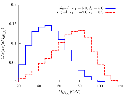
Figure 10: Normalized distribution for $M_{b\bar{b}(j)}$ for the signal process $e^{+}e^{-}\rightarrow\nu\bar{\nu}h,h\rightarrow b\bar{b}\gamma$ corresponding to the $h$-$b$-$\bar{b}$-$\gamma$ and $h$-$b$-$\bar{b}$ effective vertex scenarios at $\sqrt{s}=500$ GeV.

Accordingly, we modify I3 to demand $50~{}{\rm GeV}\leq M_{b\bar{b}(j)}\leq 110~{}{\rm GeV}$.

In Tables 8 and 9, we present our results corresponding to the signal and background processes analysed at $\sqrt{s}=$ 500 GeV and 1 TeV. The production cross-sections listed in Table 8 indicate that the rate for $e^{+}e^{-}\rightarrow\nu\bar{\nu}h,h\rightarrow b\bar{b}\gamma$ is small due to the suppression of BR($h\to b\bar{b}\gamma$). However, this scenario can still mimic the signal obtained in the $h$-$b$-$\bar{b}$-$\gamma$ effective vertex scenario due to the large contributions to the signal process arising from the other two channels.

Process	$\sqrt{s}=$500 GeV	$\sqrt{s}=$1 TeV
	$\sigma$ (pb)	$\sigma$ (pb)
$e^{+}e^{-}\rightarrow\nu\bar{\nu}h,h\rightarrow b\bar{b}\gamma$	$9.98\times 10^{-5}$	0.00023
$e^{+}e^{-}\rightarrow\nu\bar{\nu}h\gamma,h\rightarrow b\bar{b}$	0.0017	0.00523
$e^{+}e^{-}\rightarrow\nu\bar{\nu}h,h\rightarrow b\bar{b}$	0.058	0.14042

Table 8: cross sections for various processes contributing to signal at $\sqrt{s}=500$ GeV and 1 TeV. Here $c_{1}=-2.0$ and $c_{2}=0.5$.

As indicated in Table 9, these other signal contributions are significantly reduced due to our event selection and kinematic cuts which have been devised in a way such that the three-body decay of the $h$ is revealed in the signal events more prominently. Table 9 shows the number of signal background events surviving after each cuts at ${\mathcal{L}}=500~{}\mbox{${\rm fb}^{-1}$}$. As before, in this case also the most dominant contributions to the SM background arise from $e^{+}e^{-}\rightarrow\nu\bar{\nu}b\bar{b}\gamma$ and $e^{+}e^{-}\rightarrow\nu\bar{\nu}jj\gamma$ production channels. The cuts on $\cancel{E}$ and $M_{b\bar{b}(j)\gamma}$ particularly help to reduce the background events. The Higgs-driven events in Table 9 come overwhelmingly (96-97$\%$) from SM contributions, thus demonstrating that the $\{c_{1},c_{2}\}$ couplings are unlikely to make a serious difference.

	$\sqrt{s}=$500 GeV					$\sqrt{s}=$1 TeV
Process	$\sigma$ (pb)	NEV ($\mathcal{L}=$500 ${\rm fb}^{-1}$)				$\sigma$ (pb)	NEV ($\mathcal{L}=$500 ${\rm fb}^{-1}$)
		I0	I1	I2	I3		I0	I1	I2	I3
$e^{+}e^{-}\rightarrow\nu\bar{\nu}h$	$9.98\times 10^{-5}$	9	8	7	6	0.00023	21	16	14	12
$h\rightarrow b\bar{b}\gamma$
$e^{+}e^{-}\rightarrow\nu\bar{\nu}h\gamma$	0.0017	297	120	17	16	0.00523	1003	362	40	37
$h\rightarrow b\bar{b}$
$e^{+}e^{-}\rightarrow\nu\bar{\nu}h$	0.058	8	7	6	5	0.14042	20	17	15	14
$h\rightarrow b\bar{b}$
$e^{+}e^{-}\rightarrow\nu\bar{\nu}b\bar{b}\gamma$	0.00216	381	122	47	44	0.00494	983	329	95	91
$e^{+}e^{-}\rightarrow\nu\bar{\nu}b\bar{b}$	0.058	4	3	-	-	0.10880	7	6	1	1
$e^{+}e^{-}\rightarrow\nu\bar{\nu}jj\gamma$	0.0084	169	48	15	14	0.01851	398	124	34	32
$e^{+}e^{-}\rightarrow\nu\bar{\nu}jj$	0.21376	7	4	-	-	0.39883	11	8	2	2

Table 9: Cross-section and expected number of events at 500 ${\rm fb}^{-1}$ luminosity for the signal and various processes contributing to background at $\sqrt{s}=500$ GeV and 1 TeV. The Higgs-driven events include both the SM contributions and those due to non-vanishing $\{c_{1},c_{2}\}$ .

Since there are multiple channels contributing to signal process, it would be nice if one could differentiate among the various contributions by means of some kinematic variables or distributions. For this purpose we propose an observable $\Delta\phi(\gamma,\vec{\cancel{E}})$ which can be distinctly different for the process where the $\gamma$ is generated from $h$ decay or produced otherwise. We show the distribution of $\Delta\phi(\gamma,\vec{\cancel{E}})$ for the two most dominant production channels for comparison in Fig. 11.

The figure clearly shows the difference in the kinematic distribution between the two most dominant signal processes. For the process $e^{+}e^{-}\rightarrow\nu\bar{\nu}h,h\rightarrow b\bar{b}\gamma$, there is a sharp peak at larger $\Delta\phi$ as expected since the $\gamma$ is always generated from the $h$ decay. This feature can be used further in order to distinguish between the events arising from a two-body or a three-body decay of the Higgs.

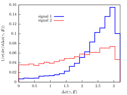
Figure 11: Normalized distribution for $\Delta\phi(\gamma,\vec{\cancel{E}})$ for the signal processes ($c_{1}=-2.0$, $c_{2}=0.5$). “signal1" and “signal2" correspond to $e^{+}e^{-}\rightarrow\nu\bar{\nu}h,h\rightarrow b\bar{b}\gamma$ and $e^{+}e^{-}\rightarrow\nu\bar{\nu}h\gamma,h\rightarrow b\bar{b}$ respectively. The plot has been done with events generated at $\sqrt{s}=500$ GeV.

Thus our study indicates that only the $h$-$b$-$\bar{b}$-$\gamma$ coupling can be probed at a relatively smaller integrated luminosity at an $e^{+}e^{-}$ collider. So far, in this section, we have discussed the discovery potential of such a scenario for $d_{1}=d_{2}=5.0$ in two possible final states, $\ell\bar{\ell}b\bar{b}\gamma$ and $b\bar{b}\gamma+\cancel{E}$ corresponding to two different centre-of-mass energies, $\sqrt{s}=250$ GeV and 500 GeV. Out of these, the latter final state at $\sqrt{s}=500$ GeV turns out to be most advantageous. Therefore, in Table 10, we have shown the required integrated luminosities in order to attain 3$\sigma$ statistical significance for different values of $d_{1}$ and $d_{2}$ for the $b\bar{b}\gamma+\cancel{E}$ final state at $\sqrt{s}=500$ GeV.

Process	Required Luminosity ($\rm fb^{-1}$)
	at $\sqrt{s}=$500 GeV
	(Final State: $b\bar{b}\gamma+\cancel{E}$)
$d_{1}=d_{2}=5.0$	6.79
$d_{1}=d_{2}=1.5$	337.5
$d_{1}=d_{2}=1.0$	1572.6

Table 10: Required integrated luminosities to attain 3$\sigma$ statistical significance corresponding to the final state $b\bar{b}\gamma+\cancel{E}$ at the centre-of-mass energy, $\sqrt{s}=500$ GeV for different values of $h$-$b$-$\bar{b}$-$\gamma$ anomalous couplings, $\{d_{1},d_{2}\}$.

IV Summary and Conclusion

We have studied the collider aspects of possible anomalous couplings of the 125 GeV Higgs with a $b\bar{b}$ pair and a photon. Such couplings have been obtained from gauge invariant effective interaction terms of dimension six. The new effective coupling parameters have been constrained from the existing Higgs measurement data at the LHC. In order to study the collider aspects of these new couplings we have concentrated on the three-body decay of the Higgs boson, $h\to b\bar{b}\gamma$. We have carried our analyses for the two different cases in the context of both LHC and a future $e^{+}e^{-}$ collider.

The $h$-$b$-$\bar{b}$-$\gamma$ effective coupling can be probed at the LHC with an integrated luminosity of the order of $2000~{}{\rm fb}^{-1}$ with $\sqrt{s}=14$ TeV. At an $e^{+}e^{-}$ collider, on the other hand, such couplings can be probed at a low luminosity at $\sqrt{s}=500$ GeV. Both results, as presented in the text, have been derived assuming $BR(h\to b\bar{b}\gamma)=5\%$ for $d_{1}=d_{2}=5.0$, which is allowed from the existing constraints on such non-standard couplings. With anomalous $h$-$b$-$\bar{b}$-$\gamma$ interaction strengths consistent with the present constraints, integrated luminosities of the order of 7 ${\rm fb}^{-1}$ are sufficient to attain $3\sigma$ statistical significance. On the other hand, even smaller values of $d_{1}$ and $d_{2}$ can be probed at an $e^{+}e^{-}$ collider. However, with the same centre-of-mass energy, in order to probe $d_{1}$, $d_{2}$ with values below 1, one has to go beyond $1000~{}{\rm fb}^{-1}$ of integrated luminosity. In contrast, $h$-$b$-$\bar{b}$ anomalous couplings are much more constrained from the Higgs measurement data and thus events driven by them give rise to smaller signal excess.

The radiative decay $h\rightarrow b\bar{b}\gamma$ with potential contributions from anomalous $h$-$b$-$\bar{b}$ interactions also contributes to similar final states and hence has been studied separately. Our analysis reveals that the expected event rates from three-body Higgs decay driven by $h$-$b$-$\bar{b}$ anomalous couplings, are unlikely to be statistically significant. We have checked that the possible enhancement in the signal rates over the SM predictions because of the presence of the non-standard couplings $\{c_{1},c_{2}\}$, consistent with their existing constraints, can be at most by a factor of 1.12. In such cases the final state arising from the three-body decay of the Higgs boson can also be mimicked by its two-body decay if a photon generated via hard scattering (not involving Higgs decay) is tagged after the cuts. Hence we have proposed a kinematic variable ($\Delta\phi(\gamma,\vec{\cancel{E}})$) that can be used to differentiate between these final state events.

V Acknowledgements

We thank N. Chakrabarty, B. Mellado, S. K. Rai, P. Saha and R. K. Singh for helpful discussions. This work is partially supported by funding available from the Department of Atomic Energy, Government of India, for the Regional Center for Accelerator- based Particle Physics (RECAPP), Harish-Chandra Research Institute. Computational work for this study was carried out at the cluster computing facility in the Harish-Chandra Research Institute (http://www.hri.res.in/cluster).

References

- Aad et al. (2012) G. Aad et al. (ATLAS), Phys. Lett. B716, 1 (2012), arXiv:1207.7214 [hep-ex] .
- Chatrchyan et al. (2012) S. Chatrchyan et al. (CMS), Phys. Lett. B716, 30 (2012), arXiv:1207.7235 [hep-ex] .
- Buchmuller and Wyler (1986) W. Buchmuller and D. Wyler, Nucl. Phys. B268, 621 (1986).
- Grzadkowski et al. (2010) B. Grzadkowski, M. Iskrzynski, M. Misiak, and J. Rosiek, JHEP 10, 085 (2010), arXiv:1008.4884 [hep-ph] .
- Dedes et al. (2017) A. Dedes, W. Materkowska, M. Paraskevas, J. Rosiek, and K. Suxho, (2017), arXiv:1704.03888 [hep-ph] .
- Aad et al. (2014) G. Aad et al. (ATLAS), Phys. Rev. D90, 112015 (2014), arXiv:1408.7084 [hep-ex] .
- Khachatryan et al. (2014) V. Khachatryan et al. (CMS), Eur. Phys. J. C74, 3076 (2014), arXiv:1407.0558 [hep-ex] .
- Aad et al. (2015a) G. Aad et al. (ATLAS), Phys. Rev. D91, 012006 (2015a), arXiv:1408.5191 [hep-ex] .
- Chatrchyan et al. (2014a) S. Chatrchyan et al. (CMS), Phys. Rev. D89, 092007 (2014a), arXiv:1312.5353 [hep-ex] .
- Aad et al. (2015b) G. Aad et al. (ATLAS), Phys. Rev. D92, 012006 (2015b), arXiv:1412.2641 [hep-ex] .
- Aad et al. (2015c) G. Aad et al. (ATLAS), JHEP 08, 137 (2015c), arXiv:1506.06641 [hep-ex] .
- Chatrchyan et al. (2014b) S. Chatrchyan et al. (CMS), JHEP 01, 096 (2014b), arXiv:1312.1129 [hep-ex] .
- Aad et al. (2015d) G. Aad et al. (ATLAS), JHEP 01, 069 (2015d), arXiv:1409.6212 [hep-ex] .
- Chatrchyan et al. (2014c) S. Chatrchyan et al. (CMS), Phys. Rev. D89, 012003 (2014c), arXiv:1310.3687 [hep-ex] .
- Aad et al. (2015e) G. Aad et al. (ATLAS), JHEP 04, 117 (2015e), arXiv:1501.04943 [hep-ex] .
- Chatrchyan et al. (2014d) S. Chatrchyan et al. (CMS), JHEP 05, 104 (2014d), arXiv:1401.5041 [hep-ex] .
- CMS (2015) ATLAS-CONF-2015-044, Tech. Rep. (2015).
- Christensen and Duhr (2009) N. D. Christensen and C. Duhr, Comput. Phys. Commun. 180, 1614 (2009), arXiv:0806.4194 [hep-ph] .
- Alloul et al. (2014) A. Alloul, N. D. Christensen, C. Degrande, C. Duhr, and B. Fuks, Comput. Phys. Commun. 185, 2250 (2014), arXiv:1310.1921 [hep-ph] .
- Aad et al. (2015f) G. Aad et al. (ATLAS), JHEP 11, 206 (2015f), arXiv:1509.00672 [hep-ex] .
- Pospelov and Ritz (2005) M. Pospelov and A. Ritz, Annals Phys. 318, 119 (2005), arXiv:hep-ph/0504231 [hep-ph] .
- Baker et al. (2006) C. A. Baker et al., Phys. Rev. Lett. 97, 131801 (2006), arXiv:hep-ex/0602020 [hep-ex] .
- Czarnecki and Krause (1997) A. Czarnecki and B. Krause, Phys. Rev. Lett. 78, 4339 (1997), arXiv:hep-ph/9704355 [hep-ph] .
- Brod et al. (2013) J. Brod, U. Haisch, and J. Zupan, JHEP 11, 180 (2013), arXiv:1310.1385 [hep-ph] .
- Gonzalez-Garcia (1999) M. C. Gonzalez-Garcia, Int. J. Mod. Phys. A14, 3121 (1999), arXiv:hep-ph/9902321 [hep-ph] .
- Han and Jiang (2001) T. Han and J. Jiang, Phys. Rev. D63, 096007 (2001), arXiv:hep-ph/0011271 [hep-ph] .
- Choi et al. (2003) S. Y. Choi, D. J. Miller, M. M. Muhlleitner, and P. M. Zerwas, Phys. Lett. B553, 61 (2003), arXiv:hep-ph/0210077 [hep-ph] .
- Han and Mellado (2010) T. Han and B. Mellado, Phys. Rev. D82, 016009 (2010), arXiv:0909.2460 [hep-ph] .
- Gao et al. (2010) Y. Gao, A. V. Gritsan, Z. Guo, K. Melnikov, M. Schulze, and N. V. Tran, Phys. Rev. D81, 075022 (2010), arXiv:1001.3396 [hep-ph] .
- De Rujula et al. (2010) A. De Rujula, J. Lykken, M. Pierini, C. Rogan, and M. Spiropulu, Phys. Rev. D82, 013003 (2010), arXiv:1001.5300 [hep-ph] .
- Desai et al. (2011) N. Desai, D. K. Ghosh, and B. Mukhopadhyaya, Phys. Rev. D83, 113004 (2011), arXiv:1104.3327 [hep-ph] .
- Boughezal et al. (2012) R. Boughezal, T. J. LeCompte, and F. Petriello, (2012), arXiv:1208.4311 [hep-ph] .
- Stolarski and Vega-Morales (2012) D. Stolarski and R. Vega-Morales, Phys. Rev. D86, 117504 (2012), arXiv:1208.4840 [hep-ph] .
- Djouadi et al. (2013) A. Djouadi, R. M. Godbole, B. Mellado, and K. Mohan, Phys. Lett. B723, 307 (2013), arXiv:1301.4965 [hep-ph] .
- Godbole et al. (2014) R. Godbole, D. J. Miller, K. Mohan, and C. D. White, Phys. Lett. B730, 275 (2014), arXiv:1306.2573 [hep-ph] .
- Banerjee et al. (2012) S. Banerjee, S. Mukhopadhyay, and B. Mukhopadhyaya, JHEP 10, 062 (2012), arXiv:1207.3588 [hep-ph] .
- Banerjee et al. (2014) S. Banerjee, S. Mukhopadhyay, and B. Mukhopadhyaya, Phys. Rev. D89, 053010 (2014), arXiv:1308.4860 [hep-ph] .
- Gunion and He (1996) J. F. Gunion and X.-G. He, Phys. Rev. Lett. 76, 4468 (1996).
- Chen et al. (2014) Y. Chen, A. Falkowski, I. Low, and R. Vega-Morales, Phys. Rev. D90, 113006 (2014), arXiv:1405.6723 [hep-ph] .
- Han et al. (2015) T. Han, Z. Liu, Z. Qian, and J. Sayre, Phys. Rev. D91, 113007 (2015), arXiv:1504.01399 [hep-ph] .
- Boudjema et al. (2015) F. Boudjema, R. M. Godbole, D. Guadagnoli, and K. A. Mohan, Phys. Rev. D92, 015019 (2015), arXiv:1501.03157 [hep-ph] .
- Braguta et al. (2003a) V. Braguta, A. Chalov, A. Likhoded, and R. Rosenfeld, Phys. Rev. Lett. 90, 241801 (2003a).
- Hagiwara et al. (2016) K. Hagiwara, K. Ma, and H. Yokoya, JHEP 06, 048 (2016), arXiv:1602.00684 [hep-ph] .
- Dwivedi et al. (2016) S. Dwivedi, D. K. Ghosh, B. Mukhopadhyaya, and A. Shivaji, Phys. Rev. D93, 115039 (2016), arXiv:1603.06195 [hep-ph] .
- Aad et al. (2016) G. Aad et al. (ATLAS), Phys. Lett. B753, 69 (2016), arXiv:1508.02507 [hep-ex] .
- Khachatryan et al. (2016) V. Khachatryan et al. (CMS), Phys. Lett. B759, 672 (2016), arXiv:1602.04305 [hep-ex] .
- Alwall et al. (2011) J. Alwall, M. Herquet, F. Maltoni, O. Mattelaer, and T. Stelzer, JHEP 06, 128 (2011), arXiv:1106.0522 [hep-ph] .
- Alwall et al. (2014) J. Alwall, R. Frederix, S. Frixione, V. Hirschi, F. Maltoni, O. Mattelaer, H. S. Shao, T. Stelzer, P. Torrielli, and M. Zaro, JHEP 07, 079 (2014), arXiv:1405.0301 [hep-ph] .
- Sjostrand et al. (2006) T. Sjostrand, S. Mrenna, and P. Z. Skands, JHEP 05, 026 (2006), arXiv:hep-ph/0603175 [hep-ph] .
- Ball et al. (2015) R. D. Ball et al. (NNPDF), JHEP 04, 040 (2015), arXiv:1410.8849 [hep-ph] .
- (51) http://cp3.irmp.ucl.ac.be/projects/madgraph/wiki/FAQ-General-13, .
- de Favereau et al. (2014) J. de Favereau, C. Delaere, P. Demin, A. Giammanco, V. Lemaître, A. Mertens, and M. Selvaggi (DELPHES 3), JHEP 02, 057 (2014), arXiv:1307.6346 [hep-ex] .
- ATL (2015) ATL-PHYS-PUB-2015-022, Tech. Rep. (2015).
- Chatrchyan et al. (2013) S. Chatrchyan et al. (CMS), JINST 8, P04013 (2013), arXiv:1211.4462 [hep-ex] .
- Cacciari et al. (2008) M. Cacciari, G. P. Salam, and G. Soyez, JHEP 04, 063 (2008), arXiv:0802.1189 [hep-ph] .
- Abramowicz et al. (2013) H. Abramowicz et al., (2013), arXiv:1306.6329 [physics.ins-det] .
- Plehn et al. (2002) T. Plehn, D. L. Rainwater, and D. Zeppenfeld, Phys. Rev. Lett. 88, 051801 (2002), arXiv:hep-ph/0105325 [hep-ph] .
- Hankele et al. (2006) V. Hankele, G. Klamke, D. Zeppenfeld, and T. Figy, Phys. Rev. D74, 095001 (2006), arXiv:hep-ph/0609075 [hep-ph] .
- (59) https://twiki.cern.ch/twiki/bin/view/LHCPhysics/HiggsEuropeanStrategy, .
- Arbey et al. (2015) A. Arbey et al., Eur. Phys. J. C75, 371 (2015), arXiv:1504.01726 [hep-ph] .
- Braguta et al. (2003b) V. Braguta, A. Chalov, A. Likhoded, and R. Rosenfeld, Phys. Rev. Lett. 90, 241801 (2003b), arXiv:hep-ph/0208133 [hep-ph] .